Pareto Frontiers in Neural Feature Learning:
Data, Compute, Width, and Luck

Abstract

In modern deep learning, algorithmic choices (such as width, depth, and learning rate) are known to modulate nuanced resource tradeoffs. This work investigates how these complexities necessarily arise for feature learning in the presence of computational-statistical gaps. We begin by considering offline sparse parity learning, a supervised classification problem which admits a statistical query lower bound for gradient-based training of a multilayer perceptron. This lower bound can be interpreted as a multi-resource tradeoff frontier: successful learning can only occur if one is sufficiently rich (large model), knowledgeable (large dataset), patient (many training iterations), or lucky (many random guesses). We show, theoretically and experimentally, that sparse initialization and increasing network width yield significant improvements in sample efficiency in this setting. Here, width plays the role of parallel search: it amplifies the probability of finding “lottery ticket” neurons, which learn sparse features more sample-efficiently. Finally, we show that the synthetic sparse parity task can be useful as a proxy for real problems requiring axis-aligned feature learning. We demonstrate improved sample efficiency on tabular classification benchmarks by using wide, sparsely-initialized MLP models; these networks sometimes outperform tuned random forests.

1 Introduction

Algorithm design in deep learning can appear to be more like “hacking” than an engineering practice. Numerous architectural choices and training heuristics can affect various performance criteria and resource costs in unpredictable ways. Moreover, it is understood that these multifarious hyperparameters all interact with each other; as a result, the task of finding the “best” deep learning algorithm for a particular scenario is foremost empirically-driven. When this delicate balance of considerations is achieved (i.e. when deep learning works well), learning is enabled by phenomena which cannot be explained by statistics or optimization in isolation. It is natural to ask: is this heterogeneity of methods and mechanisms necessary?

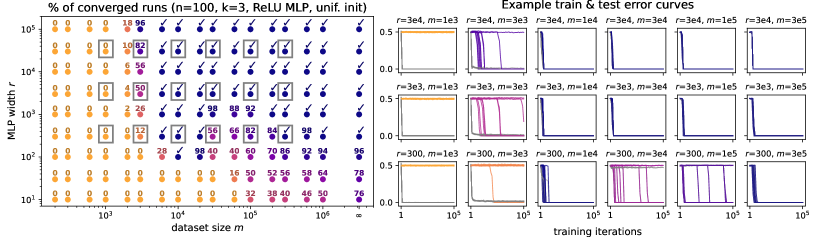
Figure 1: “More data or larger network?” Effects of jointly scaling the dataset and model sizes, for $2$-layer MLPs trained to learn sparse parities. Left: A success frontier, where the computational challenge of feature learning can be surmounted by increasing sample size or model size. Each point shows the percentage of successful training runs (out of 50 trials) for each (dataset size $m$, width $r$); $(\checkmark)$ denotes 100% successful trials. Right: 10 example training curves (gray = training error; colored = test error) for each of the boxed $(m,r)$ pairs. See main text and Section 4 for further details.

This work studies a single synthetic binary classification task in which the above complications are recognizable, and, in fact, provable. This is the problem of offline (i.e. small-sample) sparse parity learning: identify a $k$-way multiplicative interaction between $n$ Boolean variables, given $m$ random examples. We begin by interpreting the standard statistical query lower bound for this problem as a multi-resource tradeoff frontier for deep learning, balancing between the heterogeneous resources of dataset size, network size, number of iterations, and success probability. We show that in different regimes of simultaneous resource constraints (data, parallel computation, sequential computation, and random trials), the standard algorithmic choices in deep learning can succeed by diverse and entangled mechanisms. Specifically, our contributions are as follows:

Multi-resource lower and upper bounds.

We formulate a “data $\times$ width $\times$ time $\times$ luck” lower bound for offline sparse parity learning with feedforward neural nets (Theorem 3). This barrier arises from the classic statistical query (SQ) lower bound for this problem. We show that under different resource constraints, the tractability of learning can be “bought” with varied mixtures of these resources. In particular, in Theorems 4 and 5 we prove that by tuning the width and initialization scheme, we can populate this frontier with a spectrum of successful models ranging from narrow networks requiring many training samples to sample-efficient networks requiring many neurons, as summarized by the following informal theorem statement:

Informal Theorem 1.

Consider the problem of learning $(n,k)$-parities from $m$ i.i.d. samples with a $2$-layer width-$r$ ReLU MLP, whose first-layer neurons are initialized with sparsity $s$. After $O_{n}(1)$ steps of gradient descent, the $k$ relevant coordinates are identified with probability 0.99 when (1) $s>\Omega(k)$, $r=\Theta((n/s)^{k})$ and $m=\Theta(n^{2}(s/k)^{k-1})$, and when (2) $s<k$, $r=\Theta((n/k)^{s})$ and $m=\Theta((n/k)^{k-s-1})$.

Intuitively, this analysis reveals a feature learning mechanism by which overparameterization (i.e. large network width) plays a role of parallel search over randomized subnetworks. Each individual hidden-layer neuron has its own sample complexity for identifying the relevant coordinates, based on its Fourier gap (Barak et al.,, 2022) at initialization. Trained with parallel gradient updates, the full network implicitly acts as an ensemble model over these neurons, whose overall sample complexity is determined by the “winning lottery tickets” (Frankle and Carbin,, 2018) (i.e. the lucky neurons initialized to have the lowest sample complexity). This departs significantly from the neural tangent kernel (Jacot et al.,, 2018) regime of function approximation with wide networks, in which overparameterization removes data-dependent feature selection (rather than parallelizing it across subnetworks).

Empirical study of neural nets’ statistical thresholds for sparse parity learning.

We corroborate the theoretical analysis with a systematic empirical study of offline sparse parity learning using SGD on MLPs, demonstrating some of the (perhaps) counterintuitive effects of width, data, and initialization. For example, Figure 1 highlights our empirical investigation into the interactions between data, width, and success probability. The left figure shows the fractions of successful training runs as a function of dataset size (x-axis) and width (y-axis). Roughly, we see a “success frontier”, where having a larger width can be traded off with smaller sample sizes. The right figure depicts some training curves (for various widths and sample sizes). Grokking (Power et al.,, 2022; Liu et al.,, 2022) (discontinuous and delayed generalization behavior induced by optimization dynamics) is evident in some of these figures.

“Parity2real” transfer of algorithmic improvements.

It is often observed that deep learning methods underperform tree-based methods (e.g. random forests) on tabular datasets, particularly those where the target function depends on a few of the input features in a potentially non-smooth manner; see Grinsztajn et al., (2022) for a recent discussion. Motivated by our findings in the synthetic parity setting (and the observation that the sparse parity task possesses a number of the same properties of these problematic real-world datasets), we then turn to experimentally determine the extent to which our findings also hold for real tabular data. We evaluate MLPs of various depths and initialization sparsities on 16 tabular classification tasks, which were standardized by Grinsztajn et al., (2022) to compare neural vs. tree-based methods. Figure 3 shows that wider networks and sparse initialization yield improved performance, as in the parity setting. In some cases, our MLPs outperform tuned random forests.

1.1 Related work

In the nascent empirical science of large-scale deep learning, scaling laws (Kaplan et al.,, 2020; Hoffmann et al.,, 2022) have been shown to extrapolate model performance with remarkable consistency, revealing flexible tradeoffs and Pareto frontiers between the heterogeneous resources of data and computation. The present work reveals that in the simple synthetic setting of parity learning, the same intricacies can be studied theoretically and experimentally. In particular, viewing model size $\times$ training iterations $\times$ random restarts as a single “total FLOPs” resource, our study explains why data $\times$ compute can be a necessary and sufficient resource, through the lens of SQ complexity.

Analyses of deep feature learning.

Formally characterizing the representation learning mechanisms of neural networks is a core research program of deep learning theory. Many recent works have analyzed gradient-based feature learning (Wei et al.,, 2019; Barak et al.,, 2022; Zhenmei et al.,, 2022; Abbe et al.,, 2022; Damian et al.,, 2022; Telgarsky,, 2022), escaping the “lazy” neural tangent kernel (NTK) regime (Jacot et al.,, 2018; Chizat et al.,, 2019), in which features are fixed at initialization.

Learning parities with neural networks.

The XOR function has been studied as an elementary challenging example since the dawn of artificial neural networks (Minsky and Papert,, 1969), and has been revisited at various times: e.g. neural cryptography (Rosen-Zvi et al.,, 2002); learning interactions via hints in the input distribution (Daniely and Malach,, 2020); a hard case for self-attention architectures (Hahn,, 2020). Closest to this work, Barak et al., (2022) find that in the case of online (infinite-data) parity learning, SGD provides a feature learning signal for a single neuron, and can thus converge at a near-optimal computational rate for non-overparameterized networks. They note computational-statistical tradeoffs and grokking in the offline setting, which we address systematically. Merrill et al., (2023) examine the same problem setting empirically, investigating a mechanism of competing sparse and dense sub-networks. Abbe et al., (2023) provide evidence that the time complexity required by an MLP to learn an arbitrary sparse Boolean function is governed by the largest “leap” in the staircase of its monomials, each of which is a sparse parity. Telgarsky, (2022) gives a margin-based analysis of gradient flow on a two-layer neural network that achieves improved sample complexity ($\tilde{O}(n/\epsilon)$) for the 2-sparse parity problem, at the cost of exponential width.

Neural nets and axis-aligned tabular data.

Decision tree ensembles such as random forests (Breiman,, 2001) and XGBoost (Chen and Guestrin,, 2016) remain more popular among practitioners than neural networks on tabular data (Kaggle,, 2021), despite many recent attempts to design specialized deep learning methods (Borisov et al.,, 2022). Some of these employ sparse networks (Yang et al., 2022b, ; Lutz et al.,, 2022) similar to those considered in our theory and experiments.

We refer the reader to Appendix A for additional related work.

2 Background

2.1 Parities, and parity learning algorithms

A light bulb is controlled by $k$ out of $n$ binary switches; each of the $k$ influential switches can toggle the light bulb’s state from any configuration. The task in parity learning is to identify the subset of $k$ important switches, given access to $m$ i.i.d. uniform samples of the state of all $n$ switches. Formally, for any $1\leq k\leq n$ and $S\subseteq[n]$ such that $|S|=k$, the parity function $\chi_{S}:\{\pm 1\}^{n}\rightarrow\pm 1$ is defined as $\chi_{S}(x_{1:n}):=\prod_{i\in S}x_{i}$. The $(n,k)$-parity learning problem is to identify $S$ from samples $(x\sim\mathrm{Unif}(\{\pm 1\}^{n},y=\chi_{S}(x)))$; i.e. output a classifier with $100$% accuracy on this distribution, without prior knowledge of $S$.

This problem has a rich history in theoretical computer science, information theory, and cryptography. There are several pertinent ways to think about the fundamental role of parity learning:

1. Monomial basis elements: A $k$-sparse parity is a degree-$k$ monomial, and thus the analogue of a Fourier coefficient with “frequency” $k$ in the harmonic analysis of Boolean functions (O’Donnell,, 2014). Parities form an important basis for polynomial learning algorithms (e.g. Andoni et al., (2014)).

2. Computational hardness: There is a widely conjectured computational-statistical gap for this problem (Applebaum et al.,, 2009, 2010), which has been proven in restricted models such as SQ (Kearns,, 1998) and streaming (Kol et al.,, 2017) algorithms. The statistical limit is $\Theta(\log(\text{number of possibilities for }S))=\Theta(k\log n)$ samples, but the amount of computation needed (for an algorithm that can tolerate an $O(1)$ fraction of noise) is believed to scale as $\Omega(n^{ck})$ for some constant $c>0$ – i.e., there is no significant improvement over trying all subsets.

3. Feature learning: This setting captures the learning of a concept which depends jointly on multiple attributes of the inputs, where the lower-order interactions (i.e. correlations with degree-$k^{\prime}<k$ parities) give no information about $S$. Intuitively, samples from the sparse parity distribution look like random noise until the learner has identified the sparse interaction. This notion of feature learning complexity is also captured by the more general information exponent (Ben Arous et al.,, 2021).

2.2 Notation for neural networks

For single-output regression, a 2-layer multi-layer perceptron (MLP) is a function class, parameterized by a matrix $W\in\mathbb{R}^{r\times n}$, vectors $v,b\in\mathbb{R}^{r}$ and scalar $\beta\in{\mathbb{R}}$, defined by

$$\widehat{y}:x\mapsto v^{\top}\sigma(Wx+b)+\beta,$$

where $\sigma$ is an activation function, usually a scalar function applied identically to each input. For rows $w_{i}$ of $W$, the intermediate variables $\sigma(w_{i}^{\top}x+b_{i})$ are thought of as hidden layer activations or neurons. The number of parallel neurons is often called the width.

3 Theory

In this section we theoretically study the interactions between data, width, time, and luck on the sparse parity problem. We begin by rehashing Statistical Query (SQ) lower bounds for parity learning in the context of gradient-based optimization, showing that without sufficient resources sparse parities cannot be learned. Then, we prove upper bounds showing that parity learning is possible with correctly scaling either width (keeping sample size small), sample size (keeping width small), or a mixture of the two.

Statistical query algorithms.

A seminal work by Kearns, (1998) introduced the statistical query (SQ) algorithm framework, which provides a means of analyzing noise-tolerant algorithms. Unlike traditional learning algorithms, SQ algorithms lack access to individual examples but can instead make queries to an SQ oracle, which responds with noisy estimates of the queries over the population. Notably, many common learning algorithms, including noisy variants of gradient descent, can be implemented within this framework. While SQ learning offers robust guarantees for learning in the presence of noise, there exist certain problems that are learnable from examples but not efficiently learnable from statistical queries (Blum et al.,, 1994, 2003). One notable example of such a problem is the parity learning problem, which possesses an SQ lower bound. This lower bound can be leveraged to demonstrate the computational hardness of learning parities with gradient-based algorithms (e.g., Shalev-Shwartz et al., (2017)).

3.1 Lower bound: a multi-resource hardness frontier

We show a version of the SQ lower bound in this section. Assume we optimize some model $h_{\theta}$, where $\theta\in{\mathbb{R}}^{r}$ (i.e., $r$ parameters). Let $\ell$ be some loss function satisfying: $\ell^{\prime}(\hat{y},y)=-y+\ell_{0}(\hat{y})$; for example, one can choose $\ell_{2}(\hat{y},y)=\frac{1}{2}(y-\hat{y})^{2}$. Fix some hypothesis $h$, target $f$, a sample ${\cal S}\subseteq\{\pm 1\}^{n}$ and distribution ${\cal D}$ over $\{\pm 1\}^{n}$. We denote the empirical loss by $L_{\cal S}(h,f)=\frac{1}{\left\lvert{\cal S}\right\rvert}\sum_{{\mathbf{x}}\in{\cal S}}\ell(h({\mathbf{x}}),f({\mathbf{x}}))$ and the population loss by $L_{\cal D}(h,f):=\operatorname*{\mathbb{E}}_{{\mathbf{x}}\sim{\cal D}}\left[\ell(h({\mathbf{x}}),f({\mathbf{x}}))\right]$. We consider SGD updates of the form:

$$\theta_{t+1}=\theta_{t}-\eta_{t}\left(\nabla_{\theta}\left(L_{{\cal S}_{t}}(h_{\theta_{t}},f)+R(\theta_{t})\right)+\xi_{t}\right),$$

for some sample ${\cal S}_{t}$, step size $\eta_{t}$, regularizer $R(\cdot)$, and adversarial noise $\xi_{t}\in[-\tau,\tau]^{r}$. For normalization, we assume that $\left\lVert\nabla h_{\theta}({\mathbf{x}})\right\rVert_{\infty}\leq 1$ for all $\theta$ and ${\mathbf{x}}\in{\cal X}$.

Denote by $\mathbf{0}$ the constant function, mapping all inputs to $0$. Let $\theta^{\star}_{t}$ be the following trajectory of SGD that is independent of the target. Define $\theta^{\star}_{t}$ recursively s.t. $\theta^{\star}_{0}=\theta_{0}$ and

$$\theta^{\star}_{t+1}=\theta^{\star}_{t}-\eta_{t}\nabla_{\theta}\left(L_{\cal D}(h_{\theta^{\star}_{t}},\mathbf{0})+R(\theta^{\star}_{t})\right)$$

Assumption 2 (Bounded error for gradient estimator).

For all $t$, suppose that

$$\left\lVert\nabla L_{{\cal S}_{t}}(h_{\theta^{\star}_{t}},\mathbf{0})-\nabla L_{{\cal D}}(h_{\theta^{\star}_{t}},\mathbf{0})\right\rVert_{\infty}\leq\tau/2.$$

Remark: If $m=\tilde{O}(1/\tau^{2})$, Assumption 2 is satisfied w.h.p. for: 1) ${\cal S}_{t}\sim{\cal D}^{m}$ (“online” SGD), 2) ${\cal S}_{t}={\cal S}$ for some ${\cal S}\sim{\cal D}^{m}$ (“offline” GD) and 3) ${\cal S}_{t}$ is a batch of size $m$ sampled uniformly at random from ${\cal S}$, where ${\cal S}\sim{\cal D}^{M}$ and $M\geq m$ (“offline” SGD). Indeed, in all these cases we have $\operatorname*{\mathbb{E}}_{{\cal S}_{t}}\left[\nabla L_{{\cal S}_{t}}(h_{\theta^{\star}_{t}},\mathbf{0})\right]=\nabla L_{\cal D}(h_{\theta^{\star}_{t}},\mathbf{0})$, and the above follows from standard concentration bounds.

The lower bound in this section uses standard statistical query arguments to show that gradient-based algorithms, without sufficient resources, will fail to learn $(n,k)$-parities. We therefore start by stating the four types of resources that impact learnability:

• The number of parameters $r$ – equivalently, the number of parallel “queries”.

• The number of gradient updates $T$ – i.e. the serial running time of the training algorithm.

• The gradient precision $\tau$ – i.e. how close the empirical gradient is to the population gradient. As discussed above, $\tilde{O}(1/\tau^{2})$ samples suffice to obtain such an estimator.

• The probability of success $\delta$.

The following theorem ties these four resources together, showing that without a sufficient allocation of these resources, gradient descent will fail to learn:

Proposition 3.

Assume that $\theta_{0}$ is randomly drawn from some distribution. For every $r,T,\delta,\tau>0$, if $\frac{rT}{\tau^{2}\delta}\leq\frac{1}{2}\binom{n}{k}$, then there exists some $(n,k)$-parity s.t. with probability at least $1-\delta$ over the choice of $\theta_{0}$, the first $T$ iterates of SGD are statistically independent of the target function.

The proof follows standard SQ lower bound arguments (Kearns,, 1998; Feldman,, 2008), and for completeness is given in Appendix B. The core idea of the proof is the observation that any gradient step has very little correlation (roughly $n^{-k}$) with most sparse-parity functions, and so there exists a parity function that has small correlation with all steps. In this case, the noise can force the gradient iterates to follow the trajectory $\theta^{\star}_{1},\dots,\theta^{\star}_{T}$, which is independent of the true target. We note that, while the focus of this paper is on sparse parities, similar analysis applies for a broader class of functions that are characterized by large SQ dimension (see Blum et al., (1994)).

Observe that there are various ways for an algorithm to escape the lower bound of Theorem 3. We can scale a single resource with $\binom{n}{k}$, keeping the rest small, e.g. by training a network of size $n^{k}$, or using a sample size of size $n^{k}$. Crucially, we note the possibility of interpolating between these extremes: one can spread this homogenized “cost” across multiple resources, by (e.g.) training a network of size $n^{k/2}$ using $n^{k/2}$ samples. In the next section, we show how neural networks can be tailored to solve the task in these interpolated resource scaling regimes.

3.2 Upper bounds: many ways to trade off the terms

As a warmup, we discuss some simple SQ algorithms that succeed in learning parities by properly scaling the different resources. First, consider deterministic exhaustive search, which computes the error of all possible $(n,k)$-parities, choosing the one with smallest error. This can be done with constant $\tau$ (thus, sample complexity logarithmic in $n$), but takes $T=\Theta(n^{k})$ time. Since querying different parities can be done in parallel, we can reduce the number of steps $T$ by increasing the number of parallel queries $r$. Alternatively, it is possible to query only a randomly selected subset of parities, which reduces the overall number of queries but increases the probability of failure.

The above algorithms give a rough understanding of the frontier of algorithms that succeed at learning parities. However, at first glance, they do not seem to reflect algorithms used in deep learning, and are specialized to the parity problem. In this section, we will explore the ability of neural networks to achieve similar tradeoffs between the different resources. In particular, we focus on the interaction between sample complexity and network size, establishing learning guarantees with interpolatable mixtures of these resources.

Before introducing our main positive theoretical results, we discuss some prior theoretical results on learning with neural networks, and their limitations in the context of learning parities. Positive results on learning with neural networks can generally be classified into two categories: those that reduce the problem to convex learning of linear predictors over a predefined set of features (e.g. the NTK), and those that involve neural networks departing from the kernel regime by modifying the fixed features of the initialization, known as the feature learning regime.

Kernel regime.

When neural networks trained with gradient descent stay close to their initial weights, optimization behaves like kernel regression on the neural tangent kernel (Jacot et al.,, 2018; Du et al.,, 2018): the resulting function is approximately of the form ${\mathbf{x}}\mapsto\left\langle\psi({\mathbf{x}}),{\mathbf{w}}\right\rangle$, where $\psi$ is a data-independent infinite-dimensional embedding of the input, and ${\mathbf{w}}$ is some weighting of the features. However, it has been shown that the NTK (more generally, any fixed kernel) cannot achieve low $\ell_{2}$ error on the $(n,k)$-parity problem, unless the sample complexity grows as $\Omega(n^{k})$ (see Kamath et al., (2020)). Thus, no matter how we scale the network size or training time, neural networks trained in the NTK regime cannot learn parities with low sample complexity, and thus do not enjoy the flexibility of resource allocation discussed above.

Feature learning regime.

Due to the limitation of neural networks trained in the kernel regime, some works study learning in the “rich” regime, quantifying how hidden-layer features adapt to the data. Among these, Barak et al., (2022) analyze a feature learning mechanism requiring exceptionally small network width: SGD on 2-layer MLPs can solve the online sparse parity learning problem with network width independent of $n$ (dependent only on $k$), at the expense of requiring a suboptimal ($\approx n^{k}$) number of examples. This mechanism is Fourier gap amplification, by which SGD through a single neuron $\sigma(w^{\top}x)$ can perform feature selection in this setting, via exploiting a small gap between the relevant and irrelevant coordinates in the population gradient. The proof of Theorem 4 below relies on a similar analysis, extended to the offline regime (i.e., multiple passes over a dataset of limited size).

3.2.1 “Data $\!\times\!$ model size” success frontier for sparsely-initialized MLPs

In this section, we analyze a 2-layer MLP with ReLU ($\sigma(x)=\max(0,x)$) activation, trained with batch (“offline”) gradient-descent over a sample ${\cal S}$ with $\ell_{2}$-regularized updates:

$$\theta^{(t+1)}=(1-\lambda^{(t)})\theta^{(t)}-\eta^{(t)}\nabla L_{\cal S}(h_{\theta^{(t)}})$$

We allow learning rates $\eta$, and weight decay coefficients $\lambda$ to differ between layers and iterations. For simplicity, we analyze the case where no additional noise is added to each update; however, we believe that similar results can be obtained in the noisy case (e.g., using the techniques in Feldman et al., (2017)). Finally, we focus on ReLU networks with $s$-sparse initialization of the first layer: every weight ${\mathbf{w}}_{i}$ has $s$ randomly chosen coordinates set to $1$, and the rest set to $0$. Note that after initialization, all of the network’s weights are allowed to move, so sparsity is not necessarily preserved during training.

Over-sparse initialization ($s>\Omega(k)$).

The following theorem demonstrates a “data $\!\times\!$ width” success frontier when learning $(n,k)$-parities with sparsely initialized ReLU MLPs at sparsity levels $s>\Omega(k)$.

Theorem 4.

Let $k$ be an even integer, and $\epsilon\in(0,1/2)$. Assume that $n\geq\Omega(1/\epsilon^{2})$. For constants $c_{1},c_{2},c_{3},c_{4}$ depending only on $k$, choose the following: (1) sparsity level: $s\geq c_{1}/\epsilon^{2}$, for some odd $s$, (2) width of the network: $r=c_{2}(n/s)^{k}$, (3) sample size: $m\geq c_{3}(s/k)^{k-1}n^{2}\log n$, and (4) number of iterations: $T\geq c_{4}/\epsilon^{2}$. Then, for every $(n,k)$-parity distribution ${\cal D}$, with probability at least $0.99$ over the random samples and initialization, gradient descent with these parameter settings returns a function $h_{T}$ s.t. $L_{\cal D}(h_{T})\leq\epsilon$.

Intuitively, by varying the sparsity parameter in Theorem 4, we obtain a family of algorithms which smoothly interpolate between the small-data/large-width and large-data/small-width regimes of tractability. First, consider a sparsity level linear in $n$ (i.e. $s=\alpha\cdot n$). In this case, a small network (with width $r$ independent of the input dimension) is sufficient for solving the problem, but the sample size must be large ($\Omega(n^{k+1})$) for successful learning; this recovers the result of Barak et al., (2022). At the other extreme, if the sparsity is independent of $n$, the sample complexity grows only as $O(n^{2}\log n)$, but the requisite width becomes $\Omega(n^{k})$.

Proof sketch. The proof of Theorem 4 relies on establishing a Fourier anti-concentration condition, separating the relevant (i.e. indices in $S$) and irrelevant weights in the initial population gradient, similarly as the main result in Barak et al., (2022). When we initialize an $s$-sparse neuron, there is a probability of $\gtrsim(s/n)^{k}$ that the subset of activated weights contains the “correct” subset $S$. In this case, to detect the subset $S$ via the Fourier gap, it is sufficient to observe $s^{k-1}$ examples instead of $n^{k-1}$. Initializing the neurons more sparsely makes it less probable to draw a lucky neuron, but once we draw a lucky neuron, it requires fewer samples to find the right features. Thus, increasing the width reduces overall sample complexity, by sampling a large number of “lottery tickets”.

Under-sparse initialization ($s<k$).

The sparsity parameter can modulate similar data vs. width tradeoffs for feature learning in the “under-sparse” regime. We provide a partial analysis for this more challenging case, showing that one step of gradient descent can recover a correct subnetwork. Appendix B.3 discusses the mathematical obstructions towards obtaining an end-to-end guarantee of global convergence.

Theorem 5.

For even $k,s$, sparsity level $s<k$, network width $r=O((n/k)^{s})$, and $\varepsilon$-perturbed $s$-sparse random initialization scheme s.t. for every $(n,k)$-parity distribution ${\cal D}$, with probability at least $0.99$ over the choice of sample and initialization after one step of batch gradient descent (with gradient clipping) with sample size $m=O((n/k)^{k-s-1})$ and appropriate learning rate, there is a subnetwork in the ReLU MLP that approximately computes the parity function.

Here, the sample complexity can be improved by a factor of $n^{s}$, at the cost of requiring the width to be $n^{s}$ times larger. The proof of Theorem 5 relies on a novel analysis of improved Fourier gaps with “partial progress”: intuitively, if a neuron is randomly initialized with a subset of the relevant indices $S$, it only needs to identify $k-s$ more coordinates, inheriting the improved sample complexity for the $(n-s,k-s)$-parity problem. Note that the probability of finding such a lucky neuron scales as $(n/k)^{-s}$, which governs how wide (number of lottery tickets) the network needs to be.

Remarks on the exact-sparsity regime.

Our theoretical analyses do not extend straightforwardly to the case of $s=\Theta(k)$. Observe that if the value of $k$ is known, initializing a network of size $r=\widetilde{O}\left(n^{k}\right)$ with sparsity $s=k$ gives w.h.p. a subnetwork with good first-layer features at initialization. We believe that with a proper choice of regularization and training scheme, it is possible to show that such a network learns to select this subnetwork with low sample complexity. We leave the exact details of this construction and end-to-end proofs for future work.

Analogous results for dense initialization schemes?

We believe that the principle of “parallel search with randomized per-subnetwork sample complexities” extends to other initialization schemes (including those more commonly used in practice), and leads to analogous success frontiers. To support this, our experiments investigate both sparse and uniform initialization, with qualitatively similar findings. For dense initializations, the mathematical challenge lies in analyzing the Fourier anti-concentration of general halfspaces (see the discussion and experiments in Appendix C.1 of (Barak et al.,, 2022)). The axis-aligned inductive biases imparted by sparse initialization may also be of independent practical interest.

4 Experiments

A high-level takeaway from Section 3 is that when a learning problem is computationally difficult but statistically easy, a complex frontier of resource tradeoffs can emerge; moreover, it is possible to interpolate between extremes along this frontier using ubiquitous algorithmic choices in deep learning, such as overparameterization, random initialization, and weight decay. In this section, we explore the nature of the frontier with an empirical lens—first with end-to-end sparse parity learning, then with natural tabular datasets.

4.1 Empirical Pareto frontiers for offline sparse parity learning

We launch a large-scale ($\sim$200K GPU training runs) exploration of resource tradeoffs when training neural networks to solve the offline sparse parity problem. While Section 3 analyzes idealized variants of SGD on MLPs which interpolate along the problem’s resource tradeoff frontier, in this section we ask whether the same can be observed end-to-end with standard training and regularization.

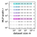
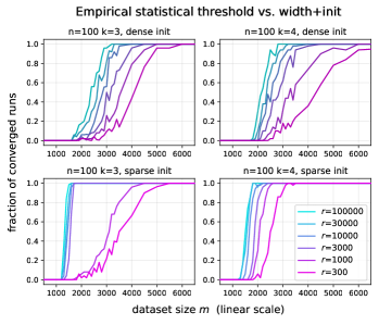
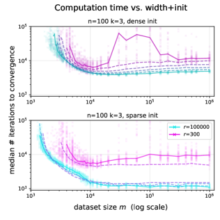
Figure 2: Zoomed-in views of the interactions between width, data, time, and luck. Left: Locations of these runs in the larger parameter space. Center: Success probability vs. dataset size. In accordance with our theory, width buys luck, and improves end-to-end sample efficiency, despite increasing the network’s capacity. Right: Number of iterations to convergence vs. dataset size. We observe a data vs. time tradeoff in the grokking regime (at the edge of feasibility), as well as a “sample-wise double descent” performance drop with more data (which can also be seen in Figure 1, and disappears with larger widths). Comparing dense vs. sparse initializations (upper vs. lower plots; sparse inits are colored more brightly), we see computational and statistical benefits of the sparse initialization scheme from Section 3.2.1.

On various instances of the $(n,k)$-sparse parity learning problem, we train a 2-layer MLP with identical hyperparameters, varying the network width $r\in\{10,30,100,\ldots,10^{5}\}$ and the dataset size $m\in\{100,200,300,600,1000,\ldots,10^{6}\}$. Alongside standard algorithmic choices, we consider one non-standard augmentation of SGD: the under-sparse initialization scheme from Section 3.2.1; we have proven that these give rise to “lottery ticket” neurons which learn the influential coordinates more sample-efficiently. Figure 1 (in the introduction) and Figure 2 illustrate our findings at a high level; details and additional discussion are in Appendix C.1). We list our key findings below:

1. A “success frontier”: large width can compensate for small datasets. We observe convergence and perfect generalization when $m\ll n^{k}$. In such regimes, which are far outside the online setting considered by Barak et al., (2022), high-probability sample-efficient learning is enabled by large width. This can be seen in Figure 1 (left), and analogous plots in Appendix C.1.

2. Width is monotonically beneficial, and buys data, time, and luck. In this setting, increasing the model size yields exclusively positive effects on success probability, sample efficiency, and the number of serial steps to convergence (see Figure 2). This is a striking example where end-to-end generalization behavior runs opposite to uniform convergence-based upper bounds, which predict that enlarging the model’s capacity worsens generalization.

3. Sparse axis-aligned initialization buys data, time, and luck. Used in conjunction with a wide network, we observe that a sparse, axis-aligned initialization scheme yields strong improvements on all of these axes; see Figure 2 (bottom row). In smaller hyperparameter sweeps, we find that $s=2$ (i.e. initialize every hidden-layer neuron with a random $2$-hot weight vector) works best.

4. Intriguing effects of dataset size. As we vary the sample size $m$, we note two interesting phenomena; see Figure 2 (right). The first is grokking (Power et al.,, 2022), which has been previously documented in this setting (Barak et al.,, 2022; Merrill et al.,, 2023). This entails a data vs. time tradeoff: for small $m$ where learning is marginally feasible, optimization requires significantly more training iterations $T$. Our second observation is a “sample-wise double descent” (Nakkiran et al.,, 2021): success probability and convergence times can worsen with increasing data. Both of these effects are also evident in Figure 1).

Lottery ticket neurons.

The above findings are consistent with the viewpoint taken by the theoretical analysis, where randomly-initialized SGD plays the role of parallel search, and a large width increases the number of random subnetworks available for this process—in particular, the “winning lottery ticket” neurons, for which feature learning occurs more sample-efficiently. To provide further evidence that sparse subnetworks are responsible for learning the parities, we perform a smaller-scale study of network prunability in Appendix C.2.

4.2 Sample-efficient deep learning on natural tabular datasets

Sparse parity learning is a toy problem, in that it is defined by an idealized distribution, averting the ambiguities inherent in reasoning about real-life datasets. However, due to its provable hardness (Theorem 3, as well as the discussion in Section 2.1), it is a maximally hard toy problem in a rigorous sense. In this section, we perform a preliminary investigation of how the empirical and algorithmic insights gleaned from Section 4.1 can be transferred to more realistic learning scenarios.

To this end, we use the benchmark assembled by Grinsztajn et al., (2022), a work which specifically investigates the performance gap between neural networks and tree-based classifiers (e.g. random forests, gradient-boosted trees), and includes a standardized suite of 16 classification benchmarks with numerical input features. The authors identify three common aspects of tabular tasks which present difficulties for neural networks, especially vanilla MLPs:

• The feature spaces are not rotationally invariant. In state-of-the-art deep learning, MLPs are often tasked with function representation in rotation-invariant domains (token embedding spaces, convolutional channels, etc.).

• Many of the features are uninformative. In order to generalize effectively, especially from a limited amount of data, it is essential to avoid overfitting to these features.

• There are meaningful high-frequency/non-smooth patterns in the target function. Combined with property (i), decision tree-based methods (which typically split on axis-aligned features) can appear to have the ideal inductive bias for tabular modalities of data.

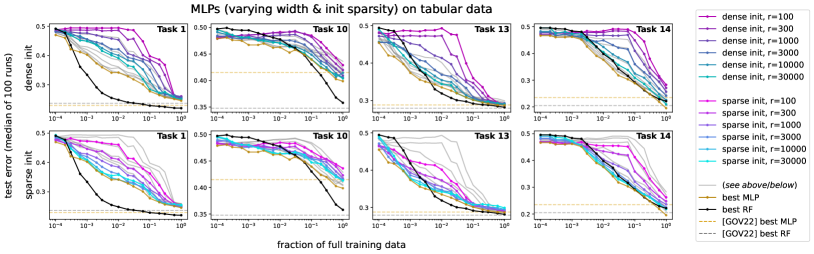
Figure 3: Analogous investigation of MLP width $r$ and sparse initialization for real-world tabular datasets (OpenML benchmarks assembled by Grinsztajn et al., (2022)), varying the dataset size $m$ via downsampling. Large width and sparse initialization tend to improve generalization, in accordance with the theory and experiments for synthetic parity tasks. In some settings, our best MLPs outperform tuned random forests. Dotted lines denote the test errors reported by Grinsztajn et al., (2022) of tuned MLPs and RFs on the full datasets. Full results on all 16 tasks are in Appendix C.3.

Noting that the sparse parity task possesses all three of the above qualities, we conduct a preliminary investigation on whether our empirical findings in the synthetic case carry over to natural tabular data. In order to study the impact of algorithmic choices (mainly width and sparse initialization) on sample efficiency, we create low-data problem instances by subsampling varying fractions of each dataset for training. Figure 3 provides a selection of our results. We note the following empirical findings, which are the tabular data counterparts of results (2) and (3) in Section 4.1:

• Wide networks generalize on small tabular datasets. Like in the synthetic experiments, width yields nearly monotonic end-to-end benefits for learning. This suggests that the “parallel search + pruning” mechanisms analyzed in our paper are also at play in these settings. In some (but not all) cases, these MLPs perform competitively with tuned tree-based classifiers.

• Sparse axis-aligned initialization sometimes improves end-to-end performance. This effect is especially pronounced on datasets which are downsampled to be orders of magnitude smaller. We believe that this class of drop-in replacements for standard initialization merits further investigation, and may contribute to closing the remaining performance gap between deep learning and tree ensembles on small tabular datasets.

5 Conclusion

We have presented a theoretical and empirical study of offline sparse parity learning with neural networks; this is a provably hard problem which admits a multi-resource lower bound in the SQ model. We have shown that the lower bound can be surmounted using varied mixtures of these resources, which correspond to natural algorithmic choices and scaling axes in deep learning. By investigating how these choices influence the empirical “success frontier” for this hard synthetic problem, we have arrived at some promising improvements for MLP models of tabular data (namely, large width and sparse initialization). These preliminary experiments suggest that a more intensive, exhaustive study of algorithmic improvements for MLPs on tabular data has a chance of reaping significant rewards, perhaps even surpassing the performance of decision tree ensembles.

Broader impacts and limitations.

The nature of this work is foundational; the aim of our theoretical and empirical investigations is to contribute to the fundamental understanding of neural feature learning, and the influences of scaling relevant resources. A key limitation is that our benchmarks on tabular data are only preliminary; it is a significant and perennial methodological challenge to devise fair and comprehensive comparisons between neural networks and tree-based learning paradigms.

Part I Appendix

Appendix A Additional related work

Learning parities with neural networks.

Parities (or XORs) have been shown to be computationally hard to learn for SQ algorithms including gradient-based methods. Various works make additional assumptions to avoid these hardness results to show that neural networks can be efficiently trained to learn parities (Daniely and Malach,, 2020; Shi et al.,, 2021; Frei et al.,, 2022; Malach et al.,, 2021). More recently, Barak et al., (2022) have focused on understanding how neural networks training on parities without any additional assumption behaves at this computational-statistical limit. They show that one step of gradient descent on a single neuron is able to recover the indices corresponding to the parity with $n^{O(k)}$ samples/computation. Abbe et al., (2023) improve this bound to $O(n^{k-1})$ online SGD steps and generalize the result to handle hierarchical staircases of parity functions which requires a multi-step analysis. Telgarsky, (2022) studies the problem of 2-sparse parities with two-layer neural networks trained with vanilla SGD (unlike our restricted two-step training algorithm) and studies the margins achieved post training. They use the margins to get optimal sample complexity $\tilde{O}(n^{2}/\epsilon)$ in the NTK regime. Going beyond NTK, they analyze gradient flow (with certain additional modifications) on an exponential wide 2-layer network (making it computationally inefficient) to get the improved sample complexity of $\tilde{O}(n/\epsilon)$. In contrast to this, our goal is to improve sample complexity while maintaining computational efficiency, using random guessing via the sparse initialization.

Learning single-index/multi-index models over Gaussians with neural networks.

Another line of work (Ben Arous et al.,, 2021; Ba et al.,, 2022; Damian et al.,, 2022; Bietti et al.,, 2022; Damian et al.,, 2023) has focused on learning functions that depend on a few directions, in particular, single-index and multi-index models over Gaussians using neural nets. These can be thought of as a continuous analog to our sparse parity problem. In a similar analysis (as parities) of online SGD for single index models, Ben Arous et al., (2021) propose the notion of an information exponent which captures the initial correlation between the model and the target function, and get convergence results similar to the parity setting with sample complexity $O(n^{k-1})$ for information exponent $k$ (can be thought similar to the $k$ in the parity learning problem). Damian et al., (2023) improve this result by showing that a smoothed version of GD achieves the optimal sample complexity (for CSQ algorithms) of $(n^{k/2})$. Going beyond CSQ algorithms, Chen and Meka, (2020) provide a filtered-PCA algorithm that achieves polynomial dependence on the dimension $n$ in both compute and sample complexity. Note that this is not achievable for CSQ algorithms. For the parity learning problem, the SQ computational lower bounds are $\Omega(n^{k})$ (as described in Section 3.1).

Empirical inductive biases of large MLPs.

Our experiments on tabular benchmarks suggest that wide and sparsely-initialized vanilla MLPs can sometimes close the performance gap between neural networks and decision tree ensemble methods. This corroborates recent findings that vanilla MLPs have strong enough inductive biases to generalize nontrivially in natural data modalities, despite the overparameterization and lack of architectural biases via convolution or recurrence. Notably, many state-of-the-art computer vision models have removed convolutions (Dosovitskiy et al.,, 2020; Tolstikhin et al.,, 2021); recently, (Bachmann et al.,, 2023) demonstrate that even large vanilla NLPs can compete with convolutional models for image classification. Yang et al., 2022a find monotonic improvements in terms of model width, which are stabilized by their theoretically-motivated hyperparameter scaling rules.

Multi-resource scaling laws for deep learning.

Many empirical studies (Kaplan et al.,, 2020; Henighan et al.,, 2020; Hoffmann et al.,, 2022; Zhai et al.,, 2022), motivated by the pressing need to allocate resources effectively in large-scale deep learning, corroborate the presence and regularity of neural scaling laws. Precise statements and hypotheses vary; Kaplan et al., (2020) fit power-law expressions which predict holdout validation log-perplexity of a language model in terms of dataset size, model size, and training iterations ($m,r,T$ in our notation). The present work shows how such a joint dependence on $m\times r\times T$ can arise from a single feature learning problem with a computational-statistical gap. Numerous works attempt to demystify neural scaling laws with theoretical models (Bahri et al.,, 2021; Hutter,, 2021; Michaud et al.,, 2023); ours is unique in that it does not suppose a long-tailed data distribution (the statistical complexity of identifying a sparse parity is benign). We view these accounts to be mutually compatible: we do not purport that statistical query complexity is the unique origin of neural scaling laws, nor that there is a single such mechanism.

Appendix B Proofs

B.1 Multi-resource lower bound for sparse parity learning

For some target function $f$ and some parameters $\theta$, we denote the population gradient over the distribution ${\cal D}$ by:

$$g(f,\theta)=\operatorname*{\mathbb{E}}_{{\mathbf{x}}\sim{\cal D}}\left[\nabla_{\theta}\ell(h_{\theta}({\mathbf{x}}),f({\mathbf{x}}))\right]$$

and we denote by $g_{i}(\cdot,\cdot)$ the gradient w.r.t. the $i$-th coordinate of $\theta$.

Similarly, denote the empirical gradient by:

$$\hat{g}(f,\theta)=\frac{1}{m}\sum_{{\mathbf{x}}\in{\cal S}}\nabla_{\theta}\ell(h_{\theta}({\mathbf{x}}),f({\mathbf{x}}))$$

and $\hat{g}_{i}(\cdot,\cdot)$ denotes the $i$-th coordinate of the empirical gradient.

Lemma 6.

For every $\theta$ and every $i$ it holds that

$$\operatorname*{\mathbb{E}}_{S\sim\binom{n}{k}}\left[\left(g_{i}(\chi_{S},\theta)-\ell_{0}(h_{\theta}({\mathbf{x}}))\cdot\frac{\partial}{\partial\theta_{i}}h_{\theta}({\mathbf{x}})\right)^{2}\right]\leq\frac{1}{\binom{n}{k}}$$

Proof.

Fix some $i\in[r]$,

$$\operatorname*{\mathbb{E}}_{S\sim\binom{n}{k}}\left[\left(g_{i}(\chi_{S},\theta)-\ell_{0}(h_{\theta}({\mathbf{x}}))\cdot\frac{\partial}{\partial\theta_{i}}h_{\theta}({\mathbf{x}})\right)^{2}\right]$$

$$=\operatorname*{\mathbb{E}}_{S\sim\binom{n}{k}}\left[\operatorname*{\mathbb{E}}_{{\mathbf{x}}\sim{\cal D}}\left[\chi_{S}({\mathbf{x}})\cdot\frac{\partial}{\partial\theta_{i}}h_{\theta}({\mathbf{x}})\right]^{2}\right]$$

$$=\frac{1}{\binom{n}{k}}\sum_{S\in\binom{n}{k}}\operatorname*{\mathbb{E}}_{{\mathbf{x}}\sim{\cal D}}\left[\chi_{S}({\mathbf{x}})\cdot\frac{\partial}{\partial\theta_{i}}h_{\theta}({\mathbf{x}})\right]^{2}\leq\frac{1}{\binom{n}{k}}$$

where the last inequality is from Parseval, using the assumption $\left\lVert\nabla h_{\theta}({\mathbf{x}})\right\rVert_{\infty}\leq 1$.

∎

Proof of Proposition 3.

Using the Lemma 6 we get:

$$\operatorname*{\mathbb{E}}_{S\sim\binom{n}{k}}\left[\max_{i,t}\left(g_{i}(\chi_{S},\theta^{*}_{t})-\ell_{0}(h_{\theta^{*}_{t}}({\mathbf{x}}))\cdot\frac{\partial}{\partial\theta_{i}}h_{\theta^{*}_{t}}({\mathbf{x}})\right)^{2}\right]$$

$$\leq\operatorname*{\mathbb{E}}_{S\sim\binom{n}{k}}\left[\sum_{i=1}^{r}\sum_{t=1}^{T}\left(g_{i}(\chi_{S},\theta^{*}_{t})-\ell_{0}(h_{\theta^{*}_{t}}({\mathbf{x}}))\cdot\frac{\partial}{\partial\theta_{i}}h_{\theta^{*}_{t}}({\mathbf{x}})\right)^{2}\right]$$

$$\leq\frac{rT}{\binom{n}{k}}\leq\delta\tau^{2}$$

Therefore, taking expectation over the choice of $\theta_{0}$

$$\operatorname*{\mathbb{E}}_{\theta_{0}}\operatorname*{\mathbb{E}}_{S\sim\binom{n}{k}}\left[\max_{i,t}{\left(g_{i}(\chi_{S},\theta^{*}_{t})-\ell_{0}(h_{\theta^{*}_{t}}({\mathbf{x}}))\cdot\frac{\partial}{\partial\theta_{i}}h_{\theta^{*}_{t}}({\mathbf{x}})\right)}^{2}\right]$$

$$=\operatorname*{\mathbb{E}}_{S\sim\binom{n}{k}}\operatorname*{\mathbb{E}}_{\theta_{0}}\left[\max_{i,t}{\left(g_{i}(\chi_{S},\theta^{*}_{t})-\ell_{0}(h_{\theta^{*}_{t}}({\mathbf{x}}))\cdot\frac{\partial}{\partial\theta_{i}}h_{\theta^{*}_{t}}({\mathbf{x}})\right)}^{2}\right]\leq\delta\tau^{2}/2$$

So, there exists some $S\in\binom{n}{k}$ s.t.

$$\operatorname*{\mathbb{E}}_{\theta_{0}}\left[\max_{i,t}{\left(g_{i}(\chi_{S},\theta^{*}_{t})-\ell_{0}(h_{\theta^{*}_{t}}({\mathbf{x}}))\cdot\frac{\partial}{\partial\theta_{i}}h_{\theta^{*}_{t}}({\mathbf{x}})\right)}^{2}\right]\leq\delta\tau^{2}/2$$

Observe the noise variable $\xi_{t}=\ell_{0}(h_{\theta^{*}_{t}}({\mathbf{x}}))\cdot\frac{\partial}{\partial\theta_{i}}h_{\theta^{*}_{t}}({\mathbf{x}})-\hat{g}_{i}(\chi_{S},\theta^{*}_{t},{\cal S}_{t})$. From Markov’s inequality and Assumption 2, with probability at least $1-\delta$ over the choice of $\theta_{0}$, for all $t\leq T$ and $i\in[r]$:

$$\left\lvert\hat{g}_{i}(\chi_{S},\theta^{*}_{t},{\cal S}_{t})-\ell_{0}(h_{\theta^{*}_{t}}({\mathbf{x}}))\cdot\frac{\partial}{\partial\theta_{i}}h_{\theta^{*}_{t}}({\mathbf{x}})\right\rvert\leq\tau$$

therefore, we get that $\xi_{1},\dots,\xi_{T}\in[-\tau,\tau]^{r}$ (i.e., this is a valid choice of adversarial noise variables), and SGD follows the trajectory $\theta_{1}^{\star},\dots,\theta^{\star}_{T}$. ∎

B.2 Feature selection with an over-sparse initialization and a wide network

B.2.1 Warmup: existence of good subnetworks

Let $h_{\mathbf{w}}({\mathbf{x}})=\sigma(\left\langle{\mathbf{w}},{\mathbf{x}}\right\rangle)$ be a single ReLU neuron, where $\sigma(x)=\max\{x,0\}$. Fix some $4k<s\leq n$. Assume we initialize ${\mathbf{w}}\in\{0,1\}^{n}$ by randomly choosing $s$ coordinates and setting them to $1$, and setting the rest to zero. Fix some subset $S\subseteq\binom{n}{k}$. We say that ${\mathbf{w}}$ is a good neuron if $S\subseteq{\mathbf{w}}$. We say that ${\mathbf{w}}$ is a bad neuron if it is not a good neuron.

Lemma 7.

With probability at least $\left(s/2n\right)^{k}$ over the choice of ${\mathbf{w}}$, ${\mathbf{w}}$ is a good neuron.

Proof.

There are $\binom{n}{s}$ choices for ${\mathbf{w}}$, and there are $\binom{n-k}{s-k}$ good choices for ${\mathbf{w}}$. Observe that:

$$\binom{n}{s}=\frac{n(n-1)\cdots(n-k+1)}{s(s-1)\cdots(s-k+1)}\binom{n-k}{s-k}\leq\left(\frac{2n}{s}\right)^{k}\binom{n-k}{s-k}$$

and therefore the required follows. ∎

Lemma 8.

Assume $k$ is even, $s$ is odd and $k<\frac{s}{4}$. There exist constants $C_{k},c_{k}$ s.t. if ${\mathbf{w}}$ is a good neuron, then:

1. For all $i\in S$,

   $$\operatorname*{\mathbb{E}}_{{\mathbf{x}}}\left[\frac{\partial}{\partial w_{i}}h_{\mathbf{w}}({\mathbf{x}})\cdot\chi_{S}({\mathbf{x}})\right]=C_{k,s}$$

2. For all $i\notin S$,

   $$\operatorname*{\mathbb{E}}_{{\mathbf{x}}}\left[\frac{\partial}{\partial w_{i}}h_{\mathbf{w}}({\mathbf{x}})\cdot\chi_{S}({\mathbf{x}})\right]=w_{i}c_{k,s}$$

and furthermore, there exists a constant $\kappa_{k}$ s.t. $\left\lvert C_{k,s}\right\rvert>\kappa_{k}\binom{s}{k-1}^{-1/2}$ and $\frac{\left\lvert c_{k,s}\right\rvert}{\left\lvert C_{k,s}\right\rvert}\leq\frac{4k}{s}$.

Proof.

First, consider the case where $i\in S$. Therefore,

$$\operatorname*{\mathbb{E}}_{{\mathbf{x}}\sim\{\pm 1\}^{n}}\left[\frac{\partial}{\partial w_{i}}h_{\mathbf{w}}({\mathbf{x}})\cdot\chi_{S}({\mathbf{x}})\right] =\operatorname*{\mathbb{E}}_{{\mathbf{x}}\sim\{\pm 1\}^{n}}\left[\sigma^{\prime}(\left\langle{\mathbf{w}},{\mathbf{x}}\right\rangle)\cdot x_{i}\cdot\chi_{S}({\mathbf{x}})\right]$$

$$=\operatorname*{\mathbb{E}}_{{\mathbf{x}}\sim\{\pm 1\}^{n}}\left[\mathbf{1}_{\left\{\sum_{j\in{\mathbf{w}}}x_{j}\geq 0\right\}}\chi_{S\setminus\{i\}}({\mathbf{x}})\right]$$

$$=\operatorname*{\mathbb{E}}_{{\mathbf{x}}\sim\{\pm 1\}^{s}}\left[\left(\frac{1}{2}\mathrm{Maj}_{s}({\mathbf{x}})+\frac{1}{2}\right)\chi_{S\setminus\{i\}}({\mathbf{x}})\right]$$

$$=\frac{1}{2}\widehat{\mathrm{Maj}_{s}}(S\setminus\{i\})$$

where $S\setminus\{i\}$ is interpreted as a subset of $[s]$. From symmetry of the Majority function, all Fourier coefficients of the same order are equal. Therefore, the first condition holds for $C_{k,s}=\frac{1}{2}\widehat{\mathrm{Maj}_{s}}(k-1)$, where $\widehat{\mathrm{Maj}_{s}}(k-1)$ denotes the $(k-1)$-th order Fourier coefficient.

When $i\in S\setminus{\mathbf{w}}$ we get:

$$\operatorname*{\mathbb{E}}_{{\mathbf{x}}\sim\{\pm 1\}^{n}}\left[\frac{\partial}{\partial w_{i}}h_{\mathbf{w}}({\mathbf{x}})\cdot\chi_{S}({\mathbf{x}})\right] =\operatorname*{\mathbb{E}}_{{\mathbf{x}}\sim\{\pm 1\}^{n}}\left[\sigma^{\prime}(\left\langle{\mathbf{w}},{\mathbf{x}}\right\rangle)\cdot x_{i}\cdot\chi_{S}({\mathbf{x}})\right]$$

$$=\operatorname*{\mathbb{E}}_{{\mathbf{x}}\sim\{\pm 1\}^{n}}\left[\mathbf{1}_{\left\{\sum_{j\in{\mathbf{w}}}x_{j}>0\right\}}\chi_{S\cup\{i\}}({\mathbf{x}})\right]$$

$$=\operatorname*{\mathbb{E}}_{{\mathbf{x}}\sim\{\pm 1\}^{s}}\left[\left(\frac{1}{2}\mathrm{Maj}_{s}({\mathbf{x}})+\frac{1}{2}\right)\chi_{S\cup\{i\}}({\mathbf{x}})\right]$$

$$=\frac{1}{2}\widehat{\mathrm{Maj}_{s}}(S\cup\{i\})$$

Finally, when $i\notin S$ we get:

$$\operatorname*{\mathbb{E}}_{{\mathbf{x}}\sim\{\pm 1\}^{n}}\left[\frac{\partial}{\partial w_{i}}h_{\mathbf{w}}({\mathbf{x}})\cdot\chi_{S}({\mathbf{x}})\right] =\operatorname*{\mathbb{E}}_{{\mathbf{x}}\sim\{\pm 1\}^{n}}\left[\sigma^{\prime}(\left\langle{\mathbf{w}},{\mathbf{x}}\right\rangle)\cdot x_{i}\cdot\chi_{S}({\mathbf{x}})\right]$$

$$=\operatorname*{\mathbb{E}}\left[\sigma^{\prime}(\left\langle{\mathbf{w}},{\mathbf{x}}\right\rangle)\cdot\chi_{S}({\mathbf{x}})\right]\operatorname*{\mathbb{E}}_{x_{i}}\left[x_{i}\right]=0$$

Therefore, the second condition holds with $c_{k}=\frac{1}{2}\widehat{\mathrm{Maj}_{s}}(k+1)$.

Now, from Theorem 5.22 in O’Donnell, (2014) we have:

$$\binom{s}{k-1}\cdot\widehat{\mathrm{Maj}_{s}}(k-1)^{2}=\sum_{S^{\prime}\in\binom{s}{k-1}}\widehat{\mathrm{Maj}_{s}}(S^{\prime})^{2}\geq\rho(k-1)$$

where $\rho(v)=\frac{2}{\pi v2^{v}}\binom{v-1}{\frac{v-1}{2}}$. So, we get $\left\lvert C_{k,s}\right\rvert\geq\frac{1}{2}\sqrt{\rho(k-1)}\binom{s}{k-1}^{-1/2}$. Using the same Theorem, we also have:

$$\binom{s}{k+1}\cdot\widehat{\mathrm{Maj}_{s}}(k+1)^{2}=\sum_{S^{\prime}\in\binom{s}{k+1}}\widehat{\mathrm{Maj}_{s}}(S^{\prime})^{2}\leq 2\rho(k+1)<2\rho(k-1)$$

So, we get:

$$\frac{\left\lvert c_{k,s}\right\rvert}{\left\lvert C_{k,s}\right\rvert} \leq\frac{\sqrt{2\rho(k-1)}\binom{s}{k+1}^{-1/2}}{\sqrt{\rho(k-1)}\binom{s}{k-1}^{-1/2}}=\sqrt{2}\sqrt{\frac{\binom{s}{k+1}}{\binom{s}{k-1}}}$$

$$=\sqrt{\frac{2k(k+1)}{(s-k+2)(s-k+1)}}\leq\sqrt{\frac{4k^{2}}{(1/4)s^{2}}}=4\frac{k}{s}$$

∎

Lemma 9.

Assume that $k<\frac{s}{4}$. If ${\mathbf{w}}$ is a bad neuron, then:

$$\left\lVert\operatorname*{\mathbb{E}}_{\mathbf{x}}\left[\frac{\partial}{\partial{\mathbf{w}}}h_{\mathbf{w}}({\mathbf{x}})\cdot\chi_{S}({\mathbf{x}})\right]\right\rVert_{1}\leq C_{k,s}$$

Proof.

First, assume that $|S\setminus{\mathbf{w}}|\geq 2$. In this case, there exist $i,i^{\prime}\in S$ s.t. $w_{i}=w_{i^{\prime}}=0$ and $i\neq i^{\prime}$. Fix some $j\in[n]$, and choose some $j^{\prime}\in{i,i^{\prime}}$ s.t. $j^{\prime}\neq j$.

$$\operatorname*{\mathbb{E}}_{{\mathbf{x}}\sim\{\pm 1\}^{n}}\left[\frac{\partial}{\partial w_{j}}h_{\mathbf{w}}({\mathbf{x}})\cdot\chi_{S}({\mathbf{x}})\right] =\operatorname*{\mathbb{E}}_{{\mathbf{x}}\sim\{\pm 1\}^{n}}\left[\sigma^{\prime}(\left\langle{\mathbf{w}},{\mathbf{x}}\right\rangle)\cdot\chi_{S}({\mathbf{x}})\cdot x_{j}\right]$$

$$=\operatorname*{\mathbb{E}}_{{\mathbf{x}}\sim\{\pm 1\}^{n}}\left[\sigma^{\prime}(\left\langle{\mathbf{w}},{\mathbf{x}}\right\rangle)\cdot\chi_{S\setminus\{j^{\prime}\}}({\mathbf{x}})\cdot x_{j}x_{j^{\prime}}\right]$$

$$=\operatorname*{\mathbb{E}}_{x_{j}^{\prime}}\left[x_{j^{\prime}}\right]\cdot\operatorname*{\mathbb{E}}_{{\mathbf{x}}_{[n]\setminus\{j^{\prime}\}}}\left[\sigma^{\prime}(\left\langle{\mathbf{w}},{\mathbf{x}}\right\rangle)\cdot\chi_{S\setminus\{j^{\prime}\}}({\mathbf{x}})\cdot x_{j}\right]=0$$

and this gives the required.

Now, assume that $S\setminus{\mathbf{w}}=\{i\}$ for some index $i$. For every $j\neq i$, similarly to the previous analysis, we have:

$$\operatorname*{\mathbb{E}}_{{\mathbf{x}}\sim\{\pm 1\}^{n}}\left[\frac{\partial}{\partial w_{j}}h_{\mathbf{w}}({\mathbf{x}})\cdot\chi_{S}({\mathbf{x}})\right]=0$$

Finally, similarly to the proof of Lemma 8, we have:

$$\operatorname*{\mathbb{E}}_{{\mathbf{x}}\sim\{\pm 1\}^{n}}\left[\frac{\partial}{\partial w_{i}}h_{\mathbf{w}}({\mathbf{x}})\cdot\chi_{S}({\mathbf{x}})\right] =\frac{1}{2}\widehat{\mathrm{Maj}_{s}}(S\setminus\{i\})=C_{k,s}$$

and so we get the required. ∎

B.2.2 End-to-end result

We train the following network:

$$f_{{\mathbf{W}},{\mathbf{b}},{\mathbf{u}},\beta}({\mathbf{x}})=\sum_{i=1}^{r}u_{i}\sigma\left(\left\langle{\mathbf{w}}_{i},{\mathbf{x}}\right\rangle+b_{i}\right)+\beta$$

We fix some $k\leq s<n$ and initialize the network as follows:

• Randomly initialize ${\mathbf{w}}_{1},\dots,{\mathbf{w}}_{r/2}\in\{0,1\}^{n}$ s.t. $\left\lVert{\mathbf{w}}_{i}\right\rVert_{1}=s$ (i.e., each ${\mathbf{w}}_{i}$ has $s$ active coordinates), with a uniform distribution over all $\binom{n}{s}$ subsets.

• Randomly initialize $b_{1},\dots,b_{r/2}\sim\left\{\beta_{1},\dots,\beta_{k/2-1}\right\}$ where $\beta_{i}=\frac{1}{2k}\left(-k+2i+1/16\right)$.

• Randomly initialize $u_{1},\dots,u_{r/2}\sim\{\pm 1\}$ uniformly at random.

• Initialize ${\mathbf{w}}_{r/2+1},\dots,{\mathbf{w}}_{r},b_{r/2+1},\dots,b_{r}$ s.t. ${\mathbf{w}}_{i}={\mathbf{w}}_{i-r/2}$ and $b_{i}=b_{i-r/2}$ (symmetric initialization).

• Initialize $u_{r/2+1},\dots,u_{r}$ s.t. $u_{i}=-u_{i-r/2}$.

• Initialize $\beta=0$

Let $\ell(\hat{y},y)=\max(1-y\hat{y},0)$ be the hinge-loss function. Given some distribution ${\cal D}$ over ${\cal X}\times\{\pm 1\}$, define the loss of $f$ over the distribution by:

$$L_{\cal D}(f)=\operatorname*{\mathbb{E}}_{({\mathbf{x}},y)\sim{\cal D}}\left[\ell(f({\mathbf{x}}),y)\right]$$

Similarly, given a sample ${\cal S}\subseteq{\cal X}\times\{\pm 1\}$, define the loss of $f$ on the sample by:

$$L_{\cal S}(f)=\frac{1}{\left\lvert{\cal S}\right\rvert}\sum_{({\mathbf{x}},y)\in{\cal S}}\ell(f({\mathbf{x}}),y)$$

We train the network by gradient descent on a sample ${\cal S}$ with $\ell_{2}$ regularization (weight decay):

$$\theta^{(t+1)}=(1-\lambda^{(t)})\theta^{(t)}-\eta^{(t)}\nabla L_{\cal S}(f_{\theta^{(t)}})$$

We allow choosing learning rate $\eta$, the weight decay $\lambda$ differently for each layer, separately for the weights and biases, and for each iteration.

Lemma 10.

Fix some $\tau>0,\delta>0$. Let ${\cal S}$ be a set of $m$ examples chosen i.i.d. from ${\cal D}$. Then, if $m\geq\frac{4\log(4nr/\delta)}{\tau^{2}}$, with probability at least $1-\delta$ over the choice of ${\cal S}$, it holds that:

$$\left\lVert\nabla_{{\mathbf{W}},{\mathbf{b}}}L_{\cal D}(f_{{\mathbf{W}},{\mathbf{b}},{\mathbf{u}},\beta})-\nabla_{{\mathbf{W}},{\mathbf{b}}}L_{\cal S}(f_{{\mathbf{W}},{\mathbf{b}},{\mathbf{u}},\beta})\right\rVert_{\infty}\leq\tau$$

Proof.

Denote by $\theta\in{\mathbb{R}}^{nr+r}$ the set of all parameters in ${\mathbf{W}},{\mathbf{b}}$. For every $i\in[nr+r]$, from Hoeffding’s inequality, we have:

$$\Pr\left(\left\lvert\frac{\partial}{\partial\theta_{i}}L_{\cal D}(f_{\theta})-\frac{\partial}{\partial\theta_{i}}L_{\cal S}(f_{\theta})\right\rvert\geq\tau\right)\leq 2\exp(-m\tau^{2}/4)\leq\frac{\delta}{2nr}$$

and the required follows from the union bound. ∎

Given some initialization of ${\mathbf{W}},{\mathbf{b}}$, for every $j$ denote by $I_{j}\subseteq[r/2]$ the set of indices of neurons with good weights and bias equal to $\beta_{j}$. We say that an initialization is $r^{\prime}$-good if for all $j$ we have $r^{\prime}/2\leq\left\lvert I_{j}\right\rvert\leq 2r^{\prime}$.

Let $g$ be some vector-valued function. We define:

$$\left\lVert g\right\rVert_{\infty,2}=\sup_{x}\left\lVert g(x)\right\rVert_{2}$$

For some mapping $\psi:{\cal X}\to{\mathbb{R}}^{r}$ and some $B>0$, denote by ${\cal H}_{\psi,B}$ the class of linear functions of norm at most $B$ over the mapping $\psi$:

$${\cal H}_{\psi,B}=\{h_{\psi,{\mathbf{u}}}~{}:~{}\left\lVert{\mathbf{u}}\right\rVert_{2}\leq B\}$$

where $h_{\psi,{\mathbf{u}}}({\mathbf{x}})=\left\langle\psi({\mathbf{x}}),{\mathbf{u}}\right\rangle$.

Denote by $\phi^{(t)}$ the output of the first layer of $f_{{\mathbf{W}},{\mathbf{b}},{\mathbf{u}},\beta}$ after $t$ iterations of GD.

Lemma 11.

Fix some $\delta>0$. Fix some $r^{\prime}$-good initialization ${\mathbf{W}},{\mathbf{b}}$. Let $\eta=\frac{1}{2k}\left\lvert C_{k,s}\right\rvert^{-1}$, and let $\tau\leq\frac{1}{\eta 16kn}$. Assume that $m\geq\frac{4\log(4nr/\delta)}{\tau^{2}}$. Then, there exists some mapping $\psi$ s.t. the following holds:

1. $\left\lVert\psi\right\rVert_{\infty,2}\leq\sqrt{8kr^{\prime}}$

2. There exists ${\mathbf{u}}^{\star}$ s.t. $L_{\cal D}(h_{\psi,{\mathbf{u}}^{\star}})\leq\frac{\sqrt{4kr^{\prime}}B_{k}}{\sqrt{s}}$, with $\left\lVert{\mathbf{u}}^{\star}\right\rVert_{2}\leq B_{k}$ for some constant $B_{k}$.

3. With probability at least $1-\delta$ over the choice of ${\cal S}\sim{\cal D}^{m}$, we have

   $$\left\lVert\psi-\phi^{(1)}\right\rVert_{\infty,2}\leq 4kr^{\prime}n\eta\tau$$

Proof.

We construct two mappings $\psi,\psi^{\star}$ as follows.

• We will denote $\psi_{0}({\mathbf{x}})=\psi^{\star}_{0}({\mathbf{x}})=1$ to allow a bias term.

• For every $i$, if ${\mathbf{w}}_{i}$ is a bad neuron, we set $\psi_{i}({\mathbf{x}})=\psi_{i}^{\star}({\mathbf{x}})=0$.

• For every good neuron ${\mathbf{w}}_{i}$ s.t. $i\in I_{j}$, we set:

  • $\psi^{\star}_{i}({\mathbf{x}})=\sigma\left(\eta C_{k,s}\sum_{j^{\prime}\in S}x_{j^{\prime}}+\beta_{j}\right)$

  • $\psi_{i}({\mathbf{x}})=\sigma\left(\eta C_{k,s}\sum_{j^{\prime}\in S}x_{j^{\prime}}+\eta c_{k,s}\sum_{j^{\prime}\in{\mathbf{w}}_{i}\setminus S}x_{j^{\prime}}+\beta_{j}\right)$

  • $\psi^{\star}_{i+r/2}({\mathbf{x}})=\sigma\left(-\eta C_{k,s}x_{j^{\prime}}+\beta_{j}\right)$

  • $\psi_{i+r/2}({\mathbf{x}})=\sigma\left(-\eta C_{k,s}\sum_{j^{\prime}\in S}x_{j^{\prime}}+\eta c_{k,s}\sum_{j^{\prime}\in{\mathbf{w}}_{i}\setminus S}x_{j^{\prime}}+\beta_{j}\right)$

We will show that $\psi^{\star}$ achieves loss zero, and that $\psi$ approximates it. We assume $C_{k,s}>0$ and the case of $C_{k,s}<0$ is derived similarly.

First, notice that from Lemma 8,

$$\left\lvert\eta c_{k,s}\right\rvert=\frac{1}{2k}\frac{\left\lvert c_{k,s}\right\rvert}{\left\lvert C_{k,s}\right\rvert}\leq\frac{2}{s}$$

Claim: for every ${\mathbf{u}}$, $\left\lvert L_{\cal D}(h_{\psi,{\mathbf{u}}})-L_{\cal D}(h_{\psi^{\star},{\mathbf{u}}})\right\rvert\leq\frac{\left\lVert{\mathbf{u}}\right\rVert\sqrt{4kr^{\prime}}}{\sqrt{s}}$

Proof: Observe that

$$\left\lvert L_{\cal D}(h_{\psi,{\mathbf{u}}})-L_{\cal D}(h_{\psi^{\star},{\mathbf{u}}})\right\rvert \leq\operatorname*{\mathbb{E}}_{\cal D}\left[\left\lvert\ell(h_{\psi,{\mathbf{u}}}({\mathbf{x}}),y)-\ell(h_{\psi^{\star},{\mathbf{u}}}({\mathbf{x}}),y)\right\rvert\right]\leq\operatorname*{\mathbb{E}}_{\cal D}\left[\left\lvert h_{\psi^{\star},{\mathbf{u}}}({\mathbf{x}})-h_{\psi,{\mathbf{u}}}({\mathbf{x}})\right\rvert\right]$$

$$=\operatorname*{\mathbb{E}}_{\cal D}\left[\left\lvert\left\langle\psi({\mathbf{x}})-\psi^{\star}({\mathbf{x}}),{\mathbf{u}}\right\rangle\right\rvert\right]\stackrel{{\scriptstyle\mathrm{C.S}}}{{\leq}}\left\lVert{\mathbf{u}}\right\rVert\operatorname*{\mathbb{E}}_{\cal D}\left[\left\lVert\psi({\mathbf{x}})^{\star}-\psi({\mathbf{x}})\right\rVert\right]$$

$$\stackrel{{\scriptstyle\mathrm{Jensen}}}{{\leq}}\left\lVert{\mathbf{u}}\right\rVert\sqrt{\operatorname*{\mathbb{E}}_{\cal D}\left[\left\lVert\psi({\mathbf{x}})^{\star}-\psi({\mathbf{x}})\right\rVert^{2}\right]}=\left\lVert{\mathbf{u}}\right\rVert\sqrt{\sum_{i}\operatorname*{\mathbb{E}}_{\cal D}\left[(\psi_{i}^{\star}({\mathbf{x}})-\psi_{i}({\mathbf{x}}))^{2}\right]}$$

$$\leq\left\lVert{\mathbf{u}}\right\rVert\sqrt{\sum_{i~{}\mathrm{is~{}good}}\operatorname*{\mathbb{E}}_{\cal D}\left[\left(\eta c_{k,s}\sum_{j^{\prime}\in{\mathbf{w}}_{i}\setminus S}x_{j^{\prime}}\right)^{2}\right]}\leq\left\lVert{\mathbf{u}}\right\rVert\sqrt{4kr^{\prime}}\left\lvert\eta c_{k,s}\right\rvert\sqrt{s}$$

$$\leq\frac{\left\lVert{\mathbf{u}}\right\rVert\sqrt{4kr^{\prime}}}{\sqrt{s}}$$

Claim: There exists ${\mathbf{u}}^{\star}$ with norm $\left\lVert{\mathbf{u}}^{\star}\right\rVert\leq B_{k}$ and $L_{\cal D}(h_{\psi^{\star},{\mathbf{u}}^{\star}})=0$.

Proof: For every ${\mathbf{x}}$, denote $s_{\mathbf{x}}=\sum_{j\in S}x_{j}$, and observe that $s_{\mathbf{x}}\in\{-k,-k+2,\dots,k-2,k\}=:{\cal S}$ and $\chi_{S}({\mathbf{x}})=s_{\mathbf{x}}\mod 2$. For every $j$, denote $v_{j}^{+}(s)=\sigma(\frac{1}{2k}s+\beta_{j})$ and $v_{j}^{-}(s)=\sigma(-\frac{1}{2k}s+b_{j})$. Then, for every $s\in{\cal S}$ denote ${\mathbf{v}}(s)=(1,v_{1}^{+}(s),\dots,v_{k/2-1}^{+},v_{1}^{-}(s),\dots,v_{k/2-1}^{-}(s))\in{\mathbb{R}}^{k}$. Observe that $V=\{{\mathbf{v}}(s)\}_{s\in{\cal S}}\in{\mathbb{R}}^{k\times k}$ has linearly independent rows, and therefore there exists $\nu=(\nu_{0},\nu_{1}^{+},\dots,\nu_{k/2-1}^{+},\nu_{1}^{-},\dots,\nu_{k/2-1}^{-})\in{\mathbb{R}}^{k}$ s.t. ${\mathbf{v}}(s)^{\top}\nu=s\mod 2$. Now, define ${\mathbf{u}}^{\star}$ s.t. for every bad $i$ we set $u^{\star}_{i}=0$, and for every $i\in I_{j}$ we set $u^{\star}_{i}=\frac{1}{\left\lvert I_{j}\right\rvert}\nu_{j}^{+}$ and $u^{\star}_{i+r/2,-}=\frac{1}{\left\lvert I_{j}\right\rvert}\nu_{j}^{-}$, and set $u^{\star}_{0}=\nu_{0}$. Observe that for every ${\mathbf{x}}\in{\cal X}$ we have:

$$\left\langle\psi({\mathbf{x}}),{\mathbf{u}}^{\star}\right\rangle=\nu_{0}+\sum_{j}\frac{1}{\left\lvert I_{j}\right\rvert}\sum_{i\in I_{j}}(v_{j}^{+}(s_{\mathbf{x}})\nu_{j}^{+}+v_{j}^{-}(s_{\mathbf{x}})\nu_{j}^{-})=\left\langle{\mathbf{v}}(s_{\mathbf{x}})^{\top}\nu\right\rangle=s_{\mathbf{x}}\mod 2=\chi_{S}({\mathbf{x}})$$

and therefore $L_{\cal D}(h_{\psi,{\mathbf{u}}^{\star}})=0$. Additionally, observe that

$$\left\lVert{\mathbf{u}}^{\star}\right\rVert^{2}=\nu_{0}^{2}+\sum_{j}\frac{1}{\left\lvert I_{j}\right\rvert^{2}}((\nu_{j}^{+})^{2}+(\nu_{j}^{-})^{2})\leq\left\lVert\nu\right\rVert_{2}^{2}$$

Now we prove the statements in the main lemma:

1. For every ${\mathbf{x}}\in{\cal X}$ we have

   $$\left\lVert\psi({\mathbf{x}})\right\rVert^{2}_{2}=\sum_{j}\sum_{i\in I_{j}}(\psi_{i}({\mathbf{x}})^{2}+\psi_{i+r/2}({\mathbf{x}})^{2})\leq 4\sum_{j}\left\lvert I_{j}\right\rvert\leq 8kr^{\prime}$$

2. Follows from the two previous claims.

3. Assume we choose $\lambda=1$ for the weights of the first layer, $\lambda=0$ for the biases of the first layer, $\eta=\frac{1}{2k}\left\lvert C_{k,s}\right\rvert^{-1}$ for the weights of the first layer, and $\eta=0$ for all other parameters. From Lemma 10, w.p. at least $1-\delta$ we have:

   $$\left\lVert\nabla_{{\mathbf{W}},{\mathbf{b}}}L_{\cal D}(f_{{\mathbf{W}},{\mathbf{b}},{\mathbf{u}},\beta})-\nabla_{{\mathbf{W}},{\mathbf{b}}}L_{\cal S}(f_{{\mathbf{W}},{\mathbf{b}},{\mathbf{u}},\beta})\right\rVert_{\infty}\leq\tau$$

   Denote by ${\mathbf{w}}^{(1)}_{i}$ the $i$-th weight after the first gradient step, and denote ${\mathbf{w}}^{\star}_{i}:=-\eta\nabla_{{\mathbf{w}}_{i}}L_{\cal D}(f_{{\mathbf{W}},{\mathbf{b}},{\mathbf{u}},\beta})$ and $\widehat{{\mathbf{w}}}_{i}:=-\eta\nabla_{{\mathbf{w}}_{i}}L_{\cal S}(f_{{\mathbf{W}},{\mathbf{b}},{\mathbf{u}},\beta})$. By the choice of $\lambda$, we get ${\mathbf{w}}_{i}^{(1)}=\widehat{{\mathbf{w}}}_{i}$. Observe that for all $i$:

   $$\left\lVert\widehat{{\mathbf{w}}}_{i}-{\mathbf{w}}^{\star}_{i}\right\rVert_{\infty}=\eta\left\lVert\nabla_{{\mathbf{w}}_{i}}L_{\cal S}(f_{{\mathbf{W}},{\mathbf{b}},{\mathbf{u}},\beta})-\nabla_{{\mathbf{w}}_{i}}L_{\cal D}(f_{{\mathbf{W}},{\mathbf{b}},{\mathbf{u}},\beta})\right\rVert\leq\eta\tau$$

   Claim: For all $i,j$, if $w^{\star}_{i,j}=0$, then $\left\lvert w^{\star}_{i,j}-w^{(1)}_{i,j}\right\rvert\leq\frac{1}{16kn}$.

   Proof: We have $\left\lvert\widehat{w}_{i,j}\right\rvert\leq\eta\tau$, and the claim follows from the fact that $\eta\tau\leq\frac{1}{16kn}$.

   First, consider the case where ${\mathbf{w}}_{i}$ is a bad neuron. In this case, by Lemma 9, we have $\left\lVert{\mathbf{w}}^{\star}_{i}\right\rVert_{1}\leq\frac{1}{2k}$ and $\left\lVert{\mathbf{w}}_{i}^{\star}\right\rVert_{0}\leq 1$, and from the previous claim we get $\left\lVert{\mathbf{w}}^{(1)}_{i}-{\mathbf{w}}^{\star}_{i}\right\rVert_{1}\leq\eta\tau+\frac{1}{16k}$. Therefore, for all ${\mathbf{x}}\in{\cal X}$ we get:

   $$\left\lvert\left\langle{\mathbf{w}}^{(1)}_{i},{\mathbf{x}}\right\rangle\right\rvert=\left\lvert\left\langle{\mathbf{w}}_{i}^{(1)}-{\mathbf{w}}^{\star}_{i}+{\mathbf{w}}^{\star}_{i},{\mathbf{x}}\right\rangle\right\rvert\leq\left(\left\lVert{\mathbf{w}}^{\star}_{i}\right\rVert_{1}+\left\lVert{\mathbf{w}}_{i}^{\star}-{\mathbf{w}}_{i}^{(1)}\right\rVert_{1}\right)\left\lVert{\mathbf{x}}\right\rVert_{\infty}\leq\frac{10}{16k}+\eta\tau$$

   Since at initialization we have $b_{i}\leq-\frac{15}{16k}$, and we have $\eta\tau\leq\frac{1}{16k}$, for all ${\mathbf{x}}\in{\cal X}$:

   $$\sigma\left(\left\langle{\mathbf{w}}_{i}^{(1)},{\mathbf{x}}\right\rangle+b_{i}\right)=0=\psi_{i}({\mathbf{x}})$$

   Now, assume that ${\mathbf{w}}_{i}$ is a good neuron. In this case, by Lemma 8, we have

   $${\mathbf{w}}^{\star}_{i,j}=\begin{cases}\eta C_{k,s}&j\in S\\ w_{i,j}\eta c_{k,s}&j\notin S\end{cases}$$

   Observe that $\psi_{i}({\mathbf{x}})=\sigma\left(\left\langle{\mathbf{w}}_{i}^{\star},{\mathbf{x}}\right\rangle+b_{i}\right)$, and therefore:

   $$\left\lvert\psi_{i}({\mathbf{x}})-\sigma\left(\left\langle{\mathbf{w}}^{(1)}_{i},{\mathbf{x}}\right\rangle+b_{i}\right)\right\rvert\leq\left\lvert\left\langle{\mathbf{w}}_{i}^{(1)}-{\mathbf{w}}_{i}^{\star},{\mathbf{x}}\right\rangle\right\rvert\leq\left\lVert{\mathbf{w}}_{i}^{(1)}-{\mathbf{w}}_{i}^{\star}\right\rVert_{1}\leq n\eta\tau$$

   Similarly, in this case we will get $\left\lvert\psi_{i+r/2}({\mathbf{x}})-\sigma\left(\left\langle{\mathbf{w}}^{(1)}_{i+r/2},{\mathbf{x}}\right\rangle+b_{i+r/2}\right)\right\rvert\leq n\eta\tau$. Now the required follows from all we showed.

∎

Lemma 12.

Fix some mappings $\psi,\psi^{\prime}$ and some ${\mathbf{w}}$. Then, for for every distribution ${\cal D}$:

$$\left\lvert L_{\cal D}(h_{\psi,{\mathbf{w}}})-L_{\cal D}(h_{\psi^{\prime},{\mathbf{w}}})\right\rvert\leq\left\lVert{\mathbf{w}}\right\rVert\left\lVert\psi-\psi^{\prime}\right\rVert_{\infty,2}$$

and for every sample ${\cal S}$:

$$\left\lvert L_{\cal S}(h_{\psi,{\mathbf{w}}})-L_{\cal S}(h_{\psi^{\prime},{\mathbf{w}}})\right\rvert\leq\left\lVert{\mathbf{w}}\right\rVert\left\lVert\psi-\psi^{\prime}\right\rVert_{\infty,2}$$

Proof.

Observe that, since $\ell$ is $1$-Lipschitz:

$$|L_{{\cal D}}(h_{\psi^{\prime},{\mathbf{w}}})-L_{{\cal D}}(h_{\psi,{\mathbf{w}}})| \leq\operatorname*{\mathbb{E}}_{({\mathbf{x}},y)\sim{\cal D}}\left[\left\lvert\ell(h_{\psi^{\prime},{\mathbf{w}}}({\mathbf{x}}),y)-\ell(h_{\psi^{\prime},{\mathbf{w}}}({\mathbf{x}}),y)\right\rvert\right]$$

$$\leq\operatorname*{\mathbb{E}}_{{\cal D}}\left[\left\lvert h_{\psi^{\prime},{\mathbf{w}}}({\mathbf{x}})-h_{\psi,{\mathbf{w}}}({\mathbf{x}})\right\rvert\right]\leq\operatorname*{\mathbb{E}}_{{\cal D}}\left[\left\lvert\left\langle\psi^{\prime}({\mathbf{x}})-\psi({\mathbf{x}}),{\mathbf{w}}\right\rangle\right\rvert\right]$$

$$\leq\operatorname*{\mathbb{E}}_{{\cal D}}\left[\left\lVert\psi^{\prime}({\mathbf{x}})-\psi({\mathbf{x}})\right\rVert\left\lVert{\mathbf{w}}\right\rVert\right]\leq\left\lVert{\mathbf{w}}\right\rVert\left\lVert\psi-\psi^{\prime}\right\rVert_{\infty,2}$$

and similarly we get:

$$\left\lvert L_{\cal S}(h_{\psi^{\prime},{\mathbf{w}}})-L_{\cal S}(h_{\psi,{\mathbf{w}}})\right\rvert\leq\left\lVert{\mathbf{w}}\right\rVert\left\lVert\psi-\psi^{\prime}\right\rVert_{\infty,2}$$

∎

Lemma 13.

Fix some mapping $\psi$, and let ${\cal S}$ be a sample of size $m$ sampled i.i.d. from ${\cal D}$. Then, with probability at least $1-\delta$ over the choice of ${\cal S}$, for every $\psi^{\prime}$ and for every $h\in{\cal H}_{\psi^{\prime},B}$, we have:

$$L_{\cal D}(h)\leq L_{\cal S}(h)+\frac{(2B\left\lVert\psi\right\rVert_{\infty,2}+1)\sqrt{2\log(2/\delta)}}{\sqrt{m}}+2B\left\lVert\psi-\psi^{\prime}\right\rVert_{\infty,2}$$

Proof.

First, observe that using Theorem 26.12 in Shalev-Shwartz and Ben-David, (2014), with probability at least $1-\delta$ over the choice of ${\cal S}$, for every $h_{\psi,{\mathbf{w}}}\in{\cal H}_{\psi,B}$ we have:

$$L_{\cal D}(h_{\psi,{\mathbf{w}}})\leq L_{\cal S}(h_{\psi,{\mathbf{w}}})+\frac{(2B\left\lVert\psi\right\rVert_{\infty,2}+1)\sqrt{2\log(2/\delta)}}{\sqrt{m}}$$

In this case, using the previous lemma, for every $\psi^{\prime}$ and every $h_{\psi^{\prime},{\mathbf{w}}}\in{\cal H}_{\psi^{\prime},B}$ we have:

$$L_{\cal D}(h_{\psi^{\prime},{\mathbf{w}}}) \leq L_{\cal D}(h_{\psi,{\mathbf{w}}})+B\left\lVert\psi-\psi^{\prime}\right\rVert_{\infty,2}$$

$$\leq L_{\cal S}(h_{\psi,{\mathbf{w}}})+\frac{(2B\left\lVert\psi\right\rVert_{\infty,2}+1)\sqrt{2\log(2/\delta)}}{\sqrt{m}}+B\left\lVert\psi-\psi^{\prime}\right\rVert_{\infty,2}$$

$$\leq L_{\cal S}(h_{\psi^{\prime},{\mathbf{w}}})+\frac{(2B\left\lVert\psi\right\rVert_{\infty,2}+1)\sqrt{2\log(2/\delta)}}{\sqrt{m}}+2B\left\lVert\psi-\psi^{\prime}\right\rVert_{\infty,2}$$

∎

Lemma 14.

Fix $\epsilon,\delta\in(0,1/2)$. Let $\psi$ be some mapping s.t. there exists ${\mathbf{w}}^{\star}$ satisfying $\left\lVert{\mathbf{w}}^{\star}\right\rVert\leq B$ and $L_{\cal D}(h_{\psi,{\mathbf{w}}^{\star}})\leq\epsilon$. Let ${\cal S}$ be a sample of size $m$ from ${\cal D}$. With probability at least $1-2\delta$ over the choice of ${\cal S}$, there exists a choice of learning rate, weight decay and truncation parameters s.t. if $\left\lVert\phi^{(1)}-\psi\right\rVert_{\infty,2}\leq\frac{\epsilon}{B}$ and $\frac{T}{\log(T)}\geq\frac{100}{\epsilon^{2}}\left(\left\lVert\psi\right\rVert_{\infty,2}+B^{-1}\right)^{2}$ and $m\geq\frac{(4\sqrt{2}B\left\lVert\psi\right\rVert_{\infty,2}+1)^{2}\log(2/\delta)}{\epsilon^{2}}$, GD returns a function $h$ s.t. $L_{\cal D}(h)\leq 7\epsilon$.

Proof.

Consider the following convex function:

$$L({\mathbf{w}})=L_{\cal S}(h_{\phi^{(1)},{\mathbf{w}}})+\frac{\lambda}{2}\left\lVert{\mathbf{w}}\right\rVert^{2}$$

Claim 1: for all ${\mathbf{x}}$ and $y$, we have $\left\lvert\ell(h_{\psi,{\mathbf{w}}^{\star}}({\mathbf{x}}),y)\right\rvert\leq B\left\lVert\psi\right\rVert_{\infty,2}$.

Proof: Observe that,

$$\left\lvert\ell(h_{\psi,{\mathbf{w}}^{\star}}({\mathbf{x}}),y)\right\rvert\leq\left\lvert h_{\psi,{\mathbf{w}}^{\star}}({\mathbf{x}})\right\rvert=\left\lvert\left\langle\psi({\mathbf{x}}),{\mathbf{w}}^{\star}\right\rangle\right\rvert\leq\left\lVert\psi({\mathbf{x}})\right\rVert_{2}\left\lVert{\mathbf{w}}^{\star}\right\rVert\leq B\left\lVert\psi\right\rVert_{\infty,2}$$

Claim 2: W.p. at least $1-\delta$ we have $L_{\cal S}(h_{\psi,{\mathbf{w}}^{\star}})\leq\epsilon+\frac{B\left\lVert\psi\right\rVert_{\infty,2}\sqrt{2\log(2/\delta)}}{\sqrt{m}}$

Proof: from Hoeffding’s inequality, using the previous claim:

$$\Pr\left[L_{S}(h)\geq L_{\cal D}(h)+t\right]\leq\exp\left(-\frac{mt^{2}}{2\left\lVert\psi\right\rVert_{\infty,2}^{2}B^{2}}\right)$$

And therefore,

$$\Pr\left[L_{\cal S}(h_{\psi,{\mathbf{w}}^{\star}})\geq L_{\cal D}(h_{\psi,{\mathbf{w}}^{\star}})+\frac{\left\lVert\psi\right\rVert_{\infty,2}B\sqrt{2\log(2/\delta)}}{\sqrt{m}}\right]\leq\delta/2$$

and the required follows from the assumption $L_{\cal D}(h_{\psi,{\mathbf{w}}^{\star}})\leq\epsilon$

Claim 3: $L({\mathbf{w}}^{\star})\leq 2\epsilon+\frac{B\left\lVert\psi\right\rVert_{\infty,2}\sqrt{2\log(2/\delta)}}{\sqrt{m}}+\frac{\lambda B^{2}}{2}$.

Proof: from the previous claim, we have $L_{\cal S}(h_{\psi,{\mathbf{w}}^{\star}})\leq\epsilon+\frac{B\left\lVert\psi\right\rVert_{\infty,2}\sqrt{2\log(2/\delta)}}{\sqrt{m}}$. Using Lemma 12, we get $L_{\cal S}(h_{\phi^{(1)},{\mathbf{w}}^{\star}})\leq\epsilon+\frac{B\left\lVert\psi\right\rVert_{\infty,2}\sqrt{2\log(2/\delta)}}{\sqrt{m}}+B\left\lVert\psi-\phi^{(1)}\right\rVert_{\infty,2}$ and the required follows.

Claim 3: there exists a step-size schedule for GD s.t. $L_{\cal S}({\mathbf{w}}_{T})\leq\inf_{{\mathbf{w}}}L_{\cal S}({\mathbf{w}})+\frac{100(\left\lVert\psi\right\rVert_{\infty,2}+\epsilon/B)^{2}(1+\log(T))}{\lambda T}$.

Proof: Using Shamir and Zhang, (2013)

Combining the previous claims, we get:

$$L({\mathbf{w}}_{T})\leq 2\epsilon+\frac{B\left\lVert\psi\right\rVert_{\infty,2}\sqrt{2\log(2/\delta)}}{\sqrt{m}}+\frac{\lambda B^{2}}{2}+\frac{100(\left\lVert\psi\right\rVert_{\infty,2}+\epsilon/B)^{2}(1+\log(T))}{\lambda T}$$

Now, choosing $\lambda=\frac{\epsilon}{B^{2}}$ we get:

$$L({\mathbf{w}}_{T})\leq 2\epsilon+\frac{B\left\lVert\psi\right\rVert_{\infty,2}\sqrt{2\log(2/\delta)}}{\sqrt{m}}+\frac{100B^{2}(\left\lVert\psi\right\rVert_{\infty,2}+\epsilon/B)^{2}(1+\log(T))}{\epsilon T}$$

So, if $\frac{T}{\log(T)}\geq\frac{100}{\epsilon^{2}}\left(\left\lVert\psi\right\rVert_{\infty,2}+B^{-1}\right)^{2}$ and $m\geq\frac{(4\sqrt{2}B\left\lVert\psi\right\rVert_{\infty,2}+1)^{2}\log(2/\delta)}{\epsilon^{2}}$ we have $L({\mathbf{w}}_{T})\leq 4\epsilon$ and therefore $\left\lVert{\mathbf{w}}_{T}\right\rVert^{2}\leq\frac{2}{\lambda}L({\mathbf{w}}_{T})\leq 8B^{2}$.

In this case, using Lemma 13, we w.p. at least $1-\delta$:

$$L_{\cal D}(h_{\phi^{(1)},{\mathbf{w}}^{T}}) \leq L_{\cal S}(h_{\phi^{(1)},{\mathbf{w}}_{T}})+\frac{(4\sqrt{2}B\left\lVert\psi\right\rVert_{\infty,2}+1)\sqrt{2\log(2/\delta)}}{\sqrt{m}}+2B\left\lVert\psi-\phi^{(1)}\right\rVert_{\infty,2}\leq 7\epsilon$$

∎

Lemma 15.

Fix some $\delta$. Assume we initialize a network of size $r\geq 20k(2n/s)^{k}\log\left(\frac{2k}{\delta}\right)$. Then, w.p. at least $1-\delta$, ${\mathbf{W}},{\mathbf{b}}$ is $r^{\prime}$-good for $r^{\prime}=\frac{r}{2k}(s/2n)^{k}$.

Proof.

From Lemma 7, the probability of drawing a good neuron is $\geq(s/2n)^{k}$. So, for every $i$, the probability of drawing a good neuron with bias $\beta_{i}$ is at least $\frac{1}{k}(s/2n)^{k}$. Denote by $r^{\prime}_{i}$ the number of good neurons with bias $\beta_{i}$. Observe that $\operatorname*{\mathbb{E}}[r^{\prime}_{i}]=\frac{r}{2k}(s/2n)^{k}$. Using Chernoff’s bound, we have:

$$\Pr\left[r^{\prime}_{i}>\frac{r}{4k}(s/2n)^{k}\right]\leq\exp\left(-\frac{r}{20k}(s/2n)^{k}\right)\leq\frac{\delta}{2k}$$

and similarly $\Pr\left[r^{\prime}_{i}<\frac{3r}{4k}(s/2n)^{k}\right]\leq\frac{\delta}{2k}$. So, using the union bound we get the required. ∎

Theorem 16.

Fix $\delta\in(0,1/2),\epsilon\in(0,1/2)$, and assume we choose:

• $s\geq\alpha^{(k)}_{1}\frac{\log(1/\delta)}{\epsilon^{2}}$.

• $r=\left\lceil\alpha^{(k)}_{2}(n/s)^{k}\log\left(1/\delta\right)\right\rceil$

• $m\geq\alpha^{(k)}_{3}\binom{s}{k-1}n^{2}\log(nr/\delta)\log(1/\delta)$

• $T\geq\alpha^{(k)}_{4}\frac{\log(1/\delta)\log(T)}{\epsilon^{2}}$

for some constants $\alpha^{(k)}_{1},\alpha^{(k)}_{2},\alpha^{(k)}_{3},\alpha^{(k)}_{4}$. Then, with probability at least $1-\delta$ over the choice of sample size and initialization, gradient descent returns after $T$ iterations a function $h$ s.t. $L_{\cal D}(h)\leq\epsilon$.

Proof.

Choose $r=\left\lceil 20k(2n/s)^{k}\log\left(\frac{2k}{\delta}\right)\right\rceil$.

• From Lemma 15, with probability at least $1-\delta$ we get an $r^{\prime}$-good init with $r^{\prime}=\frac{r}{2k}(s/2n)^{k}$ and notice that $10\log(2k/\delta)\leq r^{\prime}\leq 20\log(2k/\delta)$.

• Let $\eta=\frac{1}{2k}\left\lvert C_{k,s}\right\rvert^{-1}\geq\frac{\kappa_{k}}{2k}\sqrt{\binom{s}{k-1}}$ and

  $$\tau=\frac{\epsilon}{40B_{k}n\kappa_{k}\sqrt{\binom{s}{k-1}}\log(2k/\delta)}\leq\min\left(\frac{\epsilon}{4B_{k}kr^{\prime}n\eta},\frac{1}{16\eta kn}\right)$$

  Choosing

  • $m\geq\frac{4\cdot 40^{2}B_{k}^{2}\kappa_{k}n^{2}\binom{s}{k-1}\log(2k/\delta)^{2}\log(4nr/\delta)}{\epsilon^{2}}\geq\frac{4\log(4nr/\delta)}{\tau^{2}}$

  • $s\geq\frac{80kB_{k}^{2}\log(2k/\delta)}{\epsilon^{2}}\geq\frac{4kr^{\prime}B_{k}^{2}}{\epsilon^{2}}$

  from Lemma 11, the conditions for Lemma 14 are satisfied with

  1. $B=B_{k}$.

  2. $\left\lVert\psi\right\rVert_{\infty,2}\leq\sqrt{8kr^{\prime}}\leq 4\sqrt{10k\log(2k/\delta)}$

  3. $\left\lVert\psi-\phi^{(1)}\right\rVert_{\infty,2}\leq 4kr^{\prime}n\eta\tau\leq\frac{\epsilon}{B_{k}}$

• Choosing

  • $\frac{T}{\log(T)}\geq\frac{100\left(4\sqrt{10k\log(2k/\delta)}+B^{-1}\right)^{2}}{\epsilon^{2}}\geq\frac{100}{\epsilon^{2}}\left(\left\lVert\psi\right\rVert_{\infty,2}+B^{-1}\right)^{2}$

  • $m\geq\frac{(16\sqrt{2}B\sqrt{10k\log(2k/\delta)}+1)^{2}\log(2/\delta)}{\epsilon^{2}}\geq\frac{(4\sqrt{2}B\left\lVert\psi\right\rVert_{\infty,2}+1)^{2}\log(2/\delta)}{\epsilon^{2}}$

  using Lemma 14 we get w.p. at least $1-2\delta$ we have $L_{\cal D}(h)\leq 7\epsilon$.

∎

B.3 Feature selection with an under-sparse initialization and a narrow network

Fix some subset $S\subseteq\binom{n}{k}$ to be the true parity function. Let $k$ be even.

We train the following network:

$$f_{{\mathbf{W}},{\mathbf{b}},{\mathbf{u}},\beta}({\mathbf{x}})=\sum_{i=1}^{r}u_{i}\sigma\left(\left\langle{\mathbf{w}}_{i},{\mathbf{x}}\right\rangle+b_{i}\right)+\beta.$$

We initialize the network as follows:

• Randomly initialize ${\mathbf{w}}_{1},\dots,{\mathbf{w}}_{r/2}\in\{\epsilon,1\}^{n}$ s.t. $s$ coordinates have weight 1 and rest have weight $\epsilon<\frac{1}{(n-s)}$, with a uniform distribution over all $\binom{n}{s}$ subsets.

• Randomly initialize $b_{1},\dots,b_{r/2}\sim\left\{-\epsilon\frac{k-1}{2k},-\epsilon\frac{k-3}{2k},\dots,-\epsilon\frac{1}{2k},\epsilon\frac{1}{2k},\dots,\epsilon\frac{k-3}{2k},\epsilon\frac{k-1}{2k}\right\}$.

• Randomly initialize $u_{1},\dots,u_{r/2}\in\{\pm 1\}$ uniformly at random.

• Initialize ${\mathbf{w}}_{r/2+1},\dots,{\mathbf{w}}_{r},b_{r/2+1},\dots,b_{r}$ s.t. ${\mathbf{w}}_{i}={\mathbf{w}}_{i-r/2}$ and $b_{i}=b_{i-r/2}$ (symmetric initialization).

• Initialize $u_{r/2+1},\dots,u_{r}$ s.t. $u_{i}=-u_{i-r/2}$.

• Initialize $\beta=0$

Similar to the over-sparse case, we consider hinge-loss. We consider one-step of gradient descent on a sample ${\cal S}$ with $\ell_{2}$ regularization (weight decay):

$$\theta^{(1)}=(1-\lambda)\theta^{(0)}-\eta~{}\mathrm{trunc}(\nabla L_{\cal S}(f_{\theta^{(0)}}),\gamma)$$

with learning rate $\eta$, truncation parameter $\gamma$, and the weight decay $\lambda$ chosen differently for each layer and separately for the weights and biases. Note that truncation just zeros out gradients with magnitude $\leq\gamma$.

Majority and Half.

We will make use of two Boolean functions: (1) Majority, and (2) Half (derivative of Majority). For input $x\in\{\pm 1\}^{n}$, we define

$$\mathrm{Maj}(x)=\mathop{\mathrm{sign}}\left(\sum_{i=1}^{n}x_{i}\right)$$

where $\mathop{\mathrm{sign}}(a)=1$ is $a>0$ else $-1$. The derivative of the Majority function is denoted by $D_{n}\mathrm{Maj}_{n}=\mathrm{Half}$ and is defined for input $x\in\{\pm 1\}^{n-1}$ as:

$$\mathrm{Half}(x)=\mathbbm{1}\left(\sum_{i=1}^{n}x_{i}=0\right).$$

The corresponding Fourier coefficients corresponding to set $S$ are denoted by $\widehat{\mathrm{Maj}}_{n}(S)$ and $\widehat{\mathrm{Half}}_{n-1}(S)$. Note that both functions are permutation invariant, so the Fourier coefficients only depend on the size of the set.

Lemma 17 (O’Donnell, (2014)).

For any integers $m\geq j$, we have

$$\widehat{\mathrm{Half}}_{2m}(2j)=\widehat{\mathrm{Maj}}_{2m+1}(2j+1)=(-1)^{j}\frac{\binom{m}{j}}{{\binom{2m}{2j}}}\frac{\binom{2m}{m}}{2^{2m}}.$$

Population gradients at initialization.

Consider a fixed weight ${\mathbf{w}}$ with the set of 1 weights indicated by $S^{\prime}\subseteq S$. We first start with computing the population gradients for this neuron ($h_{\mathbf{w}}({\mathbf{x}})=\sigma(\left\langle{\mathbf{w}},{\mathbf{x}}\right\rangle)$ be a single ReLU neuron where $\sigma(x)=\max\{x,0\}$) at initialization for varying $S\cap S^{\prime}=\bar{S}$ and parity and non-parity variables.

Lemma 18 (Population gradient at initialization for parity variables).

Assuming $s<k$ with $s,k$ even, for $i\in S$, we have

$$\operatorname*{\mathbb{E}}_{{\mathbf{x}}\sim\{\pm 1\}^{n}}\left[\frac{\partial}{\partial w_{i}}h_{\mathbf{w}}({\mathbf{x}})\cdot\chi_{S}({\mathbf{x}})\right]=\frac{1}{2}\widehat{\mathrm{Half}}_{s}(\bar{S}\setminus\{i\})\widehat{\mathrm{Maj}}_{n-s}(S\setminus(\bar{S}\cup\{i\})).$$

Proof.

For $i\in S$, we have

$$\operatorname*{\mathbb{E}}_{{\mathbf{x}}\sim\{\pm 1\}^{n}}\left[\frac{\partial}{\partial w_{i}}h_{\mathbf{w}}({\mathbf{x}})\cdot\chi_{S}({\mathbf{x}})\right]$$

$$=\operatorname*{\mathbb{E}}_{{\mathbf{x}}\sim\{\pm 1\}^{n}}\left[\sigma^{\prime}(\left\langle{\mathbf{w}},{\mathbf{x}}\right\rangle)\cdot x_{i}\cdot\chi_{S}({\mathbf{x}})\right]$$

Since $$i\in S$$:

$$=\operatorname*{\mathbb{E}}_{{\mathbf{x}}\sim\{\pm 1\}^{n}}\left[\mathbf{1}_{\left\{\sum_{j\in S^{\prime}}x_{j}+\epsilon\sum_{j\not\in S^{\prime}}x_{j}>0\right\}}\chi_{S\setminus\{i\}}({\mathbf{x}})\right]$$

Splitting based on value of $$\sum_{j\in S^{\prime}}x_{j}$$:

$$=\operatorname*{\mathbb{E}}_{{\mathbf{x}}\sim\{\pm 1\}^{n}}\left[\mathbf{1}_{\left\{\sum_{j\in S^{\prime}}x_{j}=0\right\}}\mathbf{1}_{\left\{\sum_{j\not\in S^{\prime}}x_{j}>0\right\}}\chi_{S\setminus\{i\}}({\mathbf{x}})\right]+\operatorname*{\mathbb{E}}_{{\mathbf{x}}\sim\{\pm 1\}^{n}}\left[\mathbf{1}_{\left\{\sum_{j\in S^{\prime}}x_{j}>0\right\}}\mathbf{1}_{\left\{\sum_{j\in S^{\prime}}x_{j}+\epsilon\sum_{j\not\in S^{\prime}}x_{j}>0\right\}}\chi_{S\setminus\{i\}}({\mathbf{x}})\right]$$

Using the fact that $$\left|\epsilon\sum_{j\not\in S^{\prime}}x_{j}\right|\leq(n-s)\epsilon<1$$:

$$=\operatorname*{\mathbb{E}}_{{\mathbf{x}}\sim\{\pm 1\}^{n}}\left[\mathbf{1}_{\left\{\sum_{j\in S^{\prime}}x_{j}=0\right\}}\mathbf{1}_{\left\{\sum_{j\not\in S^{\prime}}x_{j}\geq 0\right\}}\chi_{S\setminus\{i\}}({\mathbf{x}})\right]+\operatorname*{\mathbb{E}}_{{\mathbf{x}}\sim\{\pm 1\}^{n}}\left[\mathbf{1}_{\left\{\sum_{j\in S^{\prime}}x_{j}>0\right\}}\chi_{S\setminus\{i\}}({\mathbf{x}})\right]$$

Splitting between variables in $$S^{\prime} S^{\prime}$$ and outside :

$$=\operatorname*{\mathbb{E}}_{{\mathbf{x}}\sim\{\pm 1\}^{n}}\left[\mathbf{1}_{\left\{\sum_{j\in S^{\prime}}x_{j}=0\right\}}\chi_{\bar{S}\setminus\{i\}}({\mathbf{x}})\right]\operatorname*{\mathbb{E}}_{{\mathbf{x}}\sim\{\pm 1\}^{n}}\left[\mathbf{1}_{\left\{\sum_{j\not\in S^{\prime}}x_{j}\geq 0\right\}}\chi_{S\setminus(\bar{S}\cup\{i\})}({\mathbf{x}})\right]+\operatorname*{\mathbb{E}}_{{\mathbf{x}}\sim\{\pm 1\}^{n}}\left[\mathbf{1}_{\left\{\sum_{j\in S^{\prime}}x_{j}>0\right\}}\chi_{S\setminus\{i\}}({\mathbf{x}})\right]$$

Replacing indicators with Maj and Half appropriately:

$$=\operatorname*{\mathbb{E}}_{{\mathbf{x}}\sim\{\pm 1\}^{n}}\left[\mathrm{Half}_{s}({\mathbf{x}}_{S^{\prime}})\chi_{\bar{S}\setminus\{i\}}({\mathbf{x}})\right]\operatorname*{\mathbb{E}}_{{\mathbf{x}}\sim\{\pm 1\}^{n}}\left[\frac{1}{2}\left(\mathrm{Maj}_{n-s}({\mathbf{x}}_{[n]\setminus S^{\prime}})+1\right)\chi_{S\setminus(\bar{S}\cup\{i\})}({\mathbf{x}})\right]$$

$$\qquad+\operatorname*{\mathbb{E}}_{{\mathbf{x}}\sim\{\pm 1\}^{n}}\left[\frac{1}{2}\left(\mathrm{Maj}_{s}({\mathbf{x}}_{S^{\prime}})+1\right)\chi_{\bar{S}\setminus\{i\}}({\mathbf{x}})\right]\operatorname*{\mathbb{E}}_{{\mathbf{x}}\sim\{\pm 1\}^{n-s}}\left[\chi_{S\setminus(\bar{S}\cup\{i\})}({\mathbf{x}})\right]$$

Replacing indicators with Fourier coefficients appropriately:

$$=\frac{1}{2}\widehat{\mathrm{Half}}_{s}(\bar{S}\setminus\{i\})\left(\widehat{\mathrm{Maj}}_{n-s}(S\setminus(\bar{S}\cup\{i\}))+\mathbf{1}_{\left\{S\subseteq\bar{S}\cup\{i\}\right\}}\right)+\frac{1}{2}\left(\widehat{\mathrm{Maj}}_{s}(\bar{S}\setminus\{i\})+\mathbf{1}_{\left\{\bar{S}\setminus\{i\}=\phi\right\}}\right)\mathbf{1}_{\left\{S\subseteq\bar{S}\cup\{i\}\right\}}$$

$$=\frac{1}{2}\widehat{\mathrm{Half}}_{s}(\bar{S}\setminus\{i\})\widehat{\mathrm{Maj}}_{n-s}(S\setminus(\bar{S}\cup\{i\}))+\frac{1}{2}\left(\widehat{\mathrm{Maj}}_{s}(\bar{S}\setminus\{i\})+\mathbf{1}_{\left\{\bar{S}\setminus\{i\}=\phi\right\}}+\widehat{\mathrm{Half}}_{s}(\bar{S}\setminus\{i\})\right)\mathbf{1}_{\left\{S\subseteq\bar{S}\cup\{i\}\right\}}$$

Since $$k,s k<s |\bar{S}\cup\{i\}|\leq s+1<k=|S| \mathbf{1}_{\left\{S\subseteq\bar{S}\cup\{i\}\right\}}=0$$ are even and , therefore :

$$=\frac{1}{2}\widehat{\mathrm{Half}}_{s}(\bar{S}\setminus\{i\})\widehat{\mathrm{Maj}}_{n-s}(S\setminus(\bar{S}\cup\{i\})).$$

This gives us the desired result. ∎

Lemma 19 (Population gradient at initialization for non-parity variables).

Assuming $s<k$ with $s,k$ even, for $i\not\in S$, we have

$$\operatorname*{\mathbb{E}}_{{\mathbf{x}}\sim\{\pm 1\}^{n}}\left[\frac{\partial}{\partial w_{i}}h_{\mathbf{w}}({\mathbf{x}})\cdot\chi_{S}({\mathbf{x}})\right]=\frac{1}{2}\widehat{\mathrm{Half}}_{s}(\bar{S}\cup(S^{\prime}\cap\{i\}))\widehat{\mathrm{Maj}}_{n-s}((S\cup\{i\})\setminus S^{\prime}).$$

Proof.

For $i\not\in S$, using similar calculations as in the proof of Lemma 18, we have

$$\operatorname*{\mathbb{E}}_{{\mathbf{x}}\sim\{\pm 1\}^{n}}\left[\frac{\partial}{\partial w_{i}}h_{\mathbf{w}}({\mathbf{x}})\cdot\chi_{S}({\mathbf{x}})\right]$$

$$=\operatorname*{\mathbb{E}}_{{\mathbf{x}}\sim\{\pm 1\}^{n}}\left[\sigma^{\prime}(\left\langle{\mathbf{w}},{\mathbf{x}}\right\rangle)\cdot x_{i}\cdot\chi_{S}({\mathbf{x}})\right]$$

$$=\operatorname*{\mathbb{E}}_{{\mathbf{x}}\sim\{\pm 1\}^{n}}\left[\mathbf{1}_{\left\{\sum_{j\in S^{\prime}}x_{j}+\epsilon\sum_{j\not\in S^{\prime}}x_{j}>0\right\}}\chi_{S\cup\{i\}}({\mathbf{x}})\right]$$

$$=\operatorname*{\mathbb{E}}_{{\mathbf{x}}\sim\{\pm 1\}^{n}}\left[\mathbf{1}_{\left\{\sum_{j\in S^{\prime}}x_{j}=0\right\}}\mathbf{1}_{\left\{\sum_{j\not\in S^{\prime}}x_{j}>0\right\}}\chi_{S\cup\{i\}}({\mathbf{x}})\right]+\operatorname*{\mathbb{E}}_{{\mathbf{x}}\sim\{\pm 1\}^{n}}\left[\mathbf{1}_{\left\{\sum_{j\in S^{\prime}}x_{j}>0\right\}}\chi_{S\cup\{i\}}({\mathbf{x}})\right]$$

$$=\operatorname*{\mathbb{E}}_{{\mathbf{x}}\sim\{\pm 1\}^{n}}\left[\mathbf{1}_{\left\{\sum_{j\in S^{\prime}}x_{j}=0\right\}}\chi_{\bar{S}\cup(S^{\prime}\cap\{i\})}({\mathbf{x}})\right]\operatorname*{\mathbb{E}}_{{\mathbf{x}}\sim\{\pm 1\}^{n}}\left[\mathbf{1}_{\left\{\sum_{j\not\in S^{\prime}}x_{j}>0\right\}}\chi_{(S\cup\{i\})\setminus S^{\prime}}({\mathbf{x}})\right]$$

$$\qquad+\operatorname*{\mathbb{E}}_{{\mathbf{x}}\sim\{\pm 1\}^{n}}\left[\mathbf{1}_{\left\{\sum_{j\in S^{\prime}}x_{j}>0\right\}}\chi_{S\cup\{i\}}({\mathbf{x}})\right]$$

$$=\operatorname*{\mathbb{E}}_{{\mathbf{x}}\sim\{\pm 1\}^{n}}\left[\mathrm{Half}_{s}({\mathbf{x}}_{S^{\prime}})\chi_{\bar{S}\cup(S^{\prime}\cap\{i\})}({\mathbf{x}})\right]\operatorname*{\mathbb{E}}_{{\mathbf{x}}\sim\{\pm 1\}^{n}}\left[\frac{1}{2}\left(\mathrm{Maj}_{n-s}({\mathbf{x}}_{[n]\setminus S^{\prime}})+1\right)\chi_{(S\cup\{i\})\setminus S^{\prime}}({\mathbf{x}})\right]$$

$$\qquad+\operatorname*{\mathbb{E}}_{{\mathbf{x}}\sim\{\pm 1\}^{n}}\left[\frac{1}{2}\left(\mathrm{Maj}_{s}({\mathbf{x}}_{S^{\prime}})+1\right)\chi_{\bar{S}\cup(S^{\prime}\cap\{i\})}({\mathbf{x}})\right]\operatorname*{\mathbb{E}}_{{\mathbf{x}}\sim\{\pm 1\}^{n}}\left[\chi_{(S\cup\{i\})\setminus S^{\prime}}({\mathbf{x}})\right]$$

$$=\frac{1}{2}\widehat{\mathrm{Half}}_{s}(\bar{S}\cup(S^{\prime}\cap\{i\}))\widehat{\mathrm{Maj}}_{n-s}((S\cup\{i\})\setminus S^{\prime})$$

$$\qquad+\frac{1}{2}\left(\widehat{\mathrm{Maj}}_{s}(\bar{S}\cup(S^{\prime}\cap\{i\}))+\mathbf{1}_{\left\{\bar{S}=\phi\land i\not\in S^{\prime}\right\}}+\widehat{\mathrm{Half}}_{s}(\bar{S}\setminus\{i\})\right)\mathbf{1}_{\left\{S\cup\{i\}\subseteq S^{\prime}\right\}}$$

Using the fact that $$|S^{\prime}|<|S| \mathbf{1}_{\left\{S\cup\{i\}\subseteq S^{\prime}\right\}}=0$$ therefore :

$$=\frac{1}{2}\widehat{\mathrm{Half}}_{s}(\bar{S}\cup(S^{\prime}\cap\{i\}))\widehat{\mathrm{Maj}}_{n-s}((S\cup\{i\})\setminus S^{\prime}).$$

∎

Similar to the over-sparse setting, we say a neuron is good if $S^{\prime}\subset S$, that is, if the selected variables are a subset of the relevant variables. Then we have,

Lemma 20 (Population gradient at initialization for good neurons).

Assuming $s<k$ with $s,k$ even, for good neurons, for $\bar{S}=S^{\prime}\cap S$, we have

$$\operatorname*{\mathbb{E}}_{{\mathbf{x}}\sim\{\pm 1\}^{n}}\left[\frac{\partial}{\partial w_{i}}h_{\mathbf{w}}({\mathbf{x}})\cdot\chi_{S}({\mathbf{x}})\right]=\begin{cases}\frac{1}{2}\widehat{\mathrm{Half}}_{s}(s)\widehat{\mathrm{Maj}}_{n-s}(k-s-1)&\text{ if }i\in S\setminus S^{\prime},\\ \frac{1}{2}\widehat{\mathrm{Half}}_{s}(s)\widehat{\mathrm{Maj}}_{n-s}(k-s+1)&\text{ if }i\not\in S,\\ 0&\text{ otherwise.}\end{cases}$$

Proof.

Using Lemma 18 and 19, we get

1. $i\in S,i\in S^{\prime}$:

   $$\operatorname*{\mathbb{E}}_{{\mathbf{x}}\sim\{\pm 1\}^{n}}\left[\frac{\partial}{\partial w_{i}}h_{\mathbf{w}}({\mathbf{x}})\cdot\chi_{S}({\mathbf{x}})\right]=\frac{1}{2}\widehat{\mathrm{Half}}_{s}(\bar{S}\setminus\{i\})\widehat{\mathrm{Maj}}_{n-s}(S\setminus\bar{S})$$

2. $i\in S,i\not\in S^{\prime}$:

   $$\operatorname*{\mathbb{E}}_{{\mathbf{x}}\sim\{\pm 1\}^{n}}\left[\frac{\partial}{\partial w_{i}}h_{\mathbf{w}}({\mathbf{x}})\cdot\chi_{S}({\mathbf{x}})\right]=\frac{1}{2}\widehat{\mathrm{Half}}_{s}(\bar{S})\widehat{\mathrm{Maj}}_{n-s}(S\setminus(\bar{S}\cup\{i\}))$$

3. $i\not\in S,i\in S^{\prime}$:

   $$\operatorname*{\mathbb{E}}_{{\mathbf{x}}\sim\{\pm 1\}^{n}}\left[\frac{\partial}{\partial w_{i}}h_{\mathbf{w}}({\mathbf{x}})\cdot\chi_{S}({\mathbf{x}})\right]=\frac{1}{2}\widehat{\mathrm{Half}}_{s}(\bar{S}\cup\{i\})\widehat{\mathrm{Maj}}_{n-s}(S\setminus\bar{S})$$

4. $i\not\in S,i\not\in S^{\prime}$:

   $$\operatorname*{\mathbb{E}}_{{\mathbf{x}}\sim\{\pm 1\}^{n}}\left[\frac{\partial}{\partial w_{i}}h_{\mathbf{w}}({\mathbf{x}})\cdot\chi_{S}({\mathbf{x}})\right]=\frac{1}{2}\widehat{\mathrm{Half}}_{s}(\bar{S})\widehat{\mathrm{Maj}}_{n-s}((S\setminus\bar{S})\cup\{i\})$$

Since $S^{\prime}\subseteq S$, the arguments to the $\widehat{\mathrm{Half}}$ for (1) and (3) are odd. The corresponding Fourier coefficients for odd sets for $\mathrm{Half}$ are 0 (see O’Donnell, (2014)), thus we have the desired result. ∎

Theorem 21 (Formal version of Theorem 5).

Fix $s,k,\epsilon$ such that $s<k,\epsilon>0$. Then for network width $r\geq\Omega((n/k)^{s})$, the initialization scheme proposed here guarantees that for every $(n,k)$-parity distribution ${\cal D}$, with probability at least $0.99$ over the choice of sample and initialization, after one step of batch gradient descent with sample size $m=O((n/k)^{k-s-1})$ and appropriate choice of learning rate, there is a subnetwork in the one-layer ReLU MLP that has at least $\frac{1}{2}-\epsilon$ correlation with the parity function.

Proof.

To compute the parity function, we need to have $k$ neurons which identify the correct coordinates and have the appropriate biases. In order to identify the correct coordinates, we will focus only on good neurons, and on population gradient. We will then argue by standard concentration arguments that this holds from samples.

Let us consider a good neuron with $S^{\prime}\subseteq S$. Firstly note that the scale of the bias is set such that it does not affect the gradient, Since it is at most $\epsilon/2$. Thus we can assume the no bias case for gradient computation. For all $i\in S\setminus S^{\prime}$, that is, the set of relevant variables that are not selected in the initialization, let $\xi_{S\setminus S^{\prime}}$ denote the gradient at initialization, and for all $i\not\in S$, that is, the set of irrelevant variables, let $\xi_{[n]\setminus S}$ denote the gradient at initialization. Then using Lemma 20 and Lemma 17, we have

$$\frac{\left|\xi_{S\setminus S^{\prime}}\right|}{\left|\xi_{[n]\setminus S}\right|}=\frac{n-s}{k-s-1}>1.$$

With $\eta$ and $\gamma$ being 0 on the bias terms and the second layer, $\eta=-\frac{\epsilon}{2k\left|\xi_{S\setminus S^{\prime}}\right|}$ for the first layer weights, $\lambda=1-\frac{\epsilon}{2k}$ and $\gamma=\left|\xi_{[n]\setminus S}\right|$ , one step of truncated population gradient descent gives us, for all $i\in S$, $w_{i}=\frac{\epsilon}{2k}$ and for all $i\not\in S$, $|w_{i}|=\frac{\epsilon^{2}}{k}$. Since our initialization has two copies of the same neuron with second layer weights $1$ and $-1$, one of them will have the gradient in the correct direction, ensuring the above, in particular, the one with the weight being $\mathop{\mathrm{sign}}(\xi_{S\setminus S^{\prime}})$. Since $\epsilon$ can be set to be arbitrarily small, terms with $\epsilon^{2}$ can be ignored in comparison to terms with $\epsilon$. Thus the non-parity coefficients do not affect the output of the function and we get the appropriate parity coefficients (scaled by $\epsilon/2k$). To extend these guarantees to the batch gradient setting, we need to compute gradients to precision

$$\tau=\left|\xi_{[n]\setminus S}\right|/2=c_{s}(n-s)^{-\frac{k-s-1}{2}}$$

for some constant $c_{s}$ dependent only on $s$. This implies a sample complexity of $O(c_{s}^{2}(n-s)^{k-s-1})$ using standard Chernoff bound. As for the width, we need to ensure that we have the required number of good neurons with appropriate bias. The probability of a randomly initialized neuron to be good is

$$\frac{\binom{k}{s}}{\binom{n}{s}}=\Theta\left(\left(\frac{k}{n}\right)^{s}\right).$$

The probability of choosing the appropriate bias is $1/(k+1)$. Thus to be able to choose $k+1$ good neurons with correct biases, we need width $O(k^{2}(n/k)^{s})$. ∎

We provide some additional remarks on the proof of Theorem 5:

• The sample complexity compared to the dense initialization studied by Barak et al., (2022) improves by a factor of $n^{s}$, at the cost of a higher width by a factor of $n^{s}$.

• We conjecture that Theorem 5 can be strengthened to an end-to-end guarantee for the full network, like Theorem 4. The technical challenge lies in analyzing how weight decay uniformly prunes the large irrelevant coordinates, without decaying the good subnetwork. We believe that this occurs robustly (from the experiments on sparse initialization), but requires a more refined analysis of the optimization trajectory.

Appendix C Full experimental results

C.1 Full sweeps over dataset size and width

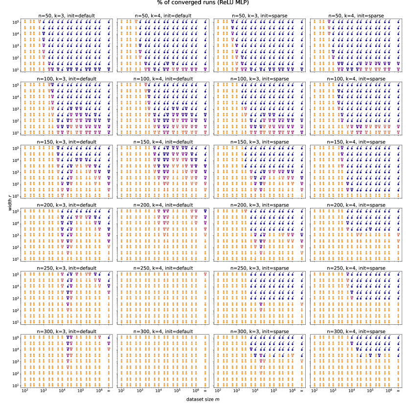
Figure 4: Full results for the sweep over dataset sizes and MLP widths. Each point represents $50$ independent training runs of a 2-layer ReLU MLP on the offline sparse parity problem (input dimension $n$, parity degree $k$, initialization scheme, width $r$, dataset size $m$). All other algorithmic choices (learning rate $\eta=0.1$, weight decay $\lambda=0.01$, batch size $B=32$, number of training iterations $T=10^{5}$) are kept the same. We note the following: (1) A success frontier, where wide networks can learn at small sample sizes $m\ll BT$ (far outside online regime); (2) Monotonic benefit of width: overparameterization does not worsen the failure mode of overfitting in this setting, and amplifies success probabilities; (3) Benefit of sparse axis-aligned initialization: for sufficiently large $n$ where default initialization no longer works, sparse initialization scheme enlarges the feasible regime; (4) Non-monotonic effects of dataset size: there are unpredictable failures as we vary $m$ (horizontal slices of these plots).

In our main set of large-scale synthetic experiments, we train a large number of 2-layer MLPs to solve various $(n,k)$-sparse parity problems, from $m$ samples. The full set of hyperparameters is listed below:

• Problem instance sizes: $n\in\{50,100,150,\ldots,300\}$, $k\in\{3,4\}$. Note that Barak et al., (2022) investigate empirical computational time scaling curves for larger $k$ (up to $8$) in the online ($m=\infty$) setting. We are able to observe convergence for larger $k$ in the offline setting, but we omit these results from the systematic grid sweep (the feasible regime is too small in terms of $n$).

• Dataset size: $m\in\{100,200,300,600,1000,2000,3000,\ldots,600000,1000000\}$. We also include runs in the online regime (rightmost columns in Figure 4), which correspond to the regime studied by Barak et al., (2022).

• Network width: $r\in\{10,30,100,300,\ldots,10000,30000,100000\}$.

• Initialization scheme: PyTorch default (uniform on the interval $[-1/\sqrt{n},1/\sqrt{n}]$), and random $2$-sparse rows. In coarser-grained hyperparameter searches, we found $2$ to be the optimal sparsity constant for large-width ($\geq 1000$) regimes studied in this paper; we do not fully understand why this is the case. We also keep the PyTorch default initialization scheme (uniform on the width-dependent interval $[-1/\sqrt{r},1/\sqrt{r}]$) for the second layer, and use default-initialized biases.

At each point in this hyperparameter space, we conduct $50$ training runs, and record the success probability, defined as the probability of achieving test error $\leq 10\%$ on a held-out sample of size $10^{4}$ within $T=10^{5}$ training iterations. The hyperparameters for SGD, selected via coarse-grained hyperparameter search to optimize for convergence time in the $n=200,k=3,r=10000$ setting, are as follows: minibatch size $B=32$; learning rate $\eta=0.1$; weight decay $\lambda=0.01$.

Figure 4 summarizes all of our runs, and overviews all of the findings (1) through (4) enumerated in the main paper. We go into more detail below:

1. A “success frontier”: large width can compensate for small datasets. We observe convergence and perfect generalization when $m\ll n^{k}$. In such regimes, which are far outside the online setting considered by Barak et al., (2022), high-probability sample-efficient learning is enabled by large width. Note that neither our theoretical or empirical results have sufficient granularity to predict or measure the precise way the smallest feasible sample size $m$ scales with the other size parameters (like $n,k,r$). The theoretical upper bounds show that if $r=\Omega(n^{k})$, idealized algorithms (modified for tractability of analysis) can obtain $O(\operatorname{poly}(n))$ or even $O(\log(n))$ sample complexity, and smaller $r$ can yield milder reductions of the exponent.

2. Width is monotonically beneficial, and buys data, time, and luck. Despite the capacity of wider neural networks to overfit larger datasets, we find that there are monotonic sample-efficiency benefits to increasing network width, in all of the hyperparameter settings considered in the grid sweep. This can be quickly quantitatively confirmed by starting at any point in Figure 4, and noting that success probabilities only increase going upwards (increasing $r$, keeping all other parameters equal). Along some of these vertical slices, we observe that transitions from $0\%$ to $100\%$ are present: at these corresponding dataset sizes $m$, large width makes sample-efficient learning possible. Figure 2 (center) shows this in greater detail, by choosing a denser grid of sample sizes $m$ near the empirical statistical limit.

3. Sparse axis-aligned initialization buys data, time, and luck. Used in conjunction with a wide network, we observe that a sparse, axis-aligned initialization scheme yields strong improvements on all of these axes. This can be seen by comparing the pairs of subplots in columns 1 vs. 3 and 2 vs. 4 in Figure 4. We found that $s=2$ (i.e. initialize every hidden-layer neuron with a random $2$-hot weight vector) works best for the settings considered in this study.

4. Intriguing effects of dataset size. Unlike the monotonicity along vertical slices in Figure 4, some of the horizontal slices exhibit non-monotonic success probabilities. Namely, as $m$ increases, keeping all else the same, the network enters and exits a first feasible regime; then, at large enough sample sizes (including the online setting), learning is observed to succeed again. Sparse initialization reduces this counterintuitive behavior, but not entirely (see, e.g., the $n=200,k=3$ cell). We do not attempt to explain this phenomenon; however, we found in preliminary investigations that the locations of the transitions are sensitive to the choice of weight decay hyperparameter. Figure 2 (right) shows this in greater detail, plotting median convergence times (as defined above) instead of success probabilities.

C.2 Lottery ticket subnetworks

Our theoretical analysis of sparse networks and experimental findings suggest that width provides a form of parallelization: wider networks have a higher probability of containing lucky neurons which have sufficient Fourier gaps at initialization to learn from the dataset. In Figure 5 we perform an experiment in the style of Frankle and Carbin, (2018), showing that indeed the neurons which end up being important in a wide sparsely-initialized network form an unusually lucky ‘winning ticket’ subnetwork. When we rewind the weights of this subnetwork to initialization, its test error starts out poor, but when we train just this subnetwork from initialization its performance quickly improves, unlike the large majority of randomly initialized subnetworks of the same size. For this experiment, batch size=32 and learning rate=0.1.

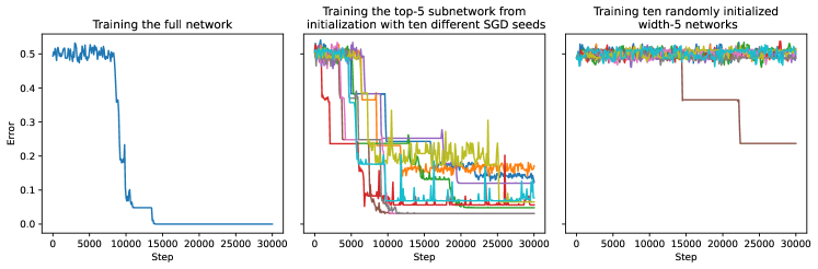
Figure 5: (Lottery tickets) Left: Training a width-100 MLP on the (n=50, k=5)-online sparse parity task, where each hidden neuron initialized with 2 non-zero incoming weights. Center: We prune all but the top 5 neurons by weight norm at the end of training; rewind weights to the original initialization, and retrain with various SGD random seeds. Right: The same as Center, but the weights are randomly reinitialized in each run.

C.3 Training wide & sparsely-initialized MLPs on natural tabular data

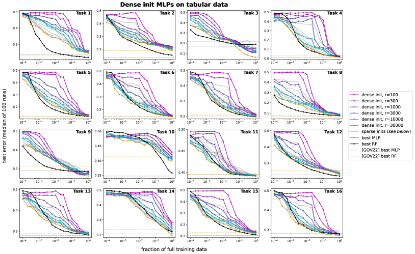
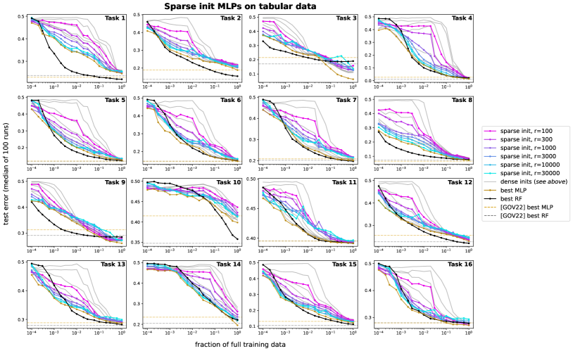
Figure 6: Full results of our tabular data experiments (following Grinsztajn et al., (2022)), varying MLP width $r$, sample size $m$ (via downsampling the training data), and initialization sparsity. Both width and sparsity tend to improve generalization, especially for small datasets. See Tables 1 and 2 for further details.

As a preliminary investigation of whether our findings translate well to realistic settings, we conduct experiments on the tabular benchmark curated by Grinsztajn et al., (2022). For simplicity, we use all 16 numerical classification tasks from the benchmark. These datasets originate from diverse domains such as health care, finance, and experimental physics. Our main comparison is between MLPs (with algorithmic choices inspired by our sparse parity findings) and random forests Breiman, (2001). We chose random forests as a baseline because they are known to achieve competitive performance with little tuning. Figure 6 summarizes our results, in which we find that wide and sparsely-initialized MLPs improve sample efficiency on small tabular datasets. We describe these experiments in full detail below.

Data preprocessing.

We standardize the dataset, centering each feature to have mean 0 and normalizing each feature to have standard deviation 1. For each task, we set aside 10% of the data for the test set, and downsample varying fractions of the remaining data to form a training set. We vary the downsampling fraction on an exponential grid: {1, 0.6, 0.3, 0.2, 0.1, 0.06, 0.03, 0.02, 0.01, 0.006, 0.003, 0.002, 0.001, 0.0006, 0.0003, 0.0002, 0.0001}. In each of 100 i.i.d. trials for each setting, we re-randomize the validation split as well as the downsampled training set.

Algorithms.

MLPs are trained using the same architectural choices noted in Section C.1, except the hyperparameters noted below. We use the scikit-learn Pedregosa et al., (2011) RandomForestClassifier. Hyperparameters not mentioned are set to library defaults.

Hyperparameter choices for MLPs.

• Width $r$: $\{100,300,1000,3000,10000,30000\}$. For deeper networks, the hidden layers are set to $r\times r$.

• Depth (number of hidden layers): $\{1,2,3\}$. In all of these settings, depth-$1$ networks are nearly uniformly outperformed by deeper ones of the same width.

• Sparsity of initialization: $s\in\{2,4\}$, and also dense (uniform) initialization. $4$-sparse initialization is nearly uniformly outperformed by $2$-sparse (in agreement with our experiments on sparse parity).

• Weight decay: $\{0,0.01\}$. In these settings, this hyperparameter had a minimal effect.

• Learning rate: $10^{-3}$

• Batch size: $256$

• Training epochs: $100$

Hyperparameter choices for RandomForestClassifier.

• max_depth: $\{-1,2,3,4,10\}$

• max_features: $\{1,2,3,4,\mathrm{sqrt},\mathrm{None}\}$

• n_estimators: $\{10,100,1000\}$

Larger widths.

For all of the tasks except 2 and 9 (since these are significantly larger datasets), we include extra runs with even larger networks: depth-2 MLPs with non-uniform width (i.e. sequence of hidden layer dimensions) $\{(100000,10000),(10000,100000)\}$.

Plots in Figure 6.

For clarity of presentation, in the plots where we vary MLP width and initialization sparsity, we fix depth to $3$ and sparsity level $s=2$. Qualitative trends are similar for other settings. The gold “best MLP” curves show the best median-of-100 validation losses across all architectures in the search space.

Comparison with full-data baselines.

To ensure that our baseline algorithm choices for MLPs and random forests are reasonable, we present a comparison with the results of Grinsztajn et al., (2022) (who performed extensive hyperparameter search) on the full datasets. These are shown as the dotted lines in Figure 6, as well as Table 2.

Task	OpenML identifier	# features	# examples
1	credit	11	16714
2	electricity	8	38474
3	covertype	11	566602
4	pol	27	10082
5	house_16H	17	13488
6	MagicTelescope	11	13376
7	bank-marketing	8	10578
8	MiniBooNE	51	72998
9	Higgs	25	940160
10	eye_movements	21	7608
11	Diabetes130US	8	71090
12	jannis	55	57580
13	default-of-credit-card-clients	21	13272
14	Bioresponse	420	3434
15	california	9	20634
16	heloc	23	10000

Table 1: Metadata for the 16 tabular classification benchmarks, curated by Grinsztajn et al., (2022) (January 2023 version, benchmark suite ID 337) and publicly available via OpenML.

Task	Best MLP			Best RF			(Grinsztajn et al.,, 2022)
	full	10%	1%	full	10%	1%	MLP	RF	Best model
1	24.5	27.8	34.2	22.0	22.9	24.8	22.9	23.6	22.5 (GBT)
2	18.9	23.2	25.1	15.4	18.0	23.0	23.6	13.7	12.8 (XGB)
3	6.3	13.7	23.2	19.1	18.9	21.4	21.6	17.1	17.1 (RF)
4	1.4	4.2	12.3	2.1	4.0	10.0	6.3	1.9	1.7 (XGB)
5	12.7	14.9	20.0	12.4	13.9	17.4	12.1	12.0	11.1 (XGB)
6	14.6	16.5	23.1	14.8	16.8	21.9	14.6	14.5	13.9 (FTT)
7	20.2	21.8	25.9	19.7	21.1	25.2	20.9	20.1	19.5 (GBT)
8	7.2	10.0	14.4	7.7	8.6	10.5	6.7	7.3	6.2 (XGB)
9	26.1	28.7	33.7	28.5	28.7	29.9	31.4	29.1	28.6 (XGB)
10	39.9	43.9	46.3	35.8	43.0	47.8	41.8	34.8	33.4 (XGB)
11	39.1	39.3	40.7	39.1	39.4	40.6	39.5	39.5	39.4 (XGB)
12	23.0	26.1	28.7	22.0	23.8	27.2	25.5	22.7	22.0 (XGB)
13	28.7	30.1	33.5	28.2	29.2	31.9	28.9	28.0	28.0 (RF)
14	19.5	28.9	37.6	22.2	29.2	39.8	23.4	20.5	20.5 (RF)
15	12.2	14.8	20.8	11.2	13.8	18.4	12.9	10.6	9.7 (XGB)
16	27.1	28.0	31.3	27.8	28.6	31.0	27.8	28.1	27.4 (ResNet)

Table 2: Numerical comparisons for the tabular data experiments, to accompany Figure 6. We report the median test error (%) over 100 i.i.d. training runs of MLPs and random forests. The 3 subcolumns in each group denote models trained on the full dataset and their {10%, 1%} downsampled counterparts. For all of these results, bootstrap $95\%$ confidence intervals have width $<2\%$. We observe that wide and/or sparsely-initialized MLPs are competitive with tree-based methods. In the rightmost 3 columns, we provide test errors for the same tasks, reported by (Grinsztajn et al.,, 2022) (GBT = gradient boosted tree, XGB = XGBoost, FTT = Feature Tokenizer + Transformer (Gorishniy et al.,, 2021)). Note that our cross-validation protocol differs slightly (to handle variance incurred by downsampling), which may explain performance discrepancies. We include these only to illustrate that our full-data accuracies are commensurate with those in prior works focused exclusively on benchmarking models for tabular data.

Results.

We note the following findings from the results in Figure 6 and Table 2:

• Wide networks resist overfitting on small tabular datasets. Like in the synthetic experiments, width yields monotonic end-to-end benefits for sample-efficient learning on these datasets. This suggests that the “parallel search + pruning” mechanisms analyzed in our paper are empirically at play in these settings, and that these networks’ capacity to overfit does not preclude nontrivial feature learning and generalization. These comparisons can be seen by comparing the colored curves (which represent depths $2$ and $3$) within each subplot in Figure 6. In some (but not all) cases, these MLPs perform competitively with hyperparameter-tuned random forest classifiers.

• Sparse axis-aligned initialization sometimes improves end-to-end performance. These comparisons can be seen by comparing vertically adjacent sparse vs. dense subplots in Figure 6. This effect is especially pronounced on datasets which are downsampled to be orders of magnitude smaller. We believe that this class of drop-in replacements for standard initialization merits further investigation, and may contribute to closing the remaining performance gap between deep learning and tree ensembles on small tabular datasets.

C.4 Software, compute infrastructure, and resource costs

GPU-accelerated training and evaluation pipelines were implemented in PyTorch (Paszke et al.,, 2019). Each training run was performed on one GPU in an internal cluster, with NVIDIA P40, P100, V100, and RTX A6000 GPUs. A single $T=10^{5}$ training run took 10 seconds on average (with early termination for the vast majority of grid sweeps); across all of the results in this paper, around $2\times 10^{5}$ training runs were performed, in a total of $600$ GPU-hours. Note that the precise evaluation of test error (at batch size $10^{4}$) constitutes a significant portion of the computational cost; this necessitated mindful GPU parallelization.

References

- Abbe et al., (2022) Abbe, E., Adsera, E. B., and Misiakiewicz, T. (2022). The merged-staircase property: a necessary and nearly sufficient condition for sgd learning of sparse functions on two-layer neural networks. In Conference on Learning Theory, pages 4782–4887. PMLR.
- Abbe et al., (2023) Abbe, E., Boix-Adsera, E., and Misiakiewicz, T. (2023). Sgd learning on neural networks: leap complexity and saddle-to-saddle dynamics. arXiv preprint arXiv:2302.11055.
- Andoni et al., (2014) Andoni, A., Panigrahy, R., Valiant, G., and Zhang, L. (2014). Learning polynomials with neural networks. In International Conference on Machine Learning, pages 1908–1916. PMLR.
- Applebaum et al., (2010) Applebaum, B., Barak, B., and Wigderson, A. (2010). Public-key cryptography from different assumptions. In Proceedings of the forty-second ACM symposium on Theory of computing, pages 171–180.
- Applebaum et al., (2009) Applebaum, B., Cash, D., Peikert, C., and Sahai, A. (2009). Fast cryptographic primitives and circular-secure encryption based on hard learning problems. In Annual International Cryptology Conference, pages 595–618. Springer.
- Ba et al., (2022) Ba, J., Erdogdu, M. A., Suzuki, T., Wang, Z., Wu, D., and Yang, G. (2022). High-dimensional asymptotics of feature learning: How one gradient step improves the representation. Advances in Neural Information Processing Systems, 35:37932–37946.
- Bachmann et al., (2023) Bachmann, G., Anagnostidis, S., and Hofmann, T. (2023). Scaling mlps: A tale of inductive bias. arXiv preprint arXiv:2306.13575.
- Bahri et al., (2021) Bahri, Y., Dyer, E., Kaplan, J., Lee, J., and Sharma, U. (2021). Explaining neural scaling laws. arXiv preprint arXiv:2102.06701.
- Barak et al., (2022) Barak, B., Edelman, B., Goel, S., Kakade, S., Malach, E., and Zhang, C. (2022). Hidden progress in deep learning: Sgd learns parities near the computational limit. Advances in Neural Information Processing Systems, 35:21750–21764.
- Ben Arous et al., (2021) Ben Arous, G., Gheissari, R., and Jagannath, A. (2021). Online stochastic gradient descent on non-convex losses from high-dimensional inference. The Journal of Machine Learning Research, 22(1):4788–4838.
- Bietti et al., (2022) Bietti, A., Bruna, J., Sanford, C., and Song, M. J. (2022). Learning single-index models with shallow neural networks. Advances in Neural Information Processing Systems, 35:9768–9783.
- Blum et al., (1994) Blum, A., Furst, M., Jackson, J., Kearns, M., Mansour, Y., and Rudich, S. (1994). Weakly learning dnf and characterizing statistical query learning using fourier analysis. In Proceedings of the twenty-sixth annual ACM symposium on Theory of computing, pages 253–262.
- Blum et al., (2003) Blum, A., Kalai, A., and Wasserman, H. (2003). Noise-tolerant learning, the parity problem, and the statistical query model. Journal of the ACM (JACM), 50(4):506–519.
- Borisov et al., (2022) Borisov, V., Leemann, T., Seßler, K., Haug, J., Pawelczyk, M., and Kasneci, G. (2022). Deep neural networks and tabular data: A survey. IEEE Transactions on Neural Networks and Learning Systems.
- Breiman, (2001) Breiman, L. (2001). Random forests. Machine learning, 45:5–32.
- Chen and Meka, (2020) Chen, S. and Meka, R. (2020). Learning polynomials in few relevant dimensions. In Conference on Learning Theory, pages 1161–1227. PMLR.
- Chen and Guestrin, (2016) Chen, T. and Guestrin, C. (2016). Xgboost: A scalable tree boosting system. In Proceedings of the 22nd acm sigkdd international conference on knowledge discovery and data mining, pages 785–794.
- Chizat et al., (2019) Chizat, L., Oyallon, E., and Bach, F. (2019). On lazy training in differentiable programming. Advances in neural information processing systems, 32.
- Damian et al., (2022) Damian, A., Lee, J., and Soltanolkotabi, M. (2022). Neural networks can learn representations with gradient descent. In Conference on Learning Theory, pages 5413–5452. PMLR.
- Damian et al., (2023) Damian, A., Nichani, E., Ge, R., and Lee, J. D. (2023). Smoothing the landscape boosts the signal for sgd: Optimal sample complexity for learning single index models. arXiv preprint arXiv:2305.10633.
- Daniely and Malach, (2020) Daniely, A. and Malach, E. (2020). Learning parities with neural networks. Advances in Neural Information Processing Systems, 33:20356–20365.
- Dosovitskiy et al., (2020) Dosovitskiy, A., Beyer, L., Kolesnikov, A., Weissenborn, D., Zhai, X., Unterthiner, T., Dehghani, M., Minderer, M., Heigold, G., Gelly, S., et al. (2020). An image is worth 16x16 words: Transformers for image recognition at scale. arXiv preprint arXiv:2010.11929.
- Du et al., (2018) Du, S. S., Zhai, X., Poczos, B., and Singh, A. (2018). Gradient descent provably optimizes over-parameterized neural networks. arXiv preprint arXiv:1810.02054.
- Feldman, (2008) Feldman, V. (2008). Evolvability from learning algorithms. In Proceedings of the fortieth annual ACM symposium on Theory of computing, pages 619–628.
- Feldman et al., (2017) Feldman, V., Guzman, C., and Vempala, S. (2017). Statistical query algorithms for mean vector estimation and stochastic convex optimization. In Proceedings of the Twenty-Eighth Annual ACM-SIAM Symposium on Discrete Algorithms, pages 1265–1277. SIAM.
- Frankle and Carbin, (2018) Frankle, J. and Carbin, M. (2018). The lottery ticket hypothesis: Finding sparse, trainable neural networks. arXiv preprint arXiv:1803.03635.
- Frei et al., (2022) Frei, S., Chatterji, N. S., and Bartlett, P. L. (2022). Random feature amplification: Feature learning and generalization in neural networks. arXiv preprint arXiv:2202.07626.
- Gorishniy et al., (2021) Gorishniy, Y., Rubachev, I., Khrulkov, V., and Babenko, A. (2021). Revisiting deep learning models for tabular data. Advances in Neural Information Processing Systems, 34:18932–18943.
- Grinsztajn et al., (2022) Grinsztajn, L., Oyallon, E., and Varoquaux, G. (2022). Why do tree-based models still outperform deep learning on typical tabular data? In Koyejo, S., Mohamed, S., Agarwal, A., Belgrave, D., Cho, K., and Oh, A., editors, Advances in Neural Information Processing Systems, volume 35, pages 507–520. Curran Associates, Inc.
- Hahn, (2020) Hahn, M. (2020). Theoretical limitations of self-attention in neural sequence models. Transactions of the Association for Computational Linguistics, 8:156–171.
- Henighan et al., (2020) Henighan, T., Kaplan, J., Katz, M., Chen, M., Hesse, C., Jackson, J., Jun, H., Brown, T. B., Dhariwal, P., Gray, S., et al. (2020). Scaling laws for autoregressive generative modeling. arXiv preprint arXiv:2010.14701.
- Hoffmann et al., (2022) Hoffmann, J., Borgeaud, S., Mensch, A., Buchatskaya, E., Cai, T., Rutherford, E., Casas, D. d. L., Hendricks, L. A., Welbl, J., Clark, A., et al. (2022). Training compute-optimal large language models. arXiv preprint arXiv:2203.15556.
- Hutter, (2021) Hutter, M. (2021). Learning curve theory. arXiv preprint arXiv:2102.04074.
- Jacot et al., (2018) Jacot, A., Gabriel, F., and Hongler, C. (2018). Neural tangent kernel: Convergence and generalization in neural networks. Advances in neural information processing systems, 31.
- Kaggle, (2021) Kaggle (2021). State of data science and machine learning 2021.
- Kamath et al., (2020) Kamath, P., Montasser, O., and Srebro, N. (2020). Approximate is good enough: Probabilistic variants of dimensional and margin complexity. In Conference on Learning Theory, pages 2236–2262. PMLR.
- Kaplan et al., (2020) Kaplan, J., McCandlish, S., Henighan, T., Brown, T. B., Chess, B., Child, R., Gray, S., Radford, A., Wu, J., and Amodei, D. (2020). Scaling laws for neural language models. arXiv preprint arXiv:2001.08361.
- Kearns, (1998) Kearns, M. (1998). Efficient noise-tolerant learning from statistical queries. Journal of the ACM (JACM), 45(6):983–1006.
- Kol et al., (2017) Kol, G., Raz, R., and Tal, A. (2017). Time-space hardness of learning sparse parities. In Proceedings of the 49th Annual ACM SIGACT Symposium on Theory of Computing, pages 1067–1080.
- Liu et al., (2022) Liu, Z., Michaud, E. J., and Tegmark, M. (2022). Omnigrok: Grokking beyond algorithmic data. arXiv preprint arXiv:2210.01117.
- Lutz et al., (2022) Lutz, P., Arnould, L., Boyer, C., and Scornet, E. (2022). Sparse tree-based initialization for neural networks. arXiv preprint arXiv:2209.15283.
- Malach et al., (2021) Malach, E., Kamath, P., Abbe, E., and Srebro, N. (2021). Quantifying the benefit of using differentiable learning over tangent kernels. In International Conference on Machine Learning, pages 7379–7389. PMLR.
- Merrill et al., (2023) Merrill, W., Tsilivis, N., and Shukla, A. (2023). A tale of two circuits: Grokking as competition of sparse and dense subnetworks. arXiv preprint arXiv:2303.11873.
- Michaud et al., (2023) Michaud, E. J., Liu, Z., Girit, U., and Tegmark, M. (2023). The quantization model of neural scaling. arXiv preprint arXiv:2303.13506.
- Minsky and Papert, (1969) Minsky, M. and Papert, S. (1969). Perceptrons: an introduction to computational geometry. MIT Press.
- Nakkiran et al., (2021) Nakkiran, P., Kaplun, G., Bansal, Y., Yang, T., Barak, B., and Sutskever, I. (2021). Deep double descent: Where bigger models and more data hurt. Journal of Statistical Mechanics: Theory and Experiment, 2021(12):124003.
- O’Donnell, (2014) O’Donnell, R. (2014). Analysis of Boolean functions. Cambridge University Press.
- Paszke et al., (2019) Paszke, A., Gross, S., Massa, F., Lerer, A., Bradbury, J., Chanan, G., Killeen, T., Lin, Z., Gimelshein, N., Antiga, L., Desmaison, A., Kopf, A., Yang, E., DeVito, Z., Raison, M., Tejani, A., Chilamkurthy, S., Steiner, B., Fang, L., Bai, J., and Chintala, S. (2019). PyTorch: An imperative style, high-performance deep learning library. In Wallach, H., Larochelle, H., Beygelzimer, A., d'Alché-Buc, F., Fox, E., and Garnett, R., editors, Advances in Neural Information Processing Systems 32, pages 8024–8035. Curran Associates, Inc.
- Pedregosa et al., (2011) Pedregosa, F., Varoquaux, G., Gramfort, A., Michel, V., Thirion, B., Grisel, O., Blondel, M., Prettenhofer, P., Weiss, R., Dubourg, V., Vanderplas, J., Passos, A., Cournapeau, D., Brucher, M., Perrot, M., and Duchesnay, E. (2011). Scikit-learn: Machine learning in Python. Journal of Machine Learning Research, 12:2825–2830.
- Power et al., (2022) Power, A., Burda, Y., Edwards, H., Babuschkin, I., and Misra, V. (2022). Grokking: Generalization beyond overfitting on small algorithmic datasets. arXiv preprint arXiv:2201.02177.
- Rosen-Zvi et al., (2002) Rosen-Zvi, M., Klein, E., Kanter, I., and Kinzel, W. (2002). Mutual learning in a tree parity machine and its application to cryptography. Physical Review E, 66(6):066135.
- Shalev-Shwartz and Ben-David, (2014) Shalev-Shwartz, S. and Ben-David, S. (2014). Understanding machine learning: From theory to algorithms. Cambridge university press.
- Shalev-Shwartz et al., (2017) Shalev-Shwartz, S., Shamir, O., and Shammah, S. (2017). Failures of gradient-based deep learning. In International Conference on Machine Learning, pages 3067–3075. PMLR.
- Shamir and Zhang, (2013) Shamir, O. and Zhang, T. (2013). Stochastic gradient descent for non-smooth optimization: Convergence results and optimal averaging schemes. In International conference on machine learning, pages 71–79. PMLR.
- Shi et al., (2021) Shi, Z., Wei, J., and Liang, Y. (2021). A theoretical analysis on feature learning in neural networks: Emergence from inputs and advantage over fixed features. In International Conference on Learning Representations.
- Telgarsky, (2022) Telgarsky, M. (2022). Feature selection with gradient descent on two-layer networks in low-rotation regimes. arXiv preprint arXiv:2208.02789.
- Tolstikhin et al., (2021) Tolstikhin, I. O., Houlsby, N., Kolesnikov, A., Beyer, L., Zhai, X., Unterthiner, T., Yung, J., Steiner, A., Keysers, D., Uszkoreit, J., et al. (2021). MLP-Mixer: An all-MLP architecture for vision. Advances in neural information processing systems, 34:24261–24272.
- Wei et al., (2019) Wei, C., Lee, J. D., Liu, Q., and Ma, T. (2019). Regularization matters: Generalization and optimization of neural nets vs their induced kernel. Advances in Neural Information Processing Systems, 32.
- (59) Yang, G., Hu, E. J., Babuschkin, I., Sidor, S., Liu, X., Farhi, D., Ryder, N., Pachocki, J., Chen, W., and Gao, J. (2022a). Tensor programs v: Tuning large neural networks via zero-shot hyperparameter transfer. arXiv preprint arXiv:2203.03466.
- (60) Yang, J., Lindenbaum, O., and Kluger, Y. (2022b). Locally sparse neural networks for tabular biomedical data. In International Conference on Machine Learning, pages 25123–25153. PMLR.
- Zhai et al., (2022) Zhai, X., Kolesnikov, A., Houlsby, N., and Beyer, L. (2022). Scaling vision transformers. In Proceedings of the IEEE/CVF Conference on Computer Vision and Pattern Recognition, pages 12104–12113.
- Zhenmei et al., (2022) Zhenmei, S., Wei, J., and Liang, Y. (2022). A theoretical analysis on feature learning in neural networks: Emergence from inputs and advantage over fixed features. In International Conference on Learning Representations.