Data-Adaptive Graph Framelets with Generalized Vanishing Moments for Graph Signal Processing

Abstract

In this paper, we propose a novel and general framework to construct tight framelet systems on graphs with localized supports based on hierarchical partitions. Our construction provides parametrized graph framelet systems with great generality based on partition trees, by which we are able to find the size of a low-dimensional subspace that best fits the low-rank structure of a family of signals. The orthogonal decomposition of subspaces provides a key ingredient for the definition of “generalized vanishing moments” for graph framelets. In a data-adaptive setting, the graph framelet systems can be learned by solving an optimization problem on Stiefel manifolds with respect to our parameterization. Moreover, such graph framelet systems can be further improved by solving a subsequent optimization problem on Stiefel manifolds, aiming at providing the utmost sparsity for a given family of graph signals. Experimental results show that our learned graph framelet systems perform superiorly in non-linear approximation and denoising tasks.

I Introduction and Motivation

Graphs are prevalent data formats that have a variety of realizations in real life, e.g., social networks, traffic networks, sensor networks, etc. Given its practical importance, it is desired to have efficient signal processing tools on graphs, and the area of graph signal processing (GSP) has been one of the most active research areas during the past decade [1, 2]. Compared with signals, images, and other Euclidean-type data, graph data/signals are more irregular and flexible. Therefore, classical signal processing methods can not directly be applied to such data. In graph signal processing, a central topic is to develop notions and tools that resemble those on the continuous spaces or the discrete $d$-dimensional ($d$-D) signals, e.g., the Fourier and wavelet/framelet transforms. Stemmed from the spectral graph theory [3], the graph Fourier transforms (GFTs) based on graph Laplacians are by far one of the most fundamental concepts/tools upon which many other tools are developed.

By GFTs, notions of frequencies, low-pass filters, and high-pass filters can be defined similarly to those of the Euclidean counterparts. These concepts further facilitate the development of an analysis-synthesis framework using two-channel filtersbanks and up/down samplings on graphs analog to classical 1-D cases. The work in [4] shows that this can be established on bipartite graphs, on which up/down sampling is the simple restriction on either set of the bi-partition. This is essentially due to the algebraic property of spectral folding that is satisfied on the bipartite graphs. For arbitrary graphs, this property is not guaranteed, and one way to tackle this issue is to decompose the original graph into bipartite subgraphs. The graph signal processing is then conducted on each bipartite subgraph independently. Subsequent work improves [4] from the following aspects: (1) Using compact (polynomial) and biorthogonal filters by allowing different filter banks in the analysis and synthesis phases [5]. (2) Applying over-sampled bipartite graphs since the algorithm of decomposition in bipartite subgraphs in [4] results in a loss of edges of the original graphs [6]. (3) Improving computational complexity and quality of down samplings from using maximum spanning trees [7, 8]. (4) Generalizations to arbitrary graphs by applying generalized sampling operators, generalized graph Laplacians, and generalized inner-products [9, 10]. All of these have shown certain capabilities among various graph signal processing tasks.

Apart from the aforementioned work, there are many other realizations of graph signal analysis-synthesis tools based on various motivations and possessing other types of characteristics and merits [11, 12, 13, 14, 15, 16, 17, 18]. From a general perspective, we can unify these GSP approaches by viewing graph signals as vectors in $\mathbb{R}^{n}$ and one is aiming at the construction of representation systems for graph signals have various desired properties. The analysis and synthesis phases with respect to a representation system are typically corresponding to two matrices $\bm{T}_{a}$ and $\bm{T}_{s}$, respectively. One of the most important properties of a graph signal representation system is the perfect reconstruction property, i.e., $\bm{T}_{s}\bm{T}_{a}=\bm{I}$ with $\bm{I}$ being the identity matrix of a certain size. The property of critical sampling, i.e., $\bm{T}_{a},\bm{T}_{s}\in\mathbb{R}^{n\times n}$, is also desirable in some applications such as the graph signal compression. The perfect reconstruction allows for recovering the signal after decomposition, while the critical sampling indicates that compared with the original signal, there is no extra storage overhead after analysis.

However, critical sampling could be a drawback in some other applications. For example, in graph signal denoising, redundancy plays a crucial role in exploiting the intrinsic structures of the underlying noisy signal. By constructing systems with $\bm{T}_{a}$ as a redundant frame operator to represent graph signals rather than a non-redundant basis, one can generate smaller coefficients from such a system for noisy signals and therefore, the portions of noise have a larger chance to be thresholded. Moreover, in terms of tightness of the representation systems, except for special cases in [4, 12, 13], in the other aforementioned work, $\bm{T}_{s}\neq\bm{T}_{a}^{\top}$ (the transpose of $\bm{T}_{a}$) and thus we can not represent the analysis-synthesis framework using only $\bm{T}_{a}$. The tightness of the representation system requires the construction of $\bm{T}_{a}$ and $\bm{T}_{s}$ such that $\bm{T}_{s}=\bm{T}_{a}^{\top}$, $\bm{T}_{a}^{\top}\bm{T}_{a}=\bm{I}$ with $\bm{T}_{a}\in\mathbb{R}^{m\times n}$ for some $m\geq n$, which is equivalent to require that the rows of $\bm{T}_{a}$ forms a tight frame on $\mathbb{R}^{n}$. There are a few existing work [19, 20, 21, 22, 23] on tight frames for graph signal representations, most of which are derived from GFTs and thus are called spectral wavelets/framelets [19]. While spectral wavelets/framelets are well-interpreted in the frequency domain, the wavelets/framelets generally do not have localized support unless the filters are polynomial-type. In this case, $\bm{T}_{a}$ is a dense matrix which leads to computation and storage burden. To facilitate efficient computations, polynomial approximations to the target filters are applied. But then it fails to be a tight frame, i.e. $\bm{T}^{\top}_{a}\bm{T}_{a}\neq\bm{I}$[19]. On the other hand, following [24, 25, 26, 27] that utilize a series of hierarchical partitions on graphs, a recent work [28] proposes Haar-type graph framelets with localized support.

Sparsity is one of the key characteristics for achieving efficient and effective signal processing since it implies the capability of representing signals with significantly fewer coefficients. A typical way to achieve sparsity in classical $d$-D discrete wavelet/framelet transforms is to construct high-pass filters with high vanishing moments [29, Sec. 1.2]. To elaborate, since smooth functions can be approximated by polynomials (using the Taylor expansion), polynomial sequences convolving with a filter with high vanishing moments vanish up to a certain order, and thus, the wavelet/framelet (high-pass filter) coefficients of the discrete samples of smooth functions are consequently very sparse. The theory for classical wavelet/framelet analysis is well-established; see, e.g., [30, 29, 31]. For more complicated families of signals, wavelets/framelets with more desirable properties than those of the ordinary wavelets, for example, the directionality, are required in order to achieve (optimal) sparsity for the representations of specific families of signals [32, 33, 34, 35, 36, 37, 38, 39]. On the contrary, it is generally difficult to define the corresponding notions of vanishing moments, smooth functions, and approximation properties for signals on graphs due to the irregular structure of graphs. It is also difficult to define families of signals of graphs with special properties, e.g. directional signals on graphs.

Therefore, it is plausible why sparsity is seldom theoretically discussed in graph signal processing. However, there are still some attempts to define generalized vanishing moments for graphs. In [40], the property of being orthogonal to the first $k$ graph Laplacian eigenvectors is regarded as having generalized $k$ vanishing moments. A graph wavelet system is subsequently defined and the wavelets are guaranteed to have this property. For signals that are well approximated by the first $k$ eigenvectors, the system is able to produce very sparse coefficients. This inspires us to consider a more general construction of graph framelet systems in which a family of signals is not assumed to be well-approximated by the first $k$ eigenvectors but still largely lying in a $k$-dimensional subspace. Similarly, the orthogonality with this subspace can also be considered as having generalized vanishing moments and a system with this property is able to produce sparse coefficients for the family of signals. Hence, we seek to learn the low-dimensional structure of the family and construct graph framelet systems having such generalized vanishing moments. This resembles training a model in a machine learning task and can be regarded as a data-adaptive approach for the construction of graph framelet systems.

To achieve this goal, we propose a parametrized frame on graphs that generalizes previous work. As in [28], our systems are based on a partition tree that consists of a series of hierarchical partitions of the graph. Consequently, the constructed graph framelets are localized and fast transform algorithms are realizable. With the parametrization, our proposed graph framelet systems possess novel mathematical generality that includes [28] and [12] as special cases. Moreover, we propose to learn a low-dimensional subspace for a family of signals, in which we find a set of orthonormal vectors that fits a set of sample signals optimally in the $l^{2}$ sense. In such a way, our systems are expected to sparsely represent the given family of signals since the graph framelets in our system are orthogonal to this subspace. This system is further optimized so as to obtain the utmost sparsity in representing the given family of signals. The parameterization of our system is actually on the Stiefel manifolds and can be solved through two smooth optimization problems using the conjugate gradient method on the Riemannian manifolds. The graph framelets in our system thus have generalized vanishing moments and are capable of representing the given family of signals sparsely.

To summarize, the contribution of this paper is as follows:

1. We propose a novel, general, and fully parametrized method to construct tight frames on graphs, in which the graph framelets are with localized support and realizable fast transform algorithms.

2. We propose using our parameterized system to learn the low-dimensional structure of a given family of graph signals so that the resulting graph framelets possess generalized vanishing moments facilitating sparse representation.

3. We conduct the learning by solving two Riemannian optimization problems on the Stiefel manifolds to obtain the data-adaptive graph framelet systems.

4. We demonstrate the effectiveness of our proposed method by comparing it with other approaches in non-linear approximation and denoising tasks in graph signal processing.

The rest of this paper is organized as follows. The construction of $\mathcal{V}$-framelet and $\mathcal{G}$-framelet systems are described in Section II. The graph framelet transforms and their computational complexities are discussed in Section III. Data-adaptive realizations of the graph framelet systems based on Stiefel manifold optimizations are detailed in Section IV. In Section V, numerical experiments and comparisons are conducted for the tasks of non-linear approximation and denoising in graph signal processing. Conclusion and final remarks are given in Section VI.

II Graph Framelet Systems

In this section, we focus on the detailed construction of general graph framelet systems and the characterizations of such systems to be tight frames. Moreover, such framelet systems can enjoy desirable properties such as localized supports, generalized vanishing moments, fast transform algorithms, and so on.

II-A Preliminaries

We first introduce some necessary notation, definitions, and preliminary results. We denote an undirected weighted graph with $n$ vertices as $\mathcal{G}:=(\mathcal{V},\mathcal{E},\bm{W})$ (or simply $\mathcal{G}:=(\mathcal{V},\mathcal{E})$), where $\mathcal{V}:=\{v_{1},v_{2},\dots,v_{n}\}$, $\mathcal{E}\subset\mathcal{V}\times\mathcal{V}$, $\bm{W}=(w_{ij})_{1\leq i,j\leq n}\in\mathbb{R}^{n\times n}$ denote the set of vertices, the set of edges, and the weight (adjacency) matrix, respectively. The space $L^{2}(\mathcal{G}):=\{f\,|\,\mathcal{V}\rightarrow\mathbb{R}\}$ is the collection of graph signals on $\mathcal{G}$ and can be regarded as the finite-dimensional Hilbert space $\mathbb{R}^{n}$ with the usual Euclidean inner-product $\langle\cdot,\cdot\rangle$ and induced norm $\|\cdot\|:=\sqrt{\langle\cdot,\cdot\rangle}$. The cardinality of a set is denoted by $|\cdot|$. Let $\bm{L}:=\bm{D}-\bm{W}$ denote the unnormalized graph Laplacian matrix, where the diagonal matrix $\bm{D}:=\text{diag}(d_{1},d_{2},\dots,d_{n})$ with $d_{i}:=\sum_{j=1}^{n}w_{ij},1\leq i\leq n$ is the degree matrix. $\bm{L}$ is positive semidefinite and thus it has $n$ eigenvalues $0\leq\lambda_{1}\leq\lambda_{2}\leq\dots\leq\lambda_{n}$ associated with real orthonormal eigenvectors $\bm{u}_{1},\bm{u}_{2},\dots,\bm{u}_{n}$. If $\mathcal{G}$ is connected, than $\bm{u}_{1}$ a vector with constant element $1/\sqrt{n}$.

For $K\in\mathbb{N}$, the set $\{1,\dots,K\}$ is denoted as $[K]$. For a matrix $\bm{M}$, we denote its $i$-th row as $\bm{M}_{i,:}$. We denote $\bm{I}$ the identity matrix of a certain size and omit its size for simplicity. Vectors in $\mathbb{R}^{d},d\in\mathbb{N}$ are assumed to be row vectors, or equivalently matrices in $\mathbb{R}^{1\times d}$. Given a set $\{\bm{X}_{i}\}_{i=1}^{m}\subseteq\mathbb{R}^{s\times t}$ of $m$ matrices, we use $\mathrm{CONCAT}(\{\bm{X}_{i}\}_{i=1}^{m}):=\llbracket\bm{X}_{i}\rrbracket_{i\in[m]}:=[\bm{X}_{1}^{\top},\ldots,\bm{X}_{m}^{\top}]^{\top}$ to denote the matrix in $\mathbb{R}^{ms\times t}$ constructed by concatenating $\bm{X}_{1},\bm{X}_{2},\dots,\bm{X}_{m}$ along the rows. We also use $\bm{\llparenthesis}\bm{X}_{i}\bm{\rrparenthesis}_{i\in[m]}:=[\bm{X}_{1},\ldots,\bm{X}_{m}]\in\mathbb{R}^{s\times mt}$ to denote concatenation along the columns. For $\bm{X}\in\mathbb{R}^{m\times d}$, we use $\mathrm{VEC}(\bm{X})$ to denote the vector in $\mathbb{R}^{md}$ constructed by concatenating the rows $\bm{X}_{i,:},1\leq i\leq m$. For $\bm{x}\in\mathbb{R}^{md}$, we use $\mathrm{MAT}(\bm{x},m)$ to denote the inverse of VEC, i.e. constructing a matrix $\bm{X}\in\mathbb{R}^{m\times d}$ from the vector $\bm{x}$ by consecutively slicing $\bm{x}$ into $m$ vectors in $\mathbb{R}^{d}$ and concatenating them along the rows. We use $\lceil\cdot\rceil$ to denote the ceiling operation of real numbers.

A countable set $\{\phi_{i}\}_{i\in\mathcal{I}}$ of a real Hilbert space $\mathcal{H}$ is called a tight frame of $\mathcal{H}$ if and only if

$$\|f\|^{2}_{\mathcal{H}}=\sum_{i\in\mathcal{I}}|\langle f,\phi_{i}\rangle_{\mathcal{H}}|^{2},\quad\forall f\in\mathcal{H},$$

where $\langle\cdot,\cdot\rangle_{\mathcal{H}},\|\cdot\|_{\mathcal{H}}$ are the inner-product and the induced norm on $\mathcal{H}$, respectively. The condition above is equivalent to

$$f=\sum_{i\in\mathcal{I}}\langle f,\phi_{i}\rangle_{\mathcal{H}}\phi_{i},\quad\forall f\in\mathcal{H}.$$ (1)

Thus, we can decompose and reconstruct any $f\in\mathcal{H}$ using $\{\phi_{i}\}_{i\in\mathcal{I}}$ alone. The focus of this paper is to construct tight graph framelet systems for $\mathcal{H}=L^{2}(\mathcal{G})$.

Under an abuse of notation, we regard $\mathrm{span}(\bm{X})$ as the span of the row vectors of a matrix $\bm{X}$. We have the following key lemma concerning the characterization of the span of a matrix.

Lemma 1.

Let $\bm{X}:=\llbracket\bm{\xi}_{i}\rrbracket_{i\in[m]}\in\mathbb{R}^{m\times n}$ be defined from the set $\{\bm{\xi}_{i}\}_{i=1}^{m}$ of orthonormal row vectors in $\mathbb{R}^{n}$. Let $\bm{A}\in\mathbb{R}^{m_{1}\times m}$ and $\bm{B}\in\mathbb{R}^{m_{2}\times m}$ be two matrices such that $1\leq m_{1}<m$. Define $\bm{\Phi}:=\llbracket\bm{\varphi}_{i}\rrbracket_{i\in[m_{1}]}:=\bm{A}\bm{X}$ and $\bm{\Psi}:=\llbracket\bm{\psi}_{i}\rrbracket_{i\in[m_{2}]}:=\bm{B}\bm{X}$. Then the following two statements are equivalent.

• The matrices $\bm{A}$ and $\bm{B}$ satisfy $\bm{A}\bm{A}^{\top}=\bm{I}$, $\bm{B}\bm{A}^{\top}=\bm{0}$, and $\text{{rank}}(\bm{B})=m-m_{1}$.

• $\mathrm{span}(\bm{X})=\mathrm{span}(\bm{\Phi})\oplus\mathrm{span}(\bm{\Psi})$ and the set $\{\bm{\varphi}_{i}\}_{i\in[m_{1}]}$ is an orthonormnal basis for $\mathrm{span}(\bm{\Phi})$.

Moreover, with the additional assumption of either (a) or (b), the following statements are equivalent.

• $\bm{A}^{\top}\bm{A}+\bm{B}^{\top}\bm{B}=\bm{I}$.

• $\bm{\Phi}^{\top}\bm{\Phi}+\bm{\Psi}^{\top}\bm{\Psi}=\bm{X}^{\top}\bm{X}$.

• $\bm{B}\bm{B}^{\top}\bm{B}=\bm{B}$.

• $\{\bm{\psi}_{i}\}_{i\in[m_{2}]}$ is a tight frame of $\mathrm{span}(\bm{\Psi})$.

Proof.

It is obvious that (a)$\Rightarrow$(b). For (b)$\Rightarrow$(a), in view of $\bm{X}\bm{X}^{\top}=\bm{I}$ and $\bm{\Phi}\bm{\Phi}^{\top}=\bm{I}$, we have $\bm{A}\bm{A}^{\top}=\bm{I}$. The condition $\bm{B}\bm{A}^{\top}=\bm{0}$ follows from $\mathrm{span}(\bm{\Psi})\perp\mathrm{span}(\bm{\Phi})$. By the isomorphism between $\mathbb{R}^{m}$ and $\mathrm{span}(\bm{X})=\mathrm{span}(\bm{\Phi})\oplus\mathrm{span}(\bm{\Psi})$, we deduce that $\mathbb{R}^{m}=\mathrm{span}(\bm{A})\oplus\mathrm{span}(\bm{B})$, which implies the full rank condition $\mathrm{rank}(B)=m-m_{1}$ of $\bm{B}$. Hence (b)$\Rightarrow$(a). Consequently, (a)$\Leftrightarrow$(b).

Now suppose (a) holds. We next prove that (i) – (iv) are equivalent. In fact, the equivalence between (i) and (ii) is obvious. From [41, Lemma 1], we see that $\bm{B}\bm{B}^{\top}\bm{B}=\bm{B}$ is equivalent to $\{\bm{B}_{i,:}\}_{i\in[m_{2}]}$ is a tight frame of $\mathrm{span}(\bm{B})$, which is equivalent to $\{\bm{\psi}_{i}\}_{i\in[m_{2}]}$ is a tight frame of $\mathrm{span}(\bm{\Psi})$ in view of (b). Hence, (iii) and (iv) are equivalent. We only need to show (i) and (iii) are equivalent. Obviously, (i)$\Rightarrow$(iii) by the condition $\bm{B}\bm{A}^{\top}=\bm{0}$. Now given (iii), we see that $\bm{B}(\bm{A}^{\top}\bm{A}+\bm{B}^{\top}\bm{B})=\bm{B}$, which implies $\bm{B}(\bm{A}^{\top}\bm{A}+\bm{B}^{\top}\bm{B}-\bm{I})=\bm{0}$. By the full rank condition of $\bm{B}$, we deduce (i). Therefore, (i) – (iv) are equivalent. ∎

Lemma 1 can be extended to the following more general result, which will be useful in our later construction of graph framelet systems.

Corollary 1.

Let $\bm{X}_{i}:=\llbracket\bm{\xi}_{i,\ell}\rrbracket_{\ell\in[r]}\in\mathbb{R}^{r\times n}$, $i\in[m]$ be matrices from row vectors $\bm{\xi}_{i,\ell}\in\mathbb{R}^{n}$ such that $\mathrm{span}(\bm{X}_{i})\perp\mathrm{span}(\bm{X}_{i^{\prime}})$ and $\bm{X}_{i}\bm{X}_{i}^{\top}=\bm{I}$ for each $i,i^{\prime}\in[m]$ and $i\neq i^{\prime}$. Define $\bm{\Xi}_{\ell}:=\llbracket\bm{\xi}_{i,\ell}\rrbracket_{i\in[m]}\in\mathbb{R}^{m\times n}$ for each $\ell\in[r]$. Let $\bm{A}\in\mathbb{R}^{m_{1}\times m}$ and $\bm{B}\in\mathbb{R}^{m_{2}\times m}$ be two matrices with $1\leq m_{1}<m$ satisfying $\bm{A}\bm{A}^{\top}=\bm{I}$, $\bm{B}\bm{A}^{\top}=\bm{0}$, and $\bm{B}^{\top}\bm{B}=\bm{I}-\bm{A}^{\top}\bm{A}$. Define $\bm{\Phi}_{\ell}:=\llbracket\bm{\varphi}_{\ell,k}\rrbracket_{k\in[m_{1}]}:=\bm{A}\bm{\Xi}_{\ell}$ and $\bm{\Psi}_{\ell}:=\llbracket\bm{\psi}_{\ell,k}\rrbracket_{k\in[m_{2}]}:=\bm{B}\bm{\Xi}_{\ell}$ for each $\ell\in[r]$. Then, the following statements hold:

• $\mathbb{V}_{\bm{X}}=\mathbb{V}\oplus\mathbb{W}$ and $\mathbb{V}\perp\mathbb{W}$,

• $\{\bm{\varphi}_{\ell,k}\}_{\ell\in[r],k\in[m_{1}]}$ is an orthonormal basis of $\mathbb{V}$, and

• $\{\bm{\psi}_{\ell,k}\}_{\ell\in[r],k\in[m_{2}]}$ is a tight frame of $\mathbb{W}$,

where

$$\mathbb{V}_{\bm{X}} :=\mathrm{span}(\bm{X})\,\,with\,\,\bm{X}:=\llbracket\bm{X}_{i}\rrbracket_{i\in[m]},$$ (2)

$$\mathbb{V} :=\mathrm{span}(\bm{\Phi})\,\,\,with\,\,\bm{\Phi}:=\llbracket\bm{\Phi}_{\ell}\rrbracket_{\ell\in[r]},$$ (3)

$$\mathbb{W} :=\mathrm{span}(\bm{\Psi})\,\,\,with\,\,\bm{\Psi}:=\llbracket\bm{\Psi}_{\ell}\rrbracket_{\ell\in[r]}.$$ (4)

Proof.

Note that the matrices $\bm{\Xi}_{1},\ldots,\bm{\Xi}_{r}$ are obtained from the simple rearrangement of the rows of the matrices $\bm{X}_{1},\ldots,\bm{X}_{m}$, that is, there exists a permutation matrix $\bm{E}$ of size $mr\times mr$ such that

$$\bm{\Xi}=\bm{E}\bm{X},$$ (5)

where $\bm{\Xi}:=\llbracket\bm{\Xi}_{\ell}\rrbracket_{\ell\in[r]}$. Moreover, the matrix $\bm{X}\in\mathbb{R}^{mr\times n}$ satisfies $\bm{X}\bm{X}^{\top}=\bm{I}$. Let

$$\left\{\begin{matrix}\mathcal{A}:=\mathrm{diag}(\bm{A},\ldots,\bm{A})\bm{E}\in\mathbb{R}^{m_{1}r\times mr},\\ \\ \mathcal{B}:=\mathrm{diag}(\bm{B},\ldots,\bm{B})\bm{E}\in\mathbb{R}^{m_{2}r\times mr}.\end{matrix}\right.$$ (6)

Then, we have $\mathcal{A}\mathcal{A}^{\top}=\bm{I}$, $\mathcal{B}\mathcal{A}^{\top}=\bm{0}$, and $\mathcal{B}^{\top}\mathcal{B}=\bm{I}-\mathcal{A}^{\top}\mathcal{A}$. Moreover, $\bm{\Phi}=\mathcal{A}\bm{X}$ and $\bm{\Psi}=\mathcal{B}\bm{X}$. The conclusion then directly follows from applying Lemma 1. ∎

Remark 1.

We call the matrices $\bm{A},\bm{B}$ in Corollary 1 as filters or filter matrices, and the matrices $\bm{X}_{i},i\in[m]$ as subspace matrices. We formulate Corollary 1 as an algorithm in Algorithm 1. We highlight that the key of Corollary 1 is that each subspace $\mathrm{span}(\bm{X}_{i})$ has the same dimension $r$ for all $i\in[m]$. Such a condition will play a crucial role in our later construction of tight graph framelet systems.

Algorithm 1 Subspace Decomposition

1:Input: Matrices $\bm{X}_{i}=\llbracket\bm{\xi}_{i,j}\rrbracket_{j\in[r]}\in\mathbb{R}^{r\times n}$ , $i\in[m]$, $\bm{A}\in\mathbb{R}^{m_{1}\times m}$, $\bm{B}\in\mathbb{R}^{m_{2}\times m}$ with $1\leq m_{1}<m$.

2:$\bm{\Xi}_{\ell}:=\text{{CONCAT}}\left(\{\bm{\xi}_{i,\ell}\}_{i=1}^{m}\right),\,\ell\in[r]$.

3:$\bm{\Phi}:=\text{{CONCAT}}\left(\left\{\bm{A}\bm{\Xi}_{\ell}\right\}_{\ell=1}^{r}\right)$.

4:$\bm{\Psi}:=\text{{CONCAT}}\left(\left\{\bm{B}\bm{\Xi}_{\ell}\right\}_{\ell=1}^{r}\right)$.

5:Output: $\bm{\Phi}$ and $\bm{\Psi}$.

II-B Construction of $\mathcal{V}$-Framelet Systems

We next provide the details for the construction of framelet systems based on a partition tree for a vertex set $\mathcal{V}$, which are the fundamental structures for our construction of graph framelet systems.

Definition 1.

Let $J\in\mathbb{N}$ and $\mathcal{V}=\{v_{1},\dots,v_{n}\}$ be a set of $n$ vertices. A partition tree $\mathscr{T}_{J}({\mathcal{V}})$ of $\mathcal{V}$ with $J+1$ levels is a rooted tree such that

• The root node $p_{0,1}$ is associated with $\mathcal{S}_{0,1}:=\mathcal{V}$.

• Each leaf $p_{J,k},k\in[n_{J}]$ with $n_{J}:=n$ is associated with the singleton $\mathcal{S}_{J,k}:=\{v_{i}\}$. The path from $p_{0,1}$ to each $p_{J,k}$ contains exactly $J$ edges.

• Each tree node $p_{j,k},k\in[n_{j}]$ on the $j\in[J-1]$ level (i.e. the path from $p_{0,1}$ to $p_{j,k}$ contains exactly $j$ edges) is associated with a set $\mathcal{S}_{j,k}\subset\mathcal{V}$ of vertices such that

  • $\cup_{k=1}^{n_{j}}\mathcal{S}_{j,k}=\mathcal{V}$, $\mathcal{S}_{j,k_{1}}\cap\mathcal{S}_{j,k_{2}}=\varnothing$ for $k_{1}\neq k_{2}$, $1\leq k_{1},k_{2}\leq n_{j}$, and

  • $\cup_{k^{\prime}\in\mathcal{C}_{j,k}}\mathcal{S}_{j+1,k^{\prime}}=\mathcal{S}_{j,k}$ with $\mathcal{S}_{j+1,k^{\prime}}\subsetneq\mathcal{S}_{j,k}$,

  where $n_{j}<n$ is the number of tree nodes on level $j$ and $\mathcal{C}_{j,k}\subseteq[n_{j+1}]$ is the index set of children nodes of $p_{j,k}$.

See Figure 1 for an illustration. In short, each level in the partition tree is associated with a partition on $\mathcal{V}$, and the partitions in the lower levels are formed by merging clusters in the higher levels. Note that by the condition in item (c), each non-leaf node has at least $2$ children, i.e., $|\mathcal{C}_{j,k}|>1$.

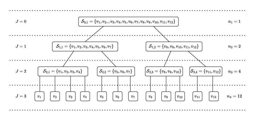
Figure 1: A partition tree $\mathscr{T}_{J}(\mathcal{V})$ for a vertex set $\mathcal{V}$ of 12 vertices and with $J=3$ (4 levels).

In order to construct graph framelet systems analog to the classical wavelet/framelet systems with the multiscale structure, based on a partition tree $\mathscr{T}_{J}({\mathcal{V}})$, we associate each level $j$ with a linear subspace $\mathbb{V}_{j}$ such that $\mathbb{V}_{0}\subsetneq\mathbb{V}_{1}\subsetneq\dots\subsetneq\mathbb{V}_{J}$. Following Mallat’s idea in Multi-resolution analysis (MRA) [42], if we have

$$\mathbb{V}_{j}=\mathbb{V}_{j-1}\oplus\mathbb{W}_{j-1},\quad\mathbb{V}_{j-1}\perp\mathbb{W}_{j-1},\quad j\in[J],$$ (7)

then by doing the decomposition $J-1$ times, we have

$$\mathbb{V}_{J}=\mathbb{V}_{0}\oplus\mathbb{W}_{0}\oplus\mathbb{W}_{1}\oplus\dots\oplus\mathbb{W}_{J-1}$$ (8)

and that $\mathbb{V}_{0},\mathbb{W}_{0},\mathbb{W}_{1},\dots,\mathbb{W}_{J-1}$ are mutually orthogonal. Therefore, to construct a tight frame on $\mathbb{V}_{J}$, it is sufficient to construct tight frames for each $\mathbb{V}_{0},\mathbb{W}_{0},\mathbb{W}_{1},\dots,\mathbb{W}_{J-1}$ and take the union.

The partition tree $\mathscr{T}_{J}({\mathcal{V}})$ suggests that each $\mathbb{V}_{j}$ and $\mathbb{W}_{j}$ should be further decomposed such that

$$\mathbb{V}_{j}:=\oplus_{k=1}^{n_{j}}\mathbb{V}_{j,k},\quad\mathbb{W}_{j}:=\oplus_{k=1}^{n_{j}}\mathbb{W}_{j,k},$$ (9)

where each element in $\mathbb{V}_{j,k}$ or $\mathbb{W}_{j,k}$ is supported on $\mathcal{S}_{j,k}$ and thus $\mathbb{V}_{j,k},k\in[n_{j}]$ (or $\mathbb{W}_{j,k},k\in[n_{j}]$) are mutually orthogonal. Furthermore, the nested structure of $\mathscr{T}_{J}({\mathcal{V}})$ further suggests that

$$\begin{gathered}\oplus_{k^{\prime}\in\mathcal{C}_{j,k}}\mathbb{V}_{j+1,k^{\prime}}=\mathbb{V}_{j,k}\oplus\mathbb{W}_{j,k},\quad\mathbb{V}_{j,k}\perp\mathbb{W}_{j,k}\end{gathered}$$ (10)

for $j\in\{0,\dots,J-1\}$ and $k\in[n_{j}]$.

Assuming that each $\mathbb{V}_{J,k}$ is supported on $\mathcal{S}_{J,k}=\{v_{k}\}$ at the finest level $J$, we can define $\mathbb{V}_{J}:=\mathrm{span}\{\bm{e}_{k}\,|\,k\in[n]\}=\oplus_{k=1}^{n}\mathbb{V}_{J,k}$, where $\mathbb{V}_{J,k}:=\mathrm{span}(\{\bm{e}_{k}\})$ is simply the one-dimensional linear space associated with the vertex $v_{k}$ and generated by the $k$-th canonical basis vector $\bm{e}_{k}:=[0,\ldots,0,1,0\ldots,0]\in\mathbb{R}^{n}$. Note that by the parent-children relation, we can rewrite $\mathbb{V}_{J}$ as

$$\mathbb{V}_{J}=\oplus_{k\in[n_{J-1}]}(\oplus_{k^{\prime}\in\mathcal{C}_{J-1,k}}\mathbb{V}_{J,k^{\prime}}).$$ (11)

It is straightforward to see that (9) and (10) implies (7), which eventually implies (8) since we can decompose $\oplus_{k^{\prime}\in\mathcal{C}_{J-1,k}}\mathbb{V}_{J,k^{\prime}}$ as

$$\oplus_{k^{\prime}\in\mathcal{C}_{J-1,k}}\mathbb{V}_{J,k^{\prime}}=\mathbb{V}_{J-1,k}\oplus\mathbb{W}_{J-1,k}$$ (12)

for each $k\in[n_{J-1}]$, and the procedure can continue from bottom $j=J$ to top $j=0$. Hence, it remains to define a general procedure of decomposition for each non-leaf node in $\mathscr{T}_{J}({\mathcal{V}})$ such that (10) is satisfied. Our next result shows that we indeed can define such a general (bottom-up) procedure and obtain a tight framelet system for $\mathbb{V}_{J}$ based on Cororllary 1 and the partition tree $\mathscr{T}_{J}(\mathcal{V})$.

We first define the $\mathcal{V}$-framelet system based on the partition tree $\mathscr{T}_{J}(\mathcal{V})$.

Definition 2.

Let $\mathscr{T}_{J}({\mathcal{V}})$ be a partition tree as in Definition 1. Let $r_{j}$ be an integer such that $r_{j}\in[\min(|\mathcal{C}_{j,1}|,\dots,|\mathcal{C}_{j,n_{j}})|-1]$ and $\bm{A}^{[j,k]}\in\mathbb{R}^{r_{j}\times|\mathcal{C}_{j,k}|}$ and $\bm{B}^{[j,k]}\in\mathbb{R}^{m_{j,k}\times|\mathcal{C}_{j,k}|}$ be two filter matrices associated with the tree node $p_{j,k}$ for $j=0,\ldots,J-1$ and $k\in[n_{j}]$.

• (Initialization) Define $\mathbb{V}_{J,k}:=\mathrm{span}(\{\bm{e}_{k}\})$ and $\bm{\Phi}^{[J,k]}:=\bm{e}_{k}$ for $k\in[n]$. Let $\mathbb{V}_{J}:=\oplus_{k\in[n]}\mathbb{V}_{J,k}$ and $r_{J}:=1$.

• (Bottom-up Procedure) Recursively define at each level $j$ from $J-1$ to $0$:

  • For each tree node $p_{j,k}$, obtain $\mathbb{V}_{j,k}:=\mathrm{span}(\bm{\Phi}^{[j,k]})$ and $\mathbb{W}_{j,k}=\mathrm{span}(\bm{\Psi}^{[j,k]})$ by Corollary 1 with subspace matrices $\{\bm{X}_{k^{\prime}}:=\bm{\Phi}^{[j+1,k^{\prime}]}\,|\,k^{\prime}\in\mathcal{C}_{j,k}\}$ and the two filter matrices $\bm{A}^{[j,k]}$ and $\bm{B}^{[j,k]}$. More precisely, let $\bm{X}:=\llbracket\bm{X}_{k^{\prime}}\rrbracket_{k^{\prime}\in\mathcal{C}_{j,k}}$. Then we have

    $$\bm{\Phi}^{[j,k]}=\mathcal{A}^{[j,k]}\bm{X},\quad\bm{\Psi}^{[j,k]}=\mathcal{B}^{[j,k]}\bm{X},$$ (13)

    where $\mathcal{A}^{[j,k]},\mathcal{B}^{[j,k]}$ are matrices corresponding to (6) in Corollary 1.

  • Define $\mathbb{V}_{j}:=\mathrm{span}(\bm{\Phi}_{j})$ with $\bm{\Phi}_{j}:=\llbracket\bm{\Phi}^{[j,k]}\rrbracket_{k\in[n_{j}]}$ and $\mathbb{W}_{j}:=\mathrm{span}(\bm{\Psi}_{j})$ with $\bm{\Psi}_{j}:=\llbracket\bm{\Psi}^{[j,k]}\rrbracket_{k\in[n_{j}]}$.

• (Finalization) For each $J_{0}=0,\ldots,J$, define the $\mathcal{V}$-framelet system associate with the partition tree $\mathscr{T}_{J}(\mathcal{V})$ and determined by the filter matrices as

  $$\mathcal{F}_{J_{0}}^{J}(\mathcal{V}):= \mathcal{F}_{J_{0}}(\{(\bm{A}^{[j,k]},\bm{B}^{[j,k]})\,|\,k\in[n_{j}]\}_{j=J_{0}}^{J-1})$$ (14)

  $$:= \bm{\Phi}_{J_{0}}\cup\bm{\Psi}_{J_{0}}\cup\cdots\cup\bm{\Psi}_{J-1}.$$

Now we are ready to state the main theorem for the construction of a general tight $\mathcal{V}$-framelet system for $\mathbb{V}_{J}$.

Theorem 1.

Adopt the notations in Definition 2. Assume that the filter matrices $\bm{A}^{[j,k]}$ and $\bm{B}^{[j,k]}$ satisfy

$$\bm{A}^{[j,k]}({\bm{A}^{[j,k]}})^{\top} =\bm{I},$$ (15)

$$\bm{B}^{[j,k]}({\bm{A}^{[j,k]}})^{\top} =\bm{0},$$ (16)

$$({\bm{B}^{[j,k]}})^{\top}\bm{B}^{[j,k]} =\bm{I}-({\bm{A}^{[j,k]}})^{\top}\bm{A}^{[j,k]},$$ (17)

for $j\in\{0,\dots,J-1\}$ and $k\in[n_{j}]$. Then the following statements hold.

• $\mathbb{V}_{j}=\oplus_{k=1}^{n_{j}}\mathbb{V}_{j,k}$, $\mathbb{W}_{j}=\oplus_{k=1}^{n_{j}}\mathbb{W}_{j,k}$ for $j=0,\ldots,J-1$, and $\mathbb{V}_{j}=\mathbb{V}_{j-1}\oplus\mathbb{W}_{j-1},\mathbb{V}_{j-1}\perp\mathbb{W}_{j-1}$ for $j\in[J]$.

• $\mathbb{V}_{J}=\mathbb{V}_{j}\oplus\mathbb{W}_{j}\oplus\mathbb{W}_{j+1}\oplus\dots\oplus\mathbb{W}_{J-1}$ for $j=0,\ldots,J-1$. In particular, $\mathbb{V}_{J}=\mathbb{V}_{0}\oplus\mathbb{W}_{0}\oplus\mathbb{W}_{1}\oplus\dots\oplus\mathbb{W}_{J-1}$.

• $\mathcal{F}_{J_{0}}^{J}(\mathcal{V})$ is a tight frame for $\mathbb{V}_{J}$ for all $J_{0}=0,\ldots,J-1$.

Proof.

We apply mathematical induction on $j$ (decreasingly) to prove that for each $j\in{0,\dots,J-1}$, all the subspaces $\mathbb{V}_{j+1,k^{\prime}}=\mathrm{span}(\bm{\Phi}^{[j+1,k^{\prime}]})$ in the previous level have the same dimension and conditions in Corrolary 1 are satisfied with $\bm{X}_{k}^{\prime}:=\bm{\Phi}^{[j+1,k^{\prime}]},k^{\prime}\in\mathcal{C}_{j,k}$. Hence, by the results of Corollary 1, we can obtain the conclusions of items (i)–(iii) of the theorem.

• Base case: By definition, each $\mathbb{V}_{J,k},k\in[n]$ is spaned by $\bm{\Phi}^{[j+1,k]}=\bm{e}_{k}\in\mathbb{R}^{r_{J}\times n}$, which is $r_{J}$-dimensional ($r_{J}=1$). Note that $\mathbb{V}_{J}=\oplus_{k\in[n_{J-1}]}\oplus_{k^{\prime}\in\mathcal{C}_{J-1,k}}\mathbb{V}_{J,k^{\prime}}$.

• Induction hypothesis: Assume that at level $j+1$ with $0\leq j\leq J-1$, each $\mathbb{V}_{j+1,k}=\mathrm{span}(\bm{\Phi}^{[j+1,k]})$ has the same dimension $R_{j+1}:=\prod_{i=j+1}^{J}r_{i}$ for all $k\in[n_{j+1}]$, where each $\bm{\Phi}^{[j+1,k]}$ is formed by othonormal row vectors supported on $\mathcal{S}_{j+1,k}$.

• Induction step: We next prove that each $\mathbb{V}_{j,k}=\mathrm{span}(\bm{\Phi}^{[j,k]})$ also has the same dimension $R_{j}:=\prod_{i=j}^{J}r_{i}$ for all $k\in[n_{j}]$ with each $\bm{\Phi}^{[j,k]}$ being formed by othonormal row vectors. In fact, fixed the node $p_{j,k}$, it has its children nodes $p_{j+1,k^{\prime}},k^{\prime}\in\mathcal{C}_{j,k}$. Consider $\bm{X}_{k^{\prime}}:=\bm{\Phi}^{[j+1,k^{\prime}]}\in\mathbb{R}^{R_{j+1}\times n}$, $k^{\prime}\in\mathcal{C}_{j,k}$. By (15) – (17), the conditions of Corollary 1 are satisfied with these subspace matrices $\bm{X}_{k^{\prime}}$ and the two filter matrices $\bm{A}^{[j,k]},\bm{B}^{[j,k]}$. Thus its conclusions can be obtained. That is, $\mathbb{V}_{\bm{X}}:=\oplus_{k^{\prime}\in\mathcal{C}_{j,k}}\mathbb{V}_{j+1,k^{\prime}}=\mathbb{V}_{j,k}\oplus\mathbb{W}_{j,k},\mathbb{V}_{j,k}\perp\mathbb{W}_{j,k}$, and the rows of $\bm{\Phi}^{[j,k]}$ form an orthonormal basis for $\mathbb{V}_{j,k}$. Moreover, the rows of $\bm{\Psi}^{[j,k]}$ form a tight frame for $\mathbb{W}_{j,k}$. Note that the dimension of $\mathbb{V}_{j,k}$ satisfies $\mathrm{dim}(\mathbb{V}_{j,k})\equiv r_{j}R_{j+1}=\prod_{i=j}^{J}r_{i}$ for all $k\in[n_{j}]$.

• Conclusion: Therefore, for each $j=0,\ldots,J$, the space $\mathbb{V}_{j,k}=\mathrm{span}(\bm{\Phi}^{[j,k]})$ has the same dimension $R_{j}$ for all $k\in[n_{j}]$ with each $\bm{\Phi}^{[j,k]}$ being formed by orthonormal row vectors.

Consequently, item (i) holds and it implies item (ii). Item (iii) follows from item (ii) and the result that the rows of $\bm{\Psi}^{[j,k]}$ form a tight frame for $\mathbb{W}_{j,k}$. ∎

The construction of $\mathcal{V}$-framelet system in Theorem 1 is formulated in Algorithm 2. Before we proceed, we have the following remarks.

Algorithm 2 Generation of the $\mathcal{V}$-Framelet System

1:Input: A partition tree $\mathscr{T}_{J}({\mathcal{V}})$, a set of postive integers $\{r_{j}\}_{j=1}^{J}$, matrices $\bm{A}^{[j,k]}\in\mathbb{R}^{r_{j}\times|\mathcal{C}_{j,k}|},\bm{B}^{[j,k]}\in\mathbb{R}^{m_{j,k}\times|\mathcal{C}_{j,k}|},k\in[n_{j}],j\in\{0,\dots,J-1\}$.

2:$\bm{\Phi}^{[J,k]}:=\bm{e}_{k},k\in[n]$.

3:for $j=J-1$ to $0$ do

4:     for $k=1$ to $n_{j}$ do

5:         $\bm{\Xi}_{\ell}:=\text{{CONCAT}}(\{\bm{\Phi}^{[j+1,k^{\prime}]}_{\ell,:}\}_{k^{\prime}\in\mathcal{C}_{j,k}}),\,\ell\in[r_{j}]$.

6:         $\bm{\Phi}^{[j,k]}:=\text{{CONCAT}}(\{\bm{A}^{[j,k]}\bm{\Xi}_{\ell}\}_{\ell=1}^{r_{j}})$.

7:         $\bm{\Psi}^{[j,k]}:=\text{{CONCAT}}(\{\bm{B}^{[j,k]}\bm{\Xi}_{\ell}\}_{\ell=1}^{r_{j}})$.      

8:     $\bm{\Phi}_{j}:=\cup_{k=1}^{n_{j}}\bm{\Phi}^{[j,k]},\quad\bm{\Psi}_{j}:=\cup_{k=1}^{n_{j}}\bm{\Psi}^{[j,k]}$.

9:Output: $\{\bm{\Phi}_{0}\}\cup\{\bm{\Psi}_{j}\}_{j=0}^{J-1}$.

Remark 2.

Note that the construction of $\mathcal{V}$-framelet systems only involves the vertex set $\mathcal{V}$ and the partition tree $\mathscr{T}_{J}(\mathcal{V})$. No graph structure, such as the edge set $\mathcal{E}$ or the adjacency matrix, is involved. Such construction based on the hierarchical partitions of a vertex set has the benefit of providing a mathematical generality. We discuss the graph framelet systems in the next subsection that utilize both the vertex set $\mathcal{V}$ and the edge set $\mathcal{E}$.

Remark 3.

As in classical wavelet/framelet theory, we called the elements of $\bm{\Phi}_{j}$ scaling functions and the elements of $\bm{\Psi}_{j}$ framelets. The framelets have localized supports, i.e. framelets in $\mathbb{W}_{j,k}$ are supported on $\mathcal{S}_{j,k}$.

Remark 4.

The dimension of $\mathbb{V}_{j}$ is $R_{j}=\Pi_{i=j}^{J}r_{i}$, which can be controlled by varying the $r_{i}$. As mentioned in the introduction, the orthogonality to $\mathbb{V}_{j}$ can be used to define vanishing moments of the framelet system. Note that the $\mathcal{V}$-framelet system $\mathcal{F}_{J_{0}}^{J}(\mathcal{V})$ as defined in (14) has its framelets all from $\mathbb{W}_{j}$ for $j\geq J_{0}$ and hence all orthogonal to $\mathbb{V}_{J_{0}}$. We call the such a framelet system $\mathcal{F}_{J_{0}}^{J}(\mathcal{V})$ has generalized $R_{J_{0}}$ vanishing moments.

Remark 5.

The condition in (17) can be considered as a generalized version of the unitary extension principle in classic wavelet/framelet theories [43], which requires the filter bank to form a partition of unity. By analogy, we can regard $\bm{A}^{[j,k]},\bm{B}^{[j,k]}$ as filters and their union as a filter bank.

Remark 6.

In [28], Haar-type tight framelet system is obtained by defining $\bm{A}^{[j,k]}:=\frac{1}{\sqrt{|\mathcal{C}_{j,k}|}}\begin{bmatrix}1,\dots,1\end{bmatrix}\in\mathbb{R}^{1\times|\mathcal{C}_{j,k}|}$ and $\bm{B}^{[j,k]}\in\mathbb{R}^{\frac{|\mathcal{C}_{j,k}|(|\mathcal{C}_{j,k}|-1)}{2}\times|\mathcal{C}_{j,k}|}$ whose rows $\bm{B}^{[j,k]}_{m,:}:=\bm{b}^{m}$, $1\leq m\leq\frac{|\mathcal{C}_{j,k}|(|\mathcal{C}_{j,k}|-1)}{2}$, are given by $\bm{b}^{m}\in\mathbb{R}^{1\times|\mathcal{C}_{j,k}|}$ with its $i$th entry being defined by

$$\bm{b}^{m}_{i}:=\left\{\begin{aligned} \frac{1}{{|\mathcal{C}_{j,k}|}}\quad&i=s,\\ \frac{-1}{\sqrt{|\mathcal{C}_{j,k}|}}\quad&i=t,\\ 0\quad&\text{otherwise,}\end{aligned}\right.$$

where $m$ is uniquely determined by the integers $s,t$ with $1\leq s<t\leq|\mathcal{C}_{j,k}|$ as $m:=m(s,t,|\mathcal{C}_{j,k}|):=\frac{(2|\mathcal{C}_{j,k}|-s)(s-1)}{2}+s-t$. It is shown that (17) in Theorem 1 is satisfied. In summary, the rows of $\bm{B}^{[j,k]}$ is constructed by enumerating pairs of indices in $\mathcal{C}_{j,k}$ and assigning the same constant with different signs, which resemble classic Haar wavelets/filters. Our general construction includes [28] as a special case.

II-C Construction of $\mathcal{G}$-Framelet Systems

As we point out in Remark 2, the $\mathcal{V}$-framelet systems do not involve the other graph structure such as the edge set $\mathcal{E}$. However, they do depend on the partition tree $\mathscr{T}_{J}(\mathcal{V})$ and how to obtain such a partition tree is closely related to the graph $\mathcal{G}=(\mathcal{V},\mathcal{E},\bm{W})$. We next discuss how we can obtain the partition tree from a given graph $\mathcal{G}$ and define the so-called graph-involved $\mathcal{G}$-framelet systems.

We first discuss the realization of the nested structure of a partition tree. It is known that edges in graphs intuitively represent a notion of proximity among nodes. Thus, to represent scales (levels) on graphs analog to the Euclidean domains, a common practice is to apply a series of clustering (coarsing) on graphs. In detail, given $\mathcal{G}=(\mathcal{V},\mathcal{E},\bm{W})$ with $\mathcal{V}:=\{v_{1},\ldots,v_{n}\}$, the clusters on $\mathcal{V}$ are formed through certain algorithms, e.g., $K$-means clustering, based on $\mathcal{E}$ such that connected nodes are more likely to be in the same clusters. Assuming that the clustering algorithm on $\mathcal{G}$ resulted in $n^{\prime}$ clusters, denoted as $\mathcal{V}^{\prime}=\{v_{1}^{\prime},\ldots,v_{n^{\prime}}^{\prime}\}$, where each $v_{i}^{\prime}=\{v_{i_{1}},\ldots,v_{i_{n_{i}}}\}\subseteq\mathcal{V}$, $v_{i}^{\prime}\cap v_{j}^{\prime}=\varnothing$ for $i\neq j$, and $\cup_{i=1}^{n^{\prime}}v_{i}^{\prime}=\mathcal{V}$. Then a graph $\mathcal{G}^{\prime}:=(\mathcal{V}^{\prime},\mathcal{E}^{\prime},\bm{W}^{\prime})$ can be formed from these clusters through the definition of its adjacency matrix $\bm{W}^{\prime}=(w_{ij}^{\prime})_{1\leq i,j\leq n^{\prime}}$ as

$$w_{ij}^{\prime}:=\sum_{p\in v_{i}^{\prime}}\sum_{q\in v_{j}^{\prime}}w_{pq},\quad i,j=1,\ldots,n^{\prime},$$

where $w_{ij}^{\prime}$ is the weight between $v_{i}^{\prime},v_{j}^{\prime}\in\mathcal{V}^{\prime}$ while $w_{pq}$ is the original weight between vertices $p,q\in\mathcal{V}$.

In summary, the nodes of $\mathcal{G}^{\prime}$ represent clusters and the edge weight on $\mathcal{G}^{\prime}$ is determine by summing of the edge weight among nodes of two clusters. We called $\mathcal{G}^{\prime}$ a coarse-grained graph of $\mathcal{G}$ [44]. Based on the coarse-grained graph, we can give the definition of multi-graph partition trees.

Definition 3.

A multi-graph partition tree $\mathscr{T}_{J}({\mathcal{G}})$ of $\mathcal{G}=(\mathcal{V},\mathcal{E},\bm{W})$ with $J+1,J\in\mathbb{N}$ levels is a partition tree $\mathscr{T}_{J}({\mathcal{V}})$ as defined in Definition 1 such that each $j\in\{0,\dots,J\}$ is associated with a coarse-grained graph $\mathcal{G}^{j}=(\mathcal{V}^{j},\mathcal{E}^{j})$ of $\mathcal{G}$ and $\mathcal{V}^{j}=\{\mathcal{S}_{j,k}\,|\,k\in[n_{j}]\}$. In particular, $\mathcal{G}^{J}\equiv\mathcal{G}$, where we consider a vertex in $\mathcal{G}^{J}$ as a cluster of singleton.

An intuitive and equivalent interpretation of the definition above is that a multi-graph partition tree is a partition tree by generated successively forming coarsed-grained graphs $\mathcal{G}^{J-1},\mathcal{G}^{J-1}\dots,\mathcal{G}^{0}$ such that $\mathcal{G}^{j}$ is a coarse-grained graph of $\mathcal{G}^{j+1},j\in[J-1]$. Since $\mathscr{T}_{J}(\mathcal{G})$ is associated with a partition tree $\mathscr{T}_{J}(\mathcal{V})$, we can construct $\mathcal{V}$-framelet systems as in Definition 2. We have the following definition.

Definition 4.

Let $\mathscr{T}_{J}(\mathcal{G})$ be a multi-graph partition tree associated with a graph $\mathcal{G}=(\mathcal{V},\mathcal{E},\bm{W})$. Let {$r_{j}$, $\bm{A}^{[j,k]}$, $\bm{B}^{[j,k]}\,|\,j=0,\ldots,J-1;k\in[n_{j}]\}$ be the set of integers and filter matrices satisfying the assumptions of Theorem 1. Then for $J_{0}=0,\ldots,J-1$, the $\mathcal{V}$-framelet system $\mathcal{F}_{J_{0}}^{J}(\mathcal{V})$ as in (14) is a tight frame for $\mathbb{V}_{J}=\mathrm{span}\{\bm{e}_{k}\,|\,k\in[n]\}=L_{2}(\mathcal{G})$, which we call a (graph-involved) $\mathcal{G}$-framelet (GIF) system. In such a case, we simply denote $\mathcal{F}_{J_{0}}^{J}(\mathcal{G}):=\mathcal{F}_{J_{0}}^{J}(\mathcal{V})$ to indicate the role played by $\mathcal{G}$. In particular, we define for the special case $J_{0}=0$, the GIF system $\mathcal{F}_{0}^{J}(\mathcal{G})$ as

$$\mathsf{GIF}_{J}(\mathcal{G}):=\mathcal{F}_{0}^{J}(\mathcal{G})=\bm{\Phi}_{0}\oplus\bm{\Psi}_{0}\oplus\cdots\oplus\bm{\Psi}_{J-1}.$$ (18)

Remark 7.

When $r_{j}=1$ for all $j=\{0,\dots,J-1\}$, the filter matrix $\bm{A}^{[j,k]}$ consists of the first eigenvector of $\bm{L}^{[j,k]}$, and the rows of $\bm{B}^{[j,k]}$ are the remaining eigenvectors of $\bm{L}^{[j,k]}$, where $\bm{L}^{[j,k]}$ is the graph Laplacian matrix of the subgraph of $\mathcal{G}^{j+1}$ induced by the nodes $\{\mathcal{S}_{j+1,k^{\prime}}\,|\,k^{\prime}\in\mathcal{C}_{j,k}\}$, then the $\mathcal{G}$-framelet system $\mathsf{GIF}_{J}(\mathcal{G})$ is an orthonormal basis, which corresponds to the case $p=2$ in [12].

III Graph Framelet Transforms

In this section, we focus on the fast transform algorithms based on the $\mathcal{G}$-framelet systems as well as their computational complexity.

III-A Graph Framelet Transforms

Similar to the discrete wavelet/framelet transforms, the iterative nature of the tight graph framelet systems $\mathcal{F}_{J_{0}}^{J}(\mathcal{G})$ for $J_{0}=0,\ldots,J-1$ can be used to derive the graph framelet transforms for graph signals $\bm{f}\in L_{2}(\mathcal{G})$. In fact, given such an $\bm{f}$, which is a row vector of size $n$, by the tightness of the system $\mathcal{F}_{J_{0}}^{J}(\mathcal{G})$, it holds for $J_{0}=0,\ldots,J-1$ that

$$\bm{f}=\sum_{k\in[n_{J_{0}}]}\bm{c}^{[J_{0},k]}\bm{\Phi}^{[J_{0},k]}+\sum_{j=J_{0}}^{J-1}\sum_{k\in[n_{j}]}\bm{d}^{[j,k]}\bm{\Psi}^{[j,k]},$$ (19)

where

$$\bm{c}^{[j,k]}:=\langle\bm{f},\bm{\Phi}^{[j,k]}\rangle,\quad\bm{d}^{[j,k]}:=\langle\bm{f},\bm{\Psi}^{[j,k]}\rangle,$$ (20)

and the inner product is defined by

$$\langle\bm{A},\bm{B}\rangle:=\bm{A}\bm{B}^{\top},\quad\bm{A}\in\mathbb{R}^{r\times m},\bm{B}\in\mathbb{R}^{s\times m}.$$

The graph framelet transforms consists of the analysis and the synthesis phases, where the analysis step is to decompose a given signal $\bm{f}$ into its framelet coefficient sequences: $\bm{c}^{[J_{0},k]},\bm{d}^{[j,k]}$, $j=J_{0},\ldots,J-1,k\in[n_{j}]$, and the synthesis step is to reconstruct a signal $\bm{f}$ from such a given framelet coefficient sequences. Recall that $\llbracket\cdot\rrbracket$ and $\bm{\llparenthesis}\cdot\bm{\rrparenthesis}$ are row-wise and column-wise concatenation, respectively. The following result discusses the one-level decomposition and reconstruction of the graph framelet transforms.

Corollary 2.

Let $\bm{f}\in L_{2}(\mathcal{G})$ be a graph signal and $\bm{c}^{[j,k]},\bm{d}^{[j,k]}$ denote the vector coefficients with respect to $\bm{\Phi}^{[j,k]},\bm{\Psi}^{[j,k]}$ as defined in (20) from the tight graph framelet system $\mathsf{GIF}_{J}(\mathcal{G})$. Then

$$\left\{\begin{matrix}\bm{c}^{[j,k]}&=\langle\bm{\llparenthesis}\bm{c}^{[j+1,k^{\prime}]}\bm{\rrparenthesis}_{k^{\prime}\in\mathcal{C}_{j,k}},\mathcal{A}^{[j,k]}\rangle,\\ \\ \bm{d}^{[j,k]}&=\langle\bm{\llparenthesis}\bm{c}^{[j+1,k^{\prime}]}\bm{\rrparenthesis}_{k^{\prime}\in\mathcal{C}_{j,k}},\mathcal{B}^{[j,k]}\rangle,\\ \end{matrix}\right.$$ (21)

and

$$(\bm{c}^{[j+1,k^{\prime}]})_{k^{\prime}\in\mathcal{C}_{j,k}}=\bm{c}^{[j,k]}\mathcal{A}^{[j,k]}+\bm{d}^{[j,k]}\mathcal{B}^{[j,k]},\\$$ (22)

where $\mathcal{A}^{[j,k]},\mathcal{B}^{[j,k]}$ are those matrices as in (13) satisfying $(\mathcal{A}^{[j,k]})^{\top}\mathcal{A}^{[j,k]}+(\mathcal{B}^{[j,k]})^{\top}\mathcal{B}^{[j,k]}=\bm{I}$.

Proof.

Note that

$$\bm{c}^{[j,k]} =\langle\bm{f},\bm{\Phi}^{[j,k]}\rangle=\langle\bm{f},\mathcal{A}^{[j,k]}\llbracket\bm{\Phi}^{[j+1,k^{\prime}]}\rrbracket_{k^{\prime}\in\mathcal{C}_{j,k}}\rangle$$

$$=\bm{f}\llbracket\bm{\Phi}^{[j+1,k^{\prime}]}\rrbracket_{k^{\prime}\in\mathcal{C}_{j,k}}^{\top}(\mathcal{A}^{[j,k]})^{\top}$$

$$=\bm{\llparenthesis}\langle\bm{f},\bm{\Phi}^{[j+1,k^{\prime}]}\rangle\bm{\rrparenthesis}_{k^{\prime}\in\mathcal{C}_{j,k}}(\mathcal{A}^{[j,k]})^{\top}$$

$$=\bm{\llparenthesis}\bm{c}^{[j+1,k^{\prime}]}\bm{\rrparenthesis}_{k^{\prime}\in\mathcal{C}_{j,k}}(\mathcal{A}^{[j,k]})^{\top}$$

$$=\langle\bm{\llparenthesis}\bm{c}^{[j+1,k^{\prime}]}\bm{\rrparenthesis}_{k^{\prime}\in\mathcal{C}_{j,k}},\mathcal{A}^{[j,k]}\rangle,$$

and similarly, we have

$$\bm{d}^{[j,k]} =\langle\bm{f},\bm{\Psi}^{[j,k]}\rangle=\bm{\llparenthesis}\bm{c}^{[j+1,k^{\prime}]}\bm{\rrparenthesis}_{k^{\prime}\in\mathcal{C}_{j,k}}(\mathcal{B}^{[j,k]})^{\top}$$

$$=\langle\bm{\llparenthesis}\bm{c}^{[j+1,k^{\prime}]}\bm{\rrparenthesis}_{k^{\prime}\in\mathcal{C}_{j,k}},\mathcal{B}^{[j,k]}\rangle.$$

On the other hand, in view of the condition $(\mathcal{A}^{[j,k]})^{\top}\mathcal{A}^{[j,k]}+(\mathcal{B}^{[j,k]})^{\top}\mathcal{B}^{[j,k]}=\bm{I}$, together with (21), it is easy to see that (22) holds. ∎

The one-level decomposition and reconstruction relations in Corollary 2 can be applied successively to decompose or reconstruct a graph signal $\bm{f}$. Such multi-level decomposition (forward transform) and reconstruction (backward transform) procedures are summarized in Algorithms 3 and 4, and illustrated in Figures 2 and 3, respectively. Here, in Algorithm 4, the notion $\text{ID}(k^{\prime})$ is defined by sorting $k^{\prime}\in\mathcal{C}_{j,k}$ increasingly to index each $k^{\prime}\in\mathcal{C}_{j,k}$ by a unique integer $\text{ID}(k^{\prime})$ in $\{1,\dots,|\mathcal{C}_{j,k}|\}$ such that $\text{ID}(k^{\prime})<\text{ID}(k^{\prime\prime})\Leftrightarrow k^{\prime}\leq k^{\prime\prime}$.

Algorithm 3 FORWARD $\mathsf{GIF}$-TRANSFORM

1:Input: A signal $\bm{f}=[f_{1},\ldots,f_{n}]\in L^{2}(\mathcal{G})$ and filter matrices $\bm{A}^{[j,k]}\in\mathbb{R}^{r_{j}\times|\mathcal{C}_{j,k}|},\bm{B}^{[j,k]}\in\mathbb{R}^{m_{j,k}\times|\mathcal{C}_{j,k}|},k\in[n_{j}],j\in\{0,\dots,J-1\}$ associated with a multi-graph tree partition $\mathscr{F}_{J}(\mathcal{G})$.

2:$\bm{c}^{[J,k]}:={f}_{k},k\in[n]$.

3:for $j=J-1$ to $0$ do

4:     for $k=1$ to $n_{j}$ do

5:         $\bm{c}^{[j,k]}:=\text{{VEC}}(\bm{A}^{[j,k]}\text{{CONCAT}}(\{\bm{c}^{[j+1,k^{\prime}]}\}_{k^{\prime}\in\mathcal{C}_{j,k}}))$

6:         $\bm{d}^{[j,k]}:=\text{{VEC}}(\bm{B}^{[j,k]}\text{{CONCAT}}(\{\bm{c}^{[j+1,k^{\prime}]}\}_{k^{\prime}\in\mathcal{C}_{j,k}}))$      

7:Output: $\{\bm{c}^{[0,1]}\}\cup\{\bm{d}^{[j,k]}\,|\,k\in[n_{j}]\}_{j=0}^{J-1}$

Algorithm 4 BACKWARD $\mathsf{GIF}$-TRANSFORM

1:Input: Coefficient vectors $\{\bm{c}^{[0,1]}\}\cup\{\bm{d}^{[j,k]}\,|\,k\in[n_{j}]\}_{j=0}^{J-1}$ and filter matrices $\bm{A}^{[j,k]}\in\mathbb{R}^{r_{j}\times|\mathcal{C}_{j,k}|},\bm{B}^{[j,k]}\in\mathbb{R}^{m_{j,k}\times|\mathcal{C}_{j,k}|},k\in[n_{j}],j\in\{0,\dots,J-1\}$.

2:for $j=0$ to $J-1$ do

3:     for $k=1$ to $n_{j}$ do

4:         $\bm{X}:={\bm{A}^{[j,k]}}^{\top}\text{{MAT}}(\bm{c}^{[j,k]},r_{j})+{\bm{B}^{[j,k]}}^{\top}\text{{MAT}}(\bm{d}^{[j,k]}\allowbreak,m_{j,k})$

5:         for $k^{\prime}\in\mathcal{C}_{j,k}$ do

6:              $\bm{c}^{[j+1,k^{\prime}]}:=\bm{X}_{\text{{ID}}(k^{\prime}),:}$               

7:Output: $\{\bm{c}^{[J,k]}\}_{k=1}^{n}$

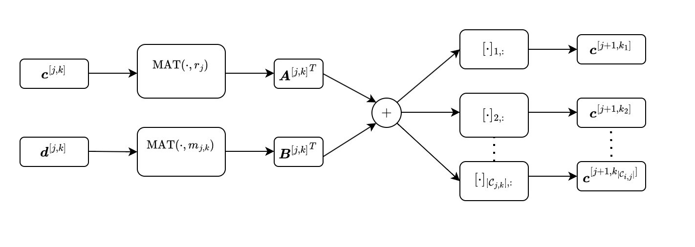
Figure 2: An illustration of computing coefficient vectors on a non-leaf node of $\mathscr{T}_{J}(\mathcal{G})$. The whole transform is computed iteratively in a bottom-up manner at each non-leaf node of $\mathscr{T}_{J}(\mathcal{G})$

.

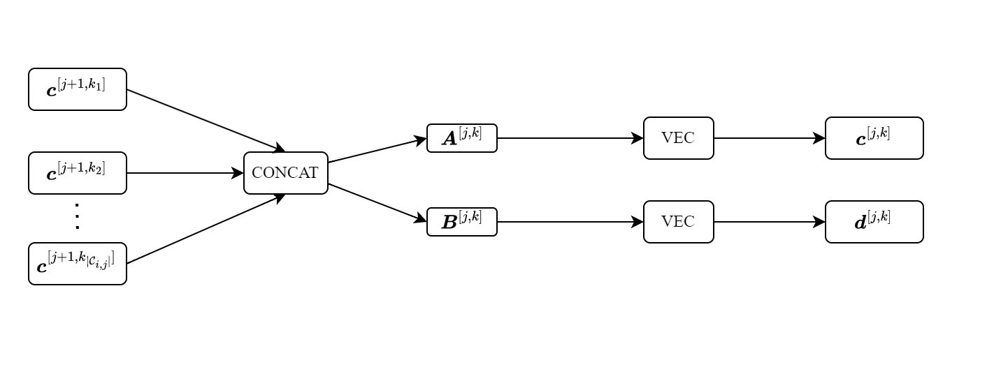
Figure 3: An illustration of reconstruction on a non-leaf node of $\mathscr{T}_{J}(\mathcal{G})$. The whole transform is computed iteratively in a top-down manner at each non-leaf node of $\mathscr{T}_{J}(\mathcal{G})$. Here, $[\cdot]_{i,:}$ denotes the operation of extracting the $i$-th row of the matrix.

III-B Computational Complexity

we next discuss the computational complexity of Algorithms 3 and 4. We have the following theorem.

Theorem 2.

Adopt the notations in Theorem 1 and Corollary 2. Assume that the computational complexity of CONCAT, VEC, and MAT are of order $\mathcal{O}(\text{size of input})$, and there exist positive constants $t,s,r,\alpha,m$ such that $\min\{t,s,r,\alpha,m\}\geq 1$ and

$$t\leq|\mathcal{C}_{j,k}|\leq s,\,s\leq t^{\alpha},\,r_{j}\leq r\leq\frac{s}{2},\,m_{j,k}\leq m$$ (23)

for all $k\in[n_{j}]$ and all $j\in\{0,\dots,J-1\}$. Then the computational complexity of Algorithm 3 or 4 is of order $\mathcal{O}((r+m)\cdot n^{\alpha})$

Proof.

By the tree structure of $\mathscr{T}_{J}(\mathcal{V})$, we can deduce that

$$J\leq\log_{t}(n),\,t^{j}\leq n_{j}\leq s^{j},R_{j}\leq r^{J-j},\,j\in\{0,\dots,J\}.$$

For a fixed level $j$, the computational complexity at line 5 of Algorithm 3 is of order

$$\mathcal{O}(s\cdot r^{J-j-1}) (\text{{CONCAT}}),$$

$$+ \mathcal{O}(s\cdot r^{J-j}) (\text{{Matrix multiplication with }}\bm{A}^{[j,k]}),$$

$$+ \mathcal{O}(r^{J-j}) (\text{{VEC}}).$$

Therefore, if excluding line 6, the total computational complexity is of order

$$\mathcal{O}\Big{(}\sum^{J-1}_{j=0}s^{j}r^{J-j}\left(sr^{-1}+s+1\right)\Big{)}=\mathcal{O}\Big{(}\sum^{J-1}_{j=0}s^{j}r^{J-j}S_{1}\Big{)}$$

where $S_{1}:=sr^{-1}+s+1=s(r^{-1}+1+s^{-1})\leq 3s$. By (23) and the identity $\sum_{j=0}^{J-1}x^{j}=\frac{x^{J}-1}{x-1}$, we have $\sum_{j=0}^{J}s^{j}r^{J-j}=r^{J}\frac{(s/r)^{J}-1}{s/r-1}\leq r^{J}\frac{(s/r)^{J}}{s/r-s/(2r)}\leq 2rs^{J-1}$ and the order of computational complexity becomes $\mathcal{O}(r\cdot s^{J-1}\cdot S_{1})$, which is essentially of order $\mathcal{O}(r\cdot n^{\alpha})$ in view of $s\leq t^{\alpha}$ and $J\leq\log_{t}(n)$.

Similarly, at line 6 of Algorithm 3, if line 5 is excluded, the total computational complexity is of order

$$\mathcal{O}\Big{(}\sum^{J-1}_{j=0}s^{j}r^{J-j}\left(sr^{-1}+smr^{-1}+mr^{-1}\right)\Big{)}=\mathcal{O}(rs^{J-1}\cdot S_{2}),$$

where $S_{2}:=sr^{-1}+smr^{-1}+mr^{-1}\leq 3smr^{-1}$, which is essentially of order $\mathcal{O}\left(m\cdot n^{\alpha}\right)$

Combine the two terms we have order $\mathcal{O}\left((r+m)\cdot n^{\alpha}\right)$ of computational complexity for Algorithm 3.

As for Algorithm 4, it is obvious that lines 4, 5, and 6 together become the reverse of lines 5 and 6 of Algorithm 3, and that the amounts of computation are the same. Thus, the computational complexity of Algorithm 4 is the same as that of Algorithm 3. ∎

Remark 8.

The number $\alpha$ indicates the balance of children-node sizes $|\mathcal{C}_{j,k}|$. If $\mathscr{T}_{J}(\mathcal{V})$ is a $K$-tree, i.e. each tree node has exactly $K$ children, then $\alpha=1$ and we have order $\mathcal{O}((r+m)n)$ of computational complexity. By definition, $m$ is an upper-bound of the numbers of rows of each $\bm{B}^{[j,k]}$. When the rows of $\bm{B}^{[j,k]}$ form a basis of $\mathrm{span}{(\bm{B}^{[j,k]})}$, it is obvious that it is bounded above $|\mathcal{C}_{j,k}|$ and further bounded by $s$. Thus, $m$ can be $s$. When the rows of $\bm{B}^{[j,k]}$ form a frame of $\mathrm{span}{(\bm{B}^{[j,k]})}$, we can control the number of elements of the frame to be a multiple of the dimension of $\mathrm{span}{(\bm{B}^{[j,k]})}$ and thus $m$ can be a multiple of $s$. In both cases, we have $r+m=O(s)$ and the complexity further becomes $O(s\cdot n)$. In summary, constructing a partition tree with balanced and small children-node sizes ensures a low computation complexity. This is compatible with the complexity analysis in [28].

IV Data-adpative Graph Framelet Systems

Given a multi-graph partition tree, we still need to specify the filter matrices $\bm{A}^{[j,k]},\bm{B}^{[j,k]}$ to obtain a graph-involved framelet system $\mathsf{GIF}_{J}(\mathcal{G})$. In this section, we focus on learning such filter matrices from a certain family of signals through optimization techniques on Stiefel manifolds. For convienience, we call $\bm{A}^{[j,k]}$ and $\bm{B}^{[j,k]}$ associating with $\mathbb{V}_{j,k},\mathbb{W}_{j,k}$ the low-pass filter and high-pass filter, respectively.

Suppose we are given $n_{f}$ sample graph signals $\bm{f}_{1}$, $\bm{f}_{2}$, $\dots$, $\bm{f}_{n_{f}}$ of a family $\mathfrak{F}$ with low-dimensional structure, i.e., the family $\mathfrak{F}$ is approximately contained in a low-dimensional linear space in $\mathbb{R}^{n}$. Similar to the setting in machine learning tasks, we specify the parameters (filters) by learning from these samples and expect that the learned $\mathsf{GIF}_{J}(\mathcal{G})$ will be able to provide sparse representation for any signal in $\mathfrak{F}$.

For determining the low-pass filters, we aim at learning low-pass filters so that the space $\mathbb{V}_{0}=\mathrm{span}(\bm{\Phi}_{0})$ provides the best fitting of the samples in the $l^{2}$ sense. That is, for any signal $\bm{f}\in\mathfrak{F}$, most of the energy of $\bm{f}$ is contained in its projection on $\mathbb{V}_{0}$. In such a way, we could capture the low-dimensional structure of the family $\mathfrak{F}$. Once we obtained the low-pass filters, in view of the generalized vanishing moments, i.e., orthogonality between $\mathbb{V}_{0}$ and $\mathbb{W}_{j}$, most of the coefficients in $\mathbb{W}_{j}$ are expected to be small or even zero. Therefore, in such a case, the $\mathcal{G}$-framelet system $\mathsf{GIF}_{J}(\mathcal{G})$ will provide sparse representations for all signals in $\mathfrak{F}$.

The collection of matrices in $\mathbb{R}^{n\times p}$ such that $\bm{M}^{\top}\bm{M}=\bm{I}$ forms a Riemannian manifold endowed with the Riemannian metric induced from the Euclidean metric of $\mathbb{R}^{n\times p}$. These manifolds are called Stiefel manifolds [45]. We denote such a manifold in $\mathbb{R}^{n\times p}$ by $\mathcal{M}^{[n,p]}$. We next provide the learning of the low- and high-pass filters through solving optimization problems on Stiefel manifolds.

IV-A Learning the Low-pass Filters

We can regard the filters $\bm{A}^{[j,k]},\bm{B}^{[j,k]}$ as parameters of $\mathsf{GIF}_{J}(\mathcal{G})$, and it can be determined by certain criteria. These filters are similar to the weights in a neural network, except that each $\bm{A}^{[j,k]}$ are points on a Stiefel manifold $\mathcal{M}^{[r_{j},|\mathcal{C}_{j,k}|]}$ and that the rows of $\bm{B}^{[j,k]}$ are vectors in the orthogonal complement of the space spanned by the rows of $\bm{A}^{[j,k]}$.

More specifically, assuming $r_{j},j=0,\ldots,J-1$ are specified such that $r_{j}\in[\min(|\mathcal{C}_{j,1}|,\dots,|\mathcal{C}_{j,n_{j}})|-1]$, we solve the following optimization problem for the low-pass filters:

$$\underset{{\left\{\bm{A}^{[j,k]}\in\mathcal{M}^{[r_{j},|\mathcal{C}_{j,k}|]}\,|\,k\in[n_{j}]\right\}_{j=0}^{J-1}}}{\arg\max}\|\bm{c}^{[0,1]}_{1}\|^{2}+\dots+\|\bm{c}^{[0,1]}_{n_{f}}\|^{2},\\$$ (24)

where $\bm{c}^{[0,1]}_{i}=\langle\bm{f}_{i},\bm{\Phi}_{0}\rangle$, $i\in[n_{f}]$, are the coefficients with respect to $\bm{\Phi}_{0}$ for $\bm{f}_{i}$, $i\in[n_{f}]$, computed as in Algorithm 3 and $\|\cdot\|_{2}$ is the $l_{2}$ norm. Note that these coefficients only depend on the filters $\bm{A}^{[j,k]}$. By solving the optimization problem in (24), the scaling functions $\bm{\Phi}_{0}$ and the space $\mathbb{V}_{0}$ are simultaneously determined. Moreover, the objective function in (24) is smooth on the product manifold $\mathcal{M}_{\bm{A}}:=\otimes_{j,k}\mathcal{M}^{[r_{j},|\mathcal{C}_{j,k}|]}$ formed by all $\mathcal{M}^{[r_{j},|\mathcal{C}_{j,k}|]}$. Thus, the problem above can be regarded as an optimization problem on Riemannian manifolds and we can choose any Riemannian optimization algorithm that is eligible to apply, e.g., see [45].

IV-B Learning the High-pass Filters

Once the filters $\bm{A}^{[j,k]}$ are determined, in view of the condition in (17), we can obtain each $\bm{B}^{[j,k]}$ by finding a basis or a frame of the orthogonal complement of the rows of $\bm{A}^{[j,k]}$. For the former case, we can apply singular value decomposition (SVD). For the latter case, we can apply the method of constructing undecimated framelet systems in [44, Theorem 2] on a set of orthonormal eigenvectors and select three filters $\bm{\alpha},\bm{\beta}_{1},\bm{\beta}_{2}$ as in [46, Section 4.1]. Here, we choose not to describe the details for brevity and assume that such initial high-pass filters $\bm{B}^{[j,k]}$ are obtained either through the SVD technique or the undecimated framelet approach. We would like to emphasize that any method for constructing frames on the span of a set of orthonormal vectors is eligible.

It is obvious that the high-pass filters $\bm{B}^{[j,k]}$ are not unique. By multiplying $\bm{B}^{[j,k]}$ with an orthogonal matrix $\bm{U}^{[j,k]}\in\mathbb{R}^{m_{j,k}\times m_{j,k}}$ on the left, we obtain a new $\mathcal{G}$-framelet system $\mathsf{GIF}_{J}(\mathcal{G})$ with the same subspaces $\mathbb{W}_{j,k}$ and preserving the tightness property. Thus, given $\bm{A}^{[j,k]},\bm{B}^{[j,k]}$, to promote the sparsity of $\mathsf{GIF}_{J}(\mathcal{G})$, for each $\mathbb{W}_{j,k}$, we consider solving the following optimization problem:

$$\small\begin{gathered}\underset{\bm{U}^{[j,k]}\in\mathcal{M}^{[m_{j,k},m_{j,k}]}}{\arg\min}\ \|\bm{d}^{[j,k]}_{1}(\bm{U}^{[j,k]})^{\top}\|_{1}+\dots+\|\bm{d}^{[j,k]}_{n_{f}}(\bm{U}^{[j,k]})^{\top}\|_{1},\\ \end{gathered}$$ (25)

where $\bm{d}^{[0,1]}_{i}=\langle\bm{f}_{i},\bm{\Psi}^{[j,k]}\rangle$, $i\in[n_{f}]$ are the coefficients with respect to $\bm{\Psi}^{[j,k]}$ for $\bm{f}_{i}$, $i\in[n_{f}]$, computed as in Algorithm 3 and $\|\cdot\|_{1}$ is the $l_{1}$ norm. Note that $\bm{d}^{[j,k]}_{1}(\bm{U}^{[j,k]})^{\top}$ are the coefficients in $\mathbb{W}_{j,k}$ with $\bm{B}^{[j,k]}$ replaced by $\bm{U}^{[j,k]}\bm{B}^{[j,k]}$. Therefore, the optimization problem in (25) aims at learning the sparsest basis/frame for a fixed $\mathbb{W}_{j,k}$. To solve (25), we follow [47] and substitute the $l_{1}$ norm $\|\bm{M}\|_{1}$ with a smooth surrogate

$$\text{{trace}}\left(\bm{M}^{\top}\tanh(1000\cdot\bm{M})\right),$$

where $\tanh$ is applied element-wise. In such a way, similar to (24), the problem in (25) becomes a smooth optimization problem on the Stiefel manifold. Moreover, to reduce the optimization overhead, we do not solve (25) for all $k\in[n_{j}]$ and all $j=0,\ldots,J-1$. In fact, according to the total $l^{2}$ norm of the coefficients, we only solve (25) for certain $j,k$ by choosing among those $\mathbb{W}^{[j,k]}$ the top-$N$ subspaces to optimize. More specifically, we sort the subspaces $\mathbb{W}_{j,k}$ decreasingly according to the initial coefficient quantities $\epsilon^{[j,k]}$:

$$\epsilon^{[j,k]}:=\|\bm{d}_{1}^{[j,k]}\|^{2}+\|\bm{d}_{2}^{[j,k]}\|^{2}+\dots+\|\bm{d}_{n_{f}}^{[j,k]}\|^{2},$$

and solve the optimization problem (25) only for those $j,k$ with respect to the first $N$ largest $\epsilon^{[j,k]}$.

To facilitate the descriptions in the next section, we use $M$ to denote the dimension of $\mathbb{V}_{0}$ and $\mathsf{GIF}$-1$(M)$ to denote a $\mathcal{G}$-framelet system obtained by solving only problem (24) and constructing $\bm{B}^{[j,k]}$ through the undemicated framelet system in [46, Section 4.1]. Similarly, we use $\mathsf{GIF}$-2$(M,N)$ to denote a $\mathcal{G}$-framelet system obtained by solving both problem (24) and the modified version of problem (25) on the top-$N$ spaces with respect to the first $N$ largest $\epsilon^{[j,k]}$. When all $\bm{B}^{[j,k]}$ are constructed as bases (from SVD), we denote them slightly differently as $\mathsf{GIB}$-1$(M)$ and $\mathsf{GIB}$-2$(M,N)$, respectively.

V Experiments

In this section, we demonstrate the efficiency and effectiveness of our graph framelet systems for the graph signal process through several numerical experiments.

V-A Data Preparation and Implementation Details

Here we consider defining a synthetic family of signals on the common benchmark dataset Minnesota traffic graph [19]. To facilitate comparisons with GraphSS [13], where the number of nodes is a multiple of 2 to enable decomposition, we follow the publicly released code of GraphBior [5] in which the connected component formed by node number 347 and 348 is erased, resulting in a connected graph of $2640$ nodes. The family $\mathfrak{F}$ of signals is defined as follows:

1. Find a minimal spanning tree of Minnesota traffic graph. Pick a node as the root.

2. Generate a sum of $10$ Chebyshev polynomials $T(x):=\sum_{i=0}^{9}a_{i}T_{i}(x)$ [48], where each $a_{i}$ is sampled from Gaussian distribution.

3. Generate $n_{d}$ equally-spaced points on interval $[-1,1]$, where $n_{d}$ is the depth of of spanning tree.

4. Assign each node with value $T(x_{v_{d}})$ where $v_{d}$ is the depth of the node in the spanning tree and $x_{v_{d}}$ is the $(v_{d}+1)$-th equally-spaced point on $[-1,1]$.

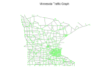
(a)

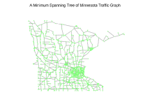
(b)

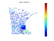
(c)

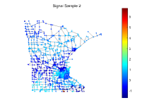
(d)

Figure 4: An illustration of Minnesota traffic graph, one of its minimum spanning tree and 2 signal samples from the family $\mathcal{F}$.

Signals from this family are generated by sampling $a_{i}$ from the Guassian distribution and following the evaluation as above (see Figure 4). We generate $50$ signals for training and $5$ signals for testing.

For the following tasks of non-linear approximation and denoising, we choose the following methods as baselines:

• Eigenvectors of unnormalized graph Laplacian $\bm{L}:=\bm{D}-\bm{W}$ (abbreviated as UL).

• Eigenvectors of normalized graph Laplacian $\tilde{\bm{L}}:=\bm{I}-\bm{D}^{-1/2}\bm{W}\bm{D}^{-1/2}$ (abbreviated as NL).

• GraphSS [13].

• GraphBior [5].

For GraphSS and GraphBior, we adopt the publicly released MATLAB code. In detail, we select “orth” filters and a 3-level decomposition of GraphSS, which results in an orthonormal basis. For GraphBior, we use the same configuration as in the file Biorth_filter bank_demo_2.m, which results in a biorthogonal basis.

The implementation of our method is written in Python. To construct a partition tree for Minnesota traffic graph, we adopt the Python package scikit-network and apply a step of post-processing to perform a series of clustering on graphs as described at the beginning of Section II-C. Eventually, we obtain a partition tree with $J=3$, in which each non-leaf node has no less than $15$ children, i.e. $|\mathcal{C}_{j,k}|\geq 15$. This allows choosing large enough $r_{j}$ for $\bm{A}^{[j,k]}$ and thus allows varying the dimension of $\mathbb{V}_{0}$. To obtain a $M$-dimensional $\mathbb{V}_{0}$, we set $r_{J-1}=M$ and the rest $r_{j}$ are set to $1$. As for solving the optimization problem in (24) and the modified version of the optimization problem in (25), we adopt the Python package pymanopt[49] and apply conjugate gradient method on Riemannian manifolds. The configuration is set to default and a summary of time consumed is presented in Table I. Figures of graphs are generated using GSPBOX [50].

TABLE I: Time consumed on solving Riemannian optimization problems.

Variant	Time (Unit: second)
$\mathsf{GIB}$-1$(1)$	1002.03
$\mathsf{GIB}$-1$(4)$	1001.59
$\mathsf{GIB}$-1$(8)$	1002.45
$\mathsf{GIB}$-1$(12)$	1002.44
$\mathsf{GIB}$-2$(1,20)$	1158.92
$\mathsf{GIB}$-2$(4,20)$	1147.13
$\mathsf{GIB}$-2$(1,50)$	1388.68
$\mathsf{GIB}$-2$(4,50)$	1350.72
$\mathsf{GIB}$-2$(1,100)$	1772.85
$\mathsf{GIB}$-2$(4,100)$	1629.42
$\mathsf{GIF}$-2$(1,20)$	1366.11
$\mathsf{GIF}$-2$(4,20)$	1307.43

V-B Non-linear Approximation

In this subsection, we choose only bases constructed from our method, e.g., $\mathsf{GIB}$-1$(4)$. To conduct non-linear approximation (NLA) on a signal $\bm{f}$ using top-$N$ coefficients of a dictionary $\mathcal{D}:=\{\bm{g}_{1},\bm{g}_{2},\dots,\bm{g}_{n}\}\subset\mathbb{R}^{n}$, we sort the coefficients $c_{i}:=\langle\bm{f},\bm{g}_{i}\rangle$ decreasingly according to $|c_{i}|$ and keep the top-$N$ coefficients. The remaining ones are set to $0$. Then a signal $\tilde{\bm{f}}$ is reconstructed according to these modified coefficients using the proper inverse operator. We report the relative error, i.e., $\|\bm{f}-\tilde{\bm{f}}\|/\|\bm{f}\|$.

V-B1 Comparison among Variants

Here, we compare the results among variants with different dimensions of $\mathbb{V}_{0}$. The NLA is performed on one of 5 test signals. As shown in Figure 5, when the dimension is $4$, the learned $\mathbb{V}_{0}$ best fit the family $\mathfrak{F}$ and produces the sparsest representation for the test signal, indicating a low-dimensional structure of $\mathfrak{F}$ with a dimension larger than 1. On the other hand, for the cases of dimensions 8 and 12, the results indicate a surplus in defining the size of $\mathbb{V}_{0}$, which distributes the energy of signal over an excessive set and thus results in a denser representation. In contrast, the one-dimension case generally has the densest representation since a one-dimensional $\mathbb{V}_{0}$ is insufficient in fitting the low-dimensional structure of $\mathfrak{F}$.

Figure 5: Relative Error of 4 variants.

Given the observation above, we further compare the two extreme cases, i.e. $\mathsf{GIB}$-1$(1)$ and $\mathsf{GIB}$-1$(4)$, for which optimize the filters $\bm{B}^{[j,k]}$ as well. The NLA is performed on the same test signal. As shown in Figure 6, optimizing $\bm{B}^{[j,k]}$ gives sparser representations. For $\mathsf{GIB}$-1$(4)$, the results of optimizing top-20, 50, and 100 subspaces are indistinguishable since the 4-dimensional $\mathbb{V}_{0}$ has conversed most of the energy and thus it requires only a small portion of subspaces to optimize.

On the contrary, for $\mathsf{GIB}$-1$(1)$, there is a great portion of energy distributed outside of the 1-dimensional $\mathbb{V}_{0}$. Thus, it requires more subspaces to optimize. Only when 100 subspaces are optimized, i.e., $\mathsf{GIB}$-2$(1,100)$, does the 1-dimensional case achieve a performance comparable with the 4-dimensional case, i.e., $\mathsf{GIB}$-2$(4,20)$.

In conclusion, selecting a proper order of generalized vanishing moments at the beginning provides more efficient and economic optimization in obtaining $\bm{B}^{[j,k]}$.

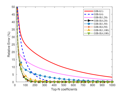
Figure 6: Relative Error of 8 variants.

V-B2 Comparison with Baselines

Based on the aforementioned results, we select $\mathsf{GIB}$-2$(1,20)$ and $\mathsf{GIB}$-2$(4,20)$ to compare with the baselines. We report the average relative error of the 5 test signals. As shown in Figure 7, $\mathsf{GIB}$-2$(4,20)$ evidently outperforms all other methods.

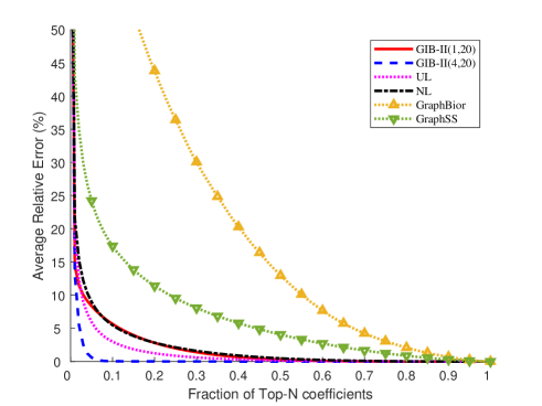
Figure 7: Average Relative Error of All Methods.

V-C Denoising

In this subsection, we include two more variants $\mathsf{GIF}$-2$(1,20)$ and $\mathsf{GIF}$-2$(4,20)$ to compare with the baselines.

For each test signal, we add Gaussian noise with $\sigma=1/16,1/8,1/4$ and $1/2$. Then, the coefficients are thresholded with a threshold value set as $3\sigma$. We report the signal-to-noise ratio (SNR). The results are shown in Table II.

Our method surpasses the baselines by a large margin. A sparser representation is better for denoising since more coefficients are dominated by noise, and thus thresholding such coefficients results in less loss of the origin signal. Moreover, we mention in the introduction that frames have the potential to perform better since the energy of noise is distributed over more atoms, resulting in smaller coefficients. With the current setting, as shown in the last column of Table II, this happens when the noise is large enough. In other cases, their performance is very close to the bases.

TABLE II: Average SNR. Best in bold. Unit: dB.

Method	$\sigma=1/16$	$\sigma=1/8$	$\sigma=1/4$	$\sigma=1/2$
UL	17.97	13.92	10.46	7.54
NL	16.51	12.29	9.2	6.54
GraphBior	9.59	6.06	2.76	0.88
GraphSS	8.92	6.18	3.73	1.76
$\mathsf{GIB}$-2$(1,20)$	17.32	12.37	9.49	7.58
$\mathsf{GIB}$-2$(4,20)$	25.31	20.15	14.67	9.62
$\mathsf{GIF}$-2$(1,20)$	16.6	12.16	9.6	7.91
$\mathsf{GIF}$-2$(4,20)$	25.24	20.03	14.67	10.32

VI Conclusion and Discussion

Our proposed method of constructing tight graph framelet systems is parameterized, general, and flexible in adjusting the space of scaling functions, resulting in locally supported framelets associated with fast forward and backward transforms and possessing generalized vanishing moments.

By learning the space $\mathbb{V}_{0}$ to capture the low-dimensional structure of a family of signals and learning the optimal bases/frames of the subspaces orthogonal to $\mathbb{V}_{0}$, our method can provide far more sparser representations compared with other non-data-adapted approaches. Such sparseness is reflected in the superior performance of non-linear approximation and denoising tasks.

The training time in solving the Riemannian optimization problems could be an issue. We would like to point out that some of the filters $\bm{A}^{[j,k]}$ can be predefined to reduce the number of parameters and, consequently, the training overhead. In this case, the system has a smaller representation capacity.

As for further applications, given a pre-trained system, the fast forward and backward transforms resemble the computation in general neural networks and can be combined with a properly defined neural network. Using its sparseness, a pre-trained system can serve as a regularizer in deep learning tasks. It can also applied in compressed sensing. These remain future directions to be explored.

Finally, our method can be applied to more general discrete and irregular data as long as a series of partitions is given. Thus, apart from graph data, it has the potential to be applied in more complicated settings.

References

• [1] D. I. Shuman, S. K. Narang, P. Frossard, A. Ortega, and P. Vandergheynst, “The emerging field of signal processing on graphs: Extending high-dimensional data analysis to networks and other irregular domains,” IEEE Signal Processing Magazine, vol. 30, no. 3, pp. 83–98, 2013.
• [2] A. Ortega, P. Frossard, J. Kovačević, J. M. Moura, and P. Vandergheynst, “Graph signal processing: Overview, challenges, and applications,” Proceedings of the IEEE, vol. 106, no. 5, pp. 808–828, 2018.
• [3] F. R. Chung, Spectral Graph Theory.   American Mathematical Soc., 1997, vol. 92.
• [4] S. K. Narang and A. Ortega, “Perfect reconstruction two-channel wavelet filter banks for graph structured data,” IEEE Transactions on Signal Processing, vol. 60, no. 6, pp. 2786–2799, 2012.
• [5] ——, “Compact support biorthogonal wavelet filterbanks for arbitrary undirected graphs,” IEEE Transactions on Signal Processing, vol. 61, no. 19, pp. 4673–4685, 2013.
• [6] A. Sakiyama and Y. Tanaka, “Oversampled graph laplacian matrix for graph filter banks,” IEEE Transactions on Signal Processing, vol. 62, no. 24, pp. 6425–6437, 2014.
• [7] H. Q. Nguyen and M. N. Do, “Downsampling of signals on graphs via maximum spanning trees,” IEEE Transactions on Signal Processing, vol. 63, no. 1, pp. 182–191, 2014.
• [8] X. Zheng, Y. Y. Tang, and J. Zhou, “A framework of adaptive multiscale wavelet decomposition for signals on undirected graphs,” IEEE Transactions on Signal Processing, vol. 67, no. 7, pp. 1696–1711, 2019.
• [9] J. You and L. Yang, “Perfect reconstruction two-channel filter banks on arbitrary graphs,” Applied and Computational Harmonic Analysis, vol. 65, pp. 296–321, 2023.
• [10] E. Pavez, B. Girault, A. Ortega, and P. A. Chou, “Two channel filter banks on arbitrary graphs with positive semi definite variation operators,” IEEE Transactions on Signal Processing, vol. 71, pp. 917–932, 2023.
• [11] S. Li, Y. Jin, and D. I. Shuman, “Scalable $m$-channel critically sampled filter banks for graph signals,” IEEE Transactions on Signal Processing, vol. 67, no. 15, pp. 3954–3969, 2019.
• [12] N. Tremblay and P. Borgnat, “Subgraph-based filterbanks for graph signals,” IEEE Transactions on Signal Processing, vol. 64, no. 15, pp. 3827–3840, 2016.
• [13] A. Sakiyama, K. Watanabe, Y. Tanaka, and A. Ortega, “Two-channel critically sampled graph filter banks with spectral domain sampling,” IEEE Transactions on Signal Processing, vol. 67, no. 6, pp. 1447–1460, 2019.
• [14] M. S. Kotzagiannidis and P. L. Dragotti, “Splines and wavelets on circulant graphs,” Applied and Computational Harmonic Analysis, vol. 47, no. 2, pp. 481–515, 2019.
• [15] A. Miraki and H. Saeedi-Sourck, “Spline graph filter bank with spectral sampling,” Circuits, Systems, and Signal Processing, vol. 40, no. 11, pp. 5744–5758, 2021.
• [16] ——, “A modified spline graph filter bank,” Circuits, Systems, and Signal Processing, vol. 40, pp. 2025–2035, 2021.
• [17] V. N. Ekambaram, G. C. Fanti, B. Ayazifar, and K. Ramchandran, “Spline-like wavelet filterbanks for multiresolution analysis of graph-structured data,” IEEE Transactions on Signal and Information Processing over Networks, vol. 1, no. 4, pp. 268–278, 2015.
• [18] J. You and L. Yang, “Spline-like wavelet filterbanks with perfect reconstruction on arbitrary graphs,” IEEE Transactions on Signal and Information Processing over Networks, 2023.
• [19] D. K. Hammond, P. Vandergheynst, and R. Gribonval, “Wavelets on graphs via spectral graph theory,” Applied and Computational Harmonic Analysis, vol. 30, no. 2, pp. 129–150, 2011.
• [20] B. Dong, “Sparse representation on graphs by tight wavelet frames and applications,” Applied and Computational Harmonic Analysis, vol. 42, no. 3, pp. 452–479, 2017.
• [21] H. Behjat, U. Richter, D. Van De Ville, and L. Sörnmo, “Signal-adapted tight frames on graphs,” IEEE Transactions on Signal Processing, vol. 64, no. 22, pp. 6017–6029, 2016.
• [22] N. Leonardi and D. Van De Ville, “Tight wavelet frames on multislice graphs,” IEEE Transactions on Signal Processing, vol. 61, no. 13, pp. 3357–3367, 2013.
• [23] D. B. Tay, Y. Tanaka, and A. Sakiyama, “Almost tight spectral graph wavelets with polynomial filters,” IEEE Journal of Selected Topics in Signal Processing, vol. 11, no. 6, pp. 812–824, 2017.
• [24] M. Crovella and E. Kolaczyk, “Graph wavelets for spatial traffic analysis,” in IEEE INFOCOM 2003. Twenty-second Annual Joint Conference of the IEEE Computer and Communications Societies (IEEE Cat. No. 03CH37428), vol. 3.   IEEE, 2003, pp. 1848–1857.
• [25] M. Gavish, B. Nadler, and R. R. Coifman, “Multiscale wavelets on trees, graphs and high dimensional data: Theory and applications to semi supervised learning,” in ICML, 2010.
• [26] C. K. Chui, F. Filbir, and H. N. Mhaskar, “Representation of functions on big data: graphs and trees,” Applied and Computational Harmonic Analysis, vol. 38, no. 3, pp. 489–509, 2015.
• [27] C. K. Chui, H. Mhaskar, and X. Zhuang, “Representation of functions on big data associated with directed graphs,” Applied and Computational Harmonic Analysis, vol. 44, no. 1, pp. 165–188, 2018.
• [28] J. Li, R. Zheng, H. Feng, M. Li, and X. Zhuang, “Permutation Equivariant Graph Framelets for Heterophilous Graph Learning,” arXiv e-prints, p. arXiv:2306.04265, Jun. 2023.
• [29] B. Han, “Framelets and wavelets,” Algorithms, Analysis, and Applications, Applied and Numerical Harmonic Analysis. Birkhäuser xxxiii Cham, 2017.
• [30] I. Daubechies, Ten Lectures on Wavelets.   SIAM, 1992.
• [31] S. Mallat, A Wavelet Tour of Signal Processing: The Sparse Way.   Academic Press, 2008.
• [32] E. J. Candès and D. L. Donoho, “New tight frames of curvelets and optimal representations of objects with piecewise $c^{2}$ singularities,” Communications on Pure and Applied Mathematics: A Journal Issued by the Courant Institute of Mathematical Sciences, vol. 57, no. 2, pp. 219–266, 2004.
• [33] G. Kutyniok and D. Labate, “Introduction to shearlets,” Shearlets: Multiscale Analysis for Multivariate Data, pp. 1–38, 2012.
• [34] B. Han and X. Zhuang, “Smooth affine shear tight frames with mra structure,” Applied and Computational Harmonic Analysis, vol. 39, no. 2, pp. 300–338, 2015.
• [35] B. Han, Z. Zhao, and X. Zhuang, “Directional tensor product complex tight framelets with low redundancy,” Applied and Computational Harmonic Analysis, vol. 41, no. 2, pp. 603–637, 2016.
• [36] X. Zhuang, “Digital affine shear transforms: fast realization and applications in image/video processing,” SIAM Journal on Imaging Sciences, vol. 9, no. 3, pp. 1437–1466, 2016.
• [37] Z. Che and X. Zhuang, “Digital affine shear filter banks with 2-layer structure and their applications in image processing,” IEEE Transactions on Image Processing, vol. 27, no. 8, pp. 3931–3941, 2018.
• [38] B. Han, T. Li, and X. Zhuang, “Directional compactly supported box spline tight framelets with simple geometric structure,” Applied Mathematics Letters, vol. 91, pp. 213–219, 2019.
• [39] B. Han, Q. Mo, Z. Zhao, and X. Zhuang, “Directional compactly supported tensor product complex tight framelets with applications to image denoising and inpainting,” SIAM Journal on Imaging Sciences, vol. 12, no. 4, pp. 1739–1771, 2019.
• [40] N. Sharon and Y. Shkolnisky, “A class of laplacian multiwavelets bases for high-dimensional data,” Applied and Computational Harmonic Analysis, vol. 38, no. 3, pp. 420–451, 2015.
• [41] J. Li, H. Feng, and X. Zhuang, “Convolutional neural networks for spherical signal processing via area-regular spherical haar tight framelets,” IEEE Transactions on Neural Networks and Learning Systems, 2022.
• [42] S. G. Mallat, “A theory for multiresolution signal decomposition: the wavelet representation,” IEEE Transactions on Pattern Analysis and Machine Intelligence, vol. 11, no. 7, pp. 674–693, 1989.
• [43] A. Ron and Z. Shen, “Affine systems in ${L_{2}(R^{d})}$: the analysis of the analysis operator,” Journal of Functional Analysis, vol. 148, no. 2, pp. 408–447, 1997.
• [44] X. Zheng, B. Zhou, Y. G. Wang, and X. Zhuang, “Decimated framelet system on graphs and fast g-framelet transforms,” The Journal of Machine Learning Research, vol. 23, no. 1, pp. 787–854, 2022.
• [45] P.-A. Absil, R. Mahony, and R. Sepulchre, Optimization Algorithms on Matrix Manifolds.   Princeton University Press, 2008.
• [46] Y. G. Wang and X. Zhuang, “Tight framelets and fast framelet filter bank transforms on manifolds,” Applied and Computational Harmonic Analysis, vol. 48, no. 1, pp. 64–95, 2020.
• [47] N. T. Trendafilov, “On the $l_{1}$ procrustes problem,” Future Generation Computer Systems, vol. 19, no. 7, pp. 1177–1186, 2003.
• [48] G. Freud, Orthogonal Polynomials.   Elsevier, 2014.
• [49] J. Townsend, N. Koep, and S. Weichwald, “Pymanopt: A python toolbox for optimization on manifolds using automatic differentiation,” Journal of Machine Learning Research, vol. 17, no. 137, pp. 1–5, 2016.
• [50] N. Perraudin, J. Paratte, D. Shuman, L. Martin, V. Kalofolias, P. Vandergheynst, and D. K. Hammond, “Gspbox: A toolbox for signal processing on graphs,” arXiv preprint arXiv:1408.5781, 2014.