Dynamic Frame Interpolation in Wavelet Domain
Abstract
Video frame interpolation is an important low-level vision task, which can increase frame rate for more fluent visual experience. Existing methods have achieved great success by employing advanced motion models and synthesis networks. However, the spatial redundancy when synthesizing the target frame has not been fully explored, that can result in lots of inefficient computation. On the other hand, the computation compression degree in frame interpolation is highly dependent on both texture distribution and scene motion, which demands to understand the spatial-temporal information of each input frame pair for a better compression degree selection. In this work, we propose a novel two-stage frame interpolation framework termed WaveletVFI to address above problems. It first estimates intermediate optical flow with a lightweight motion perception network, and then a wavelet synthesis network uses flow aligned context features to predict multi-scale wavelet coefficients with sparse convolution for efficient target frame reconstruction, where the sparse valid masks that control computation in each scale are determined by a crucial threshold ratio. Instead of setting a fixed value like previous methods, we find that embedding a classifier in the motion perception network to learn a dynamic threshold for each sample can achieve more computation reduction with almost no loss of accuracy. On the common high resolution and animation frame interpolation benchmarks, proposed WaveletVFI can reduce computation up to 40% while maintaining similar accuracy, making it perform more efficiently against other state-of-the-arts. Code is available at https://github.com/ltkong218/WaveletVFI.
Index Terms:
Video frame interpolation, wavelet transform, dynamic neural networks, adaptive inference, high efficiency.I Introduction
Video frame interpolation (VFI) is an important low-level computer vision task aiming to generate non-exist intermediate frames between actual successive inputs, which can largely increase the video temporal resolution. It plays an important role in broad application prospects, such as slow motion generation [1], video editing [2], animation production [3] and frame rate up-conversion [4, 5].
The successful flow-based frame interpolation algorithms [6, 1, 7, 8] can mostly be abstracted as two-stage encoder-decoder architectures, that first model optical flow between target frame and input frames, and then generate the target frame by a synthesis network. To improve the first stage, current state-of-the-arts try to adopt higher order motion model [9, 10, 11], additional refinement unit [9, 12] or directly estimate intermediate flow by a learnable network [13, 14, 15]. As for the second stage, more powerful synthesis networks are employed to improve the frame generation ability [6, 8, 16, 17]. Although significant progresses have been made by above flow-based approaches, their static deep architectures can lead to large computation redundancy on the typical piecewise flat regions in high resolution and animation videos, restricting their application scenarios to a great extent.

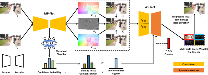
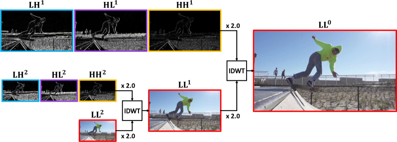
In this paper, inspired by the sparse representation in wavelet decomposition, we propose a novel two-stage flow-based frame interpolation algorithm called WaveletVFI for higher computation efficiency. Different from previous methods that directly synthesize the target frame in RGB color space [7, 8, 17, 12], we employ discrete wavelet transform (DWT) to decompose the target frame into multi-scale frequency domain and propose a wavelet synthesis network (WS-Net) to predict the decomposed wavelet coefficients which are inherently sparse in high resolution or cartoon images. For wavelet coefficients, the low-frequency component represents the overall scene structure and the sparse high-frequency component describes some edge information. During the progressive inverse discrete wavelet transform (IDWT) based image reconstruction procedure, only the sparse high-frequency components need to be estimated in this scale. Therefore, as shown in Fig. 1, we can employ efficient sparse convolution decoder in WS-Net to predict multi-scale high-frequency wavelet coefficients only in certain areas, while still enabling high-quality intermediate frame synthesizing.
In order to build the valid spatial mask for sparse convolution, a threshold ratio has to be determined, like the quantization step in image compression [18, 19]. Admittedly, the threshold hyper-parameter is an important factor that affects the computation cost and the VFI accuracy. As depicted in Fig. 1, for the same WS-Net, a lower threshold ratio will keep more high-frequency coefficients to be estimated, resulting in larger computation and usually higher accuracy. In contrast, more high-frequency coefficients are ignored and set to zero, often yielding lower performance while the required computation are also smaller. Thus, how to set a reasonable threshold is worth studying, that has been widely discussed in traditional image compression and denoising tasks [20, 21]. However, in VFI task, the scene content to be generated comes from dynamic inputs, making the compression threshold for synthesizing the intermediate frame highly dependent on both texture distribution and motion situation of each input frame pair, which are difficult to be modeled explicitly. For example, given input frames with clear texture and from certain inter-frame motion, more high-frequency coefficients should be kept for better accuracy. On the other hand, when feeding input frames with blurry texture or from uncertain motion, more high-frequency coefficients can be ignored to save computation but without perceptible accuracy loss.
To deal with this problem, we propose a novel dynamic threshold ratio selection approach which can adjust the computation cost compression degree of each input sample adaptively for more efficient inference. Specifically, we introduce a threshold classifier which is embedded in the bottom part of the first stage motion perception network (MP-Net) and can learn the spatial-temporal information existed in input frames. In practice, we set several different threshold ratios as candidates and use output probability distribution over candidates of the threshold classifier as selection guidance. The MP-Net together with the threshold classifier are carefully designed with lightweight model size and computation complexity, and are jointly optimized with WS-Net for VFI task in an end-to-end manner. By exploiting the proposed dynamic compression threshold selection approach, we can better excavate computation redundancy when synthesizing the compressible target frame.
In summary, to our best knowledge, we are the first to explore the spatial redundancy problem in frame interpolation, and further build a deep VFI architecture in wavelet domain for efficient inference. Moreover, we propose a novel dynamic threshold selection mechanism to better allocate computation for each input sample. Experiments on the traditional Vimeo90K [13], the animation ATD12K [3] and the high resolution Xiph-2K [22] and Xiph-4K [22] frame interpolation benchmarks demonstrate the effectiveness of proposed approaches, which can adaptively reduce the overall resource consumption while maintaining advanced VFI accuracy.
II Related Work
II-A Video Frame Interpolation
Research in deep learning based frame interpolation can be roughly categorized into flow-based and kernel-based approaches. Kernel-based methods adopt adaptive convolution [23], where they unify motion estimation and frame generation into a single convolution step with spatial varying convolution kernels. Following works mainly enhance the freedom of convolution operation [24, 25, 26], combining optical flow offsets for better spatial alignment [27], or introducing channel attention mechanism [28]. Kernel-based approaches can naturally generate complex contextual details, however, their prediction tend to be blurry when scene motion is large.
Recent state-of-the-arts mostly adopt flow-based methods [1, 7, 9, 8, 3, 17, 12, 29, 30, 31], since optical flow can provide an explicit correspondence for frame registration, especially in large motion scenes. Due to there is an independent motion modeling step in flow-based approaches, they usually contain a second target frame synthesizing stage. Existing improvement for the first stage try to adopt more advanced motion model [9, 10, 11, 30], additional refinement unit [9, 12] or directly estimate intermediate flow by an encoder-decoder network [13, 14, 15]. As for the second stage, more powerful synthesis networks are employed to improve the frame generation ability [6, 8, 16, 17].
In order to achieve more efficiency, CDFI [32] first leverages model pruning through sparsity-inducing optimization, and then add additional synthesis module to improve previous compressed network, which significantly reduces model size against the baseline AdaCoF [25]. However, their complex architecture leads to large time delay and the results are inferior to current SOTA methods. Like our approach, CAIN-SD [33] also adopts a motion-aware dynamic architecture for efficiency, where they dynamically adjust the network depth and input resolution for each input image patch. However, their stitched target frame contains artifacts at patch edges, and their base model CAIN [28] can not deal with large motion as well as flow-based VFI methods. Recently, IFRNet [29] achieves state-of-the-art speed accuracy trade-off by jointly refining intermediate optical flow together with a powerful intermediate feature within a single encoder-decoder architecture. However, the fully convolutional structure treats each pixel for synthesizing equally, that can result in large computation redundancy when generating lots of smooth regions.
II-B Wavelets in Computer Vision
Wavelet decomposition and reconstruction is widely used in signal processing, image processing and computer vision. The discrete wavelet transform (DWT) can make the signal energy distribution more concentrated on principle frequency components and hence compress redundant information. The JPEG2000 [34, 35] standard employs DWT algorithm in the image compression stage, and a truncated threshold plays a key role for quantization [20, 21]. The frequency filtering characteristic of wavelet transform is also applied on traditional image denoising task [36, 21].
Recently, wavelet transform has been combined with diverse deep learning based computer vision tasks. WDNet [37] proposes to remove image moiré artifacts in the wavelet domain, which is difficult to distinguish from true texture in the RGB color space. Some super-resolution methods [38, 39, 40] learn to estimate multiple high-frequency wavelet coefficients from a low-resolution input image to generate high-resolution image by inverse discrete wavelet transform (IDWT). WaveletStereo [41] learns stereo matching by predicting the wavelet coefficients of the disparity, that can better deal with global context with textureless surfaces. Closer to our work, WaveletMonodepth [42] predicts multi-scale sparse wavelet coefficients for efficient monocular depth estimation. However, their compression threshold value can not dynamically adjust on every sample for better accuracy efficiency trade-off. Moreover, the threshold selection in dynamic VFI task is more complex than the static monocular depth task, since motion uncertainty will influence the compression characteristic curve. To our best knowledge, we are the first to apply wavelet transform to frame interpolation, and further in a dynamic manner.
II-C Dynamic Neural Networks
Dynamic neural networks, as opposed to traditional static models, can adapt their structures or parameters according to the input during inference, and therefore enjoy favorable properties that are absent in static ones. One of the most notable advantages of dynamic models is that they are able to allocate computations on demand in test time. Common practices mostly include dynamic depth, dynamic width and spatial-wise dynamic networks. The dynamic depth approaches contain two major types of early exiting [45, 46] and layer skipping [47, 48]. The dynamic width networks usually skip neurons in fully-connected (FC) layers [49, 50] or skip channels in convolutional neural networks (CNNs) [51, 52]. The spatial-wise dynamic networks often leverage dynamic sparse convolution to reduce the unnecessary computation on less informative locations, where our WaveletVFI falls into this category. To determine the spatial location for sparse convolution, diverse sampling strategies are invented. A typical approach is to use an extra network branch to generate a spatial valid mask where many methods [53, 54, 55] belong to this paradigm. Another kind algorithms make use of the sparse characteristics of the input [56]. Different from these methods, our approach leverages the intrinsic sparsity of wavelet representation and explore the optimal sparsity degree by learning from the spatial-temporal motion information in an end-to-end manner, that is especially suitable for frame interpolation task.
III Method
In this section, we first introduce the overall framework of the proposed method. Then, we describe the bidirectional intermediate flow estimation and dynamic compression threshold selection approach in motion perception network. Further, complementary context encoder, sparse convolution decoder and progressive IDWT based target frame reconstruction algorithm in wavelet synthesis network are demonstrated. Finally, we present the optimization procedure and loss functions.
III-A Framework Overview
Inspired by the sparse representation characteristic of wavelet decomposition and threshold selection methods on image compression [34, 20, 21], we propose an instance-aware dynamic compression threshold selection approach in wavelet domain for efficient video frame interpolation. As shown in Fig. 2, our proposed method follows the successful two-stage flow-based VFI pipeline. In the first stage, the MP-Net jointly estimates bidirectional intermediate flow and an occlusion fusion mask from coarse to fine. Then, the intermediate flow, occlusion mask, input images and merged intermediate frame are fed into the encoder part of WS-Net in the second stage. Meanwhile, the threshold classifier in MP-Net learns the spatial-temporal input information and provides candidates probability for compression threshold selection, which controls the computation cost and synthesis accuracy of the sparse convolution decoder part of WS-Net. In training, candidates probability is applied with Gumbel softmax trick [43, 44] for gradient back propagation, while in inference, only threshold ratio with maximum probability is selected for synthesizing.
III-B Motion Perception Network
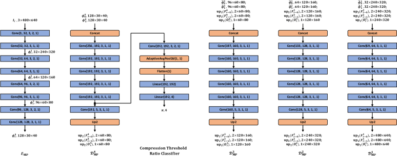
III-B1 Joint Intermediate Flow and Occlusion Estimation
The MP-Net takes two input frames and jointly estimates bidirectional intermediate optical flow with occlusion fusion mask in a coarse-to-fine manner. Specifically, the pyramid encoder of MP-Net extracts 4 levels of pyramid features, i.e., and from and respectively, where the spatial resolution of level is of level . The bottom level decoder directly takes the concatenation of as input, and estimates a coarse intermediate flow and fusion mask . Following the success of pyramid methods [57, 58, 59] in large displacement optical flow estimation, we adopt the 2 upsampled intermediate flow to backward warp pyramid features and obtained the warped features respectively. Then, the concatenated features of and are fed to decoder for estimating finer intermediate flow and occlusion mask . This procedure is performed recursively until reaching the original input resolution and yielding . In experiments, we find that integrate occlusion mask with intermediate flow for joint refinement can provide more useful information for the following synthesis network with negligible additional cost. Concretely, we can build a merged intermediate frame to better guide the following WS-Net by
| (1) | ||||
| (2) |
where means backward warping, stands for element-wise multiplication, and is element-wise subtraction. Fig. 3 shows structure details of the motion perception network .
III-B2 Compression Threshold Classifier
The role of our proposed compression threshold ratio classifier, abbreviated as threshold classifier, is to decide the threshold ratio hyper-parameter for the following WS-Net, which controls the trade-off between computation complexity and target frame synthesis accuracy. However, different from the image compression [35, 20] and monocular depth estimation [42] tasks in wavelet domain, where the compression threshold is mainly affected by static scene content, in frame interpolation, the compression degree of target frame is influenced by both scene structure and motion situation, which are more complex to model. For example, target frames synthesized from input samples with blur, exposure and other noisy texture in the challenging motion scenes usually contain more unreliable high-frequency texture, which are more compressible and can even achieve better results by the denoising characteristics of wavelet transform [60, 21]. On the other hand, target frame with rich texture and from certain motion should keep more high-frequency wavelet coefficients for better quantitative and qualitative results. To deal with above intractable problem, we introduce the threshold classifier in MP-Net to find an appropriate instance-aware threshold ratio by inferring a probability distribution over candidate threshold ratios. In practice, as shown in Fig. 3, the threshold classifier is a lightweight network with one convolution and two fully-connected layers separated by Leaky ReLU activation, that is embedded to the second last convolution layer of decoder in MP-Net. Taking threshold ratios of as candidates, the threshold classifier predicts a categorical distribution over them. Since there exists an non-differentiable problem in the process from the soft probability outputs to the hard one-hot selection , we leverage the Gumbel softmax trick [43, 44] to make the discrete decision differentiable during the gradient back propagation, which means the discrete candidate threshold selections can be drawn by using
| (3) |
where is an i.i.d Gumbel noise sample, which will not influence the highest entry of the original categorical probability distribution. During training, the derivative of above one-hot operation can be approximated by Gumbel softmax function that is both continuous and differentiable
| (4) |
where is a temperature parameter. When , samples from Gumbel softmax distribution become uniform. In contrast, when , samples from Gumbel softmax distribution become one-hot. In our experiments, we start at a high temperature of and anneal it to finally.
III-C Wavelet Synthesis Network
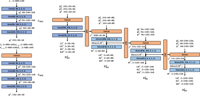
III-C1 Complementary Context Encoder
Like MP-Net, the WS-Net is also a U-shape encoder-decoder network, however, it has more feature channels but with less cascaded convolutions in each scale. The reason is that flow warped context features have almost been aligned to the target position, while more feature channels are needed for encoding diverse image texture. Different from previous methods [6, 8, 15] that adopt only a single encoder, we employ two different encoders to extract complementary context features. Specifically, extracts 4 levels of pyramid features of and from and separately. Then, they are warped by progressively down sampled intermediate flow fields to obtain target frame aligned context features of respectively. On the other hand, takes concatenation of and as input, and also extracts 4 levels of pyramid features of , that contain additional scene motion and occlusion information. Finally, we take the concatenated features of and as the complementary context feature in each level . Details of are depicted in Fig. 4.
III-C2 Haar Wavelet Transform
Before introducing sparse convolution decoder, we first explain the Haar wavelets used in our WaveletVFI, which has the simplest basis functions in discrete wavelet transform (DWT). Haar wavelet transform has four kernels, i.e., , where the low () and high () pass filters are
| (5) |
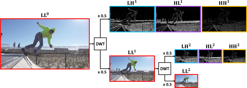
DWT with Haar wavelets can decompose a 2D image into four coefficient maps, including a low-frequency component and three high-frequency components at half the resolution of input image, where captures smooth texture while extract vertical, horizontal and diagonal ‘jump’ information. Since DWT is an invertible operation, we can adopt its inverse, i.e. IDWT, to convert four coefficient maps back to the 2D image at double the resolution of coefficient maps. To extract multi-scale and multi-frequency wavelet representation from ground truth intermediate frame , we can apply DWT operation recursively on the low-frequency coefficient map , starting from the input image , as shown in Fig. 5. Correspondingly, to reconstruct the predicted target frame , decoders in WS-Net , except the bottom one , only need to estimate three high-frequency wavelet coefficients in this scale, and apply IDWT operation on them recursively until reaching the original input resolution, that is shown in Fig. 6. Formally, these two mutually inverse transforms can be written as
| (6) | |||
| (7) |
where superscript denotes the current pyramid level, means the ground truth wavelet coefficients, and equals to ground truth frame and predicted target frame respectively.
III-C3 Sparse Convolution Decoder
For the piecewise flat regions in high resolution and cartoon images, most of their high-frequency wavelet coefficients have small values that are close to zero, while only some noticeable values are around image edges. Therefore, for full-resolution target frame reconstruction, only certain pixel locations need to estimate non-zero wavelet coefficients at each scale. Denoting these certain locations as sparse valid mask in level , where means valid, we can exploit sparse convolution to build decoder for efficient calculation as
| (8) |
where stands for the concatenated encoding and decoding pyramid features in level of the U-shape WS-Net. denotes the sparse valid mask of the last sparse convolution in decoder . To get meaningful value during sparse inference, we use the 33 morphological dilate operation to obtain the sparse valid mask of the first sparse convolution in each decoder . Given predicted multi-scale sparse wavelet coefficients, we can get the predicted intermediate frame , i.e., by exploiting inverse discrete wavelet transform (IDWT) progressively. It is worth noting that elements in the initial valid mask are all set to , and predicts an additional low-frequency coefficient .
III-C4 Sparse Valid Mask Calculation
Finally, we demonstrate how to calculate sparse valid mask in level , where the compression threshold ratio plays a key role as previously discussed. Inspired by the spatial correlation of different wavelet coefficient maps among multiple scales, which is first raised in the zerotree wavelets encoding algorithm [61], we assume that can be determined with high-frequency coefficient maps estimated at the previous scale by
| (9) |
Since the target frame is a 3-channel RGB image, we first calculate valid mask for each color channel, then we take the union set of as the final . As shown in Eq. 9, a larger will make more sparse, which usually leads to less computation and lower synthesis accuracy.
In summary, the target frame synthesis procedure in proposed WS-Net involves sparse valid mask calculation, sparse convolution inference and progressive IDWT based image reconstruction, we arrange these approaches into an algorithm for clarity which is presented in Algorithm 1.
III-D Optimization
III-D1 Differentiable Forward Propagation
Based on above analysis, the forward propagation stage of WaveletVFI can be summarized as following steps: 1) Given two input frames , predicts and a discrete candidate threshold selection by Gumbel softmax trick in Eq. 4. 2) Given and a specific candidate selection , estimates the multi-scale wavelet coefficients set , which is abbreviated as . 3) Denoting above progressive IDWT based target frame reconstruction algorithm as , the predicted intermediate frame based on the -th candidate selection can be obtained by . 4) Given the predicted candidate selection , we can get the final predicted target frame and multi-scale wavelet coefficients set by summing up with as follows
| (10) | ||||
| (11) |


III-D2 Loss Functions
For generating the target frame, we employ the same image reconstruction loss as IFRNet [29] between the prediction and ground truth , which is the sum of two terms as
| (12) |
where with is the robust Charbonnier loss [63]. is the census loss, which calculates soft Hamming distance between census-transformed image patches [64, 65]. Moreover, we adopt a new frequency domain reconstruction loss for better structure awareness as
| (13) |
where and are corresponding wavelet coefficient maps from the prediction set and the ground truth set , respectively. Finally, in order to reduce computation budget and balance different compression threshold ratio selection, we propose a computation cost regularization term as
| (14) |
where is the FLOPs counter, and represent the height and width of original input resolution. Our final objective function combines above three components with weighting parameters of and , where controls the trade-off between accuracy and efficiency, that is formulated as
| (15) |
IV Experiments
In this section, we first introduce the datasets used for training and test, and implementation details about the learning strategy. Then, we compare the proposed framework with recent state-of-the-art VFI methods on the commonly used low resolution, high resolution and animation frame interpolation benchmarks quantitatively and qualitatively. Finally, we carry out ablation study for analysis, and do more discussion.
IV-A Datasets
In this work, we supervise the proposed WaveletVFI on the training split of Vimeo90K [13], and test it on multiple datasets summarized as follows: 1) Vimeo90K [13] is a widely-used dataset for video processing tasks. There are 3,782 triplets with 448 256 resolution in the test set. 2) ATD12K [3] is an animation frame interpolation benchmark, where there are 2,000 triplets from diverse cartoon scenarios in test datasets. Note that we adopt the 960 540 resolution part to cover diverse video resolutions for more sufficient evaluation, which is different from the 1080p test part reported in the original paper. 3) Xiph [22] contains 30 raw video sequences that is originally used for testing video codecs. For frame interpolation, we follow the data processing operations in SoftSplat [8] to generate Xiph-2K test set by down sampling 4K videos and generate Xiph-4K test set by center cropping 2K patches. There are 392 frame triplets of resolution 2048 1080 in both Xiph-2K and Xiph-4K benchmarks.
the best result is boldfaced, and the second best is underlined.
| Method | Params | Vimeo90K | ATD12K | Xiph-2K | Xiph-4K | ||||||||
|---|---|---|---|---|---|---|---|---|---|---|---|---|---|
| (M) | TFLOPs | PSNR | SSIM | TFLOPs | PSNR | SSIM | TFLOPs | PSNR | SSIM | TFLOPs | PSNR | SSIM | |
| SepConv [24] | 21.7 | 0.108 | 33.79 | 0.970 | 0.487 | 27.40 | 0.950 | 2.078 | 34.77 | 0.929 | 2.078 | 32.06 | 0.880 |
| DAIN [7] | 24.0 | 0.686 | 34.71 | 0.976 | 3.099 | 27.38 | 0.955 | 13.22 | 35.97 | 0.940 | 13.22 | 33.51 | 0.898 |
| CAIN [28] | 42.8 | 0.162 | 34.65 | 0.973 | 0.734 | 25.28 | 0.952 | 3.133 | 35.21 | 0.937 | 3.133 | 32.56 | 0.901 |
| AdaCoF+ [25] | 22.9 | 0.282 | 34.56 | 0.959 | 1.273 | 27.39 | 0.937 | 5.433 | 35.09 | 0.931 | 5.433 | 32.19 | 0.882 |
| SoftSplat [8] | 12.2 | 0.112 | 36.10 | 0.970 | 0.506 | 28.22 | 0.957 | 2.160 | 36.62 | 0.944 | 2.160 | 33.60 | 0.901 |
| BMBC [16] | 11.0 | 0.311 | 35.06 | 0.964 | 1.405 | 27.68 | 0.945 | 5.994 | 32.82 | 0.928 | 5.994 | 31.19 | 0.880 |
| CDFI [32] | 5.0 | 0.102 | 35.17 | 0.964 | 0.463 | 28.15 | 0.950 | 1.977 | 35.50 | 0.960 | 1.977 | 32.50 | 0.932 |
| ABME [17] | 18.1 | 0.161 | 36.18 | 0.981 | 0.728 | 28.71 | 0.959 | 3.108 | 35.18 | 0.964 | 3.108 | 32.36 | 0.940 |
| CAIN-SD [33] | 42 | - | - | - | - | - | - | 1.598 | 34.68 | 0.924 | 1.983 | 32.92 | 0.893 |
| IFRNet-L [29] | 19.7 | 0.098 | 36.20 | 0.981 | 0.444 | 28.78 | 0.956 | 1.896 | 36.63 | 0.966 | 1.896 | 33.58 | 0.944 |
| WaveletVFI (Ours) | 19.4 | 0.081 | 35.58 | 0.978 | 0.274 | 28.79 | 0.956 | 1.480 | 36.32 | 0.965 | 1.428 | 33.61 | 0.945 |
GPU under PyTorch implementation.
| Method | DAIN | CAIN | AdaCoF+ | SoftSplat |
| Time (s) | 2.39 | 0.17 | 0.32 | 0.41 |
| Memory (GB) | 15.9 | 4.7 | 12.1 | 8.8 |
| Method | BMBC | CDFI | ABME | WaveletVFI |
| Time (s) | 9.10 | 0.92 | 1.63 | 0.19 |
| Memory (GB) | 27.2 | 27.9 | 17.2 | 7.0 |
IV-B Implementation Details
We implement the proposed WaveletVFI in PyTorch and adopt a two step learning schedule to train our algorithm on Vimeo90K training set from scratch. First, we train the and but without the threshold classifier for 300 epochs as initialization, where the compression threshold ratio is set to 0, weighting parameters and in Eq. 15 are set to 0.01 and 0 respectively. Then, we load the pre-trained parameters in step 1 and fine-tune the whole WaveletVFI framework with proposed dynamic threshold ratio selection approach for another 100 epochs to learn instance-aware threshold ratio selection, that considers the trade-off between accuracy and efficiency. In this stage, we set and to be 0.01 and 1 separately. All parameters that need to update are optimized by AdamW [66] algorithm, and the model is trained with total batch size 24 on four NVIDIA Tesla V100 GPUs. In both steps, the learning rate is initially set to , and gradually decays to following a cosine attenuation schedule. During training, we augment the triplet samples by random horizontal and vertical flipping, rotating, reversing sequence order and random cropping patches with size 256 256. Following the common practice of , all compared approaches only interpolate one middle frame in the experiments.
IV-C Comparison with the State-of-the-Arts
We compare proposed WaveletVFI with state-of-the-art VFI methods, including kernel-based SepConv [24], CAIN [28], AdaCoF [25], CDFI [32] and CAIN-SD [33], flow-based DAIN [7], SoftSplat [8], BMBC [16], ABME [17] and IFRNet [29]. Common metrics, such as Peak Signal-to-Noise Ratio (PSNR) and Structural Similarity (SSIM) [67] are adopted for quantitative evaluation. For the computation complexity, we calculate the number of floating-point operations (FLOPs) and average per sample FLOPs over specific dataset.
IV-C1 Quantitative Comparison
As shown in Table I, proposed approach always requires the smallest FLOPs than others, while achieving better or comparable accuracy. On the ATD12K [3] 540p animation benchmark, our method takes only 59% computation cost of the efficient CDFI [32], while obtaining 0.64 dB performance improvement. The method IFRNet [29] and ABME [17] also achieve similar accuracy as ours, however, proposed WaveletVFI only uses 62% or 38% multiply-add operations respectively with comparable model size. As for the high resolution Xiph [22] datasets, our approach performs best in both PSNR and SSIM on the more challenging Xiph-4K benchmark, while only falls behind IFRNet [29] and SoftSplat [8] on the Xiph-2K test set. Similar as ours, SoftSplat is also a two-stage flow-based frame interpolation method. However, thanks to the efficiency of proposed dynamic compression threshold selection approach in wavelet domain, we can achieve better or on par accuracy than SoftSplat, while requiring only 67% computation on the high resolution Xiph benchmarks. Compared with CAIN-SD [33], that is also a dynamic VFI method for reducing computation complexity, we achieve smaller FLOPs while obtaining significant accuracy gain, i.e., 1.64 dB better on Xiph-2K and 0.69 dB better on Xiph-4K. In regard to real deployment, as shown in Table II, we test inference time and peak GPU memory usage of several well-behaved VFI methods on one Tesla V100 GPU under PyTorch on Xiph-4K. It can be seen that proposed approach only falls behind CAIN [28] but outperforms others. Note that our sparse convolution is simulated by traditional convolution multiplied with sparse mask which supports end-to-end optimization in training. During inference, we follow the approach in WaveletMonodepth [42], and can replace it by more efficient operations.
In summary, considering 8 accuracy metrics, including PSNR and SSIM on Vimeo90K, ATD12K, Xiph-2K and Xiph-4K datasets, our approach ranks 1st 3 times, 2nd 1 times, and 3rd 3 times. Moreover, we always consume the least amount of computation. Above quantitative results have demonstrated the good comprehensive performance of our approaches.


| ID | Vimeo90K | |||||
|---|---|---|---|---|---|---|
| PSNR | SSIM | |||||
| E1 | ✓ | ✗ | ✗ | ✓ | 34.58 | 0.965 |
| E2 | ✗ | ✓ | ✗ | ✓ | 35.33 | 0.972 |
| E3 | ✓ | ✓ | ✗ | ✓ | 35.56 | 0.976 |
| E4 | ✓ | ✓ | ✓ | ✓ | 35.60 | 0.979 |
| E5 | ✓ | ✓ | ✗ | ✗ | 35.56 | 0.974 |
IV-C2 Qualitative Comparison
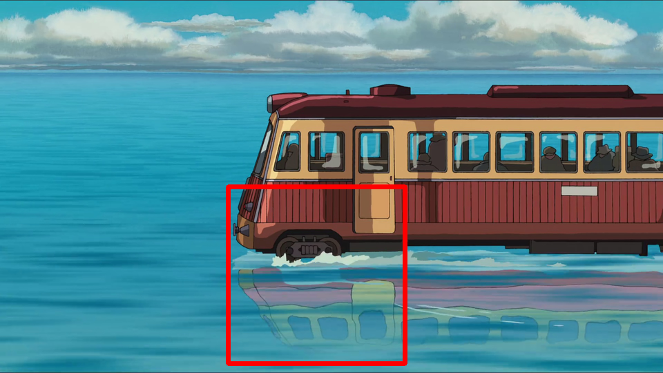
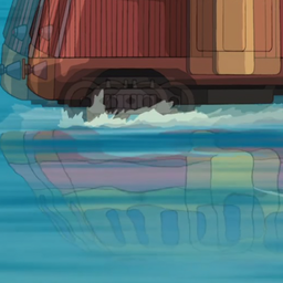
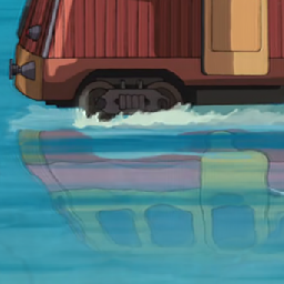
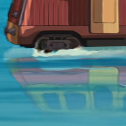
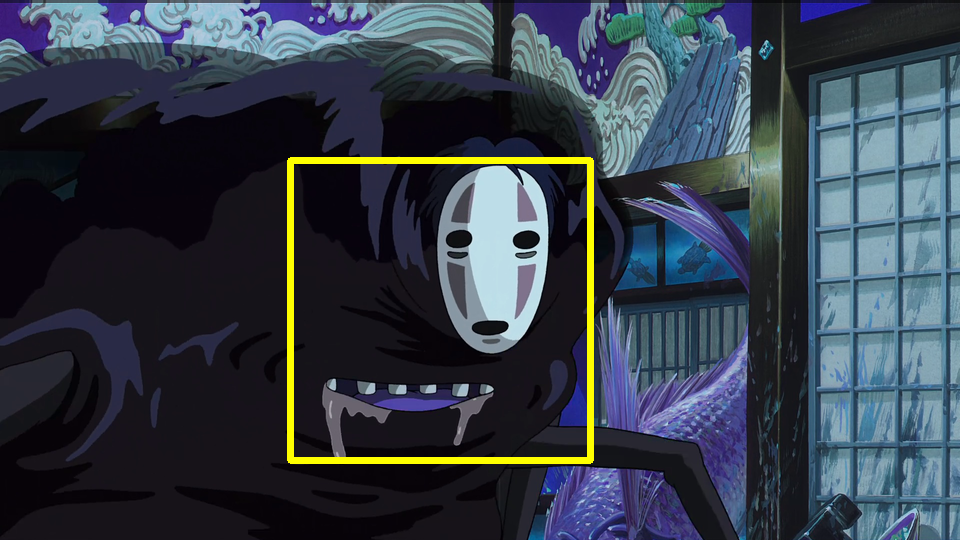
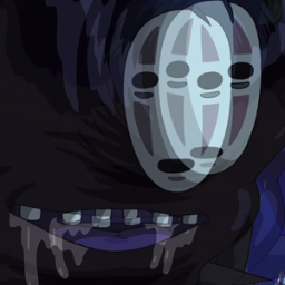
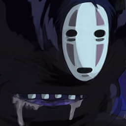
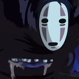
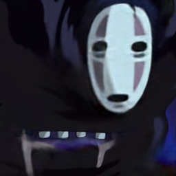
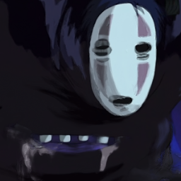
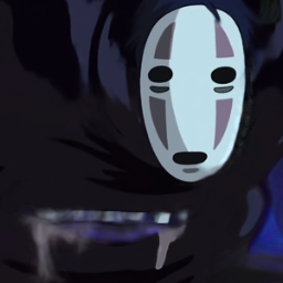
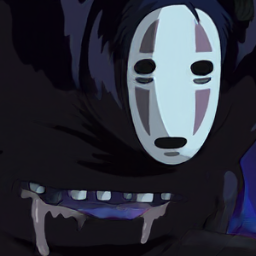
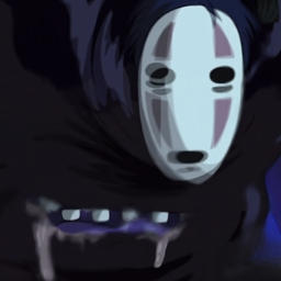
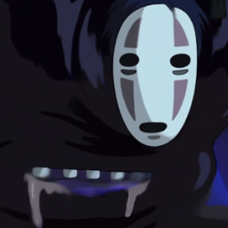
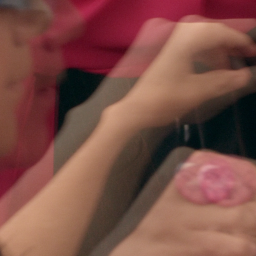
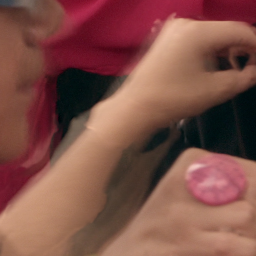
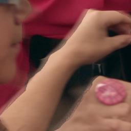
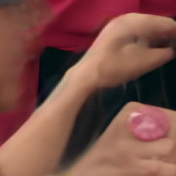
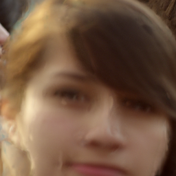
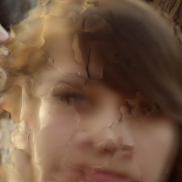
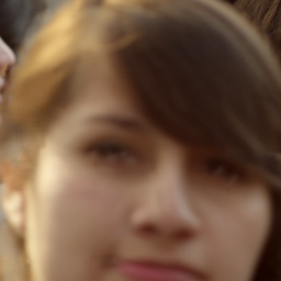
To visually compare with other SOTA methods, we show two examples from ATD12K and Xiph-4K in Fig. 7 and Fig. 8, respectively. The first example in Fig. 7 depicts a bus driving on the water, where proposed approach can synthesize the reflection of this cartoon bus realistically, while predictions from other methods behave blurry and twisty. The second example in Fig. 7 shows the character of No-Face in Spirited Away, where our method can generate clearer white face and more reasonable teeth. In Fig. 8, the first example shows a fast moving man waving his arm, which is a challenging case in Xiph-4K. It is obvious that proposed WaveletVFI can generate sharp motion boundary, while results of other methods contain ghosting artifacts. As for the second example in Fig. 8, interpolated frame of our approach looks more faithful and distinct.
IV-D Ablation Study
In this part, we analyze proposed contributions in network structure, loss function and hyper-parameters to explore the diverse characteristics of frame interpolation in wavelet domain and verify the effectiveness of proposed approaches.
IV-D1 Complementary Encoder, Frequency Loss and Wavelet Domain Interpolation
As shown in Table III, we carry out ablation to verify the effectiveness of complementary context encoders , frequency reconstruction loss and wavelet domain frame interpolation . We selectively remove or and enlarge feature channels of the remaining context encoder to be the same as original one for fair comparison. As listed in the first three rows of Table III, behaves more important than . It is because that jointly models scene texture, motion and occlusion, while is more focused on original contextual details. The combination of and achieves best results, demonstrating they are mutually benefit. Moreover, as listed of E4 in Table III, we can obtain better performance than E3 by introducing an additional frequency reconstruction loss . In this setting, improvement of SSIM is more obvious, verifying can help generate better scene structure. The last experiment E5 uses the same synthesis network structure but directly predicts target frame in color space. It concludes that frame interpolation in wavelet domain behaves a little better than in color space, verifying the rationality of progressive IDWT based target frame reconstruction for VFI.
| Dynamic | Vimeo90K | ATD12K | Xiph-2K | Xiph-4K | |||||||||
|---|---|---|---|---|---|---|---|---|---|---|---|---|---|
| TFLOPs | PSNR | SSIM | TFLOPs | PSNR | SSIM | TFLOPs | PSNR | SSIM | TFLOPs | PSNR | SSIM | ||
| ✗ | 0.0000 | 0.090 | 35.71 | 0.9791 | 0.409 | 28.83 | 0.9566 | 1.746 | 36.40 | 0.9664 | 1.746 | 33.62 | 0.9453 |
| ✗ | 0.0025 | 0.087 | 35.70 | 0.9789 | 0.346 | 28.83 | 0.9565 | 1.660 | 36.39 | 0.9662 | 1.666 | 33.61 | 0.9452 |
| ✗ | 0.0050 | 0.084 | 35.63 | 0.9780 | 0.314 | 28.82 | 0.9563 | 1.569 | 36.32 | 0.9646 | 1.558 | 33.58 | 0.9449 |
| ✗ | 0.0075 | 0.081 | 35.49 | 0.9762 | 0.289 | 28.80 | 0.9558 | 1.491 | 36.16 | 0.9620 | 1.465 | 33.51 | 0.9441 |
| ✗ | 0.0100 | 0.079 | 35.30 | 0.9738 | 0.270 | 28.78 | 0.9552 | 1.420 | 35.94 | 0.9587 | 1.385 | 33.43 | 0.9428 |
| ✗ | 0.0125 | 0.077 | 35.05 | 0.9709 | 0.256 | 28.76 | 0.9546 | 1.356 | 35.68 | 0.9557 | 1.316 | 33.32 | 0.9413 |
| ✗ | 0.0150 | 0.075 | 34.76 | 0.9675 | 0.245 | 28.73 | 0.9538 | 1.301 | 35.38 | 0.9528 | 1.256 | 33.19 | 0.9396 |
| Dataset | Vimeo90K | ATD12K | Xiph-2K | Xiph-4K |
|---|---|---|---|---|
| Mean Value | 6.06 | 19.4 | 10.9 | 25.3 |
| Standard Deviation | 6.12 | 32.3 | 12.5 | 33.3 |
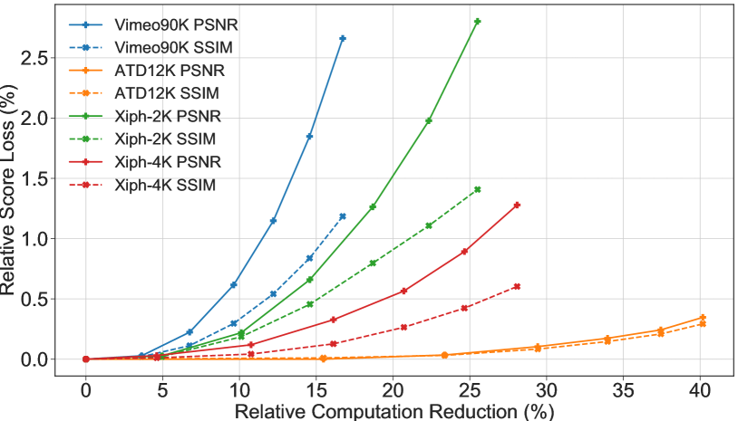
IV-D2 Accuracy vs Efficiency Trade-off by Wavelet Sparsity
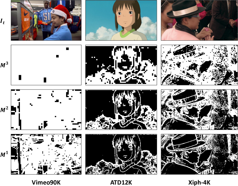
To demonstrate the superiority of sparse representation in wavelet domain for efficient frame interpolation, we explore the accuracy vs efficiency relationship by setting different fixed compression threshold ratio in the second training step, and the corresponding is also used during evaluation. We select 7 typical values of to carry out above experiments on diverse datasets, whose results are summarized in Table IV. For better intuitive understanding, we depict the relative change curves of score loss ratio against computation reduction ratio in Fig. 9, where is set to 0 in all these cases. In Fig. 9, each point stands for an experiment result of one specific value, and gradually increases from left to right in a specific line. As is expected, larger will result in less computation and lower performance, however, the relative change rate of accuracy vs efficiency shows big difference among different datasets. On Vimeo90K, PSNR drops about 0.7% when computation is reduced by 10%. While on ATD12K, PSNR only drops about 0.4% even computation is reduced by 40%. It concludes that for a fixed , relative computation reduction is more obvious when there is more sparse low frequency texture in this dataset. Fig. 10 visually supports this conclusion by showing predicted multi-scale sparse valid masks on different VFI datasets under the same compression threshold ratio . This phenomenon also appears in traditional image compression [19, 20, 21], which means that high resolution or cartoon images are more spatially redundant to achieve higher compression ratio under the same compressed image quality.
IV-D3 Dynamic Compression Threshold Ratio Selection
To verify proposed dynamic compression threshold ratio selection approach for instance-aware efficient frame interpolation, we vary computation cost regularization parameter during the second training step and record results of these dynamic models on diverse datasets, which are presented in Table VI. In this ablation, we set and threshold ratio candidates as 0.000, 0.005, 0.010 and 0.015 corresponding to above fixed threshold ratio experiments. The baseline method that does not use any wavelet compression approach is also listed in the first line for reference. In Table VI, the dynamic model tends to employ more computation to achieve better accuracy when given relatively small , which is realized by selecting relatively small by the threshold classifier during end-to-end optimization. For a more intuitive comparison between fixed and dynamic settings, we further plot their accuracy vs efficiency trade-off line charts in Fig. 12. As is depicted, under the same computation cost, the relative improvement of dynamic selection approach against fixed threshold method behaves different in regard to both and datasets.
| Dynamic | Vimeo90K | ATD12K | Xiph-2K | Xiph-4K | |||||||||
|---|---|---|---|---|---|---|---|---|---|---|---|---|---|
| TFLOPs | PSNR | SSIM | TFLOPs | PSNR | SSIM | TFLOPs | PSNR | SSIM | TFLOPs | PSNR | SSIM | ||
| ✗ | 0.0 | 0.090 | 35.71 | 0.9791 | 0.409 | 28.83 | 0.9566 | 1.746 | 36.40 | 0.9664 | 1.746 | 33.62 | 0.9453 |
| ✓ | 0.1 | 0.087 | 35.69 | 0.9789 | 0.317 | 28.83 | 0.9564 | 1.659 | 36.41 | 0.9662 | 1.650 | 33.62 | 0.9453 |
| ✓ | 0.5 | 0.084 | 35.66 | 0.9784 | 0.313 | 28.83 | 0.9564 | 1.543 | 36.37 | 0.9654 | 1.552 | 33.62 | 0.9452 |
| ✓ | 1.0 | 0.081 | 35.58 | 0.9775 | 0.274 | 28.79 | 0.9555 | 1.480 | 36.32 | 0.9650 | 1.428 | 33.61 | 0.9448 |
| ✓ | 3.0 | 0.079 | 35.41 | 0.9753 | 0.270 | 28.78 | 0.9553 | 1.393 | 36.05 | 0.9609 | 1.377 | 33.54 | 0.9436 |
| ✓ | 5.0 | 0.077 | 35.21 | 0.9730 | 0.247 | 28.74 | 0.9541 | 1.336 | 35.75 | 0.9573 | 1.274 | 33.30 | 0.9409 |
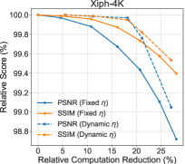
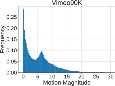
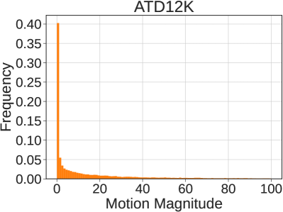
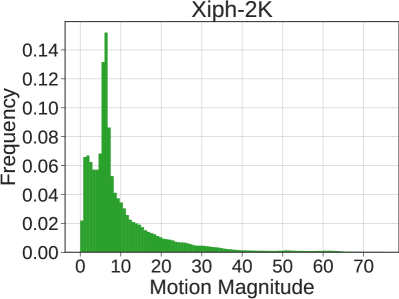
For the first factor, the relative improvement is more obvious when is set to a medium value. It is because that in this case the threshold classifier can have more chance to select different threshold candidates by learning the instance difference for frame interpolation. On the other hand, dynamic method tends to degrade to fixed method when given relatively large or small . Therefore, we employ in WaveletVFI due to its largest performance gain. As for the second factor, the relative improvement is more obvious when the variation of spatial-temporal texture distribution in this dataset is larger. To prove it, we use FastFlowNet [68] to estimate inter-frame optical flow and analyze their motion magnitude statistics, whose results are shown in Table V and Fig. 11. As can be seen in Fig. 12, there is almost no difference on ATD12K since it has relatively large motion variation but relatively small texture variation. On the other hand, the relative computation reduction under the same accuracy is much more obvious on the challenging Xiph-4K dataset. It is because that both the texture and the motion distribution variation on Xiph-4K are relatively large. In summary, proposed dynamic threshold selection approach in wavelet domain can achieve similar accuracy as the baseline method, while reducing computation cost by 10.0%, 33.0%, 15.2% and 18.2% on Vimeo90K, ATD12K, Xiph-2K and Xiph-4K benchmarks respectively.
IV-E Discussion on Dynamic Threshold Selection
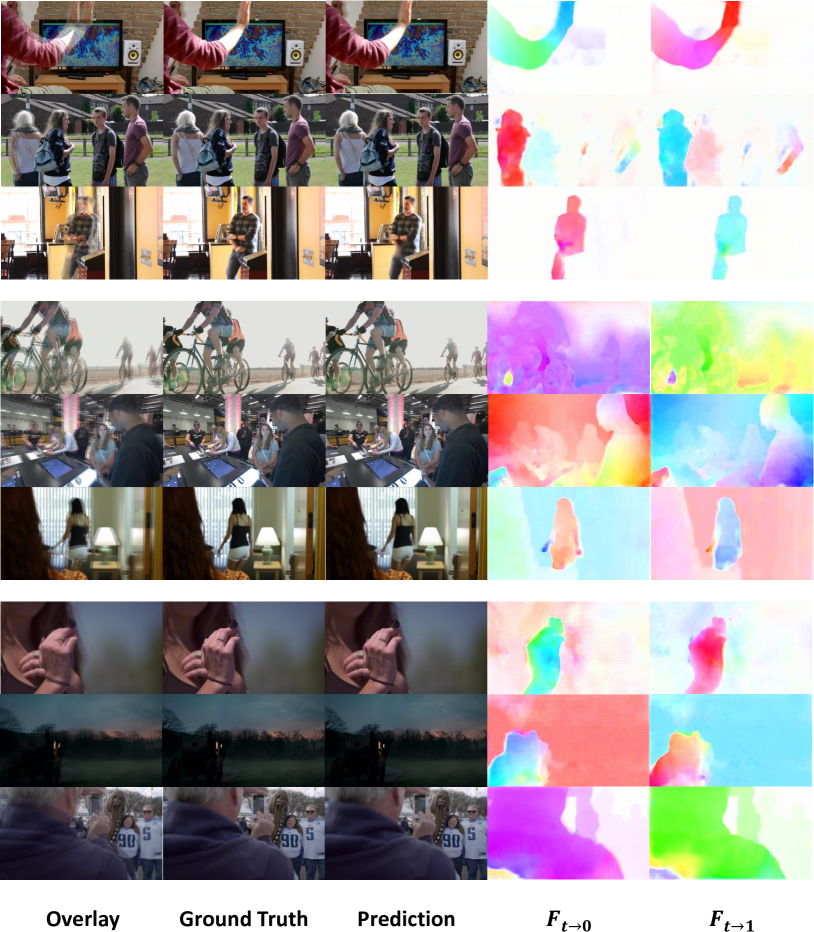
In this part, we analyze the dynamic prediction results of the compression threshold ratio classifier on Vimeo90K test set with set to 1 during the second training step. Prediction results with different threshold ratio selection are visualized in Fig. 13. Intuitively, we can get following conclusions. 1) In the top group of Fig. 13, when input frames come from rich and clear texture, and the inter-frame motion is relatively simple, the threshold classifier tends to estimate a small , that consumes more computation to synthesize more reliable high-frequency texture of the target frame. 2) In the middle group of Fig. 13, when input frames come from rich and clear texture, and the inter-frame motion is relatively complex, the threshold classifier tends to estimate a medium , that reduces some computation for to remove some unreliable high-frequency texture of the target frame. 3) In the bottom group of Fig. 13, when input frames come from simple and blurry texture, and the inter-frame motion is relatively complex, the threshold classifier tends to select a large , that consumes less computation to synthesize less unreliable high-frequency texture of the target frame.
IV-F Limitations
Currently, our framework only predicts the single middle frame, where . For interpolating multiple intermediate frames, it can work in a recursive manner, but which may lead to error accumulation. This problem can be solved to some extent by modeling multiple discrete intermediate optical flow with a temporal encoding conditional input like IFRNet [29], that can approximate arbitrary time interpolation.
V Conclusion
To our best knowledge, it is the first time that the spatial redundancy problem in frame interpolation is studied in detail, which is particularly important with the popularity of high-resolution displays. In this work, we have proposed a novel frame interpolation algorithm in wavelet domain to achieve on par accuracy with SOTA methods but with better efficiency. Our method exploits the sparse representation in wavelet decomposition and employs sparse convolution to predict multi-scale wavelet coefficients in certain critical areas for computation reduction. Moreover, we have proposed a dynamic threshold selection approach to better allocate computation for each input sample. Experiments on the traditional low resolution, current high resolution and animation frame interpolation benchmarks demonstrate the effectiveness of proposed contributions, which can significantly reduce the overall resource consumption while maintaining advanced VFI accuracy. Since our approaches are orthogonal and complements other efficient methods, such as channel pruning, we hope proposed WaveletVFI can benefit the related communities.
References
- [1] H. Jiang, D. Sun, V. Jampani, M.-H. Yang, E. Learned-Miller, and J. Kautz, “Super slomo: High quality estimation of multiple intermediate frames for video interpolation,” in 2018 IEEE/CVF Conference on Computer Vision and Pattern Recognition, 2018.
- [2] C. L. Zitnick, S. B. Kang, M. Uyttendaele, S. Winder, and R. Szeliski, “High-quality video view interpolation using a layered representation,” in ACM SIGGRAPH 2004 Papers, 2004.
- [3] L. Siyao, S. Zhao, W. Yu, W. Sun, D. Metaxas, C. C. Loy, and Z. Liu, “Deep animation video interpolation in the wild,” in Proceedings of the IEEE/CVF Conference on Computer Vision and Pattern Recognition (CVPR), 2021.
- [4] Y. Dar and A. M. Bruckstein, “Motion-compensated coding and frame rate up-conversion: Models and analysis,” IEEE Transactions on Image Processing, 2015.
- [5] S. Dikbas and Y. Altunbasak, “Novel true-motion estimation algorithm and its application to motion-compensated temporal frame interpolation,” IEEE Transactions on Image Processing, 2013.
- [6] S. Niklaus and F. Liu, “Context-aware synthesis for video frame interpolation,” in Proceedings of the IEEE Conference on Computer Vision and Pattern Recognition (CVPR), 2018.
- [7] W. Bao, W.-S. Lai, C. Ma, X. Zhang, Z. Gao, and M.-H. Yang, “Depth-aware video frame interpolation,” in 2019 IEEE/CVF Conference on Computer Vision and Pattern Recognition (CVPR), 2019.
- [8] S. Niklaus and F. Liu, “Softmax splatting for video frame interpolation,” in Proceedings of the IEEE/CVF Conference on Computer Vision and Pattern Recognition (CVPR), 2020.
- [9] X. Xu, L. Siyao, W. Sun, Q. Yin, and M.-H. Yang, “Quadratic video interpolation,” in Advances in Neural Information Processing Systems, 2019.
- [10] Y. Zhang, C. Wang, and D. Tao, “Video frame interpolation without temporal priors,” in Advances in Neural Information Processing Systems, 2020.
- [11] Z. Chi, R. Mohammadi Nasiri, Z. Liu, J. Lu, J. Tang, and K. N. Plataniotis, “All at once: Temporally adaptive multi-frame interpolation with advanced motion modeling,” in Computer Vision – ECCV 2020, 2020.
- [12] H. Sim, J. Oh, and M. Kim, “Xvfi: extreme video frame interpolation,” in Proceedings of the IEEE/CVF International Conference on Computer Vision (ICCV), 2021.
- [13] T. Xue, B. Chen, J. Wu, D. Wei, and W. T. Freeman, “Video enhancement with task-oriented flow,” International Journal of Computer Vision (IJCV), 2019.
- [14] H. Zhang, Y. Zhao, and R. Wang, “A flexible recurrent residual pyramid network for video frame interpolation,” in Computer Vision – ECCV 2020, 2020.
- [15] Z. Huang, T. Zhang, W. Heng, B. Shi, and S. Zhou, “Real-time intermediate flow estimation for video frame interpolation,” in Proceedings of the European Conference on Computer Vision (ECCV), 2022.
- [16] J. Park, K. Ko, C. Lee, and C.-S. Kim, “Bmbc: Bilateral motion estimation with bilateral cost volume for video interpolation,” in European Conference on Computer Vision, 2020.
- [17] J. Park, C. Lee, and C.-S. Kim, “Asymmetric bilateral motion estimation for video frame interpolation,” in Proceedings of the IEEE/CVF International Conference on Computer Vision (ICCV), 2021.
- [18] M. W. Marcellin, M. A. Lepley, A. Bilgin, T. J. Flohr, T. T. Chinen, and J. H. Kasner, “An overview of quantization in jpeg 2000,” Signal Processing: Image Communication, 2002.
- [19] J. Choi and B. Han, “Task-aware quantization network for jpeg image compression,” in Computer Vision – ECCV 2020, 2020.
- [20] A. Przelaskowski, “Statistical modeling and threshold selection of wavelet coefficients in lossy image coder,” in 2000 IEEE International Conference on Acoustics, Speech, and Signal Processing. Proceedings, 2000.
- [21] S. Chang, B. Yu, and M. Vetterli, “Adaptive wavelet thresholding for image denoising and compression,” IEEE Transactions on Image Processing, 2000.
- [22] C. Montgomery, “Xiph.org Video Test Media (derf’s collection), the Xiph Open Source Community,” Online, https://media.xiph.org/video/derf, 1994.
- [23] S. Niklaus, L. Mai, and F. Liu, “Video frame interpolation via adaptive convolution,” in 2017 IEEE Conference on Computer Vision and Pattern Recognition (CVPR), 2017.
- [24] ——, “Video frame interpolation via adaptive separable convolution,” in 2017 IEEE International Conference on Computer Vision (ICCV), 2017.
- [25] H. Lee, T. Kim, T.-y. Chung, D. Pak, Y. Ban, and S. Lee, “Adacof: Adaptive collaboration of flows for video frame interpolation,” in Proceedings of the IEEE/CVF Conference on Computer Vision and Pattern Recognition (CVPR), 2020.
- [26] X. Cheng and Z. Chen, “Video frame interpolation via deformable separable convolution,” in Proceedings of the AAAI Conference on Artificial Intelligence, 2020.
- [27] S. Gui, C. Wang, Q. Chen, and D. Tao, “Featureflow: Robust video interpolation via structure-to-texture generation,” in Proceedings of the IEEE/CVF Conference on Computer Vision and Pattern Recognition (CVPR), 2020.
- [28] M. Choi, H. Kim, B. Han, N. Xu, and K. M. Lee, “Channel attention is all you need for video frame interpolation,” in Proceedings of the AAAI Conference on Artificial Intelligence, 2020.
- [29] L. Kong, B. Jiang, D. Luo, W. Chu, X. Huang, Y. Tai, C. Wang, and J. Yang, “Ifrnet: Intermediate feature refine network for efficient frame interpolation,” in Proceedings of the IEEE/CVF Conference on Computer Vision and Pattern Recognition (CVPR), 2022.
- [30] J. Liu, L. Kong, and J. Yang, “Atca: an arc trajectory based model with curvature attention for video frame interpolation,” in 2022 IEEE International Conference on Image Processing (ICIP), 2022.
- [31] L. Kong, J. Liu, and J. Yang, “Progressive motion context refine network for efficient video frame interpolation,” IEEE Signal Processing Letters, 2022.
- [32] T. Ding, L. Liang, Z. Zhu, and I. Zharkov, “Cdfi: Compression-driven network design for frame interpolation,” in Proceedings of the IEEE/CVF Conference on Computer Vision and Pattern Recognition, 2021.
- [33] M. Choi, S. Lee, H. Kim, and K. M. Lee, “Motion-aware dynamic architecture for efficient frame interpolation,” in Proceedings of the IEEE/CVF International Conference on Computer Vision (ICCV), 2021.
- [34] M. Unser and T. Blu, “Mathematical properties of the jpeg2000 wavelet filters,” IEEE Transactions on Image Processing, 2003.
- [35] D. Taubman and M. Marcellin, JPEG2000 Image Compression Fundamentals, Standards and Practice. Springer Publishing Company, Incorporated, 2013.
- [36] D. Donoho, “De-noising by soft-thresholding,” IEEE Transactions on Information Theory, 1995.
- [37] L. Liu, J. Liu, S. Yuan, G. Slabaugh, A. Leonardis, W. Zhou, and Q. Tian, “Wavelet-based dual-branch network for image demoiréing,” in Computer Vision – ECCV 2020: 16th European Conference, Glasgow, UK, August 23–28, 2020, Proceedings, Part XIII, 2020.
- [38] H. Huang, R. He, Z. Sun, and T. Tan, “Wavelet-srnet: A wavelet-based cnn for multi-scale face super resolution,” in 2017 IEEE International Conference on Computer Vision (ICCV), 2017.
- [39] H. Zhang, Z. Jin, X. Tan, and X. Li, “Towards lighter and faster: Learning wavelets progressively for image super-resolution,” in Proceedings of the 28th ACM International Conference on Multimedia, 2020.
- [40] X. Deng, R. Yang, M. Xu, and P. L. Dragotti, “Wavelet domain style transfer for an effective perception-distortion tradeoff in single image super-resolution,” in 2019 IEEE/CVF International Conference on Computer Vision (ICCV), 2019.
- [41] M. Yang, F. Wu, and W. Li, “Waveletstereo: Learning wavelet coefficients of disparity map in stereo matching,” in Proceedings of the IEEE/CVF Conference on Computer Vision and Pattern Recognition (CVPR), 2020.
- [42] M. Ramamonjisoa, M. Firman, J. Watson, V. Lepetit, and D. Turmukhambetov, “Single image depth prediction with wavelet decomposition,” in Proceedings of the IEEE/CVF Conference on Computer Vision and Pattern Recognition (CVPR), 2021.
- [43] C. J. Maddison, D. Tarlow, and T. Minka, “A∗ sampling,” in Advances in Neural Information Processing Systems, 2014.
- [44] E. Jang, S. S. Gu, and B. Poole, “Categorical reparameterization with gumbel-softmax,” ArXiv, 2017.
- [45] T. Bolukbasi, J. Wang, O. Dekel, and V. Saligrama, “Adaptive neural networks for efficient inference,” in Proceedings of the 34th International Conference on Machine Learning, 2017.
- [46] G. Huang, D. Chen, T. Li, F. Wu, L. van der Maaten, and K. Q. Weinberger, “Multi-scale dense networks for resource efficient image classification,” in ICLR, 2018.
- [47] X. Wang, F. Yu, Z.-Y. Dou, T. Darrell, and J. E. Gonzalez, “Skipnet: Learning dynamic routing in convolutional networks,” in Proceedings of the European Conference on Computer Vision (ECCV), 2018.
- [48] A. Veit and S. Belongie, “Convolutional networks with adaptive inference graphs,” in Proceedings of the European Conference on Computer Vision (ECCV), 2018.
- [49] Y. Bengio, N. Léonard, and A. C. Courville, “Estimating or propagating gradients through stochastic neurons for conditional computation,” ArXiv, vol. abs/1308.3432, 2013.
- [50] E. Bengio, P.-L. Bacon, J. Pineau, and D. Precup, “Conditional computation in neural networks for faster models,” ArXiv, vol. abs/1511.06297, 2015.
- [51] J. Lin, Y. Rao, J. Lu, and J. Zhou, “Runtime neural pruning,” in Advances in Neural Information Processing Systems, 2017.
- [52] C. Li, G. Wang, B. Wang, X. Liang, Z. Li, and X. Chang, “Dynamic slimmable network,” in Proceedings of the IEEE/CVF Conference on Computer Vision and Pattern Recognition (CVPR), 2021.
- [53] S. Cao, L. Ma, W. Xiao, C. Zhang, Y. Liu, L. Zhang, L. Nie, and Z. Yang, “Seernet: Predicting convolutional neural network feature-map sparsity through low-bit quantization,” in 2019 IEEE/CVF Conference on Computer Vision and Pattern Recognition (CVPR), 2019.
- [54] S. Kong and C. Fowlkes, “Pixel-wise attentional gating for scene parsing,” in 2019 IEEE Winter Conference on Applications of Computer Vision (WACV), 2019.
- [55] T. Verelst and T. Tuytelaars, “Dynamic convolutions: Exploiting spatial sparsity for faster inference,” in Proceedings of the IEEE/CVF Conference on Computer Vision and Pattern Recognition (CVPR), 2020.
- [56] M. Ren, A. Pokrovsky, B. Yang, and R. Urtasun, “Sbnet: Sparse blocks network for fast inference,” in 2018 IEEE/CVF Conference on Computer Vision and Pattern Recognition, 2018.
- [57] D. Sun, X. Yang, M.-Y. Liu, and J. Kautz, “Pwc-net: Cnns for optical flow using pyramid, warping, and cost volume,” in 2018 IEEE/CVF Conference on Computer Vision and Pattern Recognition, 2018.
- [58] L. Kong and J. Yang, “Fdflownet: Fast optical flow estimation using a deep lightweight network,” in 2020 IEEE International Conference on Image Processing (ICIP), 2020.
- [59] L. Kong, X. Yang, and J. Yang, “Oas-net: Occlusion aware sampling network for accurate optical flow,” in ICASSP 2021 - 2021 IEEE International Conference on Acoustics, Speech and Signal Processing (ICASSP), 2021.
- [60] M. Kivanc Mihcak, I. Kozintsev, K. Ramchandran, and P. Moulin, “Low-complexity image denoising based on statistical modeling of wavelet coefficients,” IEEE Signal Processing Letters, 1999.
- [61] A. Lewis and G. Knowles, “Image compression using the 2-d wavelet transform,” IEEE Transactions on Image Processing, 1992.
- [62] X. Cheng and Z. Chen, “Multiple video frame interpolation via enhanced deformable separable convolution,” IEEE Transactions on Pattern Analysis and Machine Intelligence, 2021.
- [63] P. Charbonnier, L. Blanc-Feraud, G. Aubert, and M. Barlaud, “Two deterministic half-quadratic regularization algorithms for computed imaging,” in Proceedings of 1st International Conference on Image Processing, 1994.
- [64] S. Meister, J. Hur, and S. Roth, “UnFlow: Unsupervised learning of optical flow with a bidirectional census loss,” in Proceedings of the AAAI Conference on Artificial Intelligence, 2018.
- [65] L. Kong and J. Yang, “Mdflow: Unsupervised optical flow learning by reliable mutual knowledge distillation,” IEEE Transactions on Circuits and Systems for Video Technology, 2022.
- [66] I. Loshchilov and F. Hutter, “Decoupled weight decay regularization,” in 7th International Conference on Learning Representations, 2019.
- [67] Z. Wang, A. Bovik, H. Sheikh, and E. Simoncelli, “Image quality assessment: from error visibility to structural similarity,” IEEE Transactions on Image Processing, 2004.
- [68] L. Kong, C. Shen, and J. Yang, “Fastflownet: A lightweight network for fast optical flow estimation,” in 2021 IEEE International Conference on Robotics and Automation (ICRA), 2021.