The generation of curves and surfaces from given data is a well-known problem in Computer-Aided Design that can be approached using subdivision schemes. They are powerful tools that allow obtaining new data from the initial one by means of simple calculations. However, in some applications, the collected data are given with noise and most of schemes are not adequate to process them. In this paper, we present some new families of binary univariate linear subdivision schemes using weighted local polynomial regression. We study their properties, such as convergence, monotonicity, polynomial reproduction and approximation and denoising capabilities. For the convergence study, we develop some new theoretical results. Finally, some examples are presented to confirm the proven properties.
keywords:
Weighted-least squares method, binary linear subdivision, noisy data, convergence criteria.
††journal: J. Sci. Comput.label1label1footnotetext: This research has been supported by project CIAICO/2021/227 (funded by Conselleria de Innovación, Universidades, Ciencia y Sociedad digital, Generalitat Valenciana) and by grant PID2020-117211GB-I00 (funded by MCIN/AEI/10.13039/501100011033).
1 Introduction
In past years, many techniques have been designed and developed in order to construct curves or surfaces with some properties such as polynomial reproduction or monotonicity-preservation. For example, splines, non-uniform rational B-splines (NURBS) and others (see, e.g. [2, 8]).
In this context, linear subdivision schemes appears as useful and efficient instruments due to their simple computation (see e.g. [7, 17, 22]). They consist in obtaining new points from given data using refinement operators and can be classified depending on such operators: if a single operator is used for all the iterations, then the subdivision scheme is called stationary or level-independent (see e.g. [7, 14]), otherwise it is denominated non-stationary or level dependent (see e.g. [9, 10, 16]). They are also classified by the linearity of the operators (see e.g. [12, 13]).
There is a vast literature on the generation of subdivision schemes and the study of their properties. An essential property is convergence, which means that the process converges uniformly to a continuous function, for any initial values. Deslauriers and Dubuc, in [11], analysed that the scheme based on centered Lagrange interpolation is convergent using Fourier transform techniques to prove it.
One of the most common studied properties is the reproduction of polynomials, i.e., if the given data are point-values of a polynomial, then the subdivision scheme generates more point-values of such polynomial. This is studied in detail in [15]. Its study is interesting since the reproduction is linked with convergence properties and the approximation capability of the scheme.
In some real applications, the given data come from measures that are contaminated by noise and, as a consequence, a suitable subdivision scheme should be used to converge to an appropriate limit function. To this purpose, Dyn et al. in [14] propose a new linear scheme based on least-square methods where the noise is reduced by applying the scheme several times. These schemes are determined by two parameters and with : For each consecutive data values, , attached to some equidistant knots , a polynomial regression is performed. The search is constrained to polynomials of degree and leads to a unique solution, , that minimizes the regression error concerning the -norm (least-squares):
(1)
The subdivision refinement rules can be obtained by evaluating at a certain point, which, in this work, is assumed to be 0 without loss of generalization.
The resulting schemes are linear, which implies some benefits and drawbacks. In [14], the convergence is proved for , as well as some properties such as polynomials reproduction.
In many applied situations, the location of the data is relevant to obtain the approximation, hence a weight function is considered to assign values depending on the distance from the knots to 0. These methods, as Shepard’s algorithm (see [24]), are called moving least squares (see [20]).
In [4, 5], the weighted local polynomial regression (WLPR) was used to design a prediction operator for a multiresolution algorithm, leading to good results on image processing when the data was contaminated with some noise. Prediction operators can be considered subdivision operators and their properties can be studied [9]. In this paper, we study the family of subdivision schemes based on the prediction operators in [4] and develop a new technique to study their convergence based on some asymptotic behaviour. Also, some properties such as polynomial reproduction, the Gibbs phenomenon in discontinuous data, monotonicity preservation and denoising and approximation capabilities are analysed. We provide some examples to check the theoretical results.
The paper is organized as follows: Firstly, we briefly review the classical components of linear subdivision schemes with the aim to be self-contained in this work. In Section 3, we explain the WLPR and define a general form, leading to new subdivision schemes definitions. Afterward, we study different properties in some particular cases: Starting with , we analyse the convergence, the smoothness of the limit functions, the monotonicity preservation and the Gibbs phenomenon when the initial data present large gradients. In Section 5, we develop a new technique to study the convergence of a family of schemes and apply it to the case .
We analyse the approximation and noise reduction capabilities of the new schemes in Sections 7 and 8. Finally, some numerical experiments are performed to confirm the theoretical properties, in Section 9, and some conclusions and future work are proposed.
2 Preliminaries: A brief review of linear subdivision schemes
Let us denote by the set of bounded real sequences with indices in . A linear binary univariate subdivision operator with finitely supported mask is defined to refine the data on the level , , as:
(2)
In this work, we only consider level-independent subdivision schemes, meaning that the successive application of a unique operator constitutes the subdivision scheme. Hence, we will refer to as the subdivision scheme as well.
The binary adjective refers to the two formulas/rules of (2) (corresponding to and ) which are characterized by the even mask and the odd mask . It is called length of a mask to the number of elements that are between the first and the last non-zero elements, both included.
Remark 2.1.
If a linear subdivision scheme is applied to some data , where is a smooth function and is random data, also called noise, the result is
which implies that we can study separately the smooth and the pure noisy cases.
If we apply these rules recursively to some initial data , it is desirable that the process converges to a continuous function, in the following sense.
Definition 1.
A subdivision scheme is uniformly convergent if for any initial data , there exists a continuous function such that
Then, we denote by to the limit function generated from . We write if all the limit functions have such smoothness, , .
A usual tool for the analysis of linear schemes is the symbol, that we define as follows.
Definition 2.
The symbol of a subdivision scheme is the Laurent polynomial
We can determine if a subdivision scheme is convergent depending on the sum of the absolute values of some even and odd masks. Therefore, we use the norm of the operator .
Lemma 2.1.
The norm of , as a linear endomorphism in the space of bounded sequences, is the maximum between and :
According to the Definition 5.1 of [15], a subdivision scheme is odd-symmetric if
or even-symmetric if
In terms of the symbol, these is translated as or , respectively.
The schemes, that we will construct in this paper, are odd-symmetric, but to simplify some equations, we consider a more relaxed definition of odd-symmetry and even-symmetry.
Definition 3.
A subdivision scheme is symmetric if
for some . It is even(odd)-symmetric if is odd (even).
A useful property for a subdivision scheme is the reproduction of polynomials.
Definition 4.
A subdivision scheme reproduces111Technically, this is the definition of step-wise reproduction, which is a stronger condition, [15]. (polynomials up to degree ) if
A necessary condition for convergence is the reproduction of constants. The following lemma determines the relation between the mask, the symbol and the reproduction of the constants.
Lemma 2.2.
The following facts are equivalent:
(a)
reproduces (constant functions).
(b)
.
(c)
for some Laurent polynomial .
In such case, the scheme is well-defined and called difference scheme. If , then is convergent.
There exists a direct relationship between the symmetry of and the symmetry of its difference scheme, . We introduce it in the following result.
Lemma 2.3.
If a scheme is odd-symmetric, then its difference scheme is even-symmetric.
Proof.
It can be easily checked using the symbols.
∎
Next theorem by Dyn and Levin, [17], links the smoothness of and .
Theorem 2.4.
If the scheme based on is convergent and , then is convergent and .
Remark 2.2.
We give now a more explicit formula to compute for the kind of schemes we consider in this paper. We will analyze odd-symmetric subdivision schemes, which implies that the length of the mask is always odd and two possible situations may occur, depending on which sub-mask has the largest support.
Since the sub-masks and are finitely supported, from now on we will treat them as vectors containing only their support, which will be important for the theoretical results in Section 5.
The first situation is that, for some , the sub-masks are and , while the second one corresponds to and (pay attention to the supports).
To compute with a unique formula for both cases, we redefine the mask for the second case, consisting in , , and , . Now the first indices of the supports are , in both situations, and the last indices are and (for the first and second sub-mask, respectively) for the first situation and and for the second one. Now, in both cases, the second sub-masks is the largest and we can affirm that there exists some such that
(3)
with or , so that and . In any case, now the odd-symmetry is written as
Finally, for a subdivision operator written as (3), the difference mask can be computed as follows:
(4)
According to Lemma 2.3, is an even-symmetric scheme. In particular,
(5)
3 Weighted local polynomial regression (WLPR)
The schemes analysed in the present work has been applied to image processing in a multiresolution context as prediction operator both for point-values as for cell-average discretizations, (see, e.g. [4, 5]). They are based on weighted local polynomial regression (WLPR) and they can be defined by inserting a weight function in the minimization problem (1),
which emphasizes the points closer to where the new data is attached.
In this section, we briefly introduce WLPR and describe some of its properties. For a more detailed description, see [19, 21].
Firstly, we fix the space of functions where the regression is performed: , the space of polynomials of degree at most . Other function spaces could be used as well (see [19]). We can parametrize the polynomials in as
where the superscript is the matrix transposition, and . The vectors are considered column vectors in order to perform the matrix multiplication. With this notation, the regression problem (1) can be expressed as
(6)
The second ingredient is the weight function, , which assigns a value to the distance between and 0, which is the location where is evaluated in this work. We define as
and we impose that is a decreasing function such that .
With these assumptions it is clear that has compact support, , is even, increasing in and decreasing in , and it reaches the maximum at point . The choice assigns the highest weight to the point where is evaluated. In [21], some functions are proposed, which we compile in Table 1. Observe that many of them have the form with .
The parameter determines how many data values are used in the regression and allows to distribute the weights of the points used in the rank .
By the properties of the function , if , then for any .
Finally, we choose a vector norm, typically is taken for its simplicity, but any -norm can be used depending on the characteristics of the problem. The loss function is defined accordingly: .
With the above elements, we propose these two problems to design the two subdivision rules:
(8)
Once the fitted polynomial is obtained, it is evaluated at 0 to define the new data:
(9)
so that only the first coordinate of is needed.
Proposition 3.1.
Moreover, for , the resulting subdivision scheme is the Deslauriers-Dubuc subdivision scheme.
Proof.
Let us discuss when this scheme is well defined. Two situations may occur, depending on whether or not (the polynomial degree) is smaller than the amount of data in the minimization problem (8).
For , if
then (8) is a least square problem and there is a unique solution [6], otherwise it can be found a polynomial that interpolates the data. Even if the interpolating polynomial is not unique, its evaluation at 0 is exactly . Hence, the even rule is well defined for any , coinciding with the even rule of the Deslauriers-Dubuc subdivision scheme for , i.e. .
For , a least of square problem is solved if
and an interpolation problem with unique solution is solved when the equality is reached, coinciding with the Deslaurier-Dubuc odd rule in the last case. However, nor the polynomial neither its value at zero are unique when , so that the scheme is not well defined in this case.
As conclusion, only if the polynomial degree is , the resulting scheme is the Deslauriers-Dubuc interpolatory subdivision scheme, independently the choice of and the loss function .
∎
The scheme (9) coincides with the proposed by Dyn et al. in [14] if and are used (corresponding to rect in Table 1). Also, the non-linear subdivision scheme presented by Mustafa et al. in [23] can be obtained with the same choice of but with .
We will analyse the properties of our schemes specifically for the polynomial degrees , the loss function and several choices of .
We will study how the choice of affects the approximation and noise reduction capabilities. We will show that it is not possible to define a giving the best approximation and the greatest denoising. In fact, one may decide how much importance to adjudge to each property and find an equilibrium. This decision may be based on the magnitude of the noise and the smoothness of the underlying function.
Observe that, when , for some , the even rule () support is shorter than the odd () one, and just the opposite occurs when . To simplify, we will discuss in detail the first case, where even and odd masks have lengths and , respectively, since the second one is analogue and the Remark 2.2 can be taken into account for the consequent analysis. Nevertheless, we deal with both situations along the paper when it can be do it without additional effort.
To give a more explicit definition of the schemes, we solve the quadratic problem posed in (8) with . In this case, it is a weighted least square problem and its solution is well-known.
Let us start with the derivation of the odd sub-mask, , for .
For the sake of simplicity, we omit the dependence on for the following vectors and matrices. If we denote as the diagonal matrix consisting on the vector
(10)
we call
(11)
where the powers , , are computed component-wisely, so that is a matrix,
and we denote , then the problem of
(8)
can be write as:
(12)
whose solution is
(13)
For the sake of clarity, we write down the above terms:
(14)
and
Since we only need the first coordinate , we can use the Cramer’s formula instead of solving the full system:
Observe that, since the vector is symmetric, , then for any odd value of , and for the even values.
Thus, the above expressions can be simplified by placing many zeros and by shorting the range of the remaining sums.
Using the linearity of the determinant respect to the first column,
we conclude that the sub-masks coefficients are
By (13), it can also be expressed as , where is the first element of the canonical basis of .
Analogously, for , we can prove that , so that
where
is the diagonal matrix with diagonal
(15)
and
Collecting these developments, for , we can define our weighted local polynomial regression-based subdivision as:
(16)
A direct consequence, by construction, is that the scheme reproduces polynomials up to degree .
Proposition 3.2.
The scheme reproduces .
Remark 3.1.
Observe that we have considered as basis of , which has led a the linear system with matrix (14). It is possible to consider an orthonormal basis of in a way that the matrix is diagonal, leading to a cleaner mathematical description. However, we preferred the basis because the resulting expression of the subdivision operator is more explicit. A possible benefit of considering an orthonormal basis is that the next results might be more intuitive.
Now we prove that , , are exactly the evaluations of some polynomial at the grid points .
Lemma 3.3.
For , the sub-masks are
(17)
That is,
the vector coincides with the evaluation of the polynomial at the points , being , which expression depends on .
That is, the coordinates of are the evaluations of the polynomial at the grid points.
∎
Moreover, these sub-masks are the only ones that lead to polynomial reproduction and verify that are polynomial evaluations. This property can be used in practice to easily determine the sub-masks, as we do in Section 6.
Theorem 3.4.
The scheme is the unique scheme that reproduces polynomials and its sub-masks have the form , for some , .
Proof.
It is a consequence of Lemma 3.3 together with Proposition 3.2. Suppose that some rule , for some , fulfils the reproduction conditions for . Then
or, written with matrix multiplications,
Then,
∎
The symmetry of the scheme is another consequence of being based on a polynomial regression problem.
Lemma 3.5.
The scheme is odd-symmetric.
Proof.
We prove that for (it can be analogously proven that for ). Let us consider .
The coordinates of the sub-mask can be obtained by applying the rule to , for , and take the first coordinate,
Then, provided that , or in other words, .
Observe that,
and, performing the change in the summation index by and using and ,
(19)
Observe the similarity between (18) and (19). Since the minimum is unique, it is reached in (19) by . Thus and, then, .
∎
By Lemma 3.3, we know that are the evaluations of a polynomial at . To take profit of the symmetry, let us write as in (17):
(20)
Since , , and , , and is even, it can be deduced that the polynomials only have even powers. That is
(21)
A direct consequence is that the subdivision schemes obtained for any weight function of degree (even number) coincides with the one for , proven in the following lemma.
Proposition 3.6.
Let a weight function, and be such that ,
then
Proof.
The sub-masks of can be written in terms of the evaluation of a -degree polynomial, according to Lemma 3.3. Since the odd coefficients are zero, then the leading coefficient is zero, for both rules . Then, both and fulfils the conditions of Theorem 3.4, for the same polynomial degree , hence they must coincide. ∎
Therefore, we can just study the properties of the subdivision schemes based on the space of polynomials with an even number.
4 WLPR-Subdivision schemes for
In this section we present the WLPR-Subdivision schemes for and their properties, by Proposition 3.6, we can just consider . To simplify the notation, in this section we omit , and in some variables, such as . In this case, the coefficients of the subdivision schemes are easily obtained from thanks to Lemma 3.3: If we denote as
the sum of the components of the vector with , defined in (15) and (10),
(22)
thus .
Another way to obtain is based on Theorem 3.4: Since and the scheme must reproduce (constant functions), then by Lemma 2.2, thus .
The explicit form of the resulting WLPR-subdivision scheme is, if ,
(23)
and, for , it can be written in the following way, in agreement with Remark 2.2,
(24)
Note that if then and , so that the mask for any function of the subdivision scheme is , in other words, the interpolatory Deslauriers-Dubuc scheme [11] (as stated in Proposition 3.1).
For , if for , then the schemes presented by Dyn et al. in [14] are recovered as we mentioned above. These schemes are for :
(25)
We list some masks for the weight function , , and for several values of :
As we can see, all subdivision schemes in this section present a positive mask, since is a positive function. Then, the following result on convergence proved in [18], (see also [22, 26]) can be applied.
Proposition 4.1.
([18])
Let be a mask with support , being and fixed integers, . Suppose that and
then the subdivision scheme converges.
As a direct consequence, the schemes in this section,
(23) and (24), are convergent because the masks are positive. Observe that the condition in Proposition 4.1 requires considering .
Corollary 4.2.
The subdivision scheme , defined in
(23) or (24), is convergent for any and any positive function with support .
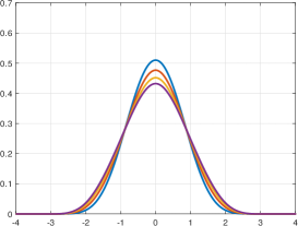
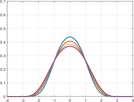
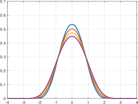
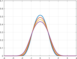
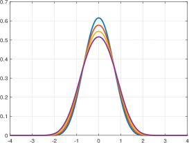
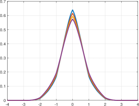
In Figure 1 we show some examples of the limit functions for some weight functions, and . The support of all these limit functions is because the mask support length does not vary.
tria
epan
bisq
tcub
trwt
exp(3)
Figure 1: Limit functions of the subdivision schemes for some weight functions (see Table 1) and (blue), (orange), (yellow) and (purple).
To analyse the smoothness of the limit functions generated by , we consider the Theorem 2.4.
In particular, we will prove that the mask of the difference scheme is positive and apply again Proposition 4.1.
Thanks to the odd-symmetry of the scheme, the study can be reduced to a half of its coefficients.
Lemma 4.3.
Let be a natural number, , and a weight function. The coefficients of the difference scheme are positive if
Proof.
By Lemma 2.3, is even-symmetric. Since , then in (5) and we have
(26)
Then, if , for , and , for , the result is proved.
First, we check that the coefficients and are always positive.
which is an increasing function since is decreasing. We have that
Again, using the same strategy, we get:
Then, by Lemma 4.3, we conclude that the coefficients of the difference scheme, (4), are positive.
∎
Next lemma allows to easily check the monotonicity of .
Lemma 4.5.
Let and be.
If is continuous and differentiable in and the quotient function is decreasing, then is decreasing.
Proof.
By hypothesis, the function is continuous for and differentiable in (observe that we are considering a real number here). Hence, it is decreasing provided that its derivative is negative. In addition,
and is decreasing by hypothesis.
∎
Table 2: Functions , and its derivative, being the functions presented in Table 1 and .
Therefore, we prove the following corollary.
Corollary 4.6( limit functions).
Let , and be. The scheme is for and for any weight function with and .
Proof.
From Table 2, the function is decreasing for any with and . Then, by Lemma 4.3 the coefficients of the difference scheme are positive and by Proposition 4.1 the subdivision scheme is convergent. The case is studied in [14].
∎
In order to finish this section, we study two properties. Firstly, we analyse if the new family of schemes conserves monotonicity. In our case, the result presented by Yad-Shalom in [25] can be used:
Proposition 4.7.
Let be a convergent subdivision scheme and its corresponding difference scheme with a positive mask. If the initial data, , is non-decreasing then the limit function is non-decreasing.
With this proposition, we can enunciate the following corollary.
Corollary 4.8(Monotonicity preservation).
For and any weight function introduced in Table 1, the scheme conserves the monotonicity.
Finally, when the initial data presents an isolated discontinuity and a linear subdivision scheme is applied several times some non-desirable effects may appear near the discontinuity, some kind of Gibbs phenomenon (see e.g. [1]).
In [1] it is proved that if the mask of the scheme is non-negative then the Gibbs phenomenon does not appear in the limit function.
Corollary 4.9(Avoiding Gibbs phenomenon).
For , the scheme avoids the Gibbs phenomenon.
In Section 9, we present some examples checking these theoretical results. For , the resulting mask is positive and we have used classic tools to study its properties. However, for , the mask are no longer positive. In the next section, we will develop a novel technique based on numerical integration for this goal and we will apply it to prove the convergence of the schemes based on weighted-least squares.
5 A tool for the convergence analysis
The purpose of this section is to provide new theoretical results to analyse the convergence. In Section 4, the convergence was easily proven by the positivity of the mask. However, in Section 6 we will prove the convergence of the scheme based on the regression with polynomials of degrees , which are no longer positive, so that we cannot follow the same strategy. Nevertheless, as a consequence of Lemma 3.3, the sub-masks can be seen as the evaluation of a second degree polynomial and this fact is advantageous and we will take profit of it in this section.
For any particular value of , a fixed and considering some such that , , it can be easily computed the difference scheme using the formula (4) and checked if its norm is less than 1, which would imply convergence. Let us call this method the direct inspection. But it serves to prove convergence only for the chosen , and we wish to prove it for all . Our strategy will consist in proving converge asymptotically, that is, to prove convergence for , for some , and then check the converge for each by direct inspection.
First, we would like to give a general idea about this asymptotic convergence. Thanks to the properties of the space of polynomials , the problem (8) can be formulated using equidistant knots in the interval , such as
(36)
The last sum is, in fact, a composite integration rule. So that, if , then and the problem seems (this is not a rigorous argument, but it serves to understand the situation) to converge to
(37)
for both . On the one hand, the given data is now a function which is approximated by a polynomial in the norm with a weight function .
On the other hand, by Lemma 3.3 the corresponding subdivision sub-masks, say , fulfils , for some coefficients . Then, the sub-masks also seem to converge to some continuos function, if some normalization is performed since the sub-masks supports increase with (see later Remark 5.1 and Section 6 for more details). The results presented in this section exploit this kind of situations.
From now on, we consider a family of subdivision schemes as in (3).
The results in this section allow to prove convergence for , for some , and also provides the value of , so that it can be checked convergence for by direct inspection. Combining both proofs, we obtain convergence for all .
In particular, will be computed, which ensures the asymptotic convergence when that limit is less than 1. Here we denote by the sub-masks of the masks .
Theorem 5.1.
Let be a sequence of subdivision schemes that reproduces , which odd rules are longer than (or as long as) the even rules, as in (3).
Let be a function and let be.
If
(38)
(39)
(40)
for some , , then the first sub-masks of the difference schemes fulfil
Now, if , we use that and the composite (forward) rectangle rule, thus obtaining that
where is the integration error of ,
If , we use the composite (backward) rectangle rule and we obtain a similar result:
Using all the upper bounds we found, we obtain:
(43)
From here we deduce that, if , then
the limit when of the right part of (43) is , which is less than 1. Hence, there exists such that , .
In particular, for , we can find for which value of the right part of (43) is equal to 1, by solving a second degree equation, arriving to (42).
∎
Remark 5.1.
In practice, if the expressions of are well defined for any (this is the case of , see (50)), then a practical way to compute is
In Section 6, a complete example of the application of the results of this section will be performed.
A similar condition will be derived from the last result to ensure that . First, we prove a result that will be useful for symmetric subdivision operators.
Theorem 5.2.
Let be as in (3) and consider a flipped version of them, , defined as
Then
Moreover, fulfil the conditions of Theorem 5.1 if, and only if, fulfil
(44)
(45)
(46)
where , and .
Proof.
Observe that
so that, defining , , the equivalence between (38)-(39) and (44)-(45) is clear.
Then
and
thus, the equivalence between (40) and (46) also holds true.
On the other hand, reproduces if, and only if, does. Hence, the finite difference scheme exists and can be computed with the formula (4).
Hence,
Since and , we deduce that the formula to compute , (42), can be used here as well.
∎
The next result is a direct consequence of the previous one.
Corollary 5.3.
Let be, as in (3), that reproduce . Let be a function and let be.
If
By the Theorem 5.2, the flipped version of this scheme fulfils Theorem 5.1 and the claimed inequality is true.
∎
For odd-symmetric subdivision operators, due to Theorem 5.2, the satisfaction of the hypothesis of Theorem 5.1 or Corollary 5.3 is sufficient to ensure convergence.
Theorem 5.4.
Let be a set of odd-symmetric subdivision schemes fulfilling the hypothesis of Theorem 5.1. Then, the subdivision scheme is convergent if with as in (42).
6 WLPR-Subdivision schemes for
We consider such that , then . The following computations could be done for as well.
First, we compute the coefficients of (denote it by from now on).
According to Lemma 3.3, the sub-masks are , , where . Then, to compute we may solve the system
We start with . Using (14) and the symmetry of and ,
Hence, using the Kramer’s formula, the three coefficients of are:
We first prove convergence in the simplest case, , in order to be used to the new convergence analysis tools, and later we discuss the general case.
6.1 Convergence of the subdivision schemes based on weighted least squares with and
In this case, , , so that the mask coefficients can be simplified to
(50)
It can be easily checked that these operators are odd-symmetric, which for sure we knew by Lemma 3.5. Hence, to prove convergence we can apply Theorem 5.4.
Observe that the algebraic expressions of and are well defined even for . Then, for any , we define
that we obtained with the aid of a symbolic computation program. We also computed that
(51)
where
Now we should find such that for . On the one hand,
On the other hand, the numerator of (51) can be easily bounded using that and increasing to 6 the degree of every monomial:
It is desirable to prove convergence for as much values of as possible, so should be chosen such that is as small as possible, but greater or equal than , due to (52). We computationally found that the compromise is achieved for , leading to . Hence, according to Theorem 5.4, the subdivision schemes are convergent for . For smaller values of , we have computationally checked that
This symbolic computation is quick and without rounding errors, so this can be considered a rigorous proof of the convergence.
We can perform some additional computations in order to provide an upper bound of valid for any .
According to (43),
We checked that the right side is less than for any , and we explicitly computed that for , . As conclusion,
and the equality is reached only for .
We tried to prove regularity with this technique by applying the results to the divided difference schemes, , but they do not satisfy (38).
6.2 Convergence of the subdivision schemes based on weighted least squares with and a general function
In this situation, we will study the convergence only for large values, so that we will not calculate , because we have not been able to perform the direct inspection without specifying .
In order to compute
we will define a function such that , ,
which will allow to write
For that purpose, we define , , .
Recall that , and . Observe that the sub-masks (48) and (49) can be expressed as
Thus, we may define the link function as
Observe that provided that ( may not exist at 0 or 1).
To follow more easily the next computations, we write , where are the numerator and denominator that appear in the last formula.
Taking into account that
we proceed to compute the derivative.
where
Finally, we proceed to compute
To this purpose, we define
(53)
we observe and we use the following composite integration rule
Defining , so that , we note that
and
so that
Taking these comments into account and taking , we find out that
Hence,
Clearly, the former expression is valid provided that . Fortunately, we can use the Schwartz’s inequality for the inner product to deduced that
We gather in Table 3 the computation of and for several choices of . Since for all of them, we conclude that, for large enough, any of the corresponding subdivision schemes converge. We realized that the value of could be greater than one for some extreme choices of . An example is , but thus kind of functions were discarded in Section 3 due to its practical meaning.
Table 3: The function and the value of Theorem 5.1 for several choices of and .
The next two sections are devoted to study the approximation and the noise suppression capability depending on the chosen weight function
7 Approximation capability
To study the approximation capability, we consider the subdivision scheme defined in (9) with and satisfying the conditions requested in Proposition 3.1. Let be and consider the initial data with and
Let be any integer, we calculate the approximation error between and , with , and analyse the largest contribution term.
By Taylor’s theorem, we have that there exist such that:
Applying the subdivision operator and considering its polynomial reproduction capability,
(54)
Therefore, the largest contribution to the approximation error is given by
We conclude that if two linear schemes are given, with the same approximation order, then the scheme with lesser value of
(55)
provides better approximators, in general. We observe that, if , for some function , , (in that case, ), then
Since the proposed schemes are odd-symmetric, then and and the approximation error is given by
(56)
which increases with and . We will test this formula in Section 9.2.
Now, we explore how the selection of influences , with the aim of determining which is the best from an approximation point of view.
For , it is easy to compute from the expression of in (23) and (24). For instance, for ,
Hence, . In Table 4, we see that the smallest values are reached for with large and for with large or small . We add for comparison , that according to Section 8, the smaller it is, the greater is its noise reduction capability. We can see for any scheme that the greater is the approximation capability, the smaller is the noise reduction capability. As conclusion, approximation and noise reduction are incompatible, in this sense, and some equilibrium may be found. This is further discussed in Section 8.1.
Then, . The same conclusion can be obtain as in the case from Table 5: The smallest values are reached for with large and for with large or small . A great approximation power implies a low noise reduction capability, which will be studied in Section 8.1.
8 Noise reduction
In this section, we study the application of a subdivision operator to purely noisy data, where all the values follows a random distribution , and are mutually uncorrelated. The results of this study can be applied to any data contaminated with noise due to Remark 2.1.
A direct result is that
Since for any convergent schemes, the best condition is reached for , for which , since the mask is positive. Hence, it cannot be concluded from this formula that the noise is reduced.
Table 4: Computations of , and for several choices of , .
Table 5: Computations of , and for several choices of , .
To reveal the denoising capabilities, a basic statistical analysis can be carried out. If the variance of the refined data is lesser than the variance of the given data, , it indicates a reduction of randomness. Using that
provided that are two uncorrelated random distributions, the variance after one subdivision step is
Hence, the variance reduction is given by
For some schemes studied in this work, this quantity is: For , if ,
The last quantity is less than one owned to the constant reproduction and the positivity of the coefficients.
In case that , then , which is the lowest value that can be obtained with a rule of this length. For , and ,
which maximum is achieved for (i.e. , corresponding to the interpolatory DD4 scheme), which is 1.
Two results can be derived: First, if the variance is reduced in each iteration by a factor , then the limit function has variance 0. Second, since , the noise tends to be completely remove when the mask support tends to .
For any choice of , an asymptotic result can be given for the noise reduction using an argument similar to Section 7: If , for some function , , then
so that the noise reduction factor behaves asymptotically as
(57)
Under these assumptions, we observe that the noise is always removed after an iteration when .
In the Tables 4 and 5 we compute and the factor for several functions, .
8.1 An equilibrium between approximating and denoising
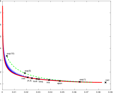
We have seen that, in order to maximize the approximation and denoising capabilities, the values and should be minimized. This is a multi-objective minimization problem, which solutions form a Pareto front that we have estimated using the MATLAB optimization toolbox. Here we will only consider the case , but a similar analysis can be performed with .
First, observe Figure 2-left. We find out that is always more convenient than , meaning that for each value of there exists some pair for which approximates and denoises better than .
It can also be affirm that is in the Pareto front and it the best for noise reduction and the worst for approximating. In the other extreme would be an interpolatory scheme, with the best approximation capability but the worst denoising power.
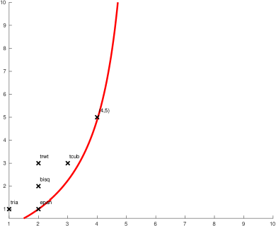
The Pareto-optimal values for form a curve (see Figure 2-right) which seems to interpolate the integer values and .
Figure 2: Left, the pair of values for several choices of . Thus, the lower and axis values, the better approximation and denoising capabilities, respectively. Blue, for several values pairs such that , ; red, the Pareto front of the previous pairs; green, for . Right, the red line represents the pairs of values () for which is Pareto-optimal.
In conclusion, we recommend the use of rect to obtain the best denoising. However, with epan the noise increases by while the approximation error is reduced by compared to rect. If the approximation is desired to be prioritized, is a good choice, since the noise increases by while the approximation error is reduced by , compared to rect. The rest of the values related to Table 1 are near to be optimal and can be used as well for other approximating-denoising balances. We recommend to never use exp().
Just to mention that for similar conclusions can be obtained. For that polynomial degrees, the weight functions are also worse than . The weight function epan is still Pareto optimal, but the pair is not.
9 Numerical experiments
In this section, we present some numerical examples to show how the new schemes work for the generation of curves. We check that the subdivision schemes are convergent for and that the curve present smoothness (but not , meaning that kinks can be produced). We analysed the approximating and denoising capabilities to numerically validate the results in Sections 7 and 8. Only for , we test the conservation of the monotonicity applying the schemes to fit a non-decreasing initial data. Finally, we perform a numerical test using the discretization of a discontinuous function and observe that the proposed methods avoid Gibbs phenomenon in the neighbourhood of an isolated discontinuity for .
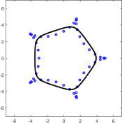
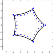
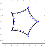
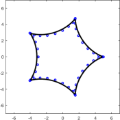
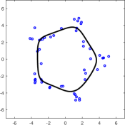
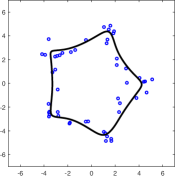
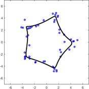
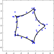
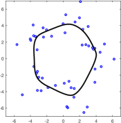
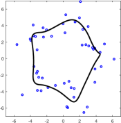
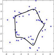
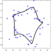
Figure 3: Several subdivision schemes (by columns) applied to the star-shaped data in
(58). In the first row, they are applied to the original data. In the second and third row, the data is contaminated by normal noise with and , respectively.
9.1 Application to noisy geometric data
We start with one of the experiments presented in [14] which consists of a star-shaped curve given by:
(58)
with samples taken at with . That is, we consider , , i.e. . Because of the periodicity of the function, we can focus on . We add Gaussian noise in each component, defining with , being , and .
In Figure 3, we illustrate the results only for two interesting choices of , according to the conclusions in Section 8.1. Nevertheless, the results obtained with the rest of weight functions are graphically similar and they are shown in detail in Table 6.
Without noise, the smaller is the more accurate are the results for any and . Measuring the approximation error as
where , . As expected, we can see in Table 6 that the approximation error is always smaller for than . But also, if we sort the weight function by the approximation order, for any , they would be exactly in the same order as if we sort them by the theoretical approximation power in Tables 4 and 5.
Nevertheless, it has to be taken into account that the results in Tables 4 and 5 have an asymptotic nature, when .
These behaviours are also visible in the first row of Figure 3.
We measure the noise reduction capability of the schemes with the quantities and , in Table 6. The ones that show results closer to zero are the schemes with higher denoising capacity. In general, the noise is more reduced when is larger or is smaller. Comparing the sorting of the weight functions by its theoretical denoising capability, according to Tables 4 and 5, and by the numbers in Table 6, we see that both orderings are the same, in general. Only in some particular cases this ordering is slightly changed. The reason may be that the results on Tables 4 and 5 are asymptotical, for . But also, the reduction is in terms of the variance of the statistical distribution. Hence, the same experiment should be repeated many times and the results averaged in order to obtain a more consistent comparison.
In Figure 3, we can see how important the choice of the weight function is to increase the approximation capability (and only losing a bit of denoising capability). In turn, taking gives better approximations and can also be increased to reduce noise.
Of course, during our study we generated much more graphics than the ones here presented. In some of them, specially in presence of noise, artefacts may appear, such as auto-intersections or kinks, proving that it does not provide curves, even if the scheme is . By taking larger, the artefacts usually disappear and curves become softer.
3.7
5.8
9.5
15.5
3.7
5.8
9.5
15.5
rect
rect
1.943e-1
4.578e-1
1.095e-0
1.844e-0
1.487e-3
1.038e-2
9.402e-2
4.899e-1
7.496e-1
5.256e-1
3.272e-1
2.506e-1
1.459e-0
9.363e-1
7.312e-1
4.073e-1
1.263e-0
9.790e-1
6.786e-1
4.712e-1
3.143e-0
1.691e-0
1.151e-0
9.408e-1
tria
tria
1.158e-1
2.695e-1
6.393e-1
1.254e-0
1.487e-3
6.683e-3
4.927e-2
2.624e-1
7.604e-1
6.518e-1
4.235e-1
2.859e-1
1.459e-0
9.048e-1
8.035e-1
5.298e-1
1.514e-0
1.170e-0
8.941e-1
6.159e-1
3.143e-0
1.957e-0
1.327e-0
1.086e-0
bisq
bisq
1.012e-1
2.363e-1
5.648e-1
1.152e-0
1.487e-3
5.986e-3
3.876e-2
2.157e-1
7.785e-1
6.816e-1
4.603e-1
2.957e-1
1.459e-0
9.140e-1
8.382e-1
5.642e-1
1.580e-0
1.209e-0
9.301e-1
6.546e-1
3.143e-0
1.959e-0
1.379e-0
1.101e-0
trwt
trwt
7.892e-2
1.859e-1
4.551e-1
9.729e-1
1.487e-3
4.134e-3
2.725e-2
1.575e-1
8.353e-1
7.111e-1
5.256e-1
3.068e-1
1.459e-0
9.860e-1
8.553e-1
6.289e-1
1.794e-0
1.290e-0
1.002e-0
7.340e-1
3.143e-0
2.128e-0
1.440e-0
1.130e-0
epan
epan
1.402e-1
3.209e-1
7.481e-1
1.416e-0
1.487e-3
8.265e-3
6.033e-2
3.161e-1
7.497e-1
6.224e-1
3.738e-1
2.832e-1
1.459e-0
9.054e-1
7.975e-1
4.861e-1
1.395e-0
1.113e-0
8.341e-1
5.575e-1
3.143e-0
1.798e-0
1.279e-0
1.051e-0
tcub
tcub
1.010e-1
2.382e-1
5.716e-1
1.171e-0
1.487e-3
5.726e-3
3.656e-2
2.072e-1
7.787e-1
6.872e-1
4.554e-1
3.023e-1
1.459e-0
9.214e-1
8.547e-1
5.677e-1
1.547e-0
1.203e-0
9.221e-1
6.453e-1
3.143e-0
1.935e-0
1.391e-0
1.104e-0
p4q5
p4q5
9.509e-2
2.286e-1
5.533e-1
1.147e-0
1.487e-3
4.666e-3
3.188e-2
1.840e-1
7.928e-1
6.993e-1
4.649e-1
3.080e-1
1.459e-0
9.606e-1
8.729e-1
5.885e-1
1.569e-0
1.214e-0
9.299e-1
6.542e-1
3.143e-0
1.984e-0
1.413e-0
1.118e-0
Table 6: Analysis of the approximation and denoising capabilities for the different subdivision schemes with
and and 15.5.
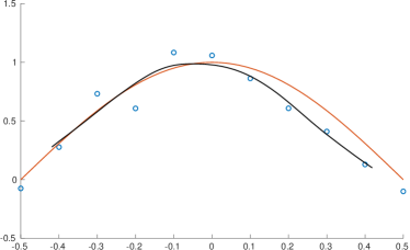
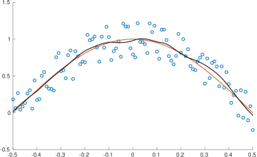
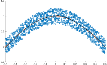
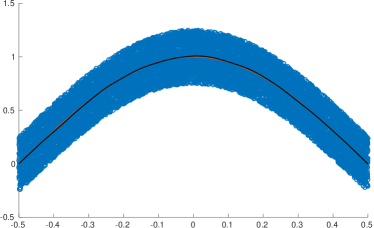
9.2 Approximation error when is being increased
In this section we challenge formula (56) with a suited experiment.
Let us consider and the initial data and with
where is the uniform distribution in the interval . We consider the spacings and the support parameters , . The value is modified accordingly to to maintain almost constant the support of the basic limit function, which determines the influence of each data point on the limit function.
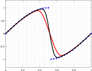
The results of applying 5 iterations of the scheme to , for , are shown in Figure 4. On the one hand, it shows how the noise after five iterations tends to 0 if , but slowly, since the variance decay speed is . On the other hand, the approximation error does not decay to zero, as can be observed in Table 7, where the numbers are never smaller than (and seems to tend to) the asymptotic error estimation in (56), which is (for , )
This threshold is not a real constrain in practice, since the noise is usually greater than the approximation error (see first row of Table 7). If an approximation error tending to zero is needed, can be chosen, for instance.
4.8215e-2
2.3619e-2
8.8646e-3
1.9704e-4
5.9734e-3
9.6240e-5
4.1201e-5
3.7387e-5
Table 7: The approximation error at after five iterations of applied to data with and without noise.
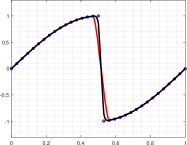
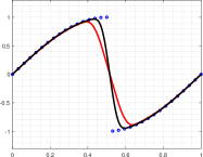
Figure 4: Five iterations of applied to , for . The blue circles are the initial data, the red line is the smooth function and the black line represents the limit function. The parameters for each graphic are (by rows): , ; , ; , ; , .
9.3 Avoiding Gibbs phenomenon
In this section we confirm that the subdivision schemes based on weighted-least squares with avoid Gibbs phenomenon, as stated in Corollary 4.9. To study it, we propose the following experiment. We discretize the function:
(59)
in the interval with 33 equidistant points, , and and apply the subdivision schemes. We show the results in Figure 5. It is clearly visualize that the Gibbs phenomenon does not appear around the discontinuity, but there is diffusion, instead. The larger is , the more diffusion, specially when rect is used.
Figure 5: Limit curves for discontinuous data using subdivision schemes with rect (red line) and trwt (black line) weight functions, .
9.4 Monotonicity
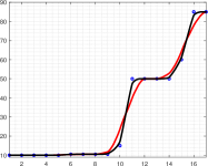
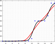
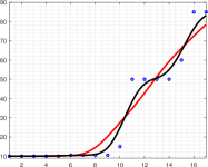
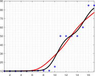
Finally, we introduce the last example in order to see numerically that the new family of the schemes conserves the monotonicity of the data, for , proved in Corollary 4.8. We apply and to the data collected in Table 8 (see [3]) and obtain Figure 6.
1
2
3
4
5
6
7
8
9
10
11
12
13
14
15
16
17
10
10
10
10
10
10.5
10.5
10.5
10.5
15
50
50
50
50
60
85
85
Table 8: Staircase data.
Figure 6: Limit curves for monotone data using subdivision schemes with rect (red line) and trwt (black line) weight functions, .
10 Conclusions and future work
In this work, a family of subdivision schemes based on weighted local polynomial regression has been analysed. We introduced the general form of this type of schemes and prove that the schemes corresponding to the polynomial degrees and coincide, for In particular, we analysed in detail the cases with positive weight functions, , with compact support.
In the first part of the paper, for , we took advantage of the positivity of the mask to prove the convergence. Also, under some conditions of the functions, the regularity of the limit function was demonstrated. Afterward, some properties were proved as monotonicity and elimination of the Gibbs phenomenon effect.
In the second part, we developed a general technique to analyse the convergence of a family of linear schemes and used it in the case .
The last sections have been dedicated to discussing noise removal and approximation capabilities. We showed how the weight function determines these properties and that it is not possible to find a maximizing both capabilities approximation and noise reduction. This led to a multi-objective optimization problem in which optimal solutions were found along a Pareto front.
Some numerical tests were presented to confirm the theoretical results.
For future works, we can consider the following ideas: The regularity of the cases were not proven. New theoretical tools such as those presented in Section 5 and their application to these schemes can be done.
We considered several weight functions from the literature. Now that we know the influence of in the approximation and denoising capabilities, it could be designed trying to improve them. Taking into account that the noise contribution is usually greater than the approximation error on the final curve, the use of an optimized weight function can be even more interesting than augmenting the polynomial degree, since some properties related to the monotonicity and the Gibbs phenomenon are only available for .
If the data present some outliers, a different loss function can provide better results. Mustafa et al. in [23] proposed a variation of Dyn’s schemes changing the -norm by the -norm in the polynomial regression but they do not prove their properties. The theoretical study of this scheme, as well as the use of different weight functions, can be considered in the future.
11 Declarations
Conflict of interest
The authors declare that they have no conflict of interest.
Data Availability Statements
Data sharing not applicable to this article as no datasets were generated or analysed during the current study.
References
[1]S. Amat, J. Ruiz, J. C. Trillo, D. F. Yáñez (2018): “Analysis of the Gibbs phenomenon in stationary subdivision schemes”, Appl. Math. Letters, 76, 157-163.
[2]F. Aràndiga, R. Donat, L. Romani and M. Rossini (2020): “On the reconstruction of discontinuous functions using multiquadric RBF–WENO local interpolation techniques”, Math. Comput. Simul., 176, 4-24.
[3]F. Aràndiga, R. Donat, M. Santagueda (2020): “The PCHIP subdivision scheme”, Appl. Math. Comput., 272 (1), 28–40.
[4]F. Aràndiga and D. F. Yáñez (2013): “Generalized wavelets design using Kernel methods. Application to signal processing ”,
J. Comput. Appl. Math., 250, 73–79.
[5]F. Aràndiga and D. F. Yáñez (2014): “Cell-average multiresolution based on local polynomial regression. Application to image processing”,
Appl. Math. Comput., 245, 1–16.
[6]S. Boyd and L. Vandenberghe: “Convex Optimization”, Cambridge University Press (2004).
[7]A. S. Cavaretta and W. Dahmen and C. A. Michelli (1991): “Stationary subdivision”,
Mem. Amer. Math. Soc. 93, no. 45.
[8]R. J. Cripps and M. Z. Hussain (2012): “C1 monotone cubic Hermite interpolant”, Appl. Math. Letters, 25, 1161-1165.
[9]A. Cohen and N. Dyn (1996): “Nonstationary Subdivision Schemes and Multiresolution Analysis”,
SIAM J. Math. Anal., 27(6), 1745-1769.
[10]C. Conti and N. Dyn (2021): “Non-stationary Subdivision Schemes: State of the Art and Perspectives”. In: Fasshauer, G.E., Neamtu, M., Schumaker, L.L. (eds) Approximation Theory XVI. AT 2019. Springer Proceedings in Mathematics & Statistics, vol 336. Springer, Cham.
[11]G. Deslauriers and S. Dubuc, (1989): “Symmetric Iterative Interpolation Processes”. Const. Approx., 49-68.
[12]R. Donat and S. López-Ureña, (2019): “Nonlinear stationary subdivision schemes reproducing hyperbolic and trigonometric functions”. Adv. Comput. Math., 3137–3172.
[13]N. Dyn, (2006): “Three Families of Nonlinear Subdivision Schemes”. Studies in Computational Mathematics, 12, 23-38.
[14]N. Dyn, A. Heard, K. Hormann and N. Sharon (2015): “Univariate subdivision schmes for noisy data with geometric applicatins”. Comput. Aided Geom. Des., 37, 85-104.
[15]N. Dyn, K. Hormann, M. A. Sabin and S. Shen (2008): “Polynomial reproduction by symmetric subdivision schemes”. J. Approx. Theory, 155, 28-42.
[16]N. Dyn and D. Levin, (1992): “Stationary and Non-Stationary Binary Subdivision Schemes”. Mathematical Methods in Computer Aided Geometric Design II, 209-216.
[17]N. Dyn and D. Levin, (2002): “Subdivision Schemes in Geometric Modelling”. Acta Numerica, 73-144
[18]D. E. Gonsor (1993): “Subdivision algorithms with nonnegative masks generally converge”. Adv. Comput. Math., 1, 215-221.
[19]T. Hastie, R. Tibshirani and J. Friedman (2009): “The Elements of Statistical Learning”, Springer, New York.
[20]D. Levin, (1998): “The approximation power of moving least-squares”. Math. Comput., 67, 1517–1531.
[21]C. Loader (1999): “Local Regression and likelihook”, Springer, New York.
[22]C. A. Michelli and H. Prautzsch (1989): “Uniform refinement of curves”, Linear Algebra Appl., 114/115, 841-870.
[23]G. Mustafa, H. Li, J. Zhang, J. Deng (2015): “-Regression based subdivision schemes for noisy data”, Comput. Aided Des., 58, 189-199.
[24]D. Shepard (1968): “A two dimensional interpolation function for irregularly spaced data”, Proc. 23th Nat. Conf. ACM, 517-523.