Cross-Image Context Matters for Bongard Problems

Abstract

Current machine learning methods struggle to solve Bongard problems, which are a type of IQ test that requires deriving an abstract “concept” from a set of positive and negative “support” images, and then classifying whether or not a new query image depicts the key concept. On Bongard-HOI, a benchmark for natural-image Bongard problems, existing methods have only reached $66\%$ accuracy (where chance is $50\%$). Low accuracy is often attributed to neural nets’ lack of ability to find human-like symbolic rules. In this work, we point out that many existing methods are forfeiting accuracy due to a much simpler problem: they do not incorporate information contained in the support set as a whole, and rely instead on information extracted from individual supports. This is a critical issue, because unlike in few-shot learning tasks concerning object classification, the “key concept” in a typical Bongard problem can only be distinguished using multiple positives and multiple negatives. We explore a variety of simple methods to take this cross-image context into account, and demonstrate substantial gains over prior methods, leading to new state-of-the-art performance on Bongard-LOGO ($75.3\%$) and Bongard-HOI ($72.45\%$) and strong performance on the original Bongard problem set ($60.84\%$). Code is available at https://github.com/nraghuraman/bongard-context.

1 Introduction

In the 1960s, Mikhail Bongard published a set of puzzles designed to highlight visual reasoning capabilities that computers lack (Bongard 1968). The idea is to present two sets of images, where in the first set there is some abstract concept shared across all images (e.g., each image shows a triangle), and in the second set, that key concept is missing from all images (e.g., each image shows a non-triangle polygon). The goal is to name the concept in play. These puzzles can be made arbitrarily diverse and complex, making them useful intelligence tests for machines and humans alike (Hofstadter 1979). A sample problem is shown in Figure 2.

(a) Positive supports.

(b) Negative supports.

(c) Query 1.

(d) Query 2.

Figure 1: Sample problem from Bongard-HOI. The positives share a concept, and the negatives lack that concept. Considering all supports and one query at a time, is the query a positive or negative example of the key concept? Our model’s outputs, and ground truth, are in the footnote.

Now – 70 years later – computer vision systems still lack the capability to reliably solve such puzzles (Mitchell 2021). Recent work deals with simplified versions of the task, such as Bongard-LOGO (Nie et al. 2021) and Bongard-HOI (Jiang et al. 2023), where the goal is to classify whether or not a query image satisfies the concept in play (i.e., few-shot classification, as opposed to naming the abstract concept). Even in this simplified task, average accuracy has only reached the 55-65% range (Nie et al. 2021; Jiang et al. 2023). This evaluation includes popular techniques such as contrastive representation learning (He et al. 2020) and meta-learning (Lee et al. 2019; Chen et al. 2021), which have seen great success in other few-shot learning problems.

Several recent works have pointed to low accuracy in Bongard problems as a reflection of shortcomings in the “deep learning” paradigm overall (Greff, van Steenkiste, and Schmidhuber 2020; Mitchell 2021; Nie et al. 2021; Jiang et al. 2023). While this may still be an accurate assessment, we propose that neural nets’ ability to solve Bongard problems has been under-estimated, due to subtle errors in setup. In our experiments, we revisit multiple baseline approaches and demonstrate that they can be improved 5-10 points with a very simple change: standardize the feature vectors computed from the images, using a mean and variance computed within each problem. This change has a big effect because it incorporates context gathered across the full set of positive and negative supports.

Incorporating set-level knowledge is a known technique in few-shot learning literature (Ye et al. 2020), though not currently used in state-of-the-art methods (Hu et al. 2022). In Bongard problems, however, using set-level knowledge is critical, because the tasks are often only solvable using positive and negative supports. This fact may have been missed in prior deep learning work on Bongard problems, because most few-shot learning setups do not have this property. In few-shot learning of object categories, for example, each problem’s support set consists only of positives (i.e., samples from the new category); negatives are provided by previously-learned categories.

This paper has two main contributions. First, we demonstrate the effectiveness of a simple parameter-free technique to incorporate cross-image context, which we call support-set standardization. Using cross-image context, we re-evaluate the effectiveness of standard few-shot learning methods on Bongard problems, yielding a slate of new baselines with accuracies substantially higher than previously reported. Second, we explore a Transformer-based approach to learn set-level knowledge, and introduce explicit set-level training objectives, which force the Transformer to extract “rules” or “prototypes” from the available supports. Our Transformer-based approach sets a new state-of-the-art on Bongard-LOGO ($75.3\%$), Bongard-HOI ($72.45\%$), and also performs fairly well on the original Bongard problem set ($60.84\%$), where deep learning methods have previously performed at chance level. We will release training and evaluation code to facilitate future research in the area.

2 Related Work

Puzzle solving

Visual puzzles are a useful tool for measuring progress on high-level desiderata for machine-learned models, such as few-shot concept learning, logical reasoning, “common sense”, and compositionality (Greff, van Steenkiste, and Schmidhuber 2020). A popular area of work revolves around Raven’s Progressive Matrices (Raven 1956), which are a multiple-choice IQ test where the correct choice is indicated by a subtle pattern in “context” images, and sometimes clarified by an elimination procedure on the choices. Researchers have devised large-scale auto-generated datasets in this style (Barrett et al. 2018; Zhang et al. 2019; Spratley, Ehinger, and Miller 2020), opening the door to large-scale learning-based models, and revealing shortcomings of existing end-to-end methods. Bongard problems (Maksimov and Bongard 1968) were designed from the outset to measure deficiencies in computer vision models (as opposed to humans), but similarly measure abstract reasoning capability (Linhares 2000). Powerful specialized algorithms have been proposed for solving the original collection of Bongard problems (Grinberg et al. 2023; Foundalis 2006; Depeweg, Rothkopf, and Jäkel 2018; Sonwane et al. 2021; Youssef et al. 2022); our own interest is not in these particular puzzles, but rather to make progress on the core abilities required to solve such puzzles in general. In line with this perspective, researchers have produced auto-generated large-scale Bongard datasets, such as Bongard-LOGO (Nie et al. 2021), where the images consist of compositions of arbitrary geometric shapes and strokes, and Bongard-HOI (Jiang et al. 2023), where the images consist of real-world photos of humans interacting with various objects. The dataset authors have benchmarked a variety of approaches, with top accuracies reaching approximately 66% in Bongard-LOGO and Bongard-HOI, attesting to the difficulty of the task.

Few-shot learning

Solving a Bongard puzzle essentially requires few-shot learning. In many few-shot learning settings, the target concept is indicated only by positive samples, but the concept can also be distinguished from previously-learned concepts (Miller, Matsakis, and Viola 2000; Fei-Fei, Fergus, and Perona 2006; Lake, Salakhutdinov, and Tenenbaum 2015); in a Bongard problem, the concept is indicated by examples and counter-examples, but any given concept may overlap with previous concepts in arbitrary ways. Promising methods here include meta-learning (Thrun and Pratt 2012; Finn, Abbeel, and Levine 2017) and prototype learning (Vinyals et al. 2016; Snell, Swersky, and Zemel 2017). One approach with good results on both Bongard-LOGO (Nie et al. 2021) and Bongard-HOI (Jiang et al. 2023) is “Meta-Baseline” (Chen et al. 2021), which first learns a classifier for a set of base concepts, and then meta-learns an objective which seeks similarity between a query and its corresponding support set. Similar to this paper, Ye et al. (2020) propose a “set-to-set” approach, where support vectors are contextualized with a Transformer, and these are sent to a downstream classification algorithm. Our work has similar motivations, but we specifically contextualize for positive and negative supports within a single problem, and propose a student-teacher setup to force the Transformer to learn a robust classifier.

Vision-language prompt tuning

Contrastive Language-Image Pre-training (CLIP) (Radford et al. 2021) jointly learns an image encoder and text encoder, and trains for contrastive matching of these encodings, using an enormous private dataset of image-text pairs. An exciting result from that work is “prompt engineering”, whereby a new visual concept can be acquired “zero shot” (in the sense that no visual examples are provided), by simply providing it with a short text description (or “prompt”). It has been observed that in a few-shot setting, prompts can be learned from downstream tasks, to deliver even stronger results (Zhou et al. 2022). Shu et al. (Shu et al. 2022) proposed to perform prompt tuning at test time, so as to maximally retain generalization capability to unseen data. At the time of writing, this test-time prompt tuning (TPT) method is the current state-of-the-art on Bongard-HOI (Jiang et al. 2023).

3 Method

3.1 Problem Definition

A Bongard problem is a type of puzzle which tests the ability to learn concepts from a limited number of visual examples. A problem consists of a set of positive sample images $\mathcal{P}_{I}=\{I^{P}_{1},\ldots,I^{P}_{K}\}$, a set of negative sample images $\mathcal{N}_{I}=\{I^{N}_{1},\ldots,I^{N}_{K}\}$, and a query image $I^{Q}$. Typically, the size of each set is small, for example $K=6$. Images in $\mathcal{P}_{I}$ all include a specific visual concept (e.g., “read laptop” in Figure 2), and images in $\mathcal{N}_{I}$ do not include that concept. The positive and negative samples are also called “supports”, or “the support set”. The task is to classify the query image as positive or negative, using the support set as a guide.

3.2 Vision Backbone

Our method begins with a “vision backbone”, which is a model that maps the set of input images into a set of feature vectors. These vectors will be used in the subsequent sections to attempt to solve Bongard problems.

We define an image encoder $\phi$, which maps an image $I\in\mathbb{R}^{H\times W\times 3}$ to a vector $f\in\mathbb{R}^{C}$. We pass every image (positives, negatives, and the query) through the encoder, yielding a set of positive features $\mathcal{P}_{f}=\{f^{P}_{1},\ldots,f^{P}_{K}\}$, a set of negative features $\mathcal{N}_{f}=\{f^{N}_{1},\ldots,f^{N}_{K}\}$, and a query feature $f^{Q}$.

We would like for dot products in feature space to indicate some conceptual similarity. For Bongard problems with natural images, we find that the visual encoder from CLIP (Radford et al. 2021) reliably produces this property. The CLIP encoder is a model trained via a contrastive loss on a large dataset of internet images. For Bongard problems with more abstract shapes (such as the line drawings in Bongard-LOGO (Nie et al. 2021)), we find that CLIP performs poorly, and we therefore train a ResNet-12 (He et al. 2016) from scratch on the training set with a contrastive loss. For a pair of vectors $f_{i},f_{j}$ where both are in $\mathcal{P}_{f}$, we encourage the vectors to be similar. For any pair of vectors $f_{i},f_{k}$ where $f_{i}\in\mathcal{P}_{f}$ and $f_{k}\in\mathcal{N}_{f}$, we ask the vectors to be dissimilar. More formally, taking a positive pair of indices $(i,j)$, where $f_{i},f_{j}\in\mathcal{P}_{f}$ and $i\neq j$, we define a loss $\ell_{i,j}$ as:

$$-\log\frac{\exp(\textrm{sim}(f_{i},f_{j})/\tau)}{\exp(\textrm{sim}(f_{i},f_{j})/\tau)+\sum_{f_{k}\in\mathcal{N}_{f}}\exp(\textrm{sim}(f_{i},f_{k})/\tau)},$$ (1)

where $\tau$ is a temperature hyperparameter (set to 0.1) and sim is cosine similarity.

3.3 Simple Baseline Classifiers

In a feature space where distances indicate conceptual similarity, there are a variety of reasonable choices for creating a classifier.

$k$-nearest neighbors

Classify the query as the majority class of its $k$ closest neighbors in the support set.

Prototypes

Compute the mean vector from the positives, and the mean vector from the negatives, yielding two “prototypes”, and classify the query by measuring which prototype is closer. This is also called nearest class mean (Jain, Duin, and Mao 2000; Mensink et al. 2013).

SVM

Fit a max-margin hyperplane between the positive and negative supports, and classify the query using this hyperplane (Hearst et al. 1998).

Similar approaches were implemented with the introduction of the Bongard-LOGO and Bongard-HOI benchmarks (Nie et al. 2021; Jiang et al. 2023), but performed poorly. Our own experiments show much better results, possibly due to improvements in the vision backbone.

3.4 Cross-Image Context via Standardization

The simple baselines in the previous subsection actually miss important contextual information, due to the fact that the features produced by the vision backbone are all independent. In other words, these baselines do not leverage information contained in the support set as a whole. Figure 2 helps illustrate the importance of considering the supports jointly: observing that a laptop is involved in all supports (positive and negative), we may effectively ignore this feature and pay attention to other details to solve the problem.

A simple way to implement this cross-image context is to standardize the mean and variance across the support set, to accentuate what is unique in the positives vs. the negatives. Taking the full set of positive and negative support features (within a problem) as $\mathcal{S}_{f}=\{\mathcal{P}_{f}\cup\mathcal{N}_{f}\}$, we compute the mean $\mu\in\mathbb{R}^{C}$ and standard deviation $\sigma\in\mathbb{R}^{C}$ of this set, and standardize all vectors using those statistics: $f_{i}=(f_{i}-\mu)/\sigma$. Note that the query $f^{Q}$ is standardized using $\mu$ and $\sigma$ as well, but it does not contribute to the statistical calculation.

In principle this standardization step could be applied anywhere in the pipeline, but we find it is convenient to apply it immediately after the vision backbone. That is, after we convert the set of images to a set of feature vectors, we standardize the set, and proceed with a classifier. As we will demonstrate, this step improves results substantially.

3.5 Cross-Image Context via Transformer

We next turn to the problem of learning cross-image context. The statistical standardization from the previous section can be seen as a learning-free method, which operates one problem at a time, with the aim of improving the success of a downstream classifier. With access to a whole dataset of problems (as is the case in Bongard-LOGO and Bongard-HOI), it should be possible to learn a more sophisticated type of cross-image context, and also absorb the classifier into the learner.

We propose to learn cross-image context with a Transformer architecture (Vaswani et al. 2017). The main input to our Transformer is the set of support vectors $f_{i}\in\mathcal{P}_{f}\cup\mathcal{N}_{f}$ (after statistical standardization); each support vector acts as a “token” in the Transformer. To inform the Transformer on the labels of the supports, we learn indicator vectors for “positive” and “negative”, and add the corresponding indicator to each support. We additionally input one or two learnable task tokens (i.e., free variables in the overall optimization), to represent the classifier at the output layer.

We would like the Transformer to learn a process that converts the supports into a classifier, or “rule”, taking into account not only the specific supports given, but also knowledge acquired across a training dataset. To achieve this, we propose a kind of student-teacher approach, where the “student” model must perform the same task as the “teacher” but using only partial (or noisy) information, forcing it to learn a prior. We propose to use our “simple baseline classifiers” as teachers. Specifically, we explore two variations:

1. Prototype-Mimic: In this approach, we compute prototypes using the standardized supports, and ask the Transformer to regress the same prototypes. In this setup, we use two learnable “task” tokens in the Transformer, and train them with cosine similarity

   $$\mathcal{L}_{\textrm{{mimic}}}=\left(1-\frac{\hat{p}\cdot p}{|\hat{p}||p|}\right)+\left(1-\frac{\hat{n}\cdot n}{|\hat{n}||n|}\right),$$ (2)

   where $\hat{p}$ and $\hat{n}$ are the estimated prototypes, and $p$ and $n$ are the ground-truth ones.

2. SVM-Mimic: In this approach, we compute an SVM hyperplane using the standardized supports, and ask the Transformer to regress this same hyperplane. In this setup, we use one learnable “task” token in the Transformer, and we train it with cosine similarity:

   $$\mathcal{L}_{\textrm{{mimic}}}=1-\frac{\hat{h}\cdot h}{|\hat{h}||h|},$$ (3)

   where $\hat{h}$ is the estimated hyperplane and $h$ is the ground-truth one. This approach is illustrated in Figure 2.

Figure 2: Vision Backbone and SVM-Mimic. Given “support” images labelled positive and negative, our goal is to obtain a hyperplane which can accurately classify new query images. We use a vision backbone to obtain an embedding for each support image, and then feed these in parallel to a Transformer encoder, and to an SVM. Both modules output a hyperplane, and penalize the cosine distane between them. For natural images, we use the encoder from CLIP; for geometric drawings, we learn a CNN encoder from scratch.

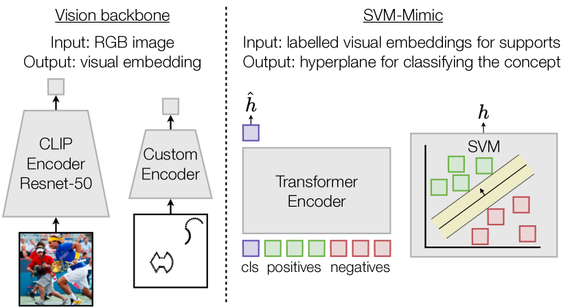
Crucially, we use an asymmetric student-teacher setup: the teacher (i.e., averaging or SVM) uses all available supports, yielding “clean” training targets. In fact, we allow the teachers to “cheat” by using labelled queries as additional supports. The student (i.e., the Transformer) receives only a random subset of supports, forcing it to learn to complete missing information. We refer to this step as “support dropout”. To make the learner’s task even more challenging, we use label noise: we randomly flip the positive/negative indicators for some supports (but leave the majority intact, to keep the problem well-posed). These training details encourage the Transformer to not only match the “simple baseline” teachers, but exceed them in terms of robustness to number of supports and errors in labels.

Another unique aspect of our approach is that we directly supervise the learning of (ideal) prototypes, or (max-margin) rules, with a regression loss. This is instead of supervising for the correct classification of queries, with for example a cross entropy loss. Our hypothesis is that this will focus the model on rule-making, which is a key aspect of Bongard problems in general.

When training a ResNet-12 backbone, we train both the backbone and the Transformer jointly by summing both loss terms. Note that it is possible to allow gradients to flow through the Transformer into the vision backbone, but for simplicity we omit this.

4 Experiments

To train our models, we used the AdamW optimizer (Loshchilov and Hutter 2017), a maximum learning rate of $5\mathrm{e}{-5}$, and a 1-cycle learning rate policy (Smith and Topin 2019), increasing the learning rate linearly for the first 5% of the training steps. We ran all experiments on NVIDIA Titan RTX, Titan XP, GeForce, or A5000 GPUs. All experiments used at most 1 GPU and 30GB of GPU memory. We selected hyperparameters by evaluating on the validation set for each dataset. Each experiment used at most 1 GPU and 30GB of GPU memory.

Method	Enc	Test (FF)	Test (BA)	Test (CM)	Test (NV)	Avg
SNAIL (Mishra et al. 2018)	RN12	56.3 $\pm$ 3.5	60.2 $\pm$ 3.6	60.1 $\pm$ 3.1	61.3 $\pm$ 0.8	59.5
ProtoNet (Snell, Swersky, and Zemel 2017)	RN12	64.8 $\pm$ 0.9	72.4 $\pm$ 0.8	62.4 $\pm$ 1.3	65.4 $\pm$ 1.2	66.3
MetaOptNet (Lee et al. 2019)	RN12	60.3 $\pm$ 0.6	71.7 $\pm$ 2.5	61.7 $\pm$ 1.1	63.3 $\pm$ 1.9	64.3
ANIL (Raghu et al. 2020)	RN12	56.6 $\pm$ 1.0	59.0 $\pm$ 2.0	59.6 $\pm$ 1.3	61.0 $\pm$ 1.5	59.1
Meta-Baseline-SC (Chen et al. 2020)	RN12	66.3 $\pm$ 0.6	73.3 $\pm$ 1.3	63.5 $\pm$ 0.3	63.9 $\pm$ 0.8	66.8
Meta-Baseline-MoCo (Nie et al. 2021)	RN12	65.9 $\pm$ 1.4	72.2 $\pm$ 0.8	63.9 $\pm$ 0.8	64.7 $\pm$ 0.3	66.7
WReN-Bongard (Barrett et al. 2018)	RN12	50.1 $\pm$ 0.1	50.9 $\pm$ 0.5	53.8 $\pm$ 1.0	54.3 $\pm$ 0.6	52.3
CNN-Baseline (Nie et al. 2021)	RN12	51.9 $\pm$ 0.5	56.6 $\pm$ 2.9	53.6 $\pm$ 2.0	57.6 $\pm$ 0.7	54.9
Meta-Baseline-PS (Nie et al. 2021)	RN12	68.2 $\pm$ 0.3	75.7 $\pm$ 1.5	67.4 $\pm$ 0.3	71.5 $\pm$ 0.5	70.7
TPT (Shu et al. 2022)	CLIP	52.5	65.9	58.6	56.3	58.3
PredRNet (Yang et al. 2023)	Other	74.6 $\pm$ 0.3	75.2 $\pm$ 0.6	71.1 $\pm$ 1.5	68.4 $\pm$ 0.7	72.3
Prototype	RN12	68.9 $\pm$ 0.5	68.8 $\pm$ 1.6	64.7 $\pm$ 0.8	66.2 $\pm$ 0.8	67.1 $\pm$ 0.7
Prototype + standardize	RN12	72.9 $\pm$ 0.5	80.8 $\pm$ 0.5	66.8 $\pm$ 1.1	71.3 $\pm$ 1.4	73.0 $\pm$ 0.8
SVM	RN12	65.7 $\pm$ 0.4	75.3 $\pm$ 1.3	65.4 $\pm$ 2.0	70.4 $\pm$ 1.6	69.2 $\pm$ 1.1
SVM + standardize	RN12	72.2 $\pm$ 0.3	83.8 $\pm$ 0.9	68.3 $\pm$ 1.6	71.8 $\pm$ 1.2	74.0 $\pm$ 0.5
$k$-NN	RN12	62.1 $\pm$ 0.7	69.3 $\pm$ 0.9	62.8 $\pm$ 0.6	63.3 $\pm$ 0.9	64.4 $\pm$ 0.4
$k$-NN + standardize	RN12	73.0 $\pm$ 0.6	84.9 $\pm$ 0.8	67.8 $\pm$ 1.8	71.0 $\pm$ 1.3	74.2 $\pm$ 0.5
Prototype-Mimic	RN12	73.1 $\pm$ 0.4	80.9 $\pm$ 0.6	68.4 $\pm$ 1.1	72.0 $\pm$ 0.9	73.6 $\pm$ 0.3
SVM-Mimic	RN12	73.3 $\pm$ 0.3	84.3 $\pm$ 0.8	69.4 $\pm$ 0.8	74.2 $\pm$ 0.3	75.3 $\pm$ 0.1
Human Expert (Nie et al. 2021)		92.1 $\pm$ 7.0	99.3 $\pm$ 1.9	90.7 $\pm$ 6.1		94.0
Human Amateur (Nie et al. 2021)		88.0 $\pm$ 7.6	90.0 $\pm$ 11.7	71.0 $\pm$ 9.6		83.0

Table 1: Results on Bongard-LOGO. Error bars are obtained by evaluating three trained models over the entire test set (thousands of problems), for all methods except deterministic ones.

Method	Unseen Act /	Seen Act /	Unseen Act /	Seen Act /	Avg
	Unseen Obj	Unseen Obj	Seen Obj	Seen Obj
HOITrans (Zou et al. 2021)	62.87	64.38	63.10	59.50	62.46
TPT (Shu et al. 2022)	65.66	65.32	68.70	66.03	66.43
Prototype	65.45	65.73	76.31	68.02	68.88
Prototype + standardize	68.11	68.92	77.44	69.97	71.11
SVM	68.05	67.36	74.89	67.91	69.55
SVM + standardize	69.48	69.50	75.37	69.68	71.01
$k$-NN	61.04	60.88	68.54	63.28	63.44
$k$-NN + standardize	66.72	67.08	75.65	68.04	69.37
Prototype-Mimic	68.88 $\pm$ 0.30	70.74 $\pm$ 0.44	76.66 $\pm$ 0.26	71.25 $\pm$ 0.29	71.88 $\pm$ 0.20
SVM-Mimic	69.59 $\pm$ 0.13	70.83 $\pm$ 0.27	78.13 $\pm$ 0.27	71.23 $\pm$ 0.07	72.45 $\pm$ 0.16
Human (Jiang et al. 2023)	87.21	90.01	93.61	94.85	91.42

Table 2: Results on Bongard-HOI with a frozen CLIP encoder. Error bars are obtained by evaluating three trained models over the entire test set (thousands of problems), for all methods except deterministic ones.

4.1 Bongard-LOGO

Dataset

We evaluate on the Bongard-LOGO dataset (Nie et al. 2021), which consists of synthetic images containing geometric shapes similar to those in the original Bongard problems. We follow previous works (Nie et al. 2021) and use a ResNet-12 (He et al. 2016) trained from scratch. Each Bongard-LOGO problem consists of seven positive and seven negative examples. The first six positives and first six negatives are chosen to serve as supports, and the remaining two are used as queries. We train models for 500,000 iterations with a batch size of 2. We resize images to $512\times 512$ pixels and apply random cropping and horizontal flipping to augment. We train all models using support dropout. Label noise did not improve results on the validation set (likely because the ground truth is error-free), so we omit it.

Results

Table 1 shows results on Bongard-LOGO’s four test splits, each assessing various forms of out-of-domain generalization. We observe that our simple baselines (Prototype, SVM, and $k$-NN) coupled with our contrastive encoder match or exceed most previous approaches. Incorporating standardization leads to a 5-10 point boost for each of them. The support-set Transformer models, Prototype-Mimic and SVM-Mimic, perform better than the non-Transformer variants. SVM-Mimic performs the best, with an accuracy of 75.3%. This is 3 points better than the the concurrent PredRNet (Yang et al. 2023). We note that while PredRNet performs well on Bongard-LOGO, it is not straightforward to extend it to natural image tasks like Bongard-HOI, since it cannot leverage arbitrary vision backbones, and relies on training end-to-end from scratch.

4.2 Bongard-HOI

Dataset

Bongard-HOI (Jiang et al. 2023) structures Bongard problems around natural images of human-object interaction. The positive support set of each problem involves a human interaction with an object, and the negative support set contains different interactions with the same object. Following a previous work (Shu et al. 2022), we use CLIP with a ResNet-50 backbone as our image encoder. The Bongard-HOI dataset is structured similarly to the Bongard-LOGO dataset, with seven positives and seven negatives per problem. Since the dataset does not specify the support/query split for each problem, we arbitrarily select the final positive and negative images as queries. We manually created a clean subset of the original training dataset after observing that the publicly-available Bongard-HOI dataset is imbalanced and contains incorrect labels (details in Appendix). We publicly release this cleaned training dataset to aid future works. We use augmentations at training time, including horizontal flips, random grayscale, color jitter, and random rescaling and cropping (to $224\times 224$), and apply support dropout and label noise. We train for 10,000 iterations with a batch size of 16 and weight decay of 0.01.

Results

Table 2 shows quantitative results on the four test splits of Bongard-HOI, each of which tests different forms of out-of-domain generalization. The “seen act/seen obj” split contains only human-object interactions where the actions and objects were both seen during training; “seen act/unseen obj” evaluates on problems with seen actions and unseen objects, and so on. We first note that our simple baselines (Prototype, SVM, and $k$-NN) approach or beat the state-of-the-art method, Test-time Prompt Tuning (TPT; Shu et al. (2022)). This is surprising, as none of these baselines uses training at any point, while TPT performs gradient descent at test time to find a classifier for each Bongard problem. We find that for every baseline, standardization leads to further performance improvements. For example, Prototype baseline combined with standardization exceeds TPT by almost 5 points. Using a support-set Transformer leads to further improvements. SVM-Mimic exceeds its counterpart baseline, SVM + standardize, by almost 1.5 points, setting a new state-of-the-art on Bongard-HOI.

4.3 Bongard-Classic

Dataset

Mikhail Bongard’s original dataset (Foundalis 2006; Yun, Bohn, and Ling 2020) is a challenging dataset of roughly 200 problems with no training or validation set. Since there is no training set, we directly evaluate backbones and support-set Transformers pre-trained on Bongard-LOGO. We perform the same data pre-processing steps as done for Bongard-LOGO. Since the dataset has six positive and six negative examples for each problem, we select one positive and one negative example as queries. For each Bongard problem, we average results over every possible choice of positive and negative query. Prior works use evaluation metrics other than accuracy, such as number of Bongard problems solved (Youssef et al. 2022) and accuracy on manually-created query images (Yun, Bohn, and Ling 2020). We use our own accuracy metric (percent correct total) as it is easier to calculate and is more consistent with Bongard-HOI and Bongard-LOGO.

Results

Table 3 shows the results of our approaches on Bongard-Classic. Due to the evaluation differences mentioned, we are unable to compare with other works, but we hope our results can serve as baselines for future work. Standardization leads to improvements in every case. Support-set Transformers do not lead to consistent improvements, likely because the Transformer has not been fine-tuned on Bongard-Classic problems. SVM-Mimic is our second-best performing method, attaining 60.84% accuracy.

Method	Accuracy
Prototype	57.52 $\pm$ 0.36
Prototype + standardize	57.82 $\pm$ 0.72
SVM	60.10 $\pm$ 0.55
SVM + standardize	61.27 $\pm$ 0.12
$k$-NN	56.80 $\pm$ 0.44
$k$-NN + standardize	58.10 $\pm$ 0.33
Prototype-Mimic	57.61 $\pm$ 0.89
SVM-Mimic	60.84 $\pm$ 0.43

Table 3: Results on Bongard-Classic. Error bars are obtained by evaluating three models over all 200 problems.

Method	Accuracy
PMF (Hu et al. 2022)	74.44 $\pm$ 0.22
Prototype + standardize + PMF	75.83 $\pm$ 0.20
SVM + standardize + PMF	75.42 $\pm$ 0.17
Prototype-Mimic + PMF	75.60 $\pm$ 0.14
SVM-Mimic + PMF	76.41 $\pm$ 0.14

Table 4: Results on Bongard-HOI with CLIP fine-tuned via PMF. For brevity, we average results over all test splits.

4.4 Cross-Image Context with Fine-Tuned CLIP

The state-of-the-art method for category-level few-shot learning tasks is PMF (Hu et al. 2022), and this technique involves fine-tuning the backbone encoder to produce better prototypes. This is complementary to our approach. Table 4 shows results from combining cross-image context with PMF, evaluated on Bongard-HOI. PMF has not previously been applied to Bongard problems, and it cannot be fairly compared with the methods in Table 2 due to the fine-tuned rather than frozen encoder. We combine support-set standardization, support-set Transformers, and our baselines with PMF by first fine-tuning the CLIP encoder with the PMF objective, freezing the weights, and then plugging the fine-tuned encoder directly into each method. PMF performs very well, exceeding the results obtained with frozen CLIP. Incorporating cross-image context through support-set standardization and support-set Transformers leads to further improvements. One failure case is Prototype-Mimic; note that the PMF training objective already optimizes the prototypes, so it is possible that the forward pass by the Transformer is not necessary. SVM-Mimic combined with PMF performs best. PMF training details are in the Appendix.

4.5 Robustness to Number of Supports

(a) Unseen Act, Unseen Obj

(b) Seen Act, Unseen Obj

(c) Unseen Act, Seen Obj

(d) Seen Act, Seen Obj

Figure 3: Robustness to number of supports in Bongard-HOI. The x-axis measures the number of supports of each class seen, with 6 being the default setting, and the y-axis measures accuracy. Means and standard deviations are reported across three runs, where the randomness is with respect to the subset of supports chosen.

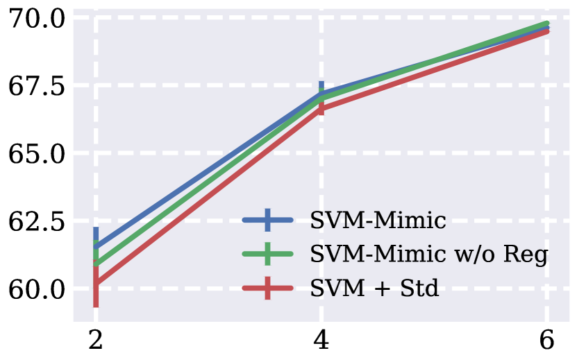
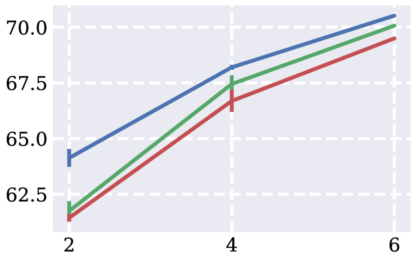
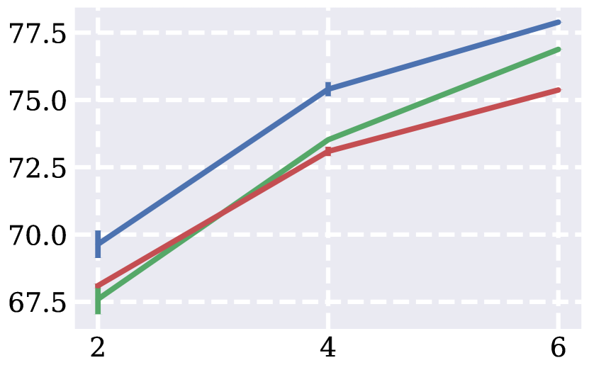
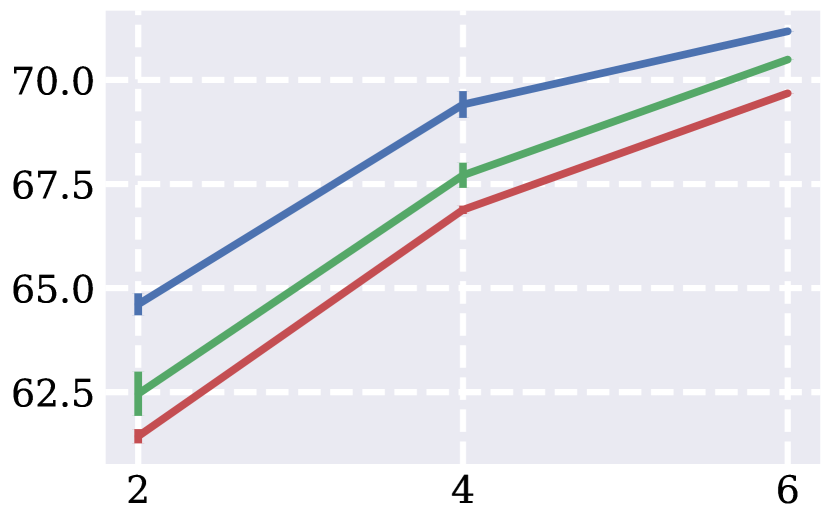
We are interested to measure SVM-Mimic’s robustness to the number of support samples provided as input. Figure 3 shows the results of SVM-Mimic, a version of SVM-Mimic trained without support dropout or label noise (SVM-Mimic w/o Reg), and SVM baseline + standardization (SVM + Std) on the test splits of Bongard-HOI. The plots demonstrate that SVM-Mimic attains consistently higher accuracy than the other approaches for different numbers of supports. This demonstrates the benefits of learning a Transformer to produce rules rather than non-parametrically fitting an SVM to each Bongard problem. In the Appendix, we also measure robustness to label noise.

4.6 Ablation Study: Forms of Normalization

Method	Accuracy
Prototype	68.88
Prototype + train-set standardize	70.06
Prototype + support-set standardize	71.11
SVM	69.55
SVM + $l^{2}$ normalization	67.94
SVM + train-set standardize	71.19
SVM + support-set standardize	71.01
$k$-NN	63.44
$k$-NN + train-set standardize	65.86
$k$-NN + support-set standardize	69.37

Table 5: Effect of different forms of normalization in Bongard-HOI. Results are averaged over the four test splits. Note that Prototype and $k$-NN use $l^{2}$ normalization by default.

Can support-set standardization be replaced with other forms of centering and scaling? Table 5 compares the performance of different forms of normalization on Bongard-HOI. “Support-set standardize” is our main approach; “train-set standardize” computes mean and variance statistics using the entire training set of CLIP embeddings; $l^{2}$ normalization normalizes each embedding independently. Importantly, neither train-set standardization nor $l^{2}$ normalization captures cross-image context at the task-level (instead focusing on the dataset-level and image-level). Train-set standardization leads to a 0.1 point gain over support-set standardization when using SVMs, but it performs 1 point worse with Prototypes and over 3 points worse with $k$-NN, suggesting that support-set standardization is a safe choice. We also find that $l^{2}$ normalization harms performance on the SVM, despite the fact that this is a design step included by default in Prototype and $k$-NN methods for computing cosine similarity.

5 Discussion and Conclusion

In this work, we point out that Bongard problems can only be solved by simultaneously considering positive and negative supports. We argue that it is necessary to acquire cross-image context from the entire support set. We demonstrate that support-set standardization, coupled with simple baselines, achieves state-of-the-art performance on Bongard-LOGO and Bongard-HOI. Second, we propose “mimicking” privileged teacher models with a student Transformer model and show that this leads to further improvements in accuracy. Our best model, SVM-Mimic, sets a new state-of-the-art on Bongard-LOGO and Bongard-HOI.

One limitation of our approach is sensitivity to the choice of encoder. It may be that as the strength of the encoder increases, the need for sophisticated cross-image context decreases, and statistical standardization may suffice. We also note that our Bongard-LOGO results appear to have benefited greatly from our contrastive learning stage, and perhaps other methods could be improved by incorporating our feature-learning technique.

Overall, our experiments attest to the importance of modeling cross-image context for Bongard problems. We hope that our results, our models, and our code will facilitate future work in this domain.

Acknowledgments. This work was supported by a Vannevar Bush Faculty Fellowship.

Appendix A Appendix

This appendix is intended to aid reproduction of our results and provide additional insight into performance of our methods. We first elaborate on model architectures and training details. Second, we give an overview of dataset licenses and cleaning procedures. Third, we demonstrate additional results. We finally provide extensive qualitative results.

Appendix B Experimental Details

Transformer Architecture

For both Bongard-LOGO and Bongard-HOI, we use a Transformer encoder with a depth of six, eight heads per layer, and 64 dimensions per head. We set the Transformer token and MLP dimensions to match the dimensionality of encoder outputs. For Bongard-HOI with a CLIP ResNet-50 backbone, this is 1024. For Bongard-LOGO with a ResNet-12 backbone, this is 128. For task outputs (prototypes and rules), we perform layer normalization on the Transformer’s output for the cls token(s) and transform them with a linear layer.

PMF Training Details

To train PMF, we use a maximum learning rate of $5\mathrm{e}{-7}$ and a batch size of 4 and train for 40,000 iterations. We use neither support dropout nor label noise. In order to train Prototype-Mimic using the PMF backbone, we observed that it was necessary to train for 40,000 iterations instead of the usual 10,000 iterations. We did not need to make any changes to the SVM-Mimic training procedure when using a PMF backbone.

Support Dropout Details

When using train-time support dropout, we always retain at least two supports from each class and at most all supports. We sample the same number of supports for each class.

Label Noise Details

When using train-time label noise, we only flip the labels of one positive and one negative support. We found it beneficial to apply label noise to only 25% of the training batches.

Appendix C Additional Dataset Details

Dataset Licenses

The datasets used in our experiments are all publicly available. The Bongard-LOGO dataset uses an MIT License. The Bongard-HOI dataset is open-sourced for research purposes. The dataset of problems from Mikhail Bongard (called Bongard-Classic in the paper) does not have a known license.

Method	Unseen Act /	Seen Act /	Unseen Act /	Seen Act /	Avg
(Both w/o Dropout)	Unseen Obj	Unseen Obj	Seen Obj	Seen Obj
SVM + standardize	69.48	69.50	75.37	69.68	71.01
SVM-Mimic, Full	69.88 $\pm$ 0.46	70.48 $\pm$ 0.20	77.24 $\pm$ 0.12	70.73 $\pm$ 0.32	72.08 $\pm$ 0.25
SVM-Mimic, Clean	69.59 $\pm$ 0.13	70.83 $\pm$ 0.27	78.13 $\pm$ 0.27	71.23 $\pm$ 0.07	72.45 $\pm$ 0.16

Table 6: Original Bongard-HOI training dataset vs. our cleaned dataset. Error bars are obtained by evaluating three trained models over the entire test set (thousands of problems).

Method	Unseen Act /	Seen Act /	Unseen Act /	Seen Act /	Avg
(Both w/o Dropout)	Unseen Obj	Unseen Obj	Seen Obj	Seen Obj
Prototype Set-to-Set-like	66.02 $\pm$ 0.93	71.22 $\pm$ 0.76	68.70 $\pm$ 0.71	70.69 $\pm$ 0.24	69.16 $\pm$ 0.23
Prototype-Mimic	68.88 $\pm$ 0.30	70.74 $\pm$ 0.44	76.66 $\pm$ 0.26	71.25 $\pm$ 0.29	71.88 $\pm$ 0.20

Table 7: Prototype-Mimic vs. Set-to-Set-like approach on Bongard-HOI. Error bars are obtained by evaluating three trained models over the entire test set (thousands of problems).

Cleaned Bongard-HOI Dataset

We observed that the Bongard-HOI dataset contains many incorrect labels and suffers from class imbalance. To mitigate this, we created a cleaned version of the train set and all validation sets. All SVM-Mimic results in our work were trained and validated on these cleaned sets but evaluated on the original Bongard-HOI test sets for fairest comparison with prior works. We manually curated these cleaned datasets. To do so, we first shuffled each Bongard problem’s positive and negative sets, and randomly selected one image in each set to serve as the positive and negative queries. For easy manual inspection, we cropped every image to the human-object-interaction of interest using annotations provided in the dataset, and resized the resulting image to a square. We then discarded all Bongard problems that did not meet all of the following criteria: (i) the object should be very clearly present in both query images, (ii) the positive query should demonstrate the interaction indicated in the label, and (iii) the negative query should not demonstrate the interaction. For faster curation, we did not inspect the support images. To ensure a balanced dataset, we sampled at most 100 Bongard problems for each unique human-object interaction in the train set, and 20 for each interaction in the validation sets. Our cleaned train set contained 2,196 problems, while the original train set contained 23,041 problems.

Table 6 contains results for SVM-Mimic models trained on the original and the cleaned train sets. These results demonstrate a very small but nearly consistent improvement from using the cleaned train set (despite the smaller size). The improvement justifies our use of the cleaned train set, but the small magnitude difference suggests that this cleaning is not critical. Both models outperform SVM + standardize.

Appendix D Additional Results

D.1 Robustness to Label Noise

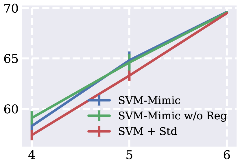
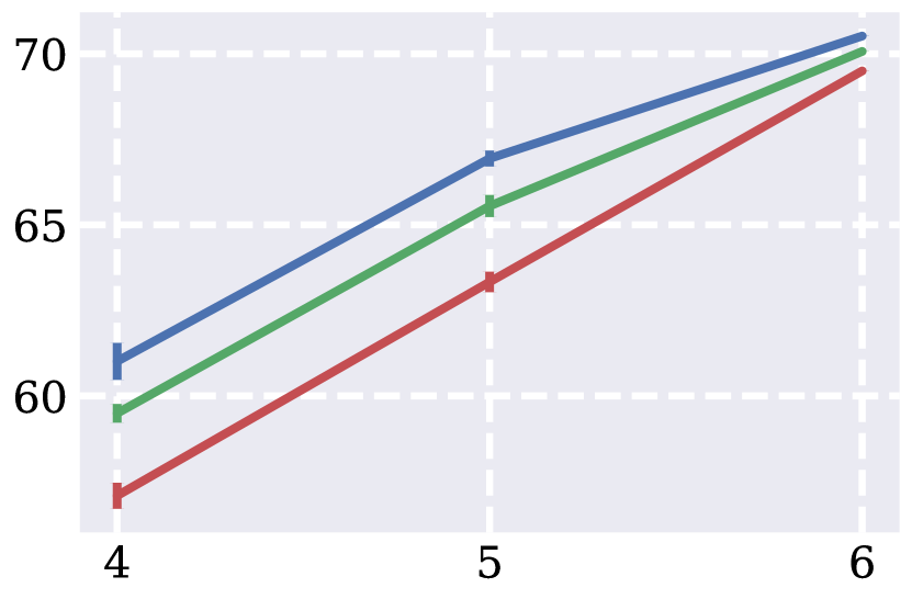
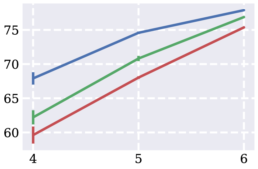
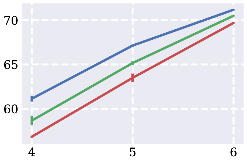
Figure 4 demonstrates the robustness of SVM-Mimic to noise in support labels, where noise is created by flipping the labels for random choices of positive and negative supports. In almost all cases, SVM-Mimic is clearly more robust than SVM-Mimic trained without support dropout or train-time label noise (SVM-Mimic w/o Reg) and SVM baseline + standardize (SVM + Std).

(a) Unseen Act, Unseen Obj

(b) Seen Act, Unseen Obj

(c) Unseen Act, Seen Obj

(d) Seen Act, Seen Obj

Figure 4: Robustness to label noise. The x-axis measures the number of supports of each class that have not been noised, with 6 being the default setting, and the y-axis measures accuracy. Means and standard deviations are reported across three runs, where the randomness is with respect to the subset of supports chosen.

D.2 Bongard-HOI Results with DINO Backbone

Table 8 contains results on Bongard-HOI using a DINO ViT-base backbone (Caron et al. 2021) instead of CLIP. Support-set standardization leads to consistent performance improvements for each of the three baselines. SVM-Mimic achieves a further performance boost of 0.54 points compared to SVM + standardize. One exception to the performance improvements is Prototype-Mimic, which fails to improve upon Prototype + standardize.

Implementation and training details

To obtain results using a DINO backbone, we use the same training procedure as for CLIP. We set the token and MLP dimensions at all layers of the Transformer to 768 to match DINO’s output dimensionality. We found it necessary to train SVM-Mimic for 20,000 iterations and Prototype-Mimic for 30,000 iterations.

Method	Unseen Act /	Seen Act /	Unseen Act /	Seen Act /	Avg
	Unseen Obj	Unseen Obj	Seen Obj	Seen Obj
Prototype	71.52	70.51	77.60	70.43	72.51
Prototype + standardize	72.33	72.81	79.19	71.19	73.88
SVM	72.77	71.77	78.35	70.29	73.29
SVM + standardize	73.14	72.06	78.24	70.71	73.54
$k$-NN	68.39	66.78	72.00	66.20	68.34
$k$-NN + standardize	70.47	71.05	76.62	68.90	71.76
Prototype-Mimic	71.57 $\pm$ 0.53	71.83 $\pm$ 0.25	76.74 $\pm$ 0.31	70.51 $\pm$ 0.25	72.66 $\pm$ 0.30
SVM-Mimic	73.07 $\pm$ 0.11	72.99 $\pm$ 0.22	78.97 $\pm$ 0.05	71.30 $\pm$ 0.15	74.08 $\pm$ 0.10

Table 8: Results on Bongard-HOI with a frozen DINO encoder.

D.3 Ablation Study: Comparison to Set-to-Set-like Approach

Rather than produce “rules” (hyperplanes or prototypes), it is possible for the Transformer to output support feature vectors that have been “adapted” using cross-image context. These adapted features can then be inputted into a downstream few-shot learning algorithm. This is similar to the “set-to-set” approach for few-shot learning (Ye et al. 2020). How does a set-to-set approach compare to our method? Table 7 compares Prototype-Mimic with a set-to-set-like approach that also produces prototypes on Bongard-HOI. Prototype-Mimic performs almost 2 points better, justifying our use of a rule-based method.

Implementation and training details

The set-to-set-like approach is trained identically to Prototype-Mimic, except the Transformer produces only “adapted” support feature vectors. These support feature vectors are converted into prototypes by averaging the vectors for each class, their cosine similarity to the queries are computed, and the model is trained with a cross-entropy loss. Due to overfitting, we train this set-to-set-like approach for only 2000 iterations. We use all normal Bongard-HOI training augmentations, including support dropout and label noise. We standardize all feature vectors using support set statistics before inputting support vectors into the Transformer.

Appendix E Qualitative Examples

In this section, we provide several qualitative examples on each dataset. Each example is a single Bongard problem with a positive and a negative query. We additionally report a score for each query using the margin between the query’s embedding and SVM-Mimic’s predicted hyperplane. Higher magnitude scores indicate greater distance between the query embedding and the hyperplane, which reflects greater confidence. To be classified correctly, positive queries should have a positive score and negative queries should have a negative score.

We compute these scores as $\frac{w\cdot f+b}{|w|}$, where $w$ and $b$ are the coefficients and intercept of the hyperplane and $f$ is the feature-space embedding of the query.

E.1 Bongard-HOI

We include examples on both the unseen action/unseen object test set as well as the unseen action/seen object test set.

E.2 Bongard-LOGO

The Bongard-LOGO test set consists of four splits. We refer to them using the abbreviations in the original Bongard-LOGO paper (Nie et al. 2021). In the free-form shape test set (FF) split, each support and query example consists of a free-form shape generated through Python “action programs”. None of these shapes was seen in training. Solving the problem requires determining which free-form shape is contained in all of the positive supports. In the basic shape (BA) test set, the concept binding all positive examples together is the composition of two basic shapes. Each of these compositions was not seen in training. In the combinatorial abstract shape (CM) test set, the concepts are abstract attributes of shapes (e.g., “has four straight lines”). Each problem contains the composition of two of these concepts. While each individual concept has been seen in training, the combination of the concepts is novel. The novel abstract shape (NV) test set is similar, except one of the concepts was never seen in training.

E.3 Bongard-Classic

We additionally include a few examples on the challenging Bongard-Classic dataset.

(a) Positive supports.

(b) Negative supports.

(c) Pos Que. Score: 9.0.

(d) Neg Que. Score: -4.2.

Figure 5: Bongard-HOI unseen act/seen obj: Correct guess for both queries. The concept is “turn motorcycle.”

(a) Positive supports.

(b) Negative supports.

(c) Pos Que. Score: 0.4.

(d) Neg Que. Score: -2.1.

Figure 6: Bongard-HOI unseen act/seen obj: Correct guess for both queries. The concept is “read laptop.”

(a) Positive supports.

(b) Negative supports.

(c) Pos Que. Score: 3.0.

(d) Neg Que. Score: 5.6.

Figure 7: Bongard-HOI unseen act/seen obj: Correct for positive, incorrect for negative. The concept is “grind skateboard.”

(a) Positive supports.

(b) Negative supports.

(c) Pos Que. Score: -8.7.

(d) Neg Que. Score: -7.1.

Figure 8: Bongard-HOI unseen act/seen obj: Incorrect for positive, correct for negative. The concept is “turn motorcycle.”

References

- Barrett et al. (2018) Barrett, D.; Hill, F.; Santoro, A.; Morcos, A.; and Lillicrap, T. 2018. Measuring abstract reasoning in neural networks. In International conference on machine learning, 511–520. PMLR.
- Bongard (1968) Bongard, M. M. 1968. The recognition problem. Foreign Technology Div Wright-Patterson AFB Ohio.
- Caron et al. (2021) Caron, M.; Touvron, H.; Misra, I.; Jégou, H.; Mairal, J.; Bojanowski, P.; and Joulin, A. 2021. Emerging properties in self-supervised vision transformers. In Proceedings of the IEEE/CVF international conference on computer vision, 9650–9660.
- Chen et al. (2021) Chen, Y.; Liu, Z.; Xu, H.; Darrell, T.; and Wang, X. 2021. Meta-baseline: Exploring simple meta-learning for few-shot learning. In Proceedings of the IEEE/CVF International Conference on Computer Vision, 9062–9071.
- Chen et al. (2020) Chen, Y.; Wang, X.; Liu, Z.; Xu, H.; Darrell, T.; et al. 2020. A new meta-baseline for few-shot learning. arXiv preprint arXiv:2003.04390, 2(3): 5.
- Depeweg, Rothkopf, and Jäkel (2018) Depeweg, S.; Rothkopf, C. A.; and Jäkel, F. 2018. Solving bongard problems with a visual language and pragmatic reasoning. arXiv preprint arXiv:1804.04452.
- Fei-Fei, Fergus, and Perona (2006) Fei-Fei, L.; Fergus, R.; and Perona, P. 2006. One-shot learning of object categories. IEEE transactions on pattern analysis and machine intelligence, 28(4): 594–611.
- Finn, Abbeel, and Levine (2017) Finn, C.; Abbeel, P.; and Levine, S. 2017. Model-agnostic meta-learning for fast adaptation of deep networks. In International conference on machine learning, 1126–1135. PMLR.
- Foundalis (2006) Foundalis, H. E. 2006. Phaeaco: A Cognitive Architecture Inspired by Bongard’s Problems. Ph.D. thesis, Indiana University Southeast.
- Greff, van Steenkiste, and Schmidhuber (2020) Greff, K.; van Steenkiste, S.; and Schmidhuber, J. 2020. On the Binding Problem in Artificial Neural Networks. arXiv:2012.05208.
- Grinberg et al. (2023) Grinberg, T.; Grinberg, D.; Shcherbanskiy, G.; and Cherbanski, L. 2023. Bongard Architecture: Towards Scalable and Transparent Machine Reasoning. In AAAI Spring Symposium Series 2023: Evaluation and Design of Generalist Systems.
- He et al. (2020) He, K.; Fan, H.; Wu, Y.; Xie, S.; and Girshick, R. 2020. Momentum contrast for unsupervised visual representation learning. In Proceedings of the IEEE/CVF conference on computer vision and pattern recognition, 9729–9738.
- He et al. (2016) He, K.; Zhang, X.; Ren, S.; and Sun, J. 2016. Deep residual learning for image recognition. In Proceedings of the IEEE conference on computer vision and pattern recognition, 770–778.
- Hearst et al. (1998) Hearst, M. A.; Dumais, S. T.; Osuna, E.; Platt, J.; and Scholkopf, B. 1998. Support vector machines. IEEE Intelligent Systems and their applications, 13(4): 18–28.
- Hofstadter (1979) Hofstadter, D. R. 1979. Godel, Escher, Bach: An Eternal Golden Braid. Basic Books, Inc., New York.
- Hu et al. (2022) Hu, S. X.; Li, D.; Stühmer, J.; Kim, M.; and Hospedales, T. M. 2022. Pushing the limits of simple pipelines for few-shot learning: External data and fine-tuning make a difference. In CVPR, 9068–9077.
- Jain, Duin, and Mao (2000) Jain, A. K.; Duin, R. P. W.; and Mao, J. 2000. Statistical pattern recognition: A review. IEEE Transactions on pattern analysis and machine intelligence, 22(1): 4–37.
- Jiang et al. (2023) Jiang, H.; Ma, X.; Nie, W.; Yu, Z.; Zhu, Y.; Zhu, S.-C.; and Anandkumar, A. 2023. Bongard-HOI: Benchmarking Few-Shot Visual Reasoning for Human-Object Interactions. arXiv:2205.13803.
- Lake, Salakhutdinov, and Tenenbaum (2015) Lake, B. M.; Salakhutdinov, R.; and Tenenbaum, J. B. 2015. Human-level concept learning through probabilistic program induction. Science, 350(6266): 1332–1338.
- Lee et al. (2019) Lee, K.; Maji, S.; Ravichandran, A.; and Soatto, S. 2019. Meta-learning with differentiable convex optimization. In Proceedings of the IEEE/CVF conference on computer vision and pattern recognition, 10657–10665.
- Linhares (2000) Linhares, A. 2000. A glimpse at the metaphysics of Bongard problems. Artificial Intelligence, 121(1-2): 251–270.
- Loshchilov and Hutter (2017) Loshchilov, I.; and Hutter, F. 2017. Decoupled weight decay regularization. arXiv preprint arXiv:1711.05101.
- Maksimov and Bongard (1968) Maksimov, V.; and Bongard, M. 1968. A Program that Learns to Classify Geometrical Figures. IFAC Proceedings Volumes, 2(4): 771–775.
- Mensink et al. (2013) Mensink, T.; Verbeek, J.; Perronnin, F.; and Csurka, G. 2013. Distance-based image classification: Generalizing to new classes at near-zero cost. IEEE transactions on pattern analysis and machine intelligence, 35(11): 2624–2637.
- Miller, Matsakis, and Viola (2000) Miller, E. G.; Matsakis, N. E.; and Viola, P. A. 2000. Learning from one example through shared densities on transforms. In Proceedings IEEE Conference on Computer Vision and Pattern Recognition. CVPR 2000 (Cat. No. PR00662), volume 1, 464–471. IEEE.
- Mishra et al. (2018) Mishra, N.; Rohaninejad, M.; Chen, X.; and Abbeel, P. 2018. A Simple Neural Attentive Meta-Learner. arXiv:1707.03141.
- Mitchell (2021) Mitchell, M. 2021. Abstraction and analogy-making in artificial intelligence. Annals of the New York Academy of Sciences, 1505(1): 79–101.
- Nie et al. (2021) Nie, W.; Yu, Z.; Mao, L.; Patel, A. B.; Zhu, Y.; and Anandkumar, A. 2021. Bongard-LOGO: A New Benchmark for Human-Level Concept Learning and Reasoning. arXiv:2010.00763.
- Radford et al. (2021) Radford, A.; Kim, J. W.; Hallacy, C.; Ramesh, A.; Goh, G.; Agarwal, S.; Sastry, G.; Askell, A.; Mishkin, P.; Clark, J.; et al. 2021. Learning transferable visual models from natural language supervision. In International conference on machine learning, 8748–8763. PMLR.
- Raghu et al. (2020) Raghu, A.; Raghu, M.; Bengio, S.; and Vinyals, O. 2020. Rapid Learning or Feature Reuse? Towards Understanding the Effectiveness of MAML. arXiv:1909.09157.
- Raven (1956) Raven, J. 1956. Guide to progressive matrices (Rev. ed.). London, UK: HK Lewis.(Original work published 1938).
- Shu et al. (2022) Shu, M.; Nie, W.; Huang, D.-A.; Yu, Z.; Goldstein, T.; Anandkumar, A.; and Xiao, C. 2022. Test-Time Prompt Tuning for Zero-Shot Generalization in Vision-Language Models.
- Smith and Topin (2019) Smith, L. N.; and Topin, N. 2019. Super-convergence: Very fast training of neural networks using large learning rates. In Artificial intelligence and machine learning for multi-domain operations applications, volume 11006, 369–386. SPIE.
- Snell, Swersky, and Zemel (2017) Snell, J.; Swersky, K.; and Zemel, R. 2017. Prototypical networks for few-shot learning. Advances in Neural Information Processing Systems, 30.
- Sonwane et al. (2021) Sonwane, A.; Chitlangia, S.; Dash, T.; Vig, L.; Shroff, G.; and Srinivasan, A. 2021. Using Program Synthesis and Inductive Logic Programming to solve Bongard Problems. arXiv:2110.09947.
- Spratley, Ehinger, and Miller (2020) Spratley, S.; Ehinger, K.; and Miller, T. 2020. A closer look at generalisation in raven. In Computer Vision–ECCV 2020: 16th European Conference, Glasgow, UK, August 23–28, 2020, Proceedings, Part XXVII 16, 601–616. Springer.
- Thrun and Pratt (2012) Thrun, S.; and Pratt, L. 2012. Learning to learn. Springer Science & Business Media.
- Vaswani et al. (2017) Vaswani, A.; Shazeer, N.; Parmar, N.; Uszkoreit, J.; Jones, L.; Gomez, A. N.; Kaiser, Ł.; and Polosukhin, I. 2017. Attention is all you need. Advances in Neural Information Processing Systems, 30.
- Vinyals et al. (2016) Vinyals, O.; Blundell, C.; Lillicrap, T.; Wierstra, D.; et al. 2016. Matching networks for one shot learning. Advances in neural information processing systems, 29.
- Yang et al. (2023) Yang, L.; You, H.; Zhen, Z.; Wang, D.; Wan, X.; Xie, X.; and Zhang, R.-Y. 2023. Neural Prediction Errors enable Analogical Visual Reasoning in Human Standard Intelligence Tests. In ICML.
- Ye et al. (2020) Ye, H.-J.; Hu, H.; Zhan, D.-C.; and Sha, F. 2020. Few-shot learning via embedding adaptation with set-to-set functions. In Proceedings of the IEEE/CVF conference on computer vision and pattern recognition, 8808–8817.
- Youssef et al. (2022) Youssef, S.; Zečević, M.; Dhami, D. S.; and Kersting, K. 2022. Towards a Solution to Bongard Problems: A Causal Approach. arXiv:2206.07196.
- Yun, Bohn, and Ling (2020) Yun, X.; Bohn, T.; and Ling, C. 2020. A deeper look at Bongard problems. In Advances in Artificial Intelligence: 33rd Canadian Conference on Artificial Intelligence, Canadian AI 2020, Ottawa, ON, Canada, May 13–15, 2020, Proceedings 33, 528–539. Springer.
- Zhang et al. (2019) Zhang, C.; Gao, F.; Jia, B.; Zhu, Y.; and Zhu, S.-C. 2019. Raven: A dataset for relational and analogical visual reasoning. In Proceedings of the IEEE/CVF conference on computer vision and pattern recognition, 5317–5327.
- Zhou et al. (2022) Zhou, K.; Yang, J.; Loy, C. C.; and Liu, Z. 2022. Learning to prompt for vision-language models. International Journal of Computer Vision, 130(9): 2337–2348.
- Zou et al. (2021) Zou, C.; Wang, B.; Hu, Y.; Liu, J.; Wu, Q.; Zhao, Y.; Li, B.; Zhang, C.; Zhang, C.; Wei, Y.; and Sun, J. 2021. End-to-End Human Object Interaction Detection with HOI Transformer. arXiv:2103.04503.