Distribution-Aware Prompt Tuning for Vision-Language Models

Abstract

Pre-trained vision-language models (VLMs) have shown impressive performance on various downstream tasks by utilizing knowledge learned from large data. In general, the performance of VLMs on target tasks can be further improved by prompt tuning, which adds context to the input image or text. By leveraging data from target tasks, various prompt-tuning methods have been studied in the literature. A key to prompt tuning is the feature space alignment between two modalities via learnable vectors with model parameters fixed. We observed that the alignment becomes more effective when embeddings of each modality are ‘well-arranged’ in the latent space. Inspired by this observation, we proposed distribution-aware prompt tuning (DAPT) for vision-language models, which is simple yet effective. Specifically, the prompts are learned by maximizing inter-dispersion, the distance between classes, as well as minimizing the intra-dispersion measured by the distance between embeddings from the same class. Our extensive experiments on 11 benchmark datasets demonstrate that our method significantly improves generalizability. The code is available at https://github.com/mlvlab/DAPT.

1 Introduction

Text
Image

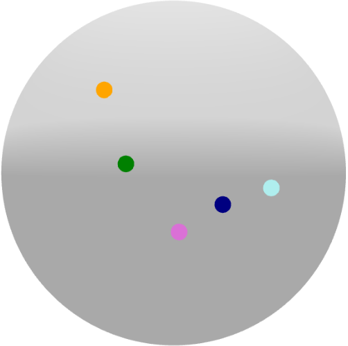
(a)

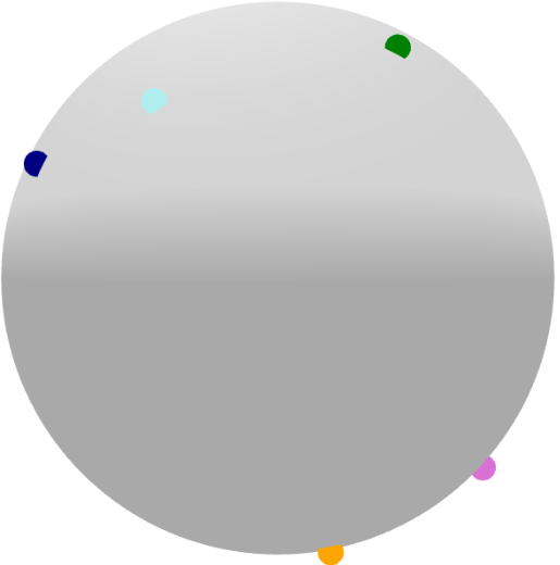
(b)

(c)

(d)

Figure 1: Points in (a) and (b) denote normalized t-SNE embeddings of text features from OxfordPets [26]. In addition, points on (c) and (d) represent the image features’ t-SNE embeddings from EuroSAT [12]. As shown in (a) and (b), zero-shot CLIP has small distances between text embeddings of class labels, but its image embeddings do not cluster well. However, prompt-tuning with DAPT leads to more evenly spaced text embeddings and better clusterings of image embeddings within the same class.

In recent years, pre-trained vision-language models (VLMs) have shown great success in a wide range of applications in computer vision such as image classification [29, 33], object detection [7, 11, 44], captioning [21, 24, 42], and visual question answering (VQA) [9]. Notably, VLMs have shown promising generalization power and transferability in various downstream tasks. For instance, VLMs such as CLIP [29] and ALIGN [15] show outstanding performance in zero-shot and few-shot learning. These models opened the door for zero-shot image classification and zero-shot object detection. To further improve the pre-trained models’ zero-shot generalization ability, prompting has been proposed. For instance, in image classification, CLIP [29] suggests using a context text “A photo of a ” in front of the class label [CLASS] to obtain text embeddings for target classes.

Prompting is an emerging research topic due to several advantages over fine-tuning, which is a conventional approach to utilize pre-trained deep-learning models. For a pre-trained VLM, fine-tuning is often practically challenging due to the large number of model parameters. In addition, fine-tuning the entire VLM often results in overfitting due to a small amount of target domain data. Zhou et al. [47] have shown that more powerful context strings (hard prompts) exist. However, manually finding better hard prompts (prompt engineering) is time-consuming and suboptimal. So, after that, a line of works has proposed prompt-tuning that optimizes soft prompts, learnable vectors [16, 20, 47]. The learnable vectors are concatenated with other inputs and numerically optimized by backpropagation while the pre-trained VLM models parameters are fixed.

The prompt tuning can be viewed as the alignment between two latent spaces of text and image. Figure 1 shows that each latent space of CLIP is not suitable for feature alignment. The text embeddings of target classes obtained from the original CLIP in Figure 1(a) are gathered nearby, which potentially leads to misclassification to close classes. In addition, the original CLIP’s visual embeddings in Figure 1(c) are widely spread, and some regions are overlapped. To address this problem, we propose a prompt tuning method, DAPT, that optimizes the distribution of embeddings for each modality for better feature alignment.

DAPT learns vectors (i.e., soft prompts) for both text and image encoders with additional loss terms - inter-dispersion loss and intra-dispersion loss. Specifically, we apply the inter-dispersion loss to the text prompts to spread text embeddings. On the other hand, intra-dispersion loss is applied to the visual prompts to minimize the variability of image embeddings of the same class.

To verify the effectiveness of DAPT, we conducted experiments on few-shot learning and domain generalization tasks with various benchmark datasets. For few-shot learning with one sample (1-shot) to 16 samples (16-shots) per class, the proposed method is evaluated on 11 benchmark datasets. For domain generalization, 4 benchmark datasets were used after few-shot learning on ImageNet [5]. Overall, we achieve a significant improvement over recent baselines for few-shot learning and domain generalization.

In summary, we propose DAPT, a prompt tuning method that is aware of the data distributions to improve the performance of VLMs in the few-shot learning setup. Unlike the orthodox prompt tuning method, DAPT optimizes text and visual prompts to find the appropriate distribution in each modality. In Section 3, we discuss the details of DAPT and show the various experiments in Section 4.

2 Related Work

Pre-Trained Vision-Language Models. Pre-trained vision-language models (VLMs) [15, 29, 40, 43] jointly learn text and image embeddings with large-scale noisy image-text paired datasets. Out of those, CLIP [29] and ALIGN [15] optimize cross-modal representations between positive pairs via contrastive learning and demonstrate impressive performance in various downstream tasks [7, 11, 21, 24, 42, 45]. In addition, there are approaches to enhance the ability of VLMs by adjusting latent space in succeeding research. For instance, Wang et al. [38] claim that alignment and uniformity are two key properties to optimize. By expanding these properties, Goel et al. [10] propose CyCLIP to mitigate inconsistent prediction in CLIP, fixing the CLIP embedding geometry.

Prompt Tuning. Prompting has been studied in natural language processing (NLP). Prompt tuning methods such as Petroni et al. [28], Shin et al. [32], and Jiang et al. [17] are proposed to construct suitable prompt template. Under the influence of NLP, prompt tuning methods with vision-language models are actively studied in the computer vision domain. Unlike the hard prompts suggested in CLIP [29], several works have studied soft prompts by optimizing learnable vectors in text or visual modality. CoOp [47] composes prompt concatenated with label embedding and learnable vectors by the text encoder. CoCoOp [46] is an advanced version of CoOp and improves generalizability in unseen classes. Also, VPT [16] and VP [1] propose prompt tuning on the visual modality. VPT uses learnable vectors for prompt tuning in the Vision Transformer [6]. Different from prior works, VP suggests image pixel-level prompt tuning in CLIP image encoder. Those prompt tuning methods show remarkable transferability and generalizability with only a few parameters. More recently, ProDA [22] and PLOT [3] use multiple prompts and demonstrate better performance than a single text prompt. Based on recent success in prompt tuning, there are multimodal prompt tuning methods in VLMs. UPT [41] jointly optimize modality-agnostic prompts with extra layers. MVLPT [31] focuses on multi-task prompting. MaPLe [18] improves generalizability of VLMs via multimodal prompting.

3 Method

In this section, we briefly revisit the CLIP [29] and the several prompt tuning methods [16, 47] in Section 3.1. Then we propose a distribution-aware prompt tuning, DAPT, in Section 3.2 in detail.

3.1 Preliminaries

CLIP [29] is a vision-language model which trained via contrastive learning on a massive number of image-text pairs. In general, CLIP consists of image encoder $f$ and text encoder $g$. Given an image $\boldsymbol{x}$ and text label $\boldsymbol{t}$, image embedding $\boldsymbol{z}$ and text embedding $\boldsymbol{w}$ can be obtained as follows:

$$\boldsymbol{z}=f(\boldsymbol{x})$$ (1)

$$\boldsymbol{w}=g(\boldsymbol{t}).$$ (2)

Note that image embedding $\boldsymbol{z}$ and text embedding $\boldsymbol{w}$ are normalized. Given $C$ image classes, the prediction probability can be calculated by softmax with the cosine similarity between the image embeddings and the corresponding text embeddings representing the image class given as:

$$\begin{split}&p(y=c|\boldsymbol{x})=\cfrac{\exp{(\boldsymbol{z}^{\top}\boldsymbol{w}_{c}/\tau})}{{\sum_{j=1}^{C}}\exp{(\boldsymbol{z}^{\top}\boldsymbol{w}_{j}/\tau})},\end{split}$$ (3)

where $\tau$ is a temperature parameter, and $\boldsymbol{w}_{c}$ represents the text embedding of the class label $\boldsymbol{t}_{c}$. Combining with cross-entropy, we define CLIP loss, $\mathcal{L}_{\text{CLIP}}$, as follows:

$$\begin{split}&\mathcal{L}_{\text{CLIP}}=-\frac{1}{B}\sum_{i=1}^{B}\log\frac{\exp{(\boldsymbol{z}_{i}^{\top}\boldsymbol{w}_{y_{i}}/\tau)}}{\sum_{j=1}^{C}{\exp{(\boldsymbol{z}_{i}^{\top}\boldsymbol{w}_{j}/\tau}})},\end{split}$$ (4)

where $y_{i}$ denotes the class of $i$-th image $\boldsymbol{x}$, and $B$ is the batch of image-text pairs.

Text Prompt. CoOp [47] is the first approach to apply prompt tuning in the text encoder of CLIP. In CoOp, text prompt $\boldsymbol{p}$ is represented as a learnable vector $v$ combined with the class. Then, the input of the text encoder is given as:

$$\boldsymbol{p}_{j}=[v_{1},v_{2},\cdots,v_{L},\texttt{CLASS}].$$ (5)

The output of the text encoder with soft prompts is represented as:

$$\tilde{\boldsymbol{w}}_{j}=g(\boldsymbol{p}_{j}).$$ (6)

Note that ${\tilde{\boldsymbol{w}}}$ is normalized. CoOp uses various configurations with respect to the length $L$ and positions depending on datasets. They can be viewed as hyperparameters for prompt tuning. In our method, we fixed the hyperparameters for all settings. The learnable vectors of the text prompt are placed in front of CLASS with a length of $L=16$.

Visual Prompt. In the computer vision domain, VPT [16] proposed a visual prompt tuning method for Vision Transformers (ViT) [6]. Similar to CoOp, VPT inserts the learnable vector $u$ between class token $\mathtt{CLS}$ and image patch embeddings $\boldsymbol{E}$ for the image encoder. Since CLIP [29] uses ViT backbone for the image encoder, we define the visual prompt in CLIP as below:

$$\begin{split}&\boldsymbol{q}_{i}=[\mathtt{CLS},u_{1},u_{2}\cdots,u_{L},\boldsymbol{E}].\end{split}$$ (7)

We set the length of learnable vectors of the visual prompt to $L=16$, which is the same as the text prompt in (5). From (LABEL:eq:visual_prompt), we can obtain output image embedding $\tilde{\boldsymbol{z}}_{i}$ with visual prompt $\boldsymbol{q}_{i}$ as:

$$\begin{split}&\tilde{\boldsymbol{z}}_{i}=f(\boldsymbol{q}_{i}).\end{split}$$ (8)

Note that ${\tilde{\boldsymbol{z}}}$ is normalized.

Prompt Tuning. When fine-tuning CLIP with prompts, the image encoder and the text encoder have typically frozen the weights of all layers. Therefore, only the prompts are optimized. For large-scale pre-trained models, prompt tuning is often more effective and efficient than traditional fine-tuning methods such as linear probing and full fine-tuning of all layers.

3.2 Distribution-Aware Prompt Tuning

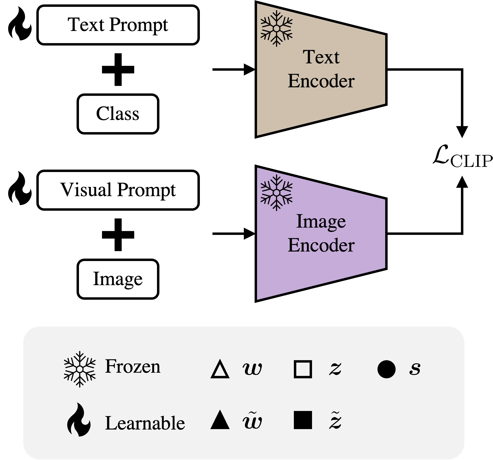
(a)

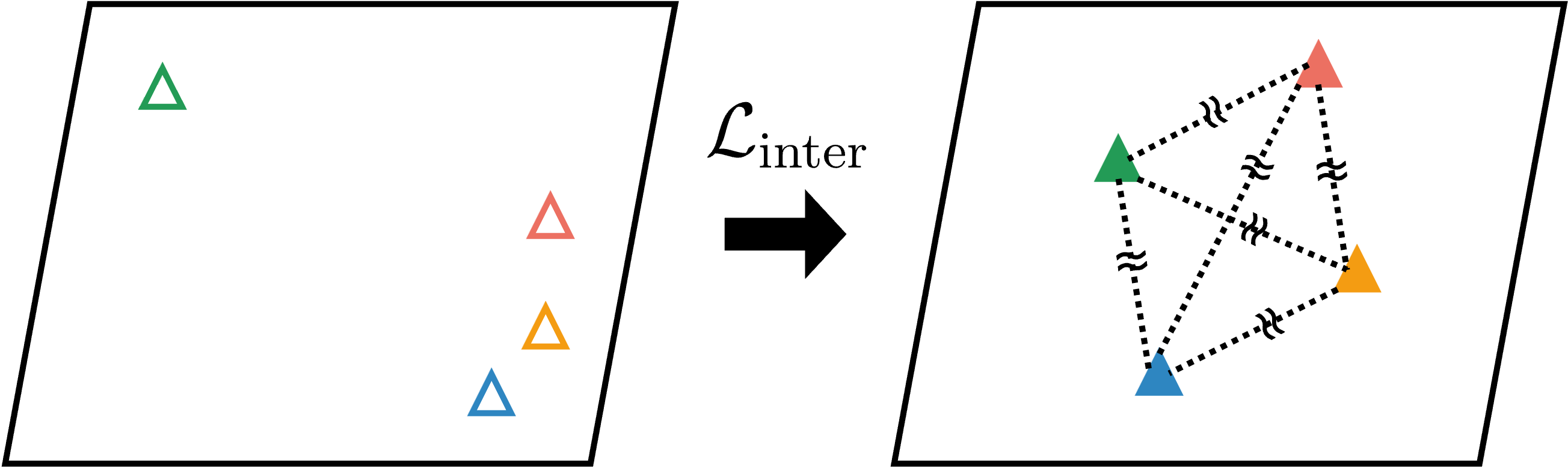
(b)

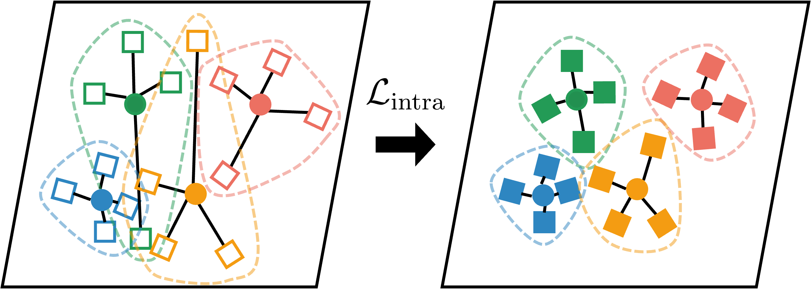
(c)

Figure 2: Overall architecture of DAPT. (a) DAPT consists of CLIP [29] architecture combined with CoOp [47] and VPT [16]. The symbols mean text and visual output embedding (i.e., $\boldsymbol{w}$ and $\boldsymbol{z}$), text and visual outputs combined with prompts (i.e., $\tilde{\boldsymbol{w}}$ and $\tilde{\boldsymbol{z}}$), and the prototype $\boldsymbol{s}$. Following prompt tuning manner, text and image encoders are frozen during training, and only prompts are updated. (b) Inter-dispersion loss $\mathcal{L}_{\text{inter}}$ defined from Gaussian potential kernel $\mathrm{G}$ is applied to text prompts to expand the distance between each text embeddings $\tilde{\boldsymbol{w}}$ to avoid embedding collapse. (c) To aggregate image embeddings within the same class, we define the prototype $\boldsymbol{s}$ demonstrates representative image embeddings of each class by calculating the average of zero-shot CLIP image embeddings $\boldsymbol{z}$. Then, intra-dispersion loss $\mathcal{L}_{\text{intra}}$ is applied to the visual prompt to gather image embeddings around the prototype $\boldsymbol{s}$.

We present DAPT that improves feature alignment between text and visual modalities by optimizing the distributions of embeddings via inter-dispersion and intra-dispersion losses. The overall pipeline of the proposed method is presented in Figure 2 and how inter-dispersion and intra-dispersion losses optimize text and visual latent spaces is depicted in Figure 2(b) and 2(c), respectively.

Inter-Dispersion Loss for Text Prompts. A small distance between text (label) embeddings may lead to misclassification and make it difficult to align visual features. To address this issue, we introduce an inter-dispersion loss in text embeddings based on the uniformity inspired by Wang et al. [38]. Uniformity means that the feature embeddings are roughly uniformly distributed in the hypersphere. This minimizes the overlap between embeddings and enables better alignment. With normalized text embeddings $\tilde{\boldsymbol{w}}$, we define Gaussian potential kernel $\mathrm{G}$ as follows:

$$\begin{split}&\mathrm{G}(\tilde{\boldsymbol{w}}_{m},\tilde{\boldsymbol{w}}_{n}):=\exp{(-t\|\tilde{\boldsymbol{w}}_{m}-\tilde{\boldsymbol{w}}_{n}\|^{2}_{2})},\end{split}$$ (9)

where $m,n\in C$ and $m\neq n$.

Minimizing the Gaussian potential kernel $\mathrm{G}$ above increases the distance between the text embeddings of prompt $\boldsymbol{p}_{m}$ and $\boldsymbol{p}_{n}$ on the hypersphere. To optimize the distribution of text embeddings encouraging uniformity, we define the inter-dispersion loss as follows:

$$\mathcal{L}_{\text{inter}} =\sum_{m\neq n}\mathrm{G}(\tilde{\boldsymbol{w}}_{m},\tilde{\boldsymbol{w}}_{n})$$ (10)

$$=\sum_{m\neq n}\exp{(-t{\|\tilde{\boldsymbol{w}}_{m}-\tilde{\boldsymbol{w}}_{n}\|}_{2}^{2})}.$$ (11)

Note that we set hyperparameter $t=2$ for all experiments in this paper.

Intra-Dispersion Loss for Visual Prompts. Given a class, unlike the uniquely defined text (label) embedding, multiple visual embeddings exist in the latent space. Specifically, due to multiple images per class in the dataset, various image embeddings are obtained from the image encoder.

For better alignment between the text and image embeddings given class $\boldsymbol{t}_{c}$, image embeddings of the same class should be close to each other. To reduce the intra-class distance of image embeddings $\tilde{\boldsymbol{z}}_{i}$ and $\tilde{\boldsymbol{z}}_{j}$, we define the prototype $\boldsymbol{s}$ motivated by PROTONET [34] with training samples $\mathcal{D}_{N}=\{(\boldsymbol{x}_{i},\boldsymbol{y}_{i})\}_{i=1}^{N}$ as follows:

$$\begin{split}&\boldsymbol{s}_{c}=\cfrac{1}{N}\sum_{(\boldsymbol{x}_{i},\boldsymbol{y}_{i})\in\mathcal{D}_{N}^{c}}{\boldsymbol{z}_{i}},\end{split}$$ (12)

where $\boldsymbol{z}_{i}=f(\boldsymbol{x}_{i})$. Note that $\mathcal{D}^{c}_{N}=\{(\boldsymbol{x}_{i},\boldsymbol{y}_{i})\in\mathcal{D}_{N}|\boldsymbol{y}_{i}=c\}$ and $N$ is the number of training samples. In order to cluster image embeddings with the same class, we assume that each embedding should be close to its prototype. Therefore, the intra-dispersion loss $\mathcal{L}_{\text{intra}}$, which reduces the distance between the image embedding and the prototype $\boldsymbol{s}$, is defined as follows:

$$\begin{split}&\mathcal{L}_{\text{intra}}=\sum_{c}\sum_{i}\mathbbm{1}_{[y_{i}=c]}{\|\tilde{\boldsymbol{z}}_{i}-\boldsymbol{s}_{c}\|}_{2}^{2},\end{split}$$ (13)

where $c$ is the corresponding class index of input image $\boldsymbol{x}_{i}$.

Optimization. Combining the CLIP loss in (4), our dispersion losses in (11) and (LABEL:eq:intra_loss), DAPT optimizes text prompt $\boldsymbol{p}$ from  (5) and visual prompt $\boldsymbol{q}$ from  (LABEL:eq:visual_prompt) by minimizing the following total loss:

$$\begin{split}&\mathcal{L}=\mathcal{L}_{\text{CLIP}}+\beta_{t}\mathcal{L}_{\text{inter}}+\beta_{v}\mathcal{L}_{\text{intra}},\end{split}$$ (14)

where $\beta_{t}$ and $\beta_{v}$ are hyperparameters for each dispersion loss.

Algorithm 1 DAPT

1:Pre-trained CLIP image encoder $f$ and text encoder $g$, dataset $\mathcal{D}_{N}$ with $C$ classes

2:$\boldsymbol{z}_{i}\leftarrow~{}f(\boldsymbol{x_{i}})$ $\triangleright$ See (1).

3:$\boldsymbol{s}_{c}\leftarrow~{}\cfrac{1}{N}\sum\limits_{(\boldsymbol{x}_{i},\boldsymbol{y}_{i})\in\mathcal{D}_{N}^{c}}{\boldsymbol{z}_{i}},\text{for}\;\forall c$ $\triangleright$ See (LABEL:eq:prototype).

4:$\tilde{\boldsymbol{z}}_{i}\leftarrow~{}f(\boldsymbol{q}_{i})$ $\triangleright$ See  (LABEL:eq:visual_prompt) and (LABEL:eq:visual_feature).

5:$\tilde{\boldsymbol{w}}_{j}\leftarrow~{}g(\boldsymbol{p}_{j})$ $\triangleright$ See (5) and (6).

6:for $\mathcal{D}(\boldsymbol{x}_{i},\boldsymbol{y}_{i})$ do

7:    $\mathcal{L}_{\text{CLIP}}\leftarrow~{}-\cfrac{1}{B}\sum\limits_{i=1}^{B}\log\cfrac{\exp{(\tilde{\boldsymbol{z}}_{i}^{\top}\tilde{\boldsymbol{w}}_{y_{i}}/\tau})}{\sum_{j=1}^{C}{\exp{(\tilde{\boldsymbol{z}}_{i}^{\top}\tilde{\boldsymbol{w}}_{j}/\tau}})}$ $\triangleright$ See (4).

8:    $\mathcal{L}_{\text{inter}}\leftarrow~{}\sum\limits_{m\neq n}\exp{(-t{\|\tilde{\boldsymbol{w}}_{m}-\tilde{\boldsymbol{w}}_{n}\|}_{2}^{2})}$ $\triangleright$ See (11).

9:    $\mathcal{L}_{\text{intra}}\leftarrow~{}\sum\limits_{c}\sum\limits_{i}\mathbbm{1}_{[y_{i}=c]}{\|\tilde{\boldsymbol{z}}_{i}-\boldsymbol{s}_{c}\|}_{2}^{2}$ $\triangleright$ See  (LABEL:eq:intra_loss).

10:    $\mathcal{L}\leftarrow~{}\mathcal{L}_{\text{CLIP}}+\beta_{t}\mathcal{L}_{\text{inter}}+\beta_{v}\mathcal{L}_{\text{intra}}$

11:    $\mathcal{L}$.backward()

12:end for

13:$\tilde{\boldsymbol{z}}$.update()

14:$\tilde{\boldsymbol{w}}$.update()

Algorithm 1 summarizes how DAPT optimizes text and visual prompts regarding the distribution of each modality in latent spaces by minimizing the proposed loss in (LABEL:eq:total_loss). To sum up, during training, text prompt $\tilde{\boldsymbol{w}}$ and visual prompt $\tilde{\boldsymbol{z}}$ are optimized via combined loss which consists of inter-dispersion loss, intra-dispersion loss, and CLIP loss.

4 Experiments

Datasets. We evaluate DAPT on few-shot image classification and domain generalization settings. We evaluate 11 public datasets in few-shot learning, Food101 [2], DTD [4], Imagenet [5], Caltech101 [8], EuroSAT [12], StanfordCars [19], FGVCAircraft [23], Flowers102 [25], OxfordPets [26], UCF101 [35], and SUN397 [39], using 1, 2, 4, 8, and 16-shots per dataset. In the domain generalization setting, we set the source dataset to ImageNet and test to target dataset - ImageNet-R [13], ImageNet-A [14], ImageNetV2 [30], and ImageNet-Sketch [37].

Baselines. In the experiments, we compare with zero-shot CLIP, linear probe CLIP, CoOp [47], and VPT [16]. In the case of zero-shot CLIP, we test with pre-trained CLIP without additional training. On the other hand, we fine-tune the classifier in the case of linear probe CLIP following Radford et al. [29]. Because we demonstrate DAPT on CLIP with the ViT-B/16 image encoder backbone, we implement CoOp and VPT with ViT-B/16. Additionally, we observed that VPT has various accuracy gaps in the few-shot learning setting. For a fair comparison, we search hyperparameters (i.e., learning rate) with ranges from 0.002 to 20, as reported in Table 1. The figures show the average accuracy of 11 datasets in 16-shots image classification settings for each learning rate. As a result, we set the learning rate is 0.2 on VPT in all experiments.

Learning rate	0.002	0.02	0.2	2.0	20.0
VPT	68.32	73.72	76.56	76.40	76.13

Table 1: Hyperparameter search on VPT.

Implementation Details. We use pre-trained CLIP [29] with ViT-B/16 image encoder backbone from the official repository. To construct prompts for text and visual encoders, we refer to CoOp and VPT open sources^,. In all experiments, we evaluate three times on NVIDIA RTX-3090 GPUs and report the average value. More implementation details are included in the supplement.

4.1 Few-Shot Learning

Figure 4 summarizes the performance of DAPT in few-shot learning on 11 datasets and the average accuracy. Each plot compares DAPT with baselines. The experiments show DAPT outperforms baselines on most benchmark datasets. In addition, Figure 5 also shows that DAPT consistently outperforms revious prompt tuning methods - CoOp [47] and VPT [16] on all datasets.

Dataset	DAPT	Linear probe CLIP	$\Delta$
OxfordPets	89.55	43.33	46.22
Flowers102	76.83	72.11	4.72
FGVCAircraft	4.44	19.62	-15.18
DTD	20.71	34.89	-14.18
EuroSAT	38.54	49.88	-9.88
StanfordCars	67.39	36.04	31.35
Food101	82.27	45.99	36.28
SUN397	67.10	41.87	25.23
Caltech101	92.20	81.12	11.08
UCF101	71.71	54.14	17.57
ImageNet	65.00	32.99	32.01
Average	61.42	46.54	14.87

Table 2: Comparison with Linear probe CLIP. We report image classification with 1-shot. $\Delta$ represents difference between DAPT and Linear probe CLIP.

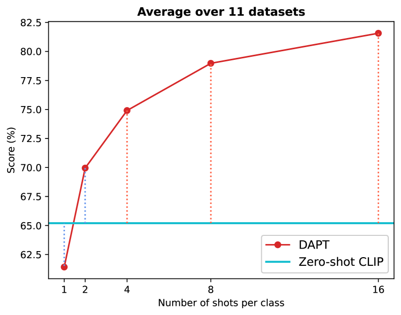
Figure 3: Comparison with Zero-shot CLIP.

Comparison with Linear Probe CLIP. We observed that DAPT shows higher performance than linear probe CLIP for most datasets as noted in Table 2. Especially on OxfordPets [26], DAPT improves the performance by 46.22% with only a single training sample. When comparing all experiments in 1-shot image classification, DAPT achieves an average improvement of 14.87% compared to linear probe CLIP.

Comparison with Zero-Shot CLIP. When comparing DAPT to zero-shot CLIP, DAPT demonstrates higher performance in most experiments, with a similar result to the comparison with linear probe CLIP. Notably, as described in Figure 3, the performance gap between DAPT and zero-shot CLIP widens as the number of samples increases, suggesting that DAPT is adaptive at distribution-aware prompt optimization as the training sample size grows.

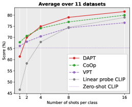
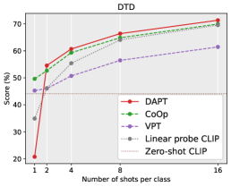
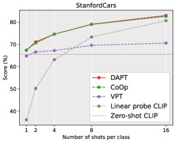
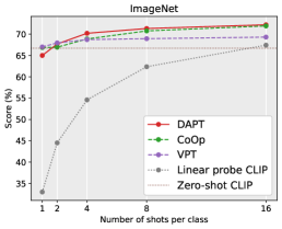
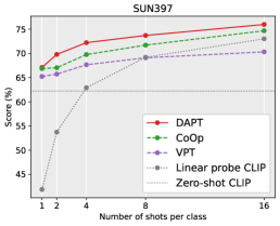
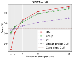
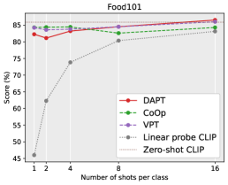
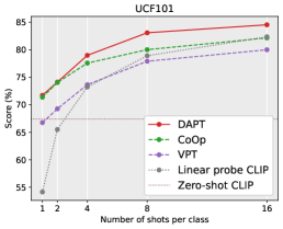
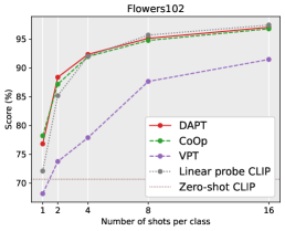
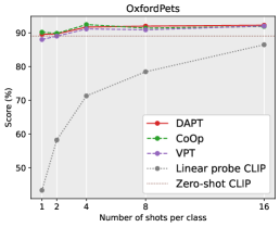
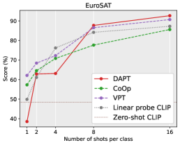
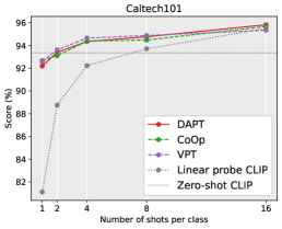
Figure 4: Few-shot learning in image classifications on 11 datasets.

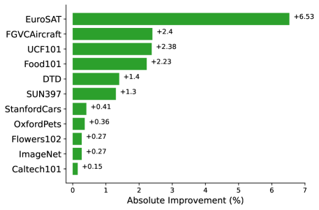
(a)

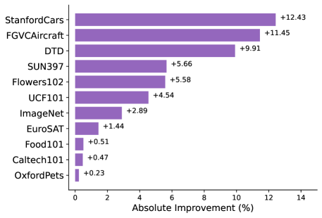
(b)

Figure 5: Comparison with CoOp and VPT. We show the result of image classification with 16 samples from training data per each dataset. Our method has overall improvement compared with CoOp [47] and VPT [16].

Comparison with Previous Prompt Tuning. Figure 5(a) demonstrates the results of DAPT and CoOp [47] on 16 shots. As shown in the results, DAPT outperforms CoOp for all datasets. Furthermore, Figure 5(b) presents the comparison of DAPT and VPT [16] under the same experimental setting. As with the CoOp comparison results, it shows that DAPT outperforms VPT on all datasets, and the accuracy is 12.43% higher than VPT on StanfordCars [19]. To sum up, using DAPT for each modality shows superior performance compared to conventional prompt tuning, as well as zero-shot CLIP and liner probe CLIP.

4.2 Domain Generalization

We evaluate the generalizability of DAPT by comparing it with zero-shot CLIP, and linear probe CLIP in the domain generalization setting. We use ImageNet [5] as a source dataset,and the prompts are trained with 16 samples and the target dataset as ImageNet-R [13], ImageNet-A [14], ImageNetV2 [30], and ImageNet-Sketch [37].

Method	Source	Target
	ImageNet	-V2	-Sketch	-A	-R
Zero-shot CLIP	66.72	60.90	46.10	47.75	73.97
Linear probe CLIP	67.42	57.19	35.97	36.19	60.10
CoOp	71.93	64.22	47.07	48.97	74.32
VPT	69.31	62.36	47.72	46.20	75.81
DAPT	72.20	64.93	48.30	48.74	75.75

Table 3: Comparison on domain generalization.

The overall results are shown in Table 3. From the experimental results, DAPT achieves remarkable performance on unseen data compared to zero-shot CLIP and linear probe CLIP. Compared with CoOp [47] and VPT [16], it slightly decreases accuracy on ImageNet-A and ImageNet-R, respectively. In contrast, in the rest of the dataset, ImageNet-V2 and ImageNet-Sketch, DAPT has superior performance with a significant accuracy gain.

4.3 Ablation Study

Effectiveness of Intra-dispersion Loss and Inter-dispersion Loss. To verify the accuracy improvement when applying the inter-dispersion loss and intra-dispersion loss, we test few-shot learning experiments on 11 datasets with 16 samples from training data. We set the model combined with text prompts, i.e., CoOp [47], and visual prompts, i.e., VPT [16], as a baseline. Table 5 shows the performance improvement of applying inter-dispersion loss and intra-dispersion loss. The experimental results indicate that the accuracy improved overall for 11 datasets and the average of the entire datasets compared to the baseline. As a result, both inter-dispersion loss and intra-dispersion loss show performance gain by reconstructing the embedding space across most datasets. In particular, the inter-dispersion loss and intra-dispersion loss are effective for improving performance on FGVCAircraft [23], and DTD [4], respectively. Interestingly, despite some datasets, i.e., Food101 [2], ImageNet [5], FGVCAircraft [23], Flowers102 [25], and SUN397 [39], slightly decreasing accuracy by adding inter-dispersion loss or intra-dispersion loss, DAPT increases accuracy.

Method	# of training samples in each class
	1	2	4	8	16
CoOp+VPT	61.05	68.49	73.28	78.76	81.25
DAPT	61.42	69.95	74.91	78.98	81.62

Table 4: Ablation study. The average accuracy of CoOp+VPT and DAPT on 11 benchmark datasets is presented.

The results support that reconstructing and optimizing embedding jointly are essential to feature alignment between the modalities. As noted in Table 4, this tendency can also be observed for various shots - DAPT has superior performance compared with the combination of CoOp [47] and VPT [16].

Method	OxfordPets	Flowers102	FGVCAircraft	DTD	EuroSAT	StanfordCars
CoOp+VPT	91.90	96.89	46.06	69.86	91.77	82.78
CoOp+VPT w/ $\mathcal{L}_{\text{inter}}$	91.97	96.85	46.52	70.06	92.01	82.95
CoOp+VPT w/ $\mathcal{L}_{\text{intra}}$	91.97	97.03	45.90	70.76	92.16	83.14
DAPT	92.27	97.06	46.37	71.38	92.65	83.03
Method	Food101	SUN397	Caltech101	UCF101	ImageNet	Average
CoOp+VPT	86.52	75.88	95.70	84.23	72.14	81.25
CoOp+VPT w/ $\mathcal{L}_{\text{inter}}$	86.42	75.71	95.71	84.27	72.07	81.33
CoOp+VPT w/ $\mathcal{L}_{\text{intra}}$	86.47	75.90	95.74	84.35	72.15	81.41
DAPT	86.55	75.99	95.82	84.53	72.20	81.62

Table 5: Abalation study. We compared DAPT with the baseline, i.e., CoOp [47]+VPT [16], on 11 benchmark datasets. We observed performance gain in most datasets by adding losses one by one.

Exploration of Intra-dispersion Loss. As discussed in Section 3, the prototype $\boldsymbol{s}$ is defined as the average of image embeddings in DAPT. To evaluate the prototypes set by the mean of embeddings, we conduct the ablation study of intra-dispersion loss with the prototype (DAPT-R) set by a random sample’s embedding. Table 6 shows the image classification results for 1, 2, 4, 8, and 16-shots on 11 datasets. From the results, we confirmed that clustering around the average of samples (DAPT) is more effective than clustering around the random sample (DAPT-R), especially when the number of shots is not extremely small (i.e., 4, 8, and 16-shots).

Method	# of training samples in each class
	1	2	4	8	16
CoOp+VPT	61.05	68.49	73.28	78.76	81.25
DAPT-R	65.08	70.51	74.85	78.11	81.29
DAPT	61.42	69.95	74.91	78.98	81.62

Table 6: Average performance on 11 datasets. DAPT-R refers to applying intra-dispersion loss $\mathcal{L}_{\text{intra}}$ with the randomly defined prototype.

4.4 Analysis

We investigate whether DAPT learns text and image embeddings as intended - spreading text embeddings and assembling image embeddings within the same classes - by quantitative and qualitative analyses.

Quantitative Analysis. We analyze the pairwise distance pdist and the area of the convex hull of embeddings. Table 7 shows the relative average pairwise distance pdist between image embeddings of the same class compared to zero-shot CLIP, which is computed as the relative ratios, i.e., $\Delta\text{pdist (\%)}=(1-\text{DAPT}/\text{zero-shot CLIP})\times 100$. The results evidence that DAPT properly minimizes the average pairwise distance between image embeddings in a class ($\approx$ intra-dispersion) and maximizes it for text (labels) embeddings across classes ($\approx$ inter-dispersion). This implies that DAPT learns prompts to better latent spaces for feature alignment.

Dataset	Image	Text
	$\Delta\text{pdist}$ (%)	$\Delta\text{pdist}$ (%)	$\text{cvx\_hull}_{\text{text}}$
OxfordPets	0.2	23.4	65.8
Flowers102	-0.3	36.4	145.1
FGVCAircraft	-9.3	62.5	246.4
DTD	-6.4	119.5	713.8
EuroSAT	-22.2	117.1	921.9
StanfordCars	-2.4	30.6	87.8
Food101	-4.6	27.8	115.8
SUN397	-9.9	33.2	148.3
Caltech101	-2.8	45.2	115.3
UCF101	-1.4	51.1	251.4
ImageNet	-0.3	0.2	-12.2

Table 7: Analysis of embeddings from DAPT. Pairwise distances (pdist) and Convex hull area (cvx_hull) of embeddings from DAPT compared to zero-shot CLIP. Ratios, $(1-\text{DAPT}/\text{zero-shot CLIP})\times 100$ are reported.

Qualitative Analysis. We verify that DAPT more compactly clusters image embeddings via t-SNE [36] visualization on several datasets. Figure 6 shows image embeddings of Fowers102 [25] and UCF101 [35] benchmark datasets. Each point represents an image embedding, and the colors of the points indicate their classes. More t-SNE visualizations are provided in the supplement.

Flowers102
UCF101

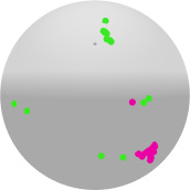
(a)

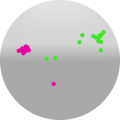
(b)

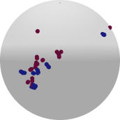
(c)

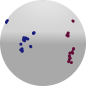
(d)

Figure 6: Visualization of image embeddings. We visualize image embeddings of Flowers102 and UCF101 via t-SNE. Compared to zero-shot CLIP, our DAPT more compactly clusters image embeddings for each class.

5 Limitations and Conclusion

We proposed a distribution-aware prompt tuning method called DAPT for pre-trained vision-language models (VLMs). By considering the distribution of embeddings for prompt-tuning, which is underexplored in the literature, the proposed method significantly improves performance while maintaining the merits of existing prompt-tuning methods. In this paper, we present the inter-dispersion loss and intra-dispersion loss that appropriately optimize the text and visual latent spaces of VLMs, allowing us to achieve higher performance in downstream tasks using only prompts without additional layers. Although the proposed method significantly improves overall performance, it is still challenging to optimize prompts in the extreme few-shot settings, such as 1-shot and 2-shot. Lastly, it will be an interesting future direction to apply it to various downstream applications beyond image classification.

Appendix A Implementation Details

We implement DAPT based on the open source from CoOp [47] and VPT [16], using the PyTorch [27] library. Before training, the learnable vectors for the text prompt are initialized with a zero-mean Gaussian distribution following the CoOp. In contrast, the learnable vectors for the visual prompt are initialized with the Xavier uniform initialization scheme following the VPT. In all experiments, the length of the learnable vector is set to 16 in both the text and visual prompt. In the case of linear probe CLIP [29] and zero-shot CLIP [29], we set the initialization of the text prompt as “a photo of a [CLASS].” In the few-shot learning experiments, we follow the approach of Zhou et al. [47] and conduct random sampling three times for each dataset. We report the average after testing three times for all experiments, including DAPT, CoOp [47], VPT [16], and linear probe CLIP. As observed in the case of VPT, there is variance in the results of the visual prompt depending on hyperparameters such as learning rate. Therefore, we conduct a grid search for learning rate in the range of {0.002, 0.02, 0.2, 2.0, 20.0}, following the approach of Jia et al. [16].

Appendix B Additional Analyses

In this section, we further analyze DAPT with various experiments.

B.1 Analysis of Hyperparameter $\beta_{t}$ and $\beta_{v}$.

The hyperparameter $\beta_{t}$ and $\beta_{v}$ adjust the strength of inter-dispersion loss and intra-dispersion loss, respectively. Due to the characteristics of each dataset, it may have different optimal values. We depict the accuracy according to $\beta_{t}$ and $\beta_{v}$ in Figure 7 to investigate the hyperparameters.

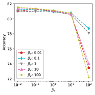
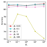
Figure 7: Exploration of hyperparamters.

As described in Figure 7, DAPT shows consistent performance with a wide range of hyperparameters. To sum up, DAPT is robust to the choice of hyperparameters, except $\beta_{t}=100$. Table 10 summarizes optimal hyperparameters for each dataset.

B.2 t-SNE Visualization

Figure 8 presents t-SNE [36] visualization of image embeddings in zero-shot CLIP [29] and DAPT. All plots show that DAPT properly increases the distance between different classes as well as minimizes the intra-class variance. Especially the results on OxfordPets [26], Flowers102 [25], and UCF101 [35] demonstrate that DAPT helps embeddings form compact clusters and increase the distance between different classes.

B.3 Detailed Experimental Results

In all experiments, we ran three times with randomly sampled data in each run and noted average values. For compelling results, we provide accuracy with standard deviation in 16-shots image classification on 11 datasets in Table 8. On average, DAPT achieved the best performance in 10 benchmarks.

Dataset	LP-CLIP	CoOp	VPT	DAPT
OxfordPets	86.49$\pm$0.06	91.91$\pm$0.42	92.04$\pm$0.58	92.27$\pm$0.40
Flowers102	97.51$\pm$0.13	96.79$\pm$0.35	91.48$\pm$0.15	97.06$\pm$0.25
FGVCAircraft	45.51$\pm$0.08	43.96$\pm$0.74	34.92$\pm$0.16	46.37$\pm$1.00
DTD	69.58$\pm$0.73	69.98$\pm$0.18	61.47$\pm$0.37	71.38$\pm$1.62
EuroSAT	87.24$\pm$0.23	85.58$\pm$1.63	90.67$\pm$1.44	92.65$\pm$0.86
StanfordCars	80.67$\pm$0.46	82.62$\pm$0.13	70.59$\pm$1.00	83.03$\pm$0.34
Food101	83.14$\pm$0.45	84.31$\pm$0.17	86.03$\pm$0.27	86.55$\pm$0.10
SUN397	73.03$\pm$0.74	74.69$\pm$0.24	70.33$\pm$0.16	75.99$\pm$0.12
Caltech101	95.51$\pm$0.31	95.68$\pm$0.20	95.35$\pm$0.15	95.82$\pm$0.07
UCF101	82.35$\pm$0.36	82.15$\pm$1.42	79.99$\pm$0.69	84.53$\pm$0.55
ImageNet	67.42$\pm$0.26	71.93$\pm$0.10	69.31$\pm$0.05	72.20$\pm$0.18

Table 8: 16-shots image classification on 11 datasets.

Appendix C Generalization From Base to New Classes

CoOp [47] demonstrated exemplary performance in the few-shot learning using text prompts, but it has a weak generalizability problem regarding unseen classes, as discussed in CoCoOp [46]. As shown in Table 2, we prove that DAPT has significant performance gain in generalization. However, we supplement more experiments to prove that DAPT has superior generalization performance compared with baselines. In all experiments, we evaluate not only original classes but also unseen classes. Following Zhou et al. [46], we divide the dataset into base classes and new classes, then train on 16 samples of the base class before testing on the new class. Similarly to the few-shot learning setting, we report the average of three times. The result for 11 datasets and the overall average is presented in Table 9. The experimental results show that the accuracy for the new class is higher than CoOp in most datasets. The harmonic mean of the base and new class demonstrates superior performance for seven datasets.

(a) OxfordPets [26].		(b) Flowers102 [25].
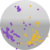
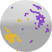
(c) DTD [4].		(d) StanfordCars [19].
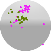
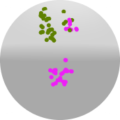
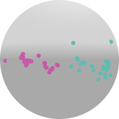
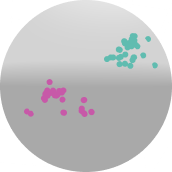
(e) FGVCAircraft [23].		(f) Caltech101 [8].
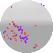
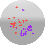
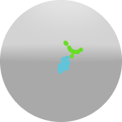
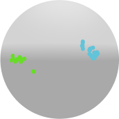
(e) UCF101 [35].		(i) EuroSAT [12].

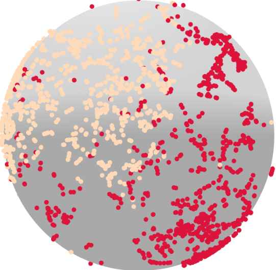
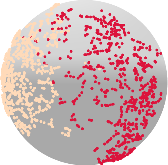
Figure 8: t-SNE [36] visualization of image embeddings. In each dataset, the left hypersphere represents zero-shot CLIP, and the right hypersphere represents DAPT.

(a) Average over 11 datasets. Base New H CLIP 69.53 74.34 71.85 CoOp 82.71 62.84 71.42 DAPT 84.20 63.71 72.54	(b) OxfordPets [26]. Base New H CLIP 91.33 97.15 94.15 CoOp 93.37 95.43 94.39 DAPT 94.00 72.43 81.82	(c) Flowers102 [25]. Base New H CLIP 71.70 77.45 74.46 CoOp 97.82 59.79 74.21 DAPT 98.16 61.37 75.53
(d) FGVCAircraft [23]. Base New H CLIP 27.67 35.87 31.24 CoOp 40.66 24.44 30.53 DAPT 45.54 19.74 27.54	(e) DTD [4]. Base New H CLIP 53.24 60.87 56.80 CoOp 79.59 40.30 53.51 DAPT 82.06 53.42 64.71	(f) EuroSAT [12]. Base New H CLIP 56.93 63.92 60.22 CoOp 92.21 50.70 65.43 DAPT 95.05 43.02 59.23
(g) StanfordCars [19]. Base New H CLIP 63.93 74.99 69.02 CoOp 77.70 59.39 67.32 DAPT 79.69 57.46 66.77	(h) Food101 [2]. Base New H CLIP 90.08 91.13 90.60 CoOp 88.40 85.87 87.11 DAPT 89.57 89.82 89.69	(i) SUN397 [39]. Base New H CLIP 69.46 75.56 72.38 CoOp 80.64 65.43 72.24 DAPT 81.87 74.80 78.18
(j) Caltech101 [8]. Base New H CLIP 97.22 94.21 95.69 CoOp 98.19 86.17 91.79 DAPT 98.24 87.74 92.69	(k) UCF101 [35]. Base New H CLIP 70.89 78.42 74.47 CoOp 84.80 55.62 67.17 DAPT 85.09 71.46 77.68	(l) ImageNet [5]. Base New H CLIP 72.40 68.12 70.19 CoOp 76.44 68.11 72.04 DAPT 76.97 69.54 73.07

Table 9: Comparison of CLIP, CoOp, and DAPT in the base-to-new generalization setting.

Hyperparameters	OxfordPets	Flowers102	FGVCAircraft	DTD	EuroSAT	StanfordCars	Food101	SUN397	Caltech101	UCF101	ImageNet
$\beta_{t}$	0.1	0.01	0.01	0.01	10.0	0.1	0.01	0.01	0.01	0.1	0.01
$\beta_{v}$	10.0	10.0	100.0	100.0	100.0	100.0	10.0	100.0	10.0	0.1	0.01
Learning rate	0.02	0.002	2.0	20.0	20.0	0.002	20.0	20.0	0.2	20.0	2.0

Table 10: Hyperparameters on 11 datasets in few-shot learning.

References

- [1] Hyojin Bahng, Ali Jahanian, Swami Sankaranarayanan, and Phillip Isola. Visual prompting: Modifying pixel space to adapt pre-trained models. arXiv preprint arXiv:2203.17274, 2022.
- [2] Lukas Bossard, Matthieu Guillaumin, and Luc Van Gool. Food-101–mining discriminative components with random forests. In ECCV, 2014.
- [3] Guangyi Chen, Weiran Yao, Xiangchen Song, Xinyue Li, Yongming Rao, and Kun Zhang. Prompt learning with optimal transport for vision-language models. In ICLR, 2023.
- [4] Mircea Cimpoi, Subhransu Maji, Iasonas Kokkinos, Sammy Mohamed, and Andrea Vedaldi. Describing textures in the wild. In CVPR, 2014.
- [5] Jia Deng, Wei Dong, Richard Socher, Li-Jia Li, Kai Li, and Li Fei-Fei. Imagenet: A large-scale hierarchical image database. In CVPR, 2009.
- [6] Alexey Dosovitskiy, Lucas Beyer, Alexander Kolesnikov, Dirk Weissenborn, Xiaohua Zhai, Thomas Unterthiner, Mostafa Dehghani, Matthias Minderer, Georg Heigold, Sylvain Gelly, Jakob Uszkoreit, and Neil Houlsby. An image is worth 16x16 words: Transformers for image recognition at scale. In ICLR, 2021.
- [7] Yu Du, Fangyun Wei, Zihe Zhang, Miaojing Shi, Yue Gao, and Guoqi Li. Learning to prompt for open-vocabulary object detection with vision-language model. In CVPR, 2022.
- [8] Li Fei-Fei, Rob Fergus, and Pietro Perona. Learning generative visual models from few training examples: An incremental bayesian approach tested on 101 object categories. In CVPRW, 2004.
- [9] Noa Garcia, Mayu Otani, Chenhui Chu, and Yuta Nakashima. Knowit vqa: Answering knowledge-based questions about videos. In AAAI, 2020.
- [10] Shashank Goel, Hritik Bansal, Sumit Bhatia, Ryan Rossi, Vishwa Vinay, and Aditya Grover. Cyclip: Cyclic contrastive language-image pretraining. In NeurIPS, 2022.
- [11] Xiuye Gu, Tsung-Yi Lin, Weicheng Kuo, and Yin Cui. Open-vocabulary object detection via vision and language knowledge distillation. In ICLR, 2022.
- [12] Patrick Helber, Benjamin Bischke, Andreas Dengel, and Damian Borth. Eurosat: A novel dataset and deep learning benchmark for land use and land cover classification. IEEE Journal of Selected Topics in Applied Earth Observations and Remote Sensing, 2019.
- [13] Dan Hendrycks, Steven Basart, Norman Mu, Saurav Kadavath, Frank Wang, Evan Dorundo, Rahul Desai, Tyler Zhu, Samyak Parajuli, Mike Guo, et al. The many faces of robustness: A critical analysis of out-of-distribution generalization. In ICCV, 2021.
- [14] Dan Hendrycks, Kevin Zhao, Steven Basart, Jacob Steinhardt, and Dawn Song. Natural adversarial examples. In CVPR, 2021.
- [15] Chao Jia, Yinfei Yang, Ye Xia, Yi-Ting Chen, Zarana Parekh, Hieu Pham, Quoc Le, Yun-Hsuan Sung, Zhen Li, and Tom Duerig. Scaling up visual and vision-language representation learning with noisy text supervision. In ICML, 2021.
- [16] Menglin Jia, Luming Tang, Bor-Chun Chen, Claire Cardie, Serge Belongie, Bharath Hariharan, and Ser-Nam Lim. Visual prompt tuning. In ECCV, 2022.
- [17] Zhengbao Jiang, Frank F Xu, Jun Araki, and Graham Neubig. How can we know what language models know? ACL, 2020.
- [18] Muhammad Uzair khattak, Hanoona Rasheed, Muhammad Maaz, Salman Khan, and Fahad Shahbaz Khan. Maple: Multi-modal prompt learning. In CVPR, 2023.
- [19] Jonathan Krause, Michael Stark, Jia Deng, and Li Fei-Fei. 3d object representations for fine-grained categorization. In ICCVW, 2013.
- [20] Brian Lester, Rami Al-Rfou, and Noah Constant. The power of scale for parameter-efficient prompt tuning. In EMNLP, 2021.
- [21] Junnan Li, Dongxu Li, Silvio Savarese, and Steven Hoi. BLIP-2: bootstrapping language-image pre-training with frozen image encoders and large language models. In ICML, 2023.
- [22] Yuning Lu, Jianzhuang Liu, Yonggang Zhang, Yajing Liu, and Xinmei Tian. Prompt distribution learning. In CVPR, 2022.
- [23] S. Maji, J. Kannala, E. Rahtu, M. Blaschko, and A. Vedaldi. Fine-grained visual classification of aircraft. Technical report, 2013.
- [24] Ron Mokady, Amir Hertz, and Amit H Bermano. Clipcap: Clip prefix for image captioning. arXiv preprint arXiv:2111.09734, 2021.
- [25] Maria-Elena Nilsback and Andrew Zisserman. Automated flower classification over a large number of classes. In ICVGIP, 2008.
- [26] Omkar M Parkhi, Andrea Vedaldi, Andrew Zisserman, and CV Jawahar. Cats and dogs. In CVPR, 2012.
- [27] Adam Paszke, Sam Gross, Soumith Chintala, Gregory Chanan, Edward Yang, Zachary DeVito, Zeming Lin, Alban Desmaison, Luca Antiga, and Adam Lerer. Automatic differentiation in pytorch. 2017.
- [28] Fabio Petroni, Tim Rocktäschel, Patrick Lewis, Anton Bakhtin, Yuxiang Wu, Alexander H Miller, and Sebastian Riedel. Language models as knowledge bases? In EMNLP, 2019.
- [29] Alec Radford, Jong Wook Kim, Chris Hallacy, Aditya Ramesh, Gabriel Goh, Sandhini Agarwal, Girish Sastry, Amanda Askell, Pamela Mishkin, Jack Clark, et al. Learning transferable visual models from natural language supervision. In ICML, 2021.
- [30] Benjamin Recht, Rebecca Roelofs, Ludwig Schmidt, and Vaishaal Shankar. Do imagenet classifiers generalize to imagenet? In ICML, 2019.
- [31] Sheng Shen, Shijia Yang, Tianjun Zhang, Bohan Zhai, Joseph E Gonzalez, Kurt Keutzer, and Trevor Darrell. Multitask vision-language prompt tuning. arXiv preprint arXiv:2211.11720, 2022.
- [32] Taylor Shin, Yasaman Razeghi, Robert L Logan IV, Eric Wallace, and Sameer Singh. Autoprompt: Eliciting knowledge from language models with automatically generated prompts. In EMNLP, 2020.
- [33] Amanpreet Singh, Ronghang Hu, Vedanuj Goswami, Guillaume Couairon, Wojciech Galuba, Marcus Rohrbach, and Douwe Kiela. FLAVA: A foundational language and vision alignment model. In CVPR, 2022.
- [34] Jake Snell, Kevin Swersky, and Richard Zemel. Prototypical networks for few-shot learning. In NeurIPS, 2017.
- [35] Khurram Soomro, Amir Roshan Zamir, and Mubarak Shah. Ucf101: A dataset of 101 human actions classes from videos in the wild. arXiv preprint arXiv:1212.0402, 2012.
- [36] Laurens Van der Maaten and Geoffrey Hinton. Visualizing data using t-sne. JMLR, 2008.
- [37] Haohan Wang, Songwei Ge, Zachary Lipton, and Eric P Xing. Learning robust global representations by penalizing local predictive power. In NeurIPS, 2019.
- [38] Tongzhou Wang and Phillip Isola. Understanding contrastive representation learning through alignment and uniformity on the hypersphere. In ICML, 2020.
- [39] Jianxiong Xiao, James Hays, Krista A Ehinger, Aude Oliva, and Antonio Torralba. Sun database: Large-scale scene recognition from abbey to zoo. In CVPR, 2010.
- [40] Lu Yuan, Dongdong Chen, Yi-Ling Chen, Noel Codella, Xiyang Dai, Jianfeng Gao, Houdong Hu, Xuedong Huang, Boxin Li, Chunyuan Li, et al. Florence: A new foundation model for computer vision. arXiv preprint arXiv:2111.11432, 2021.
- [41] Yuhang Zang, Wei Li, Kaiyang Zhou, Chen Huang, and Chen Change Loy. Unified vision and language prompt learning. arXiv preprint arXiv:2210.07225, 2022.
- [42] Renrui Zhang, Jiaming Han, Chris Liu, Peng Gao, Aojun Zhou, Xiangfei Hu, Shilin Yan, Pan Lu, Hongsheng Li, and Yu Qiao. Llama-adapter: Efficient fine-tuning of language models with zero-init attention. arXiv preprint arXiv:2303.16199, 2023.
- [43] Yuhao Zhang, Hang Jiang, Yasuhide Miura, Christopher D Manning, and Curtis P Langlotz. Contrastive learning of medical visual representations from paired images and text. In MLHC, 2022.
- [44] Yiwu Zhong, Jianwei Yang, Pengchuan Zhang, Chunyuan Li, Noel Codella, Liunian Harold Li, Luowei Zhou, Xiyang Dai, Lu Yuan, Yin Li, et al. Regionclip: Region-based language-image pretraining. In CVPR, 2022.
- [45] Chong Zhou, Chen Change Loy, and Bo Dai. Extract free dense labels from clip. In ECCV, 2022.
- [46] Kaiyang Zhou, Jingkang Yang, Chen Change Loy, and Ziwei Liu. Conditional prompt learning for vision-language models. In CVPR, 2022.
- [47] Kaiyang Zhou, Jingkang Yang, Chen Change Loy, and Ziwei Liu. Learning to prompt for vision-language models. IJCV, 2022.