Sources of capital growth

Abstract

Data from national accounts show no effect of change in net saving or consumption, in ratio to market-value capital, on change in growth rate of market-value capital (capital acceleration). Thus it appears that capital growth and acceleration arrive without help from net saving or consumption restraint. We explore ways in which this is possible, and discuss implications for economic teaching and public policy.

1 Introduction and overview

Many economists over the centuries have reasoned that net saving, or equivalently net investment, should tend to give equal capital growth. Economists since the early nineteenth century have added the proviso that net saving cannot safely outpace innovation; more capital must mean capital redesigned for greater productivity if economies are to escape risk of capital glut and diminishing returns (West (1815), Ricardo (1815), Malthus (1815)). Roy Harrod (1939) described that limit for safe net saving, meaning the rate of imagining and developing new ideas for more productive forms of capital, as the “warranted rate”. Harrod, and many other economists of his time and since, have focused on growth of output rather than of capital, but have modeled growth of output by first assuming the equivalence of net saving and capital growth, within the warranted rate, and then looking for effects of that capital growth on later output growth.

Some other economists, including John Rae (1834) and John Stuart Mill (1848), argued that capital growth might also be explained by a rise in productivity of capital and labor already in place. Ways might found for existing factors to produce more, that is, and so to allow more consumption, or more capital growth, or any mix of the two, without inputs of net saving. Robert Solow (1957), allowed that possibility for “disembodied” growth, where plant and products already existing are repurposed or redeployed in more productive ways.

We test between those two explanations of capital growth, by net saving or by increase in productivity of capital and labor already in place, by comparing net saving to concurrent change in market-value capital in 88 countries. As changes in net saving are expected to be associated with opposite changes in consumption, we also compare change in consumption to concurrent change in capital growth (capital acceleration). All data are drawn from national accounts of those countries as collated on the free website World Inequality Database.

Tests show no effect of net saving or of change in consumption on growth or acceleration of market-value capital. These findings support the views of Rae and Mill, and of Solow as to disembodied growth. They suggest that capital growth, even in acceleration, arrives without help from net saving or consumption restraint. Net saving, if so, raises the physical quantity of capital, but not the aggregate value, and so reduces the value per unit.

Our findings are most easily explained by the present value principle, and by production efficiencies enabled through innovation. Value is created in the mind of the market at the moment when prospective cash flows are discounted. It is created only if the market sees a path, step by step, from the start, to practical realization of those prospective cash flows. Then capital growth arrives when the market first evaluates prospective cash flows, and is realized eventually in physical outcomes insofar as the market has predicted correctly. Meanwhile the innovator acquires materials and plant capacity and labor skills at market prices determined by their uses in current technology, but applies them more productively until competition catches up. It is that temporary market advantage to the innovator which explains capital growth without net saving in a practical and mechanical sense, while the present value principle gives the explanation in terms of market valuation. This idea will be called “free growth theory” for easy reference.

It predicts only at the largest scales, and only for the private sector. Individuals and groups and even small economies can grow through investment from outside. That possibility is foreclosed only at the scale of all capital and all economies together. The public sector, meanwhile, responds to political rather than market choices, and grows or shrinks accordingly.

If free growth theory is right, tax policy and other policy to encourage saving over consumption should be reconsidered. These policies include the higher tax on ordinary income than on capital gains, and the double tax on corporate dividends.

Inferences for economic teaching include the obvious ones for growth theory and for net saving in general. They include others as well. One of the central doctrines of the marginalist revolution has held that market realization converges to producer cost, when that cost includes imputed interest on assets owned. Net saving gives producer cost, and falls short of market realization in the presence of technological growth from new ideas. Meanwhile the doctrine that net income equals consumption plus net saving is put into question by evidence offered here suggesting that net saving increases the physical quantity of capital, but not the aggregate value. In general, economics might consider relying less on book value, and more on market value and on the power of ideas.

2 Net saving and capital growth

This study compares net saving $S_{net}$ to concurrent growth in market-value capital $K$ from data in national accounts. Capital growth ${\Delta K}_{i}$ in each year $i$ for each reporting country is found as $K_{i}-K_{i-1},$ and compared to $S_{net,i}$ reported for that year and country. As we will be testing for differences between $\Delta K$ and $S_{net,i}$, we begin by writing

$$\hypertarget{eq-1}{}{\Delta K_{i}=S_{net,i}+Q_{i}\ ,}$$ (1)

where $Q_{i}$ will mean the sum of market noise, which may prove positive or negative or zero, plus any part of capital growth explained by concurrent productivity gain as described by Rae and Mill, and by Solow as to disembodied growth. We call this sum of noise and productivity gain “free growth” in that it costs no net saving.

The object of testing is to find effects of $S_{net}$ on concurrent $\Delta K$, and so to help evaluate historic and current teachings as to those effects. We submitted above that most teaching, with exceptions noted as to Rae, Mill, and Solow, and within the warranted rate, predicts net saving to differ from concurrent growth in market-value capital only by market noise which tends to balance out over scale and time. The residual term $Q$ in Eq. (1), in that case, will give the market noise converging to zero. That consensus prediction, which we will challenge, will here be called “thrift theory”; $S_{net}$, in thrift theory, is expected to converge to $\Delta K$ if held within the warranted rate. That is,

$$\hypertarget{eq-2}{}{E(\Delta K)=S_{net}\quad\text{or equivalently}\quad E(Q)=0,\quad\text{if}\quad\frac{\Sigma S_{net}}{\Sigma K}\leq u\ ,\quad\text{in thrift theory,}}$$ (2)

where:

1. $\Sigma S_{net}$ is collective net saving over the economy

2. $\Sigma K$ is collective capital over the economy before current $\Sigma S_{net},$ and

3. $u$ is the warranted rate.

$E(\Delta K)$ and $E(Q)$ here give the expected values of $\Delta K$ and $Q$ respectively. Expected value means predicted average of outcomes over all observations. In this case, that will mean predicted average of yearly observations over all years reported. As secular economic growth has tended to make later stocks and flows larger than earlier ones, we first divide by $K$ (normalize) to avoid overweighting of more recent years in finding that average. Division of Eq. (1) by $K_{i-1}$ gives

$$\hypertarget{eq-3}{}{\frac{{\Delta K}_{i}}{K_{i-1}}=\frac{S_{net,i}}{K_{i-1}}+\frac{Q_{i}}{K_{i-1}}\ .}$$ (3)

The first term in Eq. (3) gives capital growth rate $g(K)$. The second term is a variant of the Keynesian net saving rate $s_{net}$ where capital rather than output becomes the denominator. This flow will here be called “thrift”. It will show as $s(K)$, with the subscript “net” left implicit, and with the understanding that the denominator shows capital at market value, rather than at depreciated cost. The third term in Eq. (3) will be called free growth rate and shown as $q(K)$. Then

$$g{(K)}_{i}=\frac{\Delta K_{i}}{K_{i-1}}\ ,\quad s{(K)}_{i}=\frac{S_{net,i}}{K_{i-1}}\ ,\quad\text{and}\quad q{(K)}_{i}=\frac{Q_{i}}{K_{i-1}}\ ,$$

so that Eq. (3) can be shown more compactly as

$$\hypertarget{eq-3a}{}{g{(K)}_{i}=s{(K)}_{i}+{q(K)}_{i}\ .}$$ (4)

By the definition $q(K)=\frac{Q}{K}$, an expected value $E(Q)=0$ implies $E\left(q(K)\right)=0$. Application of Eq. (2) to Eq. (4) now gives

$$\hypertarget{eq-4}{}{E\left(g(K)\right)=s{(K)}\quad\text{and}\quad E(q(K))=0\ ,\quad\text{under thrift assumptions,}}$$ (5)

where “thrift assumptions” are that thrift theory is correct and that the warranted rate is not exceeded. Meanwhile Eq. (4) allows

$$\hypertarget{eq-5}{}{\Delta g{(K)}_{i}=\Delta s{(K)}_{i}+\Delta q{(K)}_{i}\ ,\quad\text{where}}$$ (6)

$$\Delta g{(K)}_{i}=g{(K)}_{i}-g(K)_{i-1}\ ,\quad\Delta s(K)_{i}=s(K)_{i}-s(K)_{i-1}\ ,\quad\text{and}\quad\Delta q{(K)}_{i}=q{(K)}_{i}-q{(K)}_{i-1}\ .$$

For any variables $a$ and $b$, we may reason $E(a-b)=E(a)-E(b)$. By this and by Eqs. (5) and (6), then,

$$\hypertarget{eq-6}{}{E\left(\Delta g(K)\right)=E\left(\Delta s(K)\right)\quad\text{and}\quad E(\Delta q(K))=0\ ,\quad\text{under thrift assumptions.}}$$ (7)

The first term in Eq. (6) may be called “capital acceleration”. Division of Eq. (6) by capital acceleration, and rearrangement, gives

$$\hypertarget{eq-7}{}{\frac{\Delta s{(K)}_{i}}{\Delta g{(K)}_{i}}+\frac{\Delta q{(K)}_{i}}{\Delta g{(K)}_{i}}=1\ .}$$ (8)

Define $\theta_{s,i}=\frac{\Delta s{(K)}_{i}}{\Delta g{(K)}_{i}}$ and $\varphi_{s,i}=\frac{\Delta q{(K)}_{i}}{\Delta g{(K)}_{i}}$ to restate Eq. (8) as

$$\hypertarget{eq-7a}{}{\theta_{s,i}+\varphi_{s,i}=1\ .}$$ (9)

Next define $\theta_{s}=E(\theta_{s,i})$ and $\varphi_{s}=E(\varphi_{s,i})$. By Eq. (9), then,

$$\theta_{s}+\varphi_{s}=1\ .\quad\text{Eq. \eqref{eq-6} now implies}$$ (10)

$$\theta_{s}=1\quad\text{and}\quad\varphi_{s}=0\ ,\quad\text{under thrift assumptions.}$$ (11)

$\theta$ and $\varphi$ will be called the “thrift index” and “free growth index” respectively. $\theta_{s}$ and $\varphi_{s}$ give their values as found from data for net saving. Expected values, again, are predicted averages of outcomes. Thus Eq. (11) and thrift theory can be tested by finding average values of $\theta_{s,i}$ and comparing findings to the expected value $\theta=1$. First we find

$$\overline{\theta_{s,i}}=\frac{1}{m}\sum^{m}\theta_{s,i}\quad\text{and}\quad\overline{\varphi_{s,i}}=\frac{1}{m}\sum^{m}\varphi_{s,i}\ ,$$

where $m$ is the number of observed values of $\theta_{s,i}$ and $\varphi_{s,i}$, and test the predictions

$$\overline{\theta_{s,i}}\cong 1\quad\text{and}\quad\overline{\varphi_{s,i}}\cong 0\ .$$

Calculations of $\overline{\theta_{s,i}}$ and $\overline{\varphi_{s,i}}$ are not expected to show 1 and 0 exactly, under thrift assumptions, because the number of samples $m$ is finite.

Fig. 1 shows average values of $\theta_{s}$ and $\varphi_{s}$ for 88 countries, both unweighted and weighted to GDP, over the period 1980-2022. To control distortions brought by small absolute denominators, years were screened out where $|\Delta g(K)|$ was found at less than 0.01 (see Section 9). Results show $\varphi_{s}\cong 1$ and $\theta_{s}\cong 0$. These findings appear to refute thrift theory, and to support free growth theory as defined earlier. $Q$, predicted in thrift theory to describe effects of market noise converging to zero, is revealed to include also the effects of productivity gain as described by Rae, Mill and Solow. We will now test thrift theory from a different approach.

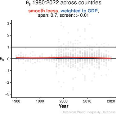
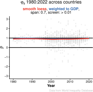
Fig. 1: Thrift and free growth indexes derived from net saving (88 countries).

Table 1: Regression of $\Delta g(K)$ to value shown (Screen = 0.01). $H_{0}\ \text{per thrift theory:}\ \theta_{s}=1\ \&\ \varphi_{s}=0$

	$\theta_{s}$	$\varphi_{s}$
Regression of $\Delta g(K)$ to value shown	0.3232∗∗∗	0.6768∗∗∗
	(0.1903)	(0.1903)
Observations	1,414	1,414
R2	0.30255	0.65196
Within R2	0.28611	0.63734
Year fixed effects	$\checkmark$	$\checkmark$
Country fixed effects	$\checkmark$	$\checkmark$

3 Consumption and capital growth

By analogy to Eq. (1), write

$$\hypertarget{eq-10}{}{\Delta K_{i}+C_{i}=Z_{i}\quad\text{or equivalently}\quad\Delta K_{i}=Z_{i}-C_{i}\ ,}$$ (12)

where $C$ gives consumption.

In national accounts, which do not recognize human capital and which measure the worker’s contribution to net output in pay received, $Z$ as defined in Eq. (12) gives net output $Y$. Net output is defined as value added. Reckoning in terms of human capital could suggest that the sum of $C$ and $\Delta K$ misses the contribution of self-invested work to value added, and forgets to subtract human depreciation. An Appendix will present an argument that true net output is that sum with these two corrections. Meanwhile we may suspend judgment as to the meaning of $Z$, and take it only as the sum of $\Delta K$ and $C$.

If net saving $S_{net}$ is available only through equal decrease in consumption $-C$, then (2) and (12) give

$$E(\Delta K)=-C\quad\text{and}\quad E(Z)=0\ ,\quad\text{under thrift assumptions.}$$ (13)

We see that Eq. (13) might conflict with the teaching of the possibility of balanced growth, where capital, consumption, output and other flows all grow at the same constant rate. Thus thrift theory, which is meant to reflect what is actually taught, does so with that reservation here and through Eq. (23) below. Continuing as before, anyhow, we divide Eq. (12) by market-value capital to get

$$\hypertarget{eq-11}{}{\frac{\Delta K_{i}}{K_{i-1}}=\frac{Z_{i}}{K_{i-1}}-\frac{C_{i}}{K_{i-1}}\ .}$$ (14)

The expression $C_{i}/K_{i-1}$ in Eq. (14) is a version of the Keynesean consumption rate $c$, but again where market-value capital rather than output is the denominator. It can show as $c(K)$. The second term in Eq. (14) can be notated $z(K)$. By Eq. (14), then,

$$\hypertarget{eq-11a}{}{g(K)_{i}=z(K)_{i}-c(K)_{i}\ .}$$ (15)

By Eqs. (13) and (15), also,

$$E\left(g(K)\right)=-c(K)\quad\text{and}\quad E\left(z(K)\right)=0\ ,\quad\text{under thrift assumptions.}$$ (16)

Eq. (15) meanwhile allows

$$\hypertarget{eq-12}{}{\Delta g(K)_{i}=\Delta z(K)_{i}-\Delta c(K)_{i}\ ,\quad\text{where}}$$ (17)

$$\Delta g(K)_{i}=g(K)_{i}-g(K)_{i-1}\ ,\quad\Delta zK_{i}=z(K)_{i}-z(K)_{i-1}\ ,\quad\text{and}\quad\Delta c(K)_{i}=c(K)_{i}-c(K)_{i-1}\ ,\quad\text{as before.}$$

From Eqs. (16) and (17), then,

$$E\left(\Delta g(K)\right)=E\left(-\Delta c(K)\right)\quad\text{and}\quad E\left(\Delta z(K)\right)=0\ ,\quad\text{under thrift assumptions.}$$ (18)

Now divide Eq. (17) by $\Delta g(K)_{i}$, and rearrange as before, to reach

$$\hypertarget{eq-14}{}{\frac{\Delta z(K)_{i}}{\Delta g(K)_{i}}+\frac{-\Delta c(K)_{i}}{\Delta g(K)_{i}}=1\ .}$$ (19)

Define $\theta_{c,i}=\frac{-\Delta c{(K)}_{i}}{\Delta g(K)_{i}}$ and $\varphi_{c,i}=\frac{\Delta z{(K)}_{i}}{\Delta g(K)_{i}}$ to re-express Eq. (19) as

$$\hypertarget{eq-14a}{}{\theta_{c,i}+\varphi_{c,i}=1\ .}$$ (20)

By Eqs. (18), (19) and (20), further,

$$\hypertarget{eq-15}{}{E\left(\theta_{c,i}\right)=1\quad\text{and}\quad E\left(\varphi_{c,i}\right)=0\ ,\quad\text{under thrift assumptions.}}$$ (21)

Define $\theta_{c}=E\left(\theta_{c,i}\right)$ and $\varphi_{c}=E\left(\varphi_{c,i}\right)$ to re-express Eqs. (20) and (21) respectively as

$$\theta_{c}+\varphi_{c}=1\ ,\quad\text{and}$$ (22)

$$\theta_{c}=1\quad\text{and}\quad\varphi_{c}=0\ ,\quad\text{under thrift assumptions.}$$ (23)

We infer $\theta_{c}\cong\overline{\theta_{c,i}}$ and $\varphi_{c}\cong\overline{\varphi_{c,i}}$ as before, and test thrift theory by comparing average yearly values of $\theta_{c,i}$ and $\varphi_{c,i}$ to its predictions $\overline{\theta_{c,i}}\cong 1$ and $\overline{\varphi_{c,i}}\cong 0$.

Fig. 2 shows results of tests of these predictions from data for consumption reported in national accounts. Consumption was measured as the sum of personal consumption expenditure PCE and government consumption expenditure GCE. Capital K was again measured at market value. Again, years showing $|\Delta g(K)|<.01$ were screened out to control small denominator effects. Test results show $\varphi_{c}\cong 1$ and $\theta_{c}\cong 0$, as with tests for $\varphi_{s}$ and $\theta_{s}$ from net saving. Table 3, which shows $\varphi_{s}$ and $\varphi_{c}$ for the same 88 countries separately, likewise finds $\varphi_{s}\cong 1$ and $\varphi_{c}\cong 1$. Thus it appears that capital acceleration arrives without help from either net saving or consumption restraint. Next we will see how these findings for $\varphi_{s}$ and $\varphi_{c}$ might be explained.

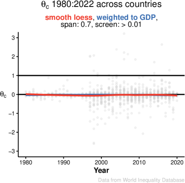
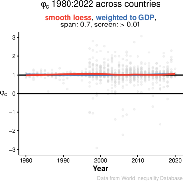
Fig. 2: Thrift and free growth indexes derived from consumption (88 countries).

Table 2: Regression of $\Delta g(K)$ to $\theta_{c}$ and $\varphi_{c}$ (Screen = 0.01). $H_{0}\ \text{per thrift theory:}\ \theta_{c}=1\ \&\ \varphi_{c}=0$

	$\theta_{c}$	$\varphi_{c}$
Regression of $\Delta g(K)$ to value shown	-0.9593∗∗∗	1.959∗∗∗
	(0.0387)	(0.0387)
Observations	1,598	1,598
R2	0.94432	0.98599
Within R2	0.93871	0.98459
Year fixed effects	$\checkmark$	$\checkmark$
Country fixed effects	$\checkmark$	$\checkmark$

Table 3: Average $\varphi_{s,i}$ and $\varphi_{c,i}$ in all countries (screen = 0.01). Number of years clearing screen shown in ()

Country Period $\overline{\varphi_{s,i}}$ $\overline{\varphi_{c,i}}$ Armenia 1997 - 2018 (17) 0.95 1.00 Aruba 1997 - 2001 (5) 0.77 2.02 Australia 1962 - 2019 (43) 0.97 1.01 Austria 1997 - 2017 (14) 0.92 1.03 Azerbaijan 1997 - 2018 (20) 0.67 1.08 Bahrain 2010 - 2013 (4) 0.61 1.03 Belgium 1997 - 2011 (10) 0.89 1.01 Bolivia 1998 - 2013 (13) 1.00 1.03 Botswana 1997 - 2000 (4) 0.75 1.10 Brazil 1998 - 2017 (16) 0.86 1.02 British Virgin Islands 1997 - 1999 (3) 0.11 1.62 Bulgaria 1997 - 2017 (15) 0.99 1.03 Burkina Faso 2001 - 2018 (14) 0.98 0.98 Cabo Verde 2009 - 2016 (8) 0.52 0.95 Cameroon 1998 - 2003 (5) 1.11 0.92 Canada 1974 - 2020 (37) 0.89 0.97 Chile 1998 - 2018 (16) 0.88 1.02 China 1993 - 2014 (20) 0.97 1.03 Colombia 1997 - 2018 (19) 0.91 1.10 Costa Rica 2014 - 2017 (4) 0.97 1.04 Cote d’Ivoire 1997 - 2000 (4) 0.98 1.59 Croatia 1997 - 2019 (18) 0.90 1.05 Curacao 2002 - 2016 (12) 0.94 1.11 Cyprus 1998 - 2019 (18) 0.91 1.05 Czech Republic 1995 - 2015 (14) 1.04 1.04 Denmark 1997 - 2020 (21) 0.91 0.97 Dominican Republic 2007 - 2016 (9) 0.77 1.10 Ecuador 2009 - 2018 (9) 0.66 0.84 Egypt 1998 - 2015 (17) 0.80 0.95 Estonia 1997 - 2019 (17) 0.96 1.02 Finland 1998 - 2020 (18) 0.97 1.03 France 1952 - 2018 (38) 0.87 1.02 Germany 1972 - 2020 (26) 0.89 1.01 Greece 1996 - 2019 (19) 0.90 1.04 Guatemala 2003 - 2019 (9) 0.91 1.02 Guinea 2005 - 2010 (5) 0.92 1.13 Honduras 2003 - 2015 (13) 0.80 0.97 Hong Kong 1997 - 2020 (21) 0.91 1.03 Hungary 1997 - 2019 (18) 0.94 1.06 Iceland 2003 - 2014 (12) 0.87 1.02 India 2000 - 2017 (13) 0.84 0.98 Iran 1997 - 2018 (21) 0.14 0.98 Ireland 1997 - 2019 (19) 0.94 0.99 Israel 1997 - 2018 (19) 0.98 1.17 Country Period $\overline{\varphi_{s,i}}$ $\overline{\varphi_{c,i}}$ Italy 1981 - 2020 (28) 0.93 1.01 Japan 1981 - 2018 (29) 0.97 1.03 Kazakhstan 1997 - 2018 (19) 0.97 1.03 Korea 1997 - 2018 (14) 0.97 1.01 Kuwait 2005 - 2017 (11) 1.07 1.07 Kyrgyzstan 1998 - 2019 (18) 0.72 1.06 Latvia 1998 - 2015 (16) 0.99 1.01 Lithuania 1997 - 2019 (16) 0.87 0.99 Luxembourg 1997 - 2018 (21) 0.97 1.01 Malaysia 2007 - 2015 (8) 0.80 1.10 Malta 1997 - 2019 (21) 0.77 0.99 Mexico 1997 - 2019 (21) 0.93 0.99 Moldova 1997 - 2018 (20) 0.80 0.93 Mongolia 2007 - 2019 (11) 0.95 1.02 Morocco 2000 - 2019 (14) 0.87 0.97 Netherlands 1997 - 2019 (16) 0.94 1.01 New Zealand 1997 - 2019 (17) 0.85 1.02 Nicaragua 2007 - 2018 (12) 0.90 0.99 Niger 1997 - 2019 (21) 0.87 0.96 Norway 1983 - 2020 (30) 0.82 1.01 Peru 2009 - 2019 (9) 0.96 1.02 Philippines 1997 - 2019 (18) 0.57 0.96 Poland 1997 - 2015 (13) 0.88 1.07 Portugal 1997 - 2020 (18) 0.98 1.02 Qatar 2004 - 2018 (12) 0.72 0.93 Romania 1997 - 2019 (20) 1.06 1.06 Russian Federation 1997 - 2017 (12) 0.99 1.06 Saudi Arabia 2004 - 2008 (3) 1.09 1.17 Senegal 2015 - 2015 (1) 0.03 0.78 Serbia 1999 - 2019 (18) 0.86 0.80 Slovakia 1997 - 2020 (15) 0.88 1.01 Slovenia 1997 - 2019 (17) 0.91 1.02 South Africa 1997 - 2020 (17) 0.96 1.03 Spain 1996 - 2017 (21) 0.95 1.04 Sweden 1951 - 2020 (65) 0.96 1.07 Switzerland 1997 - 2019 (20) 0.99 1.00 Tunisia 1997 - 2011 (12) 0.67 1.00 Turkey 2010 - 2017 (7) 0.64 1.02 USA 1972 - 2018 (37) 0.99 1.02 Ukraine 1997 - 2019 (23) 1.04 1.18 United Kingdom 1971 - 2018 (37) 0.99 1.02 Uzbekistan 2017 - 2017 (1) -0.01 0.67 Vanuatu 2003 - 2007 (4) 0.72 0.93 Venezuela 1998 - 2019 (20) 0.85 1.04

Note: Thrift theory predicts $\overline{\varphi_{s,i}}\cong\overline{\varphi_{c,i}}\cong 0$. Free growth theory predicts $\overline{\varphi_{s,i}}\cong\overline{\varphi_{c,i}}\cong 1$.

4 Mechanics of free growth

Some growth is capital widening, where structures and implements increase in number but do not change in design. Capital widening, however, is practical only so far before glut and diminishing returns set in. Further growth from that point must come from capital deepening, meaning improvements in the design of capital. Solow (1956) noted a kind of middle ground between capital widening and capital deepening in the disembodied growth mentioned earlier; ships carrying coals to Newcastle can raise prospective cash flows, and hence present value, by reversing the business plan. But Solow, who came to conclusions similar to ours from different evidence, puzzled as to how capital growth without net saving could be possible for capital deepening through “embodied” growth, where products of new design are made from plant of new design.

The solution, we suggest, is that embodied growth is disembodied growth on a finer scale. At each step toward realization of the new plant and products, raw materials and products and labor skills and plant capacity currently available on the market are adapted to new uses. The innovator pays for these inputs at a market price determined by their value in established productive uses, but applies them innovatively to realize higher prospective cash flows, and hence higher present values, to the innovator (Marshall (1890), Schumpeter and Opie (1934)). This difference in present value realized less price paid will here be called the “innovator’s reserve”, meaning reserve price for inputs of capital and labor. The innovator’s reserve quantifies the part of free growth explained by productivity gain as distinct from random market noise. As such, it is the quantity added to depreciation saving to enable embodied growth, so that net saving is never needed.

5 The predictions of free growth theory

We agree with West, Ricardo and Malthus, and most economists since, that innovation is a prerequisite of growth. We go further, and expect that substantially all capital growth is explained by the innovator’s reserve, so that net saving is obviated. This prediction, however, cannot be tested ideally from equations for growth as distinct from acceleration. In Eq. (5), for example, where thrift theory predicts $E(q(K)_{i})=0$, free growth theory does not predict the diametric opposite $E(s(K)_{i})=0$. Free growth theory makes no prediction as to the amount of saving or investment, or of its ratio to capital or to capital growth, but rather questions its effect on capital growth. Causality is more clearly revealed in capital acceleration, where changes in thrift are compared to concurrent changes in growth. Thus the only prediction of free growth theory which we find practical to test is

$$\overline{\varphi_{s,i}}\cong\overline{\varphi_{c,i}}\cong 1\ ,\quad\text{implying}\quad\overline{\theta_{s,i}}\cong\overline{\theta_{c,i}}\cong 0\ ,\quad\text{in free growth theory,}$$ (24)

with test results shown in Table 3.

Consequently, the only predictions of thrift theory refuted directly by data shown in Table 3 are Eqs. (11) and (23). It was argued, however, that Eqs. (5), (7), and (11) all follow necessarily from Eq. (2), while Eqs. (16), (18), (21) and (23) follow necessarily from Eq. (13), so that refutation of Eqs. (11) and (23) is implicit refutation of those others. Table 4 illustrates this point by testing the predictions of thrift theory $\overline{s(K)}\cong\overline{g(K)}$ and $\overline{-c(K)}\cong\overline{g(K)}$. Test results clearly refute those predictions.

Our findings support those of Piketty and Zucman (2014) and Kurz (2023) as to the market power of innovators to explain capital growth beyond net saving. Again, we go farther by questioning the assumption that net saving contributes even a part of capital growth. Data shown in the Tables and Figures here suggest that it does not. Hence we attribute all capital growth and acceleration to the innovator’s reserve, aside from market noise, and none to net saving.

Table 4: Average $s(K)_{i}/g(K)_{i}$, and $-c(K)_{i}/g(K)_{i}$ in all countries (screen = 0.01). Number of years clearing screen shown in ()

Country Period $\overline{\left(\frac{s(K)_{i}}{g(K)_{i}}\right)}$ $\overline{\left(\frac{-c(K)_{i}}{g(K)_{i}}\right)}$ Armenia 1996 - 2018 (22) -0.54 0.62 Aruba 1996 - 2001 (6) 1.61 3.90 Australia 1961 - 2018 (54) 0.55 1.12 Austria 1996 - 2019 (21) 0.93 1.75 Azerbaijan 1996 - 2018 (23) 2.29 1.49 Bahrain 2009 - 2013 (4) -1.94 -1.05 Belgium 1996 - 2019 (19) 0.62 1.70 Bolivia 1997 - 2015 (18) 0.37 1.03 Botswana 1996 - 1999 (4) 3.30 3.44 Brazil 1996 - 2018 (22) 0.26 1.10 British Virgin Islands 1996 - 1999 (4) 2.68 1.70 Bulgaria 1996 - 2016 (17) 0.08 0.95 Burkina Faso 2000 - 2018 (19) 0.22 0.92 Cabo Verde 2008 - 2017 (9) 0.33 1.75 Cameroon 1997 - 2003 (7) 0.95 0.99 Canada 1972 - 2020 (43) 0.44 1.20 Chile 1997 - 2018 (20) 0.61 0.79 China 1992 - 2016 (25) 0.77 0.39 Colombia 1996 - 2019 (24) 0.62 3.27 Costa Rica 2013 - 2017 (5) 0.17 0.52 Cote d’Ivoire 1996 - 2000 (5) 0.02 -1.32 Croatia 1996 - 2019 (19) 0.23 -0.03 Curacao 2001 - 2016 (16) 1.14 1.82 Cyprus 1996 - 2019 (23) 0.26 1.06 Czech Republic 1994 - 2019 (19) 0.20 0.75 Denmark 1996 - 2020 (24) 0.25 0.39 Dominican Republic 1996 - 2016 (11) 1.29 1.50 Ecuador 2008 - 2018 (10) 3.93 4.36 Egypt 1997 - 2015 (19) 2.21 3.35 Estonia 1996 - 2019 (20) 0.51 0.98 Finland 1996 - 2020 (20) 0.53 1.37 France 1950 - 2019 (60) 0.53 1.02 Germany 1970 - 2020 (46) 1.00 1.89 Greece 1995 - 2019 (22) 0.15 0.28 Guatemala 2002 - 2019 (18) -0.81 1.03 Guinea 2004 - 2010 (6) 0.83 0.84 Honduras 2001 - 2015 (14) 0.12 0.92 Hong Kong 1997 - 2020 (22) 0.74 0.41 Hungary 1996 - 2019 (20) 0.12 0.59 Iceland 2000 - 2014 (15) 0.25 0.36 India 1999 - 2017 (19) 0.64 0.36 Iran 1996 - 2018 (23) 2.38 1.27 Ireland 1996 - 2019 (22) 0.48 0.56 Israel 1996 - 2019 (24) 0.48 2.70 Italy 1980 - 2020 (34) 0.08 0.07 Country Period $\overline{\left(\frac{s(K)_{i}}{g(K)_{i}}\right)}$ $\overline{\left(\frac{-c(K)_{i}}{g(K)_{i}}\right)}$ Japan 1980 - 2017 (27) 0.22 0.44 Kazakhstan 1996 - 2019 (22) 1.07 0.31 Korea 1996 - 2018 (22) 0.69 0.57 Kuwait 2003 - 2017 (15) 1.95 0.57 Kyrgyzstan 1996 - 2019 (22) -0.26 0.85 Latvia 1996 - 2019 (23) -0.26 0.81 Lithuania 1996 - 2019 (21) 0.15 1.09 Luxembourg 1996 - 2017 (21) 0.50 0.55 Malaysia 2006 - 2015 (10) 2.11 1.29 Malta 1996 - 2019 (24) 0.36 1.19 Mexico 1996 - 2019 (22) 0.27 0.66 Moldova 1996 - 2019 (23) -1.01 1.18 Mongolia 2006 - 2019 (13) 0.14 -0.02 Morocco 1999 - 2019 (21) 2.16 2.40 Netherlands 1996 - 2019 (23) 0.89 1.55 New Zealand 1996 - 2019 (23) 0.69 0.51 Nicaragua 2006 - 2018 (13) 0.08 0.37 Niger 1996 - 2019 (22) 0.89 1.99 Norway 1982 - 2020 (37) 0.82 0.84 Peru 2008 - 2019 (12) 0.83 0.92 Philippines 1996 - 2019 (24) 1.61 1.24 Poland 1996 - 2019 (23) 0.71 2.99 Portugal 1996 - 2020 (22) 0.00 0.58 Qatar 2002 - 2017 (14) 1.88 0.63 Romania 1996 - 2019 (23) 0.18 0.55 Russian Federation 1996 - 2018 (12) -0.01 0.12 Saudi Arabia 2003 - 2009 (7) 2.82 1.63 Senegal 2014 - 2015 (2) -0.48 2.28 Serbia 1998 - 2019 (18) -0.27 -0.47 Slovakia 1996 - 2020 (21) 0.30 1.01 Slovenia 1996 - 2019 (20) 0.37 0.66 South Africa 1996 - 2020 (24) 0.40 2.23 Spain 1995 - 2019 (22) 0.29 0.50 Sweden 1950 - 2020 (63) 0.46 0.53 Switzerland 1996 - 2019 (23) 0.61 0.42 Tunisia 1996 - 2011 (16) 0.34 2.02 Turkey 2009 - 2017 (9) 1.34 1.79 USA 1971 - 2018 (43) 0.34 0.96 Ukraine 1996 - 2019 (23) 0.05 -0.16 United Kingdom 1970 - 2017 (40) 0.19 0.77 Uruguay 2016 - 2016 (1) 0.40 0.46 Uzbekistan 2016 - 2017 (2) 0.23 0.52 Vanuatu 2002 - 2007 (6) 0.37 1.14 Venezuela 1997 - 2019 (22) 0.43 0.14

Note: Thrift theory predicts $\overline{\left(\frac{s(K)_{i}}{g(K)_{i}}\right)}\cong\overline{\left(\frac{-c(K)_{i}}{g(K)_{i}}\right)}\cong 1$. Free growth theory makes no prediction here.

6 Optimum investment policy

Data and arguments adduced suggest that the optimum amount of saving, at the global scale, is depreciation saving and nothing more. That would not mean book depreciation, as this study has stressed differences between book and market values. Up to a point, it should be possible to analyze the composition of market capital, and to model depreciation of the whole. A better plan, as Solow (1956) wrote in response to Harrod’s knife edge argument (1939), is to trust the market to maximize rate of return, and to sense the point where glut begins and returns fall.

Markets do so imperfectly when tax and other public policy reward saving over distributions and consumption. Findings in this paper suggest review of such policies. These include the double tax on dividends, and the greater tax rate on ordinary income than on capital gains. Effects of removing the double tax, and removing the difference between tax rates on ordinary income and on capital gains, could be revenue-neutral and non-partisan if the corporate tax were raised to match, if the tax rates on ordinary income and on capital gains met somewhere between, and if thoughtful grandfathering eased the transition.

7 Data sources

All our data are drawn from Distributional National Accounts (DINA) from the free online database World Inequality Database (WID). This source collates data from national accounts and tax data of 105 countries in constant currency units, and adjusts them where needed to conform to current standards of the System of National Accounts (SNA) published by the United Nations. We show results for the 88 of those countries which report all three of the factors, namely net saving, consumption and market-value capital, needed for deriving the thrift and free growth indexes. WID’s source for these data is national accounts.

Consumption $C$ in our text and equations is reproduced from Final Consumption Expenditure (mcongo). This sums personal consumption expenditure PCE and government expenditure GCE. Net saving $S_{net}$ and market-value $K$ are taken from net national saving (msavin) and market-value Capital Wealth (mnweal) respectively. GDP, which we use only for weighting purposes in Figs. 1 and 2, is reproduced from GDP (mgdpro).

8 Accessing our results and methods

Tables and other displays of our findings for each country, and showing our methods of calculation, can be accessed at the web appendix (https://3woilz-0-0.shinyapps.io/RhinoApplication/).

9 Displays

Eqs. (10) and (22) show $\theta_{s}+\varphi_{s}=1$ and $\theta_{c}+\varphi_{c}=1$. All displays here and in the web appendix, except for Figs. 1 and 2 and Tables 1 and 2, save space by showing $\varphi_{s}$ and $\varphi_{c}$ only, leaving $\theta_{s}$ and $\theta_{c}$ implicit as their complements to unity. Tables 3 and 4 show $\varphi_{s}$, $\varphi_{c}$ and related variables for each of the 88 countries averaged over all years.

The web appendix includes displays of the $\varphi_{s}$ and $\varphi_{c}$ for each year in each country over the report period. These tend to show upward and downward spikes in values of $\varphi_{s}$ and $\varphi_{c}$ in some years. Those spikes tend to be associated with small absolute values of denominators, in these cases $\Delta g(K)$, in those countries and years. Small denominators magnify errors in measurements of numerators. Worse, when $\Delta g(K)_{i}$ is small, small mismeasurements of $g(K)_{i}$ or $g(K)_{i-1}$ might reverse $\Delta g(K)_{i}$ in sign.

To maximize reliability of test results, we apply a range of screens to omit years where absolute denominators fall below a given threshold. Some displays show $\varphi_{s}$ and $\varphi_{c}$ for all years, regardless of denominator size. Others screen out all years where absolute denominators are less then .01, then .025, then continuing upward in increments of .025 to a maximum screen of .15. $\varphi_{s}$ and $\varphi_{c}$ are plotted for each country unscreened and at each of the seven successive levels of screening. Figs. 1 and 2, and all four Tables, applied a screen of .01. The denominator whose absolute value is screened is capital acceleration $\Delta g(K)$ in all displays except Table 4, where it is capital growth rate $g(K)$.

Screening out years where absolute $\Delta g(K)$ or $g(K)$ is small would cost little in informative value even if measurements were exact. In those years, there is little capital acceleration or capital growth, positive or negative, for either thrift theory or free growth theory to explain. Market noise alone might account for $\Delta g(K)$ or $g(K)$ in such years. Screening reduces the number of observations, but increases the reliability and informative value of each.

10 Disclaimers

Saving in the full sense includes retained output as well as insertion of value from outside. National accounts recognize retained output as “own use” output, measured at cost, in such forms as gain in inventory and production of plant and equipment to be used by the producer rather than sold. Free growth, or equivalently the investor’s reserve plus market noise, can be categorized as a third form of retained output which is costless, and thus is invisible to national accounts. In this sense, free growth is a component of net saving. When we say that net saving adds nothing to capital value, we mean only net saving in the at-cost sense reported in national accounts.

We follow Mill in reasoning that concurrent growth of both capital and consumption implies more production from factors (capital and labor) already existing, and so implies free growth. It is also possible for capital and consumption to grow by turns in alternating phases. Thrift theory allows capital growth through consumption restraint over a period, and then consumption recovery through suspension of capital growth over the period following. It is for this uncertainty as to which mechanism is meant, in the common doctrine that balanced growth is at least mathematically possible, that we withhold judgment as to whether Eqs. (13), (16), (18), (21) and (23) reflect actual teaching.

11 Discussion and conclusions

Capital glut is the condition warned against by West, Ricardo, Malthus and Harrod. It is loosely defined as oversupply of capital at the current state of technology. We will not attempt a more exact definition here. Findings shown in our displays, anyhow, suggest that net saving raises the physical quantity of capital, say in number of shops, manufacturing plants or finished goods of similar design, without raising aggregate value of capital, and so contributes to capital glut.

These findings challenge the teachings that capital growth is effected by net saving enabled by consumption restraint, and that producer cost, including imputed interest as the opportunity cost of capital, converges to market realization. Evidence showing $\varphi_{s}\cong 1$ and $\varphi_{c}\cong 1$ suggests that all capital growth is free, and consequently that market realization, in the presence of innovation, exceeds producer cost by the entirety of capital growth. Meanwhile the same evidence, which indicates that net saving adds no capital value, suggests a review of the teachings that consumption plus net saving gives net income, and evidently that consumption plus net investment gives net output.

Embodied growth is disembodied growth on a finer scale. It redeploys or repurposes existing labor skills, raw materials, and plant capacity, as well as existing finished goods, to achieve higher returns than available from the customary uses which determine their prices. The present value of yields from this advantage in return, or equivalently the innovator’s reserve, defines the non-random component in free growth.

Appendix A.  Net output with human capital

Human capital is impractical to measure, as it leaves little market record other than for its rental income in pay and investment cost in schooling. Thus national accounts leave it implicit, and allow us to infer what we can from data for pay and schooling. Those accounts are founded on the principle, sound in itself, that net output, or value added, is expressed in the sum of capital growth and net outflow from the value-added chain. In national accounts, then, where physical capital is the whole of capital while net outflow of the chain is the whole of consumption, the reasoning is

$$\hypertarget{eq-a1}{}{Y=\Delta K+C\ ,\quad\text{neglecting human capital.}}$$ (A.1)

It is possible in principle to model a value-added chain which includes human capital, and to compare findings with those shown in Eq. (A.1). Let human capital $H$, in that new model, stand as the last link in the value-added chain. Adapting the classic illustration of the value added principle, say that farms produce wheat, mills convert the wheat to flour, bakeries convert the flour into bread, and humans convert some of the bread, called invested consumption, into human capital. The net outflow from this extended value-added chain is not all of consumption, but only the part remaining after the part invested in human capital is subtracted (Schultz’s “pure consumption” (Schultz (1961)). By this reasoning, the principle that net output is expressed in capital growth plus net outflow gives

$$\hypertarget{eq-a2}{}{Y=\Delta K+\Delta H+C_{p}\ ,\quad\text{allowing human capital,}}$$ (A.2)

where $C_{p}$ gives pure consumption.

Yoram Ben-Porath (1967) reasoned that growth in human capital equals invested consumption plus self-invested work less human depreciation. Let $C_{s},\ W_{s}$ and $D(H)$ show these flows respectively. Thus the combined arguments of Schultz and Ben-Porath arrive at

$$\hypertarget{eq-a3}{}C=C_{s}+C_{p}\quad\text{and}\quad\Delta H=C_{s}+W_{s}-D(H)\ ,\quad\text{allowing human capital.}$$ (A.3)

Substitution of these equations into Eq. (A.2) finds

$$Y=\Delta K+C_{s}+W_{s}-D(H)+C_{p}\quad\text{and consequently}$$

$$\hypertarget{eq-a4}{}{Y=\Delta K+C+W_{s}-D(H)\ ,\quad\text{allowing human capital,}}$$ (A.4)

if Schultz and Ben-Porath are right.

It is beyond the scope of this paper to pass judgement on either interpretation of net output. That is the reason why $Z$ in Eq. (12) was given no meaning other than the sum of $\Delta K$ and $C$. $Z$ may be interpreted to mean net output under the reasoning followed in national accounts, or not if we reserve judgement on the grounds leading to Eq. (A.4), or on other grounds.

References

- Acemoglu (2009) Acemoglu, D., 2009. Introduction to Modern Growth Theory. Princeton University Press. chapter 10.
- Ben-Porath (1967) Ben-Porath, Y., 1967. The production of human capital and the life cycle of earnings. Journal of Political Economy 75, 352–365. URL: http://www.jstor.org/stable/1828596. publisher: University of Chicago Press.
- Harrod (1939) Harrod, R., 1939. An essay on dynamic theory, the economie journal. An essay in dynamic theory Economic Journal 149, 563–601.
- Kurz (2023) Kurz, M., 2023. The Market Power of Technology: Understanding the Second Gilded Age. Columbia University Press. URL: https://books.google.com/books?id=EHVnEAAAQBAJ.
- Malthus (1815) Malthus, T.R., 1815. An enquiry into the nature and progress of rent .
- Marshall (1890) Marshall, A., 1890. Principles of Economics. Number v. 1 in Principles of Economics, Macmillan and Company.
- Mill (1848) Mill, J.S., 1848. Principles of Political Economy, ed.
- Piketty and Zucman (2014) Piketty, T., Zucman, G., 2014. Capital is back: Wealth-income ratios in rich countries 1700–2010 *. The Quarterly Journal of Economics 129, 1255–1310. doi:10.1093/qje/qju018.
- Rae (1834) Rae, J., 1834. New Principles of Political Economy.
- Ricardo (1815) Ricardo, D., 1815. Essay on profits .
- Schultz (1961) Schultz, T.W., 1961. Investment in human capital .
- Schumpeter and Opie (1934) Schumpeter, J., Opie, R., 1934. The Theory of Economic Development: An Inquiry Into Profits, Capital, Credit, Interest, and the Business Cycle. Harvard University. Dept. of Economics. Economic Studies, Harvard University Press.
- Solow (1956) Solow, R.M., 1956. A contribution to the theory of economic growth. The Quarterly Journal of Economics 70, 65. URL: https://academic.oup.com/qje/article-lookup/doi/10.2307/1884513, doi:10.2307/1884513.
- Solow (1957) Solow, R.M., 1957. Technical change and the aggregate production function. The Review of Economics and Statistics 39, 312–320. doi:10.2307/1926047.
- West (1815) West, E., 1815. Essay on the Application of Capital to Land: With Observations Showing the Impolicy of Any Great Restriction of the Importation of Corn, and that the Bounty of 1688 Did Not Lower the Price of it. T. Underwood. Issue: 21145.