Fitness Approximation through Machine Learning

Abstract

We present a novel approach to performing fitness approximation in genetic algorithms (GAs) using machine-learning (ML) models, focusing on evolutionary agents in Gymnasium (game) simulators—where fitness computation is costly. Maintaining a dataset of sampled individuals along with their actual fitness scores, we continually update throughout an evolutionary run a fitness-approximation ML model. We compare different methods for: 1) switching between actual and approximate fitness, 2) sampling the population, and 3) weighting the samples. Experimental findings demonstrate significant improvement in evolutionary runtimes, with fitness scores that are either identical or slightly lower than that of the fully run GA—depending on the ratio of approximate-to-actual-fitness computation. Our approach is generic and can be easily applied to many different domains.

I Introduction

A genetic algorithm (GA) is a population-based metaheuristic optimization algorithm that operates on a population of candidate solutions, referred to as individuals, iteratively improving the quality of solutions over generations. GAs employ selection, crossover, and mutation operators to generate new individuals based on their fitness values, computed using a fitness function [13].

GAs have been widely used for solving optimization problems in various domains, such as telecommunication systems [15], energy systems [21], and medicine [11]. Further, GAs can be used to evolve agents in game simulators. For example, García-Sánchez et al. [9] employed a GA to enhance agent strategies in Hearthstone, a popular collectible card game, and Elyasaf et al. [8] evolved top-notch solvers for the game of FreeCell.

alg:ga outlines the pseudocode of a canonical GA, highlighting the main fitness-selection-crossover-mutation loop. An accurate evaluation of a fitness function is often computationally expensive, particularly in complex and high-dimensional domains, such as games. In fact, a GA spends most of its time in line 3 of alg:ga: computing fitness.

Algorithm 1 Genetic Algorithm.

1:

2:

3:problem to solve

4:generate initial population of candidate solutions to problem

5:while termination condition not satisfied do

6:    compute fitness value of each individual in population

7:    perform parent selection

8:    perform crossover between parents

9:    perform mutation on resultant offspring

To mitigate this cost, fitness approximation techniques have been proposed to estimate the fitness values of individuals based on a set of features or characteristics. This paper focuses on performing fitness approximation in genetic algorithms using machine learning (ML) models.

Specifically, we propose to maintain a dataset of individuals and their actual fitness values, and to learn a fitness-approximation model based on this dataset. We analyze several options for: 1) sampling the search space for creating the dataset, 2) switch conditions between using the actual fitness function and the approximate one, and 3) weighting the samples in the dataset.

We evaluate our approach on two games implemented by Gymnasium, a framework designed for the development and comparison of reinforcement learning (RL) algorithms. We only use Gymnasium’s game implementations, called environments, for evaluating fitness—we do not use the framework’s learning algorithms.

The next section surveys relevant literature on fitness approximation. sec:background provides brief backgrounds on linear ML models and Gymnasium. sec:problems introduces the problems being solved herein: Blackjack and Frozen Lake. sec:method describes the proposed framework in detail, followed by experimental results in sec:experiments. sec:extensions presents two extensions to our method, involving novelty search and hidden fitness scores. We end with concluding remarks and future work in sec:conclude.

II Fitness Approximation: Previous Work

Fitness approximation is a technique used to estimate the fitness values of individuals without performing the computationally expensive fitness evaluation for each individual. By using fitness approximation, the computational cost of evaluating fitness throughout an evolutionary run can be significantly reduced, enabling the efficient exploration of large search spaces.

There has been much interest in fitness approximation over the years, and providing a full review is beyond the scope herein. We focus on a number of works we found to be of particular relevance, some of which we compare to our proposed approach in sec:experiments.

Fitness inheritance

Smith et al. [28] suggested the use of fitness inheritance, where only part of the population has its fitness evaluated, and the rest inherit the fitness values from their parents. Their work proposed two fitness-inheritance methods: 1) averaged inheritance, wherein the fitness score of an offspring is the average of its parents; and 2) proportional inheritance, wherein the fitness score of an offspring is a weighted average of its parents, based on the similarity of the offspring to each of its parents.

Chen et al. [4] examined the use of fitness inheritance in Multi-Objective Optimization, with and without fitness sharing. Fitness sharing is a method that penalizes the fitness score of similar individuals in order to increase their diversity. Results showed that fitness inheritance could lead to a speed-up of 3.4 without fitness sharing and a speed-up of 1.25 with fitness sharing and parallelism.

Fitness approximation using ML

Jin [16] discussed various fitness-approximation methods involving ML models with offline and online learning, both of which are included in our approach.

Schmidt and Lipson [26] simultaneously coevolved solutions and predictors for a symbolic-regression problem, a popular task in the field of Genetic Programming (GP), wherein solutions are represented in various forms, including trees [17], two-dimensional grids of computational nodes [22], grammars [23], and more. Their results showed significant runtime improvement and reduced the size of the trees, leading to faster fitness computations.

Dias et al. [6] used ML-based fitness approximation to solve a beam-angle optimization problem for cancer treatments, using neural networks as surrogate models. Their results were superior to an existing treatment type. They concluded that integrating surrogate models with genetic algorithms is an interesting research direction.

Guo et al. [10] proposed a hybrid GA with an Extreme Learning Machine (ELM) fitness approximation to solve the two-stage capacitated facility location problem. ELM is a fast, non-gradient-based, feed-forward neural network that contains one hidden layer, with random constant hidden-layer weights and analytically computed output-layer weights. The hybrid algorithm included offline learning for the initial population and online learning through sampling a portion of the population in each generation. This algorithm achieved adequate results in a reasonable runtime.

Yu and Kim [32] examined the use of Support Vector Regression [7], Deep Neural Networks [25], and Linear Regression models trained offline on sampled individuals, to approximate fitness scores in GAs. Specifically, the use of Linear Regression achieved adequate results when solving the One-Max and Deceptive problems.

Zhang et al. [33] used a deep neural network with online training to reduce the computational cost of the MAP-Elites (Multi-dimensional Archive of Phenotypic Elites) algorithm for constructing a diverse set of high-quality card decks in Hearthstone. Their work achieved state-of-the-art results.

Livne et al. [20] compared two approaches for fitness approximation, because a full approximation in their case would require 50,000 training processes of a deep contextual model, each taking about 1 minute: 1) training a multi-layer perception sub-network instead, which takes approximately five seconds; 2) a pre-processing step involving the training of a robust single model. The latter improved training from 1 minute to 60ms.

III Preliminaries

III-A Linear ML

Linear ML models are a class of algorithms that learn a linear relationship between the input features and the target variable(s). We focus on two specific linear models, namely Ridge (also called Tikhonov) regression [12] and Lasso regression (least absolute shrinkage and selection operator) [31]. These two models strike a balance between complexity and accuracy, enabling efficient estimation of fitness values for individuals in the GA population.

Ridge and Lasso are linear regression algorithms with an added regularization term to prevent overfitting. Their loss functions are given by:

$$L_{1}:||y-Xw||^{2}_{2}+\alpha*||w||_{1}\,,$$

$$L_{2}:\|y-Xw\|_{2}^{2}+\alpha\|w\|_{2}^{2}\,,$$

where $L_{1}$ is for Lasso, $L_{2}$ is for Ridge, $X$ represents the feature matrix, $y$ represents the target variable, $w$ represents the coefficient vector, and $\alpha$ represents the regularization parameter.

To demonstrate the use of linear ML, we provide an example implementation using scikit-learn [24]. In lst:sklearn we train a Ridge regressor on a regression dataset, and then evaluate its performance in predicting the target variable.

⬇

from sklearn.datasets import load_diabetes

from sklearn.model_selection import train_test_split

from sklearn.linear_model import Ridge

from sklearn.metrics import mean_squared_error

X, y = load_diabetes(return_X_y=True)

X_train, X_test, y_train, y_test = train_test_split(X, y)

model = Ridge(alpha=0.1, max_iter=1000)

model.fit(X_train, y_train)

y_pred = model.predict(X_test)

print('Test set MSE:', mean_squared_error(y_test, y_pred))

Listing 1: Using scikit-learn to train a Ridge regressor.

A major advantage of linear models with respect to our framework is that they are super-fast, enabling us to treat model-training time as virtually zero (with respect to fitness-computation time in the simulator). Thus, we could retrain a model at whim. As recently noted by James et al. [14]: “Historically, most methods for estimating f have taken a linear form. In some situations, such an assumption is reasonable or even desirable.”

III-B Gymnasium

Gymnasium (formerly OpenAI Gym) [3] is a framework designed for the development and comparison of reinforcement learning (RL) algorithms. It offers a variety of simulated environments that can be utilized to evaluate the performance of AI agents. Gymnasium offers a plethora of simulators, called https://gymnasium.farama.org/api/env/environments, from different domains, including robotics, games, cars, and more. Each environment defines state representations, available actions, observations, and how to obtain rewards during gameplay.

A Gymnasium simulator can be used for training an RL agent or as a standalone simulator. Herein, we take the latter approach, using these simulators to test our novel fitness-approximation method for an evolutionary agent system.

IV Problems: Blackjack and Frozen Lake

This section provides details on the two problems from Gymnasium that we will tackle: Blackjack and Frozen Lake (fig:problems).

(a) Blackjack

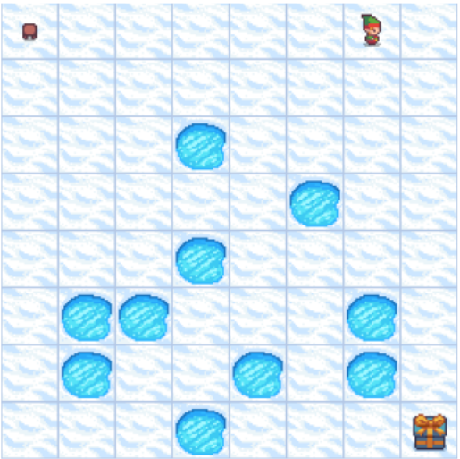
(b) Frozen Lake

Figure 1: Gymnasium environments we use for actual fitness-score evaluation.

IV-A Blackjack

Blackjack is a popular single-player card game played between a player and a dealer. The objective is to obtain a hand value closer to 21 than the dealer’s hand value—without exceeding 21 (going bust). We follow the game rules defined by Sutton and Barto [30]. Each face card counts as 10, and an ace can be counted as either 1 or 11. The https://gymnasium.farama.org/environments/toy_text/blackjack/Blackjack environment of Gymnasium represents a state based on three factors: 1) the sum of the player’s card values, 2) the value of the dealer’s face-up card, and 3) whether the player holds a usable ace. An ace is usable if it can count as 11 points without going bust. Each state allows two possible actions: stand (refrain from drawing another card) or hit (draw a card).

We represent an individual as a binary vector, where each cell corresponds to a game state from which an action can be taken; the cell value indicates the action taken when in that state. As explained by Sutton and Barto [30], there are 200 such states, therefore the size of the search space is $2^{200}$.

The actual fitness score of an individual is computed by running 100,000 games in the simulator and then calculating the difference between the number of wins and losses. We normalize fitness by dividing this difference by the total number of games. The ML models and the GA receive the normalized results (i.e., scores $\in[-1,1]$), but we will display the non-normalized fitness scores for easier readability. Given the inherent advantage of the dealer in the game, it is expected that the fitness scores will mostly be negative.

IV-B Frozen Lake

In this game, a player starts at the top-left corner of a square board and must reach the bottom-right corner. Some board tiles are holes. Falling into a hole leads to a loss, and reaching the goal leads to a win. Each tile that is not a hole is referred to as a frozen tile.

Due to the slippery characteristics exhibited by the frozen lake, the agent might move in a perpendicular direction to the intended direction. For instance, suppose the agent attempts to move right, after which the agent has an equal probability of $\frac{1}{3}$ to move either right, up, or down. This adds a stochastic element to the environment and introduces a dynamic element to the agent’s navigation.

For consistency and comparison, all simulations will run on the 8x8 map presented in fig:problems. In this map, the https://gymnasium.farama.org/environments/toy_text/frozen_lake/Frozen Lake environment represents a state as a number between $0$ and $63$. There are four possible actions in each state: move left, move right, move up, or move down. Our GA thus represents a Frozen Lake agent as an integer vector with a cell for each frozen tile on the map, except for the end-goal state (since no action can be taken from that state). Similarly to Blackjack, each cell dictates the action being taken when in that state. Since there are 53 frozen tiles excluding the end-goal, the size of the search space is $4^{53}$. The fitness function is defined as the percentage of wins out of 2000 simulated games. Again, we will list non-normalized fitness scores.

V Proposed Method

This section presents our proposed method for fitness approximation in GAs using ML models. We outline the steps involved in integrating Ridge and Lasso regressors into the GA framework, and end with a discussion of advantages and limitations of the new method.

V-A Population Dataset

Our approach combines both offline and online learning, as depicted in fig:fit-approx. The algorithm begins in evolution mode, functioning as a regular GA, where a population evolves over successive generations. However, each time a fitness score is computed for an individual, we update a dataset whose features are the encoding vector of the individual and whose target value is the respective fitness score. An illustration of the dataset is presented in tab:dataset. The initial population will always be evaluated using the simulator since the population dataset is empty at this stage of the run.

Figure 2: Flowchart of proposed method. In evolution mode the algorithm functions as a regular GA. When the switch condition is met the algorithm shifts to prediction mode: actual (in-simulator) fitness values are calculated only for a sampled subset of the population, while the rest are assigned approximate fitnesses from the ML model. This latter is retrained before moving to the next generation.

TABLE I: An example of a dataset created during a GA run of the Frozen Lake environment. An individual is a vector of 53 attributes. A total of $m$ fitness computations have been carried out so far.

Index	$\boldsymbol{a_{1}}$	$\boldsymbol{a_{2}}$	…	$\boldsymbol{a_{53}}$	Fitness
1	1	0	…	1	0.83
2	3	2	…	0	0.42
…	…	…	…	…	…
m	2	0	…	2	0.19

After a predefined switch condition is met the algorithm transitions from evolution mode to prediction mode. In prediction mode, actual (in-simulator) fitness scores are computed only for a sampled subset of the population. For the rest of the population the GA assigns approximate fitness values using a learned ML model that was trained on the existing population dataset. The algorithm can switch back and forth between evolution mode and prediction mode, enabling dynamic adaptation to the evolutionary state.

Specifically, in evolution mode, the following happens:

1. Actual (in-simulator) fitness scores of the entire population are computed.

2. The ML dataset is updated with the population’s individuals and their actual fitnesses.

3. A new ML model is fitted to the updated dataset.

In prediction mode, the following happens:

1. A subset of the population is sampled per generation.

2. Actual (in-simulator) fitness scores of the sampled individuals are computed.

3. The ML model predicts (approximate) fitness scores for the rest of the population.

4. The ML dataset is updated with the sampled individuals and their actual (in-simulator) fitness.

5. A new ML model is fitted to the updated dataset to be used by the next generation.

Witness the interplay between the dynamic switch condition and the static (pre-determined) sample rate—a hyperparameter denoting the percentage of the population being sampled. In cases where lower runtimes are preferred, using a relatively lenient switch condition is better, resulting in a higher fitness-approximation rate coupled with reduced runtime—at some cost to fitness quality. On the contrary, in cases where accurate fitness scores are preferred, the use of a strict switch condition is advisable, to allow ML fitness approximation only when model confidence is high.

Note that the number of actual, in-simulator fitness computations performed is ultimately determined dynamically by the coaction of switch condition and sample rate.

In stochastic domains such as ours, the same individual may receive different (actual) fitness scores for every evaluation, and thus appear in the population dataset multiple times—with different target values. This can be prevented by keeping a single copy of each individual in the dataset, or by computing an average fitness score of all evaluations of the same individual (or possibly some other aggregate measure). However, since these solutions greatly interfere with the sample weighting mechanism (described in sec:sample-weights), we decided to remove identical duplicate rows only (i.e., with both equal representations and fitness scores) while keeping individuals with equal representation and different fitness scores in the dataset.

V-B Switch condition

The switch condition plays a crucial role in determining when the GA transitions from evolution mode to prediction mode (and vice-versa). Our approach defines the switch condition based on a predefined criterion. Once this criterion is met, the algorithm switches its focus from evolving based entirely on full fitness computation to obtaining approximate fitness values through the model.

The switch condition can be defined in various ways depending on the specific problem and requirements. It may involve measuring the accuracy of the model’s predictions, considering a predefined threshold, or other criteria related to the state of the population and the model. In situations where the model’s accuracy falls below the desired threshold, the algorithm can revert back to evolution mode until the condition for switching to prediction mode is met once again.

Determining an appropriate switch condition is crucial for balancing the trade-off between the accuracy of fitness approximation and the computational efficiency of the algorithm. It requires tuning to find the optimal configuration for a given problem domain. Overall, the switch condition serves as a pivotal component in our approach, enabling a smooth transition from evolution mode to prediction mode based on a predefined criterion.

We defined and tested four different switch conditions, each having a hyperparameter called switch_threshold:

1. Dataset size. The simplest solution entailed performing regular evolution until the dataset reaches a certain size threshold, and then transitioning to prediction mode indefinitely. Although simple, this switch condition is less likely to adapt to the evolutionary state due to its inability to switch back to evolution mode.

2. Plateau. Wait for the best fitness score to stabilize before transitioning to prediction mode. We consider the best fitness score as stable if it has not changed much (below a given threshold) over the last $P$ generations, for a given $P$. This method posed a problem, as the model tend to maintain the evolutionary state without significant improvement throughout the run.

3. CV error. Evaluate the model’s error using cross-validation on the dataset. We switch to predict mode when the error falls below a predetermined threshold, and vice versa. We will demonstrate the use of this switch condition in the Frozen Lake scenario.

4. Cosine similarity. Cosine similarity is a metric commonly used in Natural-Language Processing to compare different vectors representing distinct words. We use this metric to compare the vectors in the GA population with those in the ML dataset. The underlying idea is that the model will yield accurate predictions if the current population closely resembles the previous populations encountered by the model, up to a predefined threshold. Our method utilizes this switch condition in the Blackjack scenario.

V-C Sampling strategy

As mentioned in sec:dataset, during prediction mode, a subset of the population is sampled in each generation. There are several sampling strategies, and choosing the right strategy can greatly impact the quality of the population dataset.

1. Random sampling. The most straightforward sampling strategy is to randomly pick a subset of the population and compute their actual fitness scores while approximating the fitness scores for the rest of the population. This strategy is useful for domains where similar individual representations do not necessarily imply similar fitness scores.

2. Similarity sampling. Another approach is choosing the individuals that are the least similar to the individuals that already exist in the dataset. Using this method will improve the diversity of the dataset and hence improve the ability of the model to generalize better to a wider volume of the search space. This strategy is useful for domains where individuals with similar representations receive similar fitness scores, such as our domains. The similarity metric we chose is the cosine similarity, discussed above.

Our generic method allows for the seamless integration of additional, more-sophisticated strategies, such as ones with a dynamic sample rate according to the evolutionary state, strategies that sample less frequently than every generation, etc.

V-D Sample weights

In this section, ‘sample’ refers to a row in the dataset (as is customary in ML)—not to be confused with ‘sampling’ in ‘sampling strategy’, introduced in the previous section.

During the training of the ML model on the dataset, each individual typically contributes equally. However, individuals tend to change and improve over the course of evolution. To account for this, we track the generation in which each individual is added to the dataset and assign weights accordingly. The weight assigned to an individual increases with the generation number. After experimenting with various weighting functions, we established a square root relationship between the generation number and its corresponding weight: $\mathit{weight}=\mathit{\sqrt{gen}}$. We note that the algorithms we used do not require the weights to sum to one.

V-E Advantages and limitations

Our proposed method offers several advantages. It can potentially reduce the computational cost associated with evaluating fitness scores in a significant manner. Rather than compute each individual’s fitness every generation, the population receives an approximation from the ML model at a negligible cost.

The use of models like Ridge and Lasso helps avoid overfitting by incorporating regularization. This improves the generalization capability of the fitness-approximation model.

Additionally, our approach allows for continuous learning, by updating the dataset and retraining the model during prediction mode. The continual retraining is possible because the ML algorithms are extremely rapid and the dataset is fairly small.

There are some limitations to consider. Linear models assume a linear relationship between the input features and the target variable. Therefore, if the fitness landscape exhibits non-linear behavior, the model may not capture it accurately. In such cases, alternative models capable of capturing non-linear relationships may be more appropriate; we plan to consider such models in the future.

Further, the performance of the fitness-approximation model heavily relies on the quality and representativeness of the training dataset. If the dataset does not cover the entire search space adequately, the model’s predictions may be less accurate. Careful consideration should be given to dataset construction and sampling strategies to mitigate this limitation.

An additional limitation is the choice of the best individual to be returned at the end of the run. Since a portion of the fitness values is approximate, the algorithm might return an individual with a good predicted fitness score, but with a bad actual fitness score. To address this issue, we first tried to keep the best individual in each generation (whether in evolution or prediction mode), compute the actual fitness values of these individuals at the end of the run, and return the best of them. Due to the approximate fitness scores being less accurate, this approach was found lacking. Instead, we found a simpler solution: Return the individual with the best fitness from the population dataset (which always holds actual fitness values). This solution did not require an actual fitness computation at the end of the run, as with the previous approach, and also improved the results by returning better fitness scores on average.

VI Experiments and Results

To assess the efficacy of the proposed approach, we carried out a comprehensive set of experiments aimed at solving the two problems outlined in sec:problems. Our objective was to compare the performance of our method against a “full” GA (computing all fitnesses), considering solution quality and computational efficiency as evaluation criteria.

Experiments were conducted using the EC-KitY software [27] on a cluster of 96 nodes and 5408 CPUs (the most powerful processors are AMD EPYC 7702P 64-core, although most have lesser specs). 10 CPUs and 3 GB RAM were allocated for each run. Since the nodes in the cluster vary in their computational power, and we had no control over the specific node allocated per run, we measured computational cost as number of actual (in-simulator) fitness computations performed, excluding the initial-population fitness computation. The average duration of a single fitness computation was 21 seconds for Blackjack and 6 seconds for Frozen Lake. The source code for our method and experiments can be found in our https://github.com/itaitzruia4/ApproxMLGitHub repository.

Both fitness-approximation runs and full-GA runs included the same genetic operators with the same probabilities: tournament selection [1], two-point crossover [29], bit-flip mutation for Blackjack and uniform mutation for Frozen Lake [19]. The specific hyperparameters utilized in the experiments and their chosen values are detailed in tab:hyperparameters.

TABLE II: Hyperparameters.

Hyperparameter	Explanation	Blackjack	Frozen Lake
switch_condition	see sec:switch	Cosine	CV Error
switch_threshold	see sec:switch	0.9	0.02
population_size	number of individuals in population	100	100
p_crossover	crossover rate between two individuals	0.7	0.7
p_mutation	mutation probability per individual	0.3	0.3
generations	number of generations	200	50
tournament_size	for tournament selection	4	4
crossover_points	number of crossover points for $K$-point crossover	2	2
mutation_points	number of mutation points for $N$-point mutation	20	6
model	type of model that predicts fitness scores	Ridge	Lasso
alpha	model regularization parameter	0.3	0.65
max_iter	maximum iterations for ML training algorithm	3000	1000
gen_weight	weighting function, discussed in sec:sample-weights	sqrt	sqrt

We performed 20 replicates per sample rate, and assessed statistical significance by running a 10,000-round permutation test, comparing the mean scores between our proposed method and the full GA (with full fitness computation). The results are shown in tab:perm-tests.

TABLE III: Results. Each row summarizes 20 replicate runs. The last row represents the full GA. Sample rate: proportion of fitness values computed in prediction mode. Absolute fitness: mean best-of-run fitness values of all replicates. Relative fitness: Absolute fitness compared to GA (percentage). Absolute computations: mean number of actual fitness computations done in simulator across all replicates. Relative computations: Absolute computations compared to GA (percentage). p-value: result of 10,000-round permutation test, comparing the mean scores between our proposed method and the full GA (with full fitness computation). Boldfaced results are those that are statistically identical in performance to full GA, i.e., p-value $>0.05$.

Sample	Absolute	Relative	Absolute	Relative	p-value
rate	fitness	fitness	computations	computations
20%	-4517.45	84.92%	4196	20.98%	1e-4
40%	-4018.9	95.46%	8075	40.38%	4.5e-3
60%	-3904.65	98.25%	12,022	60.11%	0.13
80%	-3803.55	100.86%	16,006	80.03%	0.46
GA	-3836.4	100%	20,000	100%

(a) Blackjack

Sample	Absolute	Relative	Absolute	Relative	p-value
rate	fitness	fitness	computations	computations
20%	1064.6	84.91%	2512	50.24%	1e-4
40%	1223.2	97.56%	4325	86.5%	0.11
60%	1248.9	97.16%	4730	94.6%	0.8
80%	1262.95	100.73%	4892	97.84%	0.58
GA	1253.75	100%	5000	100%

(b) Frozen Lake

Examining the results reveals an observable rise in fitness scores, along with an increase in the number of fitness computations, as sample rate increases. This is in line with the inherent trade-off within our method, wherein the quality of the results and the runtime of the algorithm are interconnected. Further, there is a strong correlation between the sample rate and the relative number of fitness computations. Notably, as the relative fitness-score computation approaches the sample rate, the frequency of individuals with approximate fitness scores increases.

In the Blackjack scenario, fitness-computation ratios closely approximate the sample rates, indicating a strong dominance of prediction mode. In contrast, computation ratios for Frozen Lake are relatively close to 100%, with the exception of the 20% sample rate, signifying a prevalence of evolution mode in the majority of generations. Note that even in this case we attained significant savings at virtually zero cost.

These observations shed light on the impact of the switch condition and its predefined threshold hyperparameters on the behavior of the algorithm in approximating fitness scores.

Boldfaced results in tab:perm-tests are those that are statistically identical in performance to the full GA, i.e., p-value $>0.05$.

We observe that results indistinguishable from the full GA can be obtained with a significant reduction in fitness computation.

tab:comparison shows the performance of three methods discussed in sec:prev: HEA/FA [10], Averaged Fitness Inheritance [28], and Proportional Fitness Inheritance [28]. We contacted the authors for the implementation of the papers (unfortunately, they are not available on GitHub) but received no reply—so we implemented the methods ourselves.

HEA/FA algorithm produced unsatisfactory results, whereas the other two performed relatively well, especially for the Frozen Lake problem. However, statistical insignificance (meaning, same as full GA) was only attained at 80% sample rate in Frozen Lake (and not at all in Blackjack)—whereas our method achieved statistical insignificance for both problems and for lower sample rates as well, as can be seen in tab:perm-tests. In summary: Compare the boldfaced lines (or lack thereof) of tab:perm-tests and tab:comparison.

TABLE IV: Previous work: Results. HEA/FA: Our implementation of the method suggested by Guo et al. [10]. Avg-FI: Our implementation of Average Fitness Inheritance, as suggested by Smith et al. [28]. Prop-FI: Our implementation of Proportional Fitness Inheritance as suggested by Smith et al. [28], using Cosine Similarity as similarity metric.

Method	Sample	Absolute	Relative	Absolute	Relative	p-value
	rate	fitness	fitness	computations	computations
HEA/FA	20%	-16525.7	23.21%	4280.45	21.4%	1e-4
HEA/FA	40%	-15042	25.5%	8318.63	41.59%	1e-4
HEA/FA	60%	-14751.3	26.01%	12,381.85	61.9%	1e-4
HEA/FA	80%	-13,831.58	27.74%	16,413.89	82.07%	1e-4
Avg-FI	20%	-8523.8	45.01%	4000	20%	1e-4
Avg-FI	40%	-7508.95	51.09%	8000	40%	1e-4
Avg-FI	60%	-5601.5	68.49%	12,000	60%	1e-4
Avg-FI	80%	-4031.05	95.17%	16,000	80%	2e-4
Prop-FI	20%	-9093.45	42.19%	4000	20%	1e-4
Prop-FI	40%	-7206.45	53.24%	8000	40%	1e-4
Prop-FI	60%	-5738.75	66.85%	12,000	60%	1e-4
Prop-FI	80%	-4023.7	95.35%	16,000	80%	9e-4
GA		-3836.4	100%	20,000	100%

(a) Blackjack

Method	Sample	Absolute	Relative	Absolute	Relative	p-value
	rate	fitness	fitness	computations	computations
HEA/FA	20%	463.1	36.94%	1129.7	22.59%	1e-4
HEA/FA	40%	434.95	34.92%	2124.15	42.48%	1e-4
HEA/FA	60%	482.5	38.48%	3125.15	62.5%	1e-4
HEA/FA	80%	523.75	41.77%	4120.45	82.41%	1e-4
Avg-FI	20%	1005.35	80.19%	1000	20%	1e-4
Avg-FI	40%	1103.8	88.04%	2000	40%	1e-4
Avg-FI	60%	1187.65	94.73%	3000	60%	4.7e-3
Avg-FI	80%	1238.55	98.79%	4000	80%	0.39
Prop-FI	20%	938.3	74.84%	1000	20%	1e-4
Prop-FI	40%	1077.2	85.92%	2000	40%	1e-4
Prop-FI	60%	1171.7	93.46%	3000	60%	1e-3
Prop-FI	80%	1218.4	97.18%	4000	80%	0.07
GA		1253.75	100%	5000	100%

(b) Frozen Lake

VII Extensions

VII-A Novelty search

As mentioned in sec:advantages-limitations, the model should cover a large volume of the search space in order to generalize well to new individuals created by the genetic operators throughout the evolutionary run. We tested an alternative method to initialize the initial population (line 1 in alg:ga). Instead of randomly generating the initial population, we perform Novelty Search [18].

In novelty search, fitness is abandoned in favor of finding distinct genomes, the idea being to keep vectors that are most distant than their $n$ nearest neighbors in the population (we used $n=20$). This causes the individuals to be relatively far from each other at the end of novelty search, and thus cover a larger volume of the search space.

After this new initialization procedure the algorithm behaves exactly as in sec:method.

The results, shown in tab:novelty, indicate a minimal difference in fitness scores (cf. tab:perm-tests) when using this approach. However, this initialization may be useful in other domains, possibly with larger search spaces.

TABLE V: Initialization through novelty search: Results.

Sample	Absolute	Relative	Absolute	Relative	p-value
rate	fitness	fitness	computations	computations
20%	-4495.55	85.38%	4192	20.96%	1e-4
40%	-4009.95	95.67%	8066	40.33%	9e-4
60%	-3877.7	98.93%	12,026	60.13%	0.35
80%	-3848.75	99.67%	16,013	80.07%	0.81
GA	-3836.4	100%	20,000	100%

(a) Blackjack

Sample	Absolute	Relative	Absolute	Relative	p-value
rate	fitness	fitness	computations	computations
20%	1159	92.44%	2836	56.72%	3e-4
40%	1254.65	100%	4295	85.9%	0.97
60%	1241.95	99.06%	4700	94%	0.6
80%	1231.4	98.21%	4882	97.64%	0.26
GA	1253.75	100%	5000	100%

(b) Frozen Lake

VII-B Hidden actual fitness scores in prediction mode

In most existing fitness-approximation methods, as discussed in sec:prev, some individuals in the population have their fitness values approximated, while the rest receive actual fitness scores. Our preliminary investigation, which employed this scheme, suggested that individuals with actual fitness scores might “hijack” the evolutionary process. In cases of pessimistic approximations the individuals with actual fitness scores are likely to be selected, to then repeatedly reproduce, thus restricting the exploration of the search space.

In evolution mode of our baseline method, the actual fitness scores are both given to the GA and added to the ML dataset. Another approach is to hide actual fitness scores from the GA in prediction mode, only adding them to the ML dataset. The sampled individuals still receive approximate fitness scores, even though their actual fitness scores are computed. Such an approach is implemented in the proposed solution of Guo et al. [10].

This latter approach harms the accuracy of the fitness scores, since the approximate fitness scores are usually less accurate than the actual fitness scores. On the other hand, this approach prevents the potential problem described above. In contrast to the baseline method, the calculation of the actual fitness scores and model training in prediction mode is independent of the evolutionary process when fitness scores are hidden from the GA. As a result, fitness computation and model training can be executed as separate processes in parallel, significantly decreasing runtime. By our calculations this parallelization could result in a speedup of up to 60% in the runtime of our existing method. We plan to perform concrete experiments on this approach in the future.

VIII Concluding Remarks and Future Work

In this paper we presented a generic method to integrate machine learning models in fitness approximation. Our approach is useful for domains wherein the fitness score calculation is computationally expensive, such as running a simulator. We used Gymnasium simulators for evaluating actual fitness scores, and Ridge and Lasso models for learning the fitness-approximation models.

Our analysis includes a rigorous comparison between different methods for: 1) switching between actual and approximate fitness, 2) sampling the population, and 3) weighting the samples.

Our results show a significant reduction in GA runtime, with a small price in fitness for low sample rates, and no price for high sample rates.

Further enhancements can be incorporated into our method by employing more complex ML models, such as Random Forest [2], XGBoost [5], or Deep Networks [25]. While these models have the potential to improve fitness approximation, it is worth noting that they are typically computationally intensive and may not be suitable for domains with limited fitness computation time.

Additionally, our method can be refined by leveraging domain-specific knowledge or advanced data science concepts, to improve the generality of the population dataset and, consequently, the accuracy of the model. These approaches have the potential to enhance the overall performance of our solution.

References

- Blickle [2000] T. Blickle. Tournament selection. Evolutionary Computation, 1:181–186, 2000.
- Breiman [2001] L. Breiman. Random forests. Machine Learning, 45:5–32, 2001.
- Brockman et al. [2016] G. Brockman, V. Cheung, L. Pettersson, J. Schneider, J. Schulman, J. Tang, and W. Zaremba. OpenAI gym. arXiv preprint arXiv:1606.01540, 2016.
- Chen et al. [2002] J.-H. Chen, D. E. Goldberg, S.-Y. Ho, and K. Sastry. Fitness inheritance in multi-objective optimization. In GECCO 2002, volume 2, pages 319–326, 2002.
- Chen and Guestrin [2016] T. Chen and C. Guestrin. XGBoost: A scalable tree boosting system. In Proceedings of the 22nd ACM SIGKDD International Conference on Knowledge Discovery and Data Mining, pages 785–794, 2016.
- Dias et al. [2014] J. Dias, H. Rocha, B. Ferreira, and M. d. C. Lopes. A genetic algorithm with neural network fitness function evaluation for IMRT beam angle optimization. Central European Journal of Operations Research, 22(3):431–455, 2014.
- Drucker et al. [1996] H. Drucker, C. J. Burges, L. Kaufman, A. Smola, and V. Vapnik. Support vector regression machines. Advances in Neural Information Processing Systems, 9, 1996.
- Elyasaf et al. [2012] A. Elyasaf, A. Hauptman, and M. Sipper. Evolutionary Design of Freecell Solvers. IEEE Transactions on Computational Intelligence and AI in Games, 4(4):270–281, 2012.
- García-Sánchez et al. [2020] P. García-Sánchez, A. Tonda, A. J. Fernández-Leiva, and C. Cotta. Optimizing hearthstone agents using an evolutionary algorithm. Knowledge-Based Systems, 188:105032, 2020.
- Guo et al. [2017] P. Guo, W. Cheng, and Y. Wang. Hybrid evolutionary algorithm with extreme machine learning fitness function evaluation for two-stage capacitated facility location problems. Expert Systems with Applications, 71:57–68, 2017.
- Hemanth and Anitha [2019] D. J. Hemanth and J. Anitha. Modified genetic algorithm approaches for classification of abnormal magnetic resonance brain tumour images. Applied Soft Computing, 75:21–28, 2019.
- Hoerl and Kennard [1970] A. E. Hoerl and R. W. Kennard. Ridge regression: Biased estimation for nonorthogonal problems. Technometrics, 12(1):55–67, 1970.
- Holland [1992] J. H. Holland. Genetic algorithms. Scientific American, 267(1):66–73, 1992.
- James et al. [2023] G. James, D. Witten, T. Hastie, R. Tibshirani, and J. Taylor. An Introduction to Statistical Learning with Applications in Python. Springer Texts in Statistics. Springer Cham, 2023.
- Jha and Eyong [2018] S. K. Jha and E. M. Eyong. An energy optimization in wireless sensor networks by using genetic algorithm. Telecommunication Systems, 67:113–121, 2018.
- Jin [2005] Y. Jin. A comprehensive survey of fitness approximation in evolutionary computation. Soft Computing, 9(1):3–12, 2005.
- Koza [1992] J. R. Koza. Genetic Programming: On the Programming of Computers by Means of Natural Selection. MIT press, 1992.
- Lehman and Stanley [2011] J. Lehman and K. O. Stanley. Abandoning objectives: Evolution through the search for novelty alone. Evolutionary Computation, 19(2):189–223, 2011.
- Lim et al. [2017] S. M. Lim, A. B. M. Sultan, M. N. Sulaiman, A. Mustapha, and K. Y. Leong. Crossover and mutation operators of genetic algorithms. International Journal of Machine Learning and Computing, 7(1):9–12, 2017.
- Livne et al. [2022] A. Livne, E. S. Tov, A. Solomon, A. Elyasaf, B. Shapira, and L. Rokach. Evolving context-aware recommender systems with users in mind. Expert Systems with Applications, 189:116042, 2022.
- Mayer et al. [2020] M. J. Mayer, A. Szilágyi, and G. Gróf. Environmental and economic multi-objective optimization of a household level hybrid renewable energy system by genetic algorithm. Applied Energy, 269:115058, 2020.
- Miller [2011] J. F. Miller. Cartesian genetic programming. In Cartesian Genetic Programming, pages 17–34. Springer, 2011.
- O’Neill and Ryan [2001] M. O’Neill and C. Ryan. Grammatical evolution. IEEE Transactions on Evolutionary Computation, 5(4):349–358, 2001.
- Pedregosa et al. [2011] F. Pedregosa, G. Varoquaux, A. Gramfort, V. Michel, B. Thirion, O. Grisel, M. Blondel, P. Prettenhofer, R. Weiss, V. Dubourg, et al. Scikit-learn: Machine learning in python. Journal of Machine Learning Research, 12:2825–2830, 2011.
- Prince [2023] S. J. Prince. Understanding Deep Learning. MIT Press, 2023. URL https://udlbook.github.io/udlbook/.
- Schmidt and Lipson [2008] M. D. Schmidt and H. Lipson. Coevolution of fitness predictors. IEEE Transactions on Evolutionary Computation, 12(6):736–749, 2008.
- Sipper et al. [2023] M. Sipper, T. Halperin, I. Tzruia, and A. Elyasaf. EC-KitY: Evolutionary computation tool kit in Python with seamless machine learning integration. SoftwareX, 22:101381, 2023.
- Smith et al. [1995] R. E. Smith, B. A. Dike, and S. Stegmann. Fitness inheritance in genetic algorithms. In Proceedings of the 1995 ACM Symposium on Applied Computing, pages 345–350, 1995.
- Spears and Anand [1991] W. M. Spears and V. Anand. A study of crossover operators in genetic programming. In International Symposium on Methodologies for Intelligent Systems, pages 409–418. Springer, 1991.
- Sutton and Barto [2018] R. S. Sutton and A. G. Barto. Reinforcement Learning: An Introduction. MIT press, 2018.
- Tibshirani [1996] R. Tibshirani. Regression shrinkage and selection via the lasso. Journal of the Royal Statistical Society Series B: Statistical Methodology, 58(1):267–288, 1996.
- Yu and Kim [2018] D.-P. Yu and Y.-H. Kim. Is it worth to approximate fitness by machine learning? investigation on the extensibility according to problem size. In 2018 Proceedings of the Genetic and Evolutionary Computation Conference Companion, pages 77–78, 2018.
- Zhang et al. [2022] Y. Zhang, M. C. Fontaine, A. K. Hoover, and S. Nikolaidis. Deep surrogate assisted map-elites for automated hearthstone deckbuilding. In Proceedings of the Genetic and Evolutionary Computation Conference, pages 158–167, 2022.