Spatial data fusion adjusting for preferential sampling using INLA and SPDE

Abstract

Spatially misaligned data can be fused by using a Bayesian melding model that assumes that underlying all observations there is a spatially continuous Gaussian random field process. This model can be used, for example, to predict air pollution levels by combining point data from monitoring stations and areal data from satellite imagery. However, if the data presents preferential sampling, that is, if the observed point locations are not independent of the underlying spatial process, the inference obtained from models that ignore such a dependence structure might not be valid. In this paper, we present a Bayesian spatial model for the fusion of point and areal data that takes into account preferential sampling. The model combines the Bayesian melding specification and a model for the stochastically dependent sampling and underlying spatial processes. Fast Bayesian inference is performed using the integrated nested Laplace approximation (INLA) and the stochastic partial differential equation (SPDE) approaches. The performance of the model is assessed using simulated data in a range of scenarios and sampling strategies that can appear in real settings. The model is also applied to predict air pollution in the USA.

[1]organization=Computer, Electrical and Mathematical Science and Engineering Division, King Abdullah University of Science and Technology (KAUST),city=Thuwal, postcode=23955-6900, state=Makkah, country=Saudi Arabia

1 Introduction

Spatially misaligned data arise in a wide range of disciplines. For example, air pollution levels, defined in practice in a continuous surface, may be only available as point-level data obtained from monitoring stations placed at specific locations, and areal-level data can be measured as aggregated values at cells of a raster grid. Spatial models that aim to integrate spatial data available at varying spatial resolutions are preferred over methods that just use one type of data—as they enable optimal utilization of all available information and enhance inferential outcomes. Bayesian hierarchical models offer a viable solution for the combination of multiple spatially misaligned data. For example, Fuentes and Raftery (2005) introduced a Bayesian melding model that assumes the presence of a latent spatial process underlying all types of observations, enabling predictions by fusing all data types. Berrocal et al. (2010), on the other hand, devised a linear regression model with spatially varying coefficients, employing point data as the response variable and areal data as covariates. Moraga et al. (2017) presented an implementation of Bayesian melding model for data fusion using the integrated nested Laplace approximation (INLA) (Rue et al., 2009) and a modification of the stochastic partial differential approach (SPDE) approach (Lindgren et al., 2011), providing a computationally effective alternative to existing Markov chain Monte Carlo (MCMC) methods.

When point data is considered, preferential sampling may occur when the spatial process and sampling locations exhibit stochastic dependence (Diggle et al., 2010; Cecconi et al., 2016). This phenomenon has significant implications for spatial modeling, affecting both prediction accuracy and statistical inference (Diggle et al., 2010; Conn et al., 2017; Cappello and Palacios, 2022). In geostatistical modeling, Diggle et al. (2010) consider preferential sampling information in the model by using a shared latent process model, which is estimated using Monte Carlo methods. In this regard, Dinsdale et al. (2019) developed improved numerical approximation methods for the likelihood function, resulting in more accurate estimation than original Monte Carlo approaches. In a Bayesian framework, Pati et al. (2011) developed an approach to preferential sampling and studied its theoretical properties under an improper prior. Also, Krainski et al. (2018) implemented the Diggle et al. (2010) model within a Bayesian hierarchical framework using the INLA-SPDE approach, which offers computational efficiency and enables the prediction at fine spatial surfaces. Most recently, Shirota and Gelfand (2022) extended the preferential sampling on a bivariate geostatistical model, including a point-point misaligned setting.

In this paper, we propose a Bayesian hierarchical model to combine data available at several spatial scales adjusting for preferential sampling. This model can be used in situations as the one represented in Figure 1. In that figure, the true latent spatial field is represented together with the sampling sites. The figure shows that these sites are concentrated in areas where the represented surface assumes high values, as we are under a preferential sampling setting. This figure also shows areal data that arise from the true field aggregated into small areas. In situations like this, methods for combining point- and areal-level data might also need to adjust for preferential sampling to obtain valid inferences.

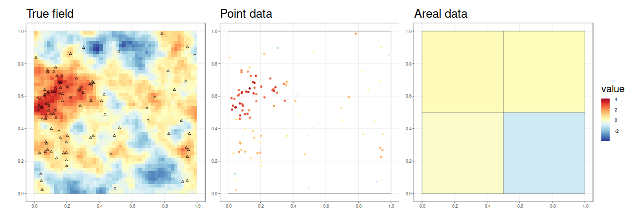
Figure 1: Example of spatially misaligned data with point data observed under preferential sampling. Left: continuous surface and sampled locations. Middle: point data with surface values at the sampled points. Right: Areal data with aggregated values of the continuous surface at areas.

Motivated by Fuentes and Raftery (2005) and Moraga et al. (2017), we specify a Bayesian hierarchical model to integrate data at different spatial resolutions by assuming a common spatial random field underlying all observations. We also account for preferential sampling by assuming a shared latent spatial random field for the intensity of the inhomogeneous Poisson point process that originates the point locations with a parameter controlling the degree of preferential sampling as described by Diggle et al. (2010). Additionally, we describe how to efficiently fit the model by using the INLA and SPDE approaches (Rue et al., 2009; Lindgren et al., 2011). To the best of our knowledge, this study represents the first attempt for spatial data fusion taking into account preferential sampling.

The remainder of this paper is structured as follows. In Section 2, we present the new model to combine spatially misaligned data under preferential sampling. Section 3 gives details of the implementation of the method using the INLA and SPDE approaches. Next, we conduct a simulation study to assess the performance of the proposed model in comparison with two alternative models that do not combine data or not take into account preferential sampling. In Section 5, the proposed model is used to predict air pollution data in the United States. Lastly, our findings and future work are discussed.

2 Spatial data fusion under preferential sampling

2.1 Integration of spatially misaligned data

Spatial misalignment occurs when measurements of the variable of interest are available at different spatial resolutions. In these situations, a modeling approach that combines all types of data may yield better inferences. Fuentes and Raftery (2005) proposed a Bayesian melding model to integrate point- and areal- level data by assuming a common spatial random field, say $\phi(\cdot)$, underlying all observations. Specifically, if $Y(\boldsymbol{s_{i}})$ represent data observed at locations $\boldsymbol{s_{i}}$, and $Y(B_{j})$ the data observed in areas $B_{j}$, the model combines both types of data using the following model:

$$\begin{split}&Y(\boldsymbol{s_{i}})=\mu(\boldsymbol{s_{i}})+\phi(\boldsymbol{s_{i}})+\epsilon(\boldsymbol{s_{i}}),\\ &Y(B_{j})=\frac{1}{B_{j}}\int_{\boldsymbol{s}\in B_{j}}\left(\mu(\boldsymbol{s})+\phi(\boldsymbol{s})\right)d\boldsymbol{s}+\epsilon(B_{j}),\end{split}$$ (1)

where $\mu(\cdot)$ is the large-scale component of the model that can be explained using covariates, and $\epsilon(\cdot)$ is the independent noise of the observations.

2.2 Model-based geostatistics under preferential sampling

This model, however, does not take into account the potential preferential sampling that could occur if the sampling locations of the point observations are concentrated in regions where the values of the phenomenon under study are thought to be larger (or smaller) than average. To deal with this situation, Diggle et al. (2010) proposed a model that included a latent process $\phi(\cdot)$ shared both by the sampling locations and the measured values. In this model, the sampling locations of the point observations are modeled using a log-Gaussian Cox process (LGCP) (Cox, 1955; Møller et al., 1998). Specifically, the sampling locations follow a Poisson process with a varying intensity which is itself a stochastic process of the form

$$\log(\lambda(\boldsymbol{\boldsymbol{s}}))=\alpha(\boldsymbol{s})+\gamma\phi(\boldsymbol{\boldsymbol{s}}),$$

where $\alpha(\boldsymbol{s})$ is the large-scale component that could include covariates, and $\phi(\boldsymbol{s})$ is a zero-mean Gaussian random field (GRF). Then, conditional on $\phi(\cdot)$, the observations are modeled as

$$Y(\boldsymbol{s})=\mu(\boldsymbol{s})+\phi(\boldsymbol{\boldsymbol{s}})+\epsilon(\boldsymbol{s}),$$ (2)

where $\mu(\boldsymbol{s})$ is the large-scale component, and $\epsilon(\bm{s})$ is independent Gaussian noise.

Thus, the model accounts for preferentiality by including an unobserved, spatially continuous process $\phi(\cdot)$ that is shared both by the point process and the measured values, and the parameter $\gamma$ controls the degree of preferentiality.

2.3 Integration of spatially misaligned data under preferential sampling

Here, we propose a Bayesian hierarchical model to integrate spatially misaligned data adjusting by preferential sampling by combining the Bayesian melding model, and the shared model for preferential sampling. Let $S$ denote the sampling point process, and $\phi(\cdot)$ the shared zero-mean random effect across the set of observations $Y$. The model, which we call PSmelding in the following sections, is specified as follows:

$$\begin{split}&Y(\boldsymbol{s_{i}})\ |\ \mu(\cdot),\phi(\cdot),\tau_{s}^{2}\sim N(\mu(\boldsymbol{s_{i}})+\phi(\boldsymbol{s_{i}}),\tau_{s}^{2}),\\ &Y(B_{j})\ |\ \mu(\cdot),\phi(\cdot),\tau_{B}^{2}\sim N\left(\int_{\boldsymbol{s}\in B_{j}}(\mu(\boldsymbol{s})+\phi(\boldsymbol{s}))d\boldsymbol{s},\tau_{B}^{2}\right),\\ &S|\alpha(\cdot),\phi(\cdot),\gamma\sim\text{Poisson}(\exp(\alpha(\boldsymbol{s})+\gamma\phi(\boldsymbol{s}))),\\ &\phi\ |\ \omega_{\phi}\sim N(0,Q(\omega_{\phi})^{-1}),\\ &\gamma\sim N(0,\tau_{\gamma}^{2}).\end{split}$$ (3)

Here, $\mu(\cdot)$ and $\alpha(\cdot)$ are fixed effects for the observation and point process models. $\tau_{s}^{2}$ and $\tau_{B}^{2}$ are the precision parameters for the point and areal observations, respectively. The parameter $\gamma$ denotes the preferential degree, with a Normal distributed prior.

In our study, we assume the Gaussian random fields are isotropic and stationary, with Matérn covariance function. The Matérn covariance function is defined as

$$C(||h||)=\frac{\sigma^{2}}{2^{\nu-1}\Gamma(\nu)}\left(\kappa\left\lVert h\right\rVert\right)^{\nu}K_{\nu}\left(\kappa\left\lVert h\right\rVert\right),$$ (4)

where $||h||$ denotes the distance between locations, $\sigma^{2}$ is the variance when $||h||=0$, and $\nu$ is the smoothing parameter. The scale parameter $\kappa$ controls the spatial dependence. The Matérn covariance function can also be expressed as a function of the spatial range $\rho=\sqrt{8\nu}/\kappa$ which corresponds to the distance at with the correlation is near 0.1 (Lindgren et al., 2011).

As shown in Zhang (2004), the parameters of a Gaussian process with isotropic Matérn covariance function at dimension lower than four are not all fixed-domain asymptotic. Instead, in fixed-domains, only the microergodic parameter $\theta=\sigma^{2}\kappa^{2\nu}$, or continuous functions of it, can be consistently estimated. Therefore, in the following sections, we will consider the microergodic parameter $\theta$ to assess the performance of the proposed model.

3 Bayesian inference with the INLA and SPDE approaches

3.1 INLA

The integrated nested Laplace approximation (INLA) proposed by Rue et al. (2009) uses analytical approximations and numerical integration algorithms for Bayesian inference in latent Gaussian latent models. INLA accelerates statistical inference and estimation of the marginal distributions of parameters, and has become an alternative to Markov Chain Monte Carlo (MCMC) for latent Gaussian models (Rue et al., 2009, 2017). INLA offers a broad applicability for modeling spatial and spatio-temporal phenomena, with a specific model structure defined as

$$\begin{split}&y_{i}|{\phi},{\theta}\sim\pi(y_{i}|x_{i},{\theta}),\ i=1,\ldots,I,\\ &{\phi}|{\theta}\sim N({\mu(\theta)},{Q(\theta)}^{-1}),\\ &{\theta}\sim\pi({\theta}),\end{split}$$ (5)

where $i=1,\ldots,I$, and the observed data ${y}=(y_{1},\ldots,y_{I})$ are assumed to belong to an exponential family with mean $\mu_{i}=g^{-1}(\eta_{i})$, such that $\eta_{i}$ is the linear predictor that may include the effects of various covariates and random effects. For example, it may consist of an intercept $\alpha$, coefficients ${\beta_{k}}$ of covariates ${z_{ki}}$, and random effects ${f^{(j)}(\cdot)}$ defined in terms of covariates ${u_{ji}}$.

The latent Gaussian field $\phi$ with mean ${\mu(\theta)}$ and precision matrix ${Q(\theta)}$ is conditioned on hyperparameters ${\theta}$, which follow a prior distribution $\pi({\theta})$. The INLA methodology, with the aid of SPDE (Lindgren et al., 2011), can be used to analyze geostatistical observations assumed to originate from a Gaussian random field with Matérn covariance function as presented in the following section.

3.2 SPDE

INLA also offers support for fitting spatial models that include Gaussian random fields with Matérn covariance. Whittle (1963) illustrated that a Gaussian field with Matérn covariance function can be written as the solution of the following stochastic partial differential equations (SPDE):

$$(\kappa^{2}-\Delta)^{\alpha/2}(\tau\phi(\boldsymbol{s}))=\mathcal{W}(\boldsymbol{s}),$$ (6)

where $\Delta=\sum_{i=1}^{2}\frac{\partial^{2}}{\partial x^{2}_{i}}$ is the Laplacian, ${\phi}$ is a Gaussian random field, and $\mathcal{W}(\boldsymbol{s})$ is a Gaussian spatial white noise process. $\kappa>0$ represents the scale, $\tau$ controls the variance, and $\alpha$ is the smoothness of the Gaussian random field. Lindgren et al. (2011) derived, using a finite element method (FEM), a compacted representation with Markov properties for the solution of Equation (6), where ${\phi}$ is approximated by a weighted basis-function expansion, and the joint distribution for the weights is a Gaussian Markov random field (GMRF). INLA-SPDE uses a triangulation of the domain and piecewise linear basis functions in two dimensions. The representation of the expansion is as follows

$$\phi(\boldsymbol{s})=\sum_{k=1}^{m}\phi_{k}(\boldsymbol{s})x_{k},$$ (7)

where $m$ is the number of vertices of the triangulation, $\phi_{k}(\cdot)$ represents compactly-supported piecewise linear functions defined on each triangle equal to 1 at vertex $k$, and equal to 0 at the other vertices, and $\{x_{k}\}$ are zero-mean Gaussian distributed weights. The precision matrix of the weights is sparse due to Markov properties.

3.3 Log-Gaussian Cox process fitting using INLA and SPDE

In our proposed Bayesian melding model with preferential sampling, we assume that the locations of the point observations have been generated from a LGCP. This process has a varying intensity that depends on an Gaussian random field $\phi(\cdot)$. Illian et al. (2012) developed a fast and flexible framework for fitting LGCP using INLA that approximates the true LGCP likelihood on a regular lattice over the observation window. Later, Simpson et al. (2016) extended the numerical inference for LGCP processes to the non-lattice, unbinned data case, leading to greater flexibility and computational efficiency. The log-likelihood of a LGCP is defined as

$$\log\pi(y\mid{\phi})=|\Omega|-\int_{\Omega}\exp(\phi(\boldsymbol{s}))d\boldsymbol{s}+\sum_{i=1}^{n}\phi(\boldsymbol{s_{i}}).$$ (8)

While the SPDE model can compute the sum term exactly, the stochastic integral $\int_{\Omega}\exp({{\phi}(\boldsymbol{s})})d\boldsymbol{s}$ must be approximated by a sum. Simpson et al. (2016) approximated the integral in Equation (8) by the deterministic integration rule of the form $\int_{\Omega}f(s)ds\approx\sum_{i=1}^{p}\tilde{\alpha}_{i}f(\tilde{s}_{i})$ in the following manner:

$$\begin{split}\log\{\pi(y\mid{\phi})\}&\approx C-\sum_{i=1}^{p}\tilde{\alpha}_{i}\exp\{\sum_{k=1}^{m}x_{j}\phi_{j}(\tilde{s}_{i})\}+\sum_{i=1}^{n}\sum_{k=1}^{m}x_{j}\phi_{j}(s_{i})\\ &=C-\tilde{\alpha}^{T}\exp(A_{1}\boldsymbol{\phi})+1^{T}A_{2},\end{split}$$ (9)

where $C$ is a constant, $[A_{1}]_{ij}=\phi_{j}(\tilde{s}_{i})$ is a projection matrix containing the values of the latent Gaussian model at the integration nodes ${\tilde{s}_{i}}$, and $[A_{2}]_{ij}=\phi_{j}(s_{i})$ evaluates the latent Gaussian field at the observed points ${s_{i}}$.

Using Baddeley and Turner (2000)’s numerical integration schemes, Simpson et al. (2016) construct pseudo-observations, $y=(0_{p\times 1}^{T},1_{N\times 1}^{T})^{T}$, and approximate the likelihood using the form $\pi(y\mid{\phi})\approx C\prod_{i=1}^{n+p}\eta_{i}^{y_{i}}e^{-\alpha_{i}u_{i}}$, where $\alpha_{i}$ and $u_{i}$ correspond to the intensity function and the basis function evaluated at the $i$-th point, respectively. This likelihood approximation is similar to that of observing $N+p$ conditionally independent Poisson random variables with means $\alpha_{i}u_{i}$ and observed values $y_{i}$. Aiming at fully specifying the model, it is necessary to define an integration scheme that can be employed in Equation (9). One of the simplest approaches is to assign a region $V_{i}$ to each node within the mesh, where the basis function $\phi_{i}(s)$ takes on a greater value than any other basis function as in Figure 2. The associated integration rule involves setting $\tilde{s}_{i}$ as the location of the node, and $\tilde{\alpha}_{i}=|V_{i}|$ as the volume of the dual cell.

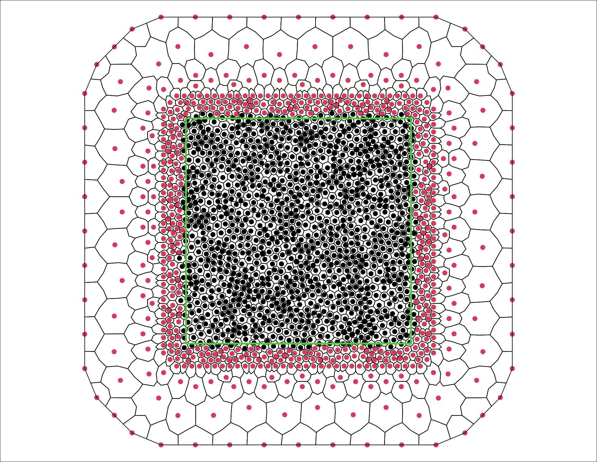
Figure 2: Dual mesh constructed by joining the centroids of the primal mesh. Black nodes represent the centroids and red nodes the integration points with zero weight. The green square is the area of interest.

Our work uses such an algorithm for estimating the models considering preferential sampling.

3.4 Spatially misaligned data modeling using INLA and SPDE

As shown in Moraga et al. (2017), spatial data available at different resolutions can be combined by using a Bayesian melding model that can be fitted using the INLA-SPDE framework. In this approach, point data, $Y(\boldsymbol{s_{i}})$, are realizations of the shared latent Gaussian random field at sites $\boldsymbol{s_{i}}$, and areal data, $Y(B_{j})$, can be represented as stochastic integrals within the areas. To reduce the computational cost, Moraga et al. (2017) used the fact that the weighted sum of the vertices in the triangulated mesh is the approximation of the integral in the area. Thus, if $A$ represents the projection matrix that maps the Gaussian Markov random field from the observations to the triangulation nodes, the areal observations can be expressed as

$$E(Y(B_{j}))=\int_{\boldsymbol{s}\in B_{j}}\phi(\boldsymbol{s})d\boldsymbol{s}\approx\sum_{k=1}^{m}x_{k}\phi_{k}(\tilde{\boldsymbol{s}}_{i})=A\phi.$$ (10)

Figure 3 illustrates the triangulation vertices used to compute the projection matrix when combining point and areal observations. For a given area $B_{j}$, the corresponding $j$-th row of the projection matrix has elements that satisfy $\sum_{i=1}^{m}[A]_{ij}=1$. For vertices outside the area, $[A]_{ij}=0$. For vertices inside the area, $[A]_{ij}=1/m_{B_{j}}$, where $m_{B_{j}}$ is the number of points contained in the area $B_{j}$, at the columns that represent the vertices of the triangles contained in the area. Note that while Moraga et al. (2017) uses equal weights for areal observations, it is also possible to use different values in situations where other factors such as population density need to be taken into account.

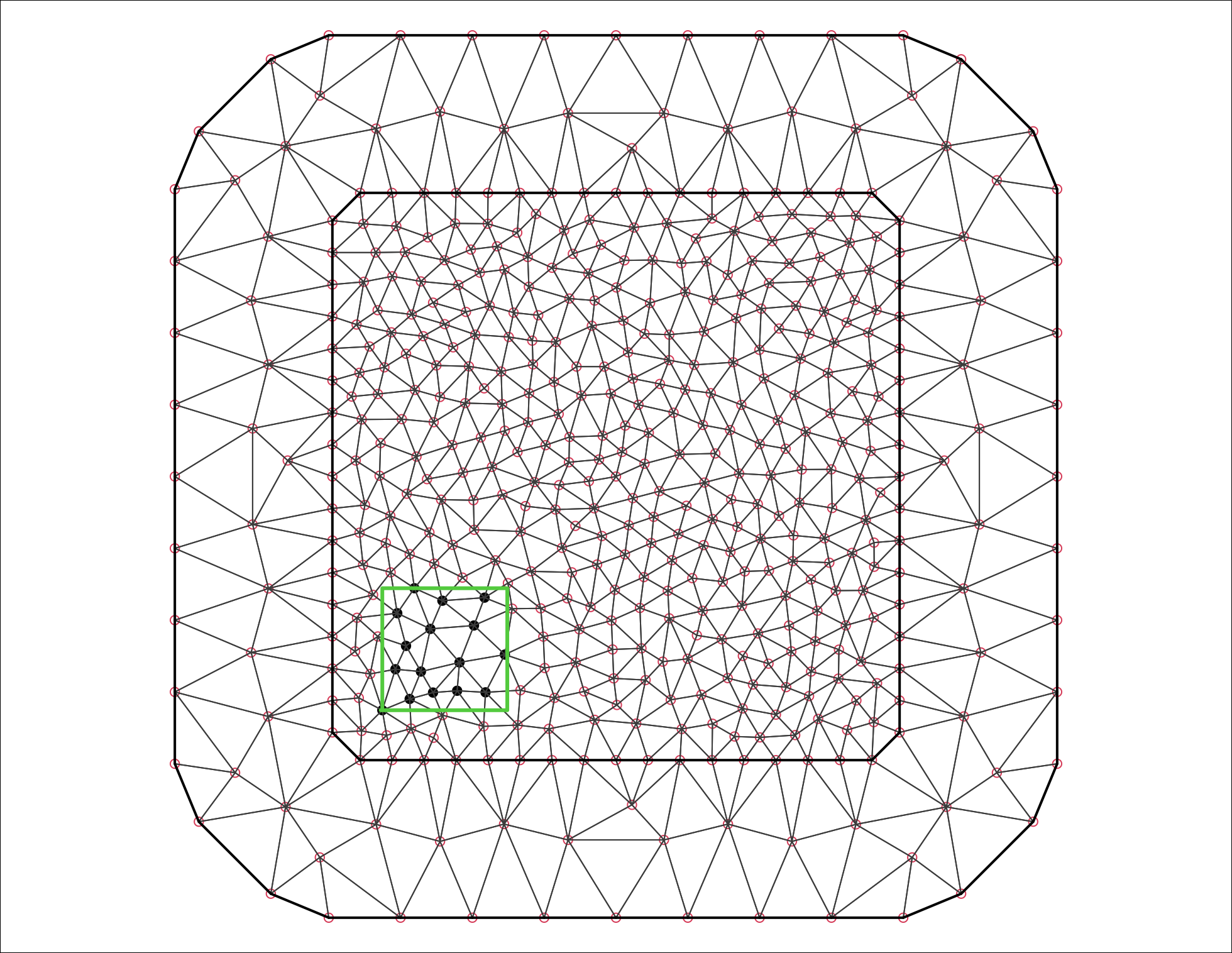
Figure 3: Triangulated mesh used in the INLA-SPDE approach. The green square represents one of the areal observations. In the row of the projection matrix corresponding to this area, the $n$ black vertices within the area are weighted $1/n$. The vertices outside the area are given zero weight.

4 Simulation study

We conduct a simulation study to show the performance of our proposed melding approach adjusting for preferential sampling (PSmelding) in comparison with the melding approach without preferential sampling adjustment (Melding) and a geostatistical model that only uses point data adjusting for preferential sampling (PSgeo).

Specifically, we assess the bias that is produced from ignoring preferential sampling when using a melding approach to combine spatially misaligned data, and how spatial data fusion model reduces the risk of misspecification when preferential sampling does not exist.

4.1 Data simulation

In all simulation scenarios, we assume the region of interest is a unit square. We generate random surfaces using several specifications for the parameters of Model (3). We then obtain point observations of the simulated surfaces at 100 and 250 randomly generated locations. We also obtain areal observations as averages of the true surfaces at cells of regular grids consisting of 4, 25 and 100 cells. Then, we fit the Melding, PSmelding and PSgeo models to different configurations of the observed data, and obtain predictions at locations of a 50 $\times$ 50 regular grid. We assess the performance of each of the models by comparing the true and simulated surfaces using several criteria. For each of the scenarios, we generate 100 spatial surfaces to have stable results.

We simulate data according to six scenarios using Model (3). In particular, we set $\mu(\bm{s})=0$. In the intensity function of the LGCP, we set $\alpha(\bm{s})=0.05$. The variance of the random noise (nugget effect) of the point and areal observations is set to 0.1, indicating precision $\tau_{s}$ = $\tau_{B}=10$. The shared spatial random effect $\phi(\cdot)$ is assumed to be a zero-mean Gaussian random field with isotropic Matérn covariance function parametrized as in Equation (4). For all scenarios, we set the parameters of the covariance function $\nu$ = 1 and $\sigma$ = 1. We set $\kappa$ equal to $\sqrt{2\nu}/s$, with $s=0.05,0.1,0.2$. This implies values of the microergodic parameter equal to $\theta=\sigma^{2}\kappa^{2\nu}=2\sigma^{2}/s^{2}$ equal to 800, 200 and 50, as seen in Table 1. A more interpretative parameter is the spatial range which is equal to $\rho=\sqrt{8\nu}/\kappa=\sqrt{8\nu}\times s/\sqrt{2\nu}=2\times s$, which corresponds to the distance at with the correlation is near 0.1. Finally, the preferential sampling degree parameter $\gamma$ is set to 0 to simulate non-preferential sampling scenarios, or to 1 to represent preferential sampling scenarios.

Table 1: Parameter values used in each of the simulation scenarios. There are six scenarios arising as combinations of microergodic parameter ($\theta$) and preferential degree ($\gamma$).

Scenario	1	2	3	4	5	6
$\rho$	0.1	0.2	0.4	0.1	0.2	0.4
$\theta$	800	200	50	800	200	50
$\gamma$	0	0	0	1	1	1

4.2 Model assessment

Aiming at assessing the results, we report the mean squared error (MSE), the mean absolute error (MAE) and the Wasserstein distance (WD) (Kantorovich, 1960) obtained for each of the simulated scenarios. The MSE is calculated by averaging the squared differences between the predictive posterior mean and the true spatial surface, whereas the MAE averages the absolute value of the differences between the predictive posterior median and the true surface. Since both MSE and MAE ignore the variability of the predictive posterior distribution, we also use the WD as a criterion to account for the whole predictive posterior distribution.

The WD has been used to assess the robustness and statistical properties of distributions arising in different fields including image analysis, metereology and astrophysics (Engquist and Froese, 2013; Zhao and Guan, 2018; Mohajerin Esfahani and Kuhn, 2018; Sun et al., 2022). Givens and Shortt (1984) provide the closed form of WD to compare Normal distributions. Specifically, if $\pi_{1}={\mathcal{N}}(\mu_{1},C_{1})$ and $\pi_{2}={\mathcal{N}}(\mu_{2},C_{2})$ are two non-degenerate Gaussian measures on $\mathbb{R}^{n}$ with respective expected values $\mu_{1},\mu_{2}\in\mathbb{R}^{n}$ and covariances $C_{1},C_{2}\in\mathbb{R}^{n\times n}$, the WD can be expressed as

$$W_{2}(\pi_{1},\pi_{2})^{2}=\|\mu_{1}-\mu_{2}\|_{2}^{2}+\mathop{\mathrm{trace}}{\bigl{(}}C_{1}+C_{2}-2{\bigl{(}}C_{2}^{1/2}C_{1}C_{2}^{1/2}{\bigr{)}}^{1/2}{\bigr{)}}.$$

In our case, we measure the conditional predictive posterior distribution $\hat{\pi(y_{i}|\boldsymbol{y}})$ and the true distribution of the $\pi(y_{i}|\boldsymbol{y})$ point-wise and calculate the sum of the WD for all prediction sites $\boldsymbol{y}=(y_{1},\ldots,y_{n})$. In this case, the WD can be written as

$$W_{2}(\hat{\pi}(y_{i}|\boldsymbol{\hat{y}}),\pi(y_{i}|\boldsymbol{y}))^{2}=\|\hat{\mu}-y_{i}\|_{2}^{2}+\mathop{\mathrm{trace}}{\bigl{(}}\hat{\sigma^{2}}+\sigma^{2}-2\hat{\sigma}\sigma{\bigr{)}},$$

where $\hat{\mu_{i}}$ and $y_{i}$ are the estimated and true mean of predictive posterior for site $i$, $i=1,\ldots,n$, and $\hat{\sigma}$ and $\sigma$ are the estimated and true variances, respectively.

In addition, we also evaluate the parameter estimates by using the average of the 95% coverage probabilities (CP), and the average interval score of 95% prediction intervals (Gneiting and Raftery, 2007). The 95% CP are defined as the proportion of times that the real parameter is within the 95% credible interval obtained in each of the simulations. The interval score is defined as

$$\mbox{Inscore}_{\alpha}\left(I;y\right)=(I_{u}-I_{l})+\frac{2}{\alpha}\left(I_{l}-y\right)_{+}+\frac{2}{\alpha}\left(y-I_{u}\right)_{+},$$

where $y$ is the true parameter and $I=[I_{l},I_{u}]$ is the $100(1-\alpha)$% credible interval, with $\alpha=0.05$ in our study. $(x)_{+}=x$, if $x\geq 0$, and $(x)_{+}=0$, if $x<0$. A smaller interval score is preferable as the score rewards high coverage and narrow intervals.

4.3 Results

4.3.1 Surface estimates

Table 2 shows the performance of the three different models, namely, Melding, PSmelding, and PSgeo in terms of the mean and 95% quantile intervals of MSE, MAE, and WD in scenarios that combine 0, 4, 25, and 100 areas with 100 point observations. These results correspond to data generated with microgeodic parameter $\theta$ = 200 implying a spatial range $\rho$ = 0.2 both in preferential and non-preferential scenarios. The results for the remaining simulated scenarios are in the Supplementary Material.

Table 2: Mean of the scores and 95% quantile intervals obtained with Melding, PSmelding and PSgeo models in scenarios that combine 100 point observations with 0, 4, 25, and 100 areas under preferential sampling and non-preferential sampling scenarios. Results corresponding to data generated with spatial range $\rho$ = 0.2 and microgeodic parameter $\theta$ = 200.

			Preferential sampling			Non-preferential sampling
Model	Areas	$\rho$	MSE	MAE	WD	MSE	MAE	WD
Melding	4	0.2	0.47 (0.3 0.83)	0.52 (0.42 0.68)	0.84 (0.65 1.11)	0.39 (0.3 0.56)	0.48 (0.43 0.56)	0.8 (0.63 1.07)
Melding	25	0.2	0.26 (0.21 0.33)	0.39 (0.36 0.44)	0.56 (0.44 0.72)	0.34 (0.26 0.46)	0.46 (0.4 0.52)	0.71 (0.57 0.88)
Melding	100	0.2	0.14 (0.11 0.17)	0.29 (0.26 0.32)	0.28 (0.24 0.34)	0.22 (0.18 0.25)	0.37 (0.33 0.4)	0.47 (0.41 0.55)
PSmelding	4	0.2	0.35 (0.26 0.47)	0.45 (0.39 0.53)	0.66 (0.54 0.78)	0.4 (0.3 0.6)	0.49 (0.43 0.59)	0.8 (0.63 1.09)
PSmelding	25	0.2	0.26 (0.21 0.33)	0.39 (0.36 0.44)	0.5 (0.4 0.61)	0.34 (0.25 0.46)	0.46 (0.4 0.52)	0.7 (0.57 0.85)
PSmelding	100	0.2	0.14 (0.11 0.17)	0.29 (0.26 0.32)	0.27 (0.22 0.31)	0.22 (0.18 0.25)	0.37 (0.33 0.4)	0.47 (0.41 0.55)
PSgeo	0	0.2	0.4 (0.27 0.6)	0.48 (0.4 0.58)	0.71 (0.56 0.9)	0.41 (0.31 0.61)	0.49 (0.44 0.58)	0.84 (0.65 1.17)

For the preferential sampling scenario and for a specific number of areal observations, the PSmelding model has the best performance, as indicated by the lowest MSE, MAE, and WD values. When the number of areas is relatively large (i.e., equal to 100), the MSE and MAE for both the PSmelding and Melding models are the same since the areal data has higher influence than the points on the posterior distributions obtained. However, the PSmelding model presents lower WD values with narrower quantile intervals. Moreover, the PSmelding model has lower MSE, MAE, and WD values than the PSgeo model even when the number of areal data is small, and with narrower quantile intervals.

For the non-preferential sampling scenario, the PSmelding and Melding models have similar MSE and MAE values, which indicates the robustness of the PSmelding model even when misspecification occurs and especially when the number of areas increases. The mean of the WD is the same for both PSmelding and Melding models, although the Melding model has slightly narrower WD intervals. The same WD values and intervals are obtained when the number of areal observations is equal to 100.

For both preferential and non-preferential sampling scenarios, we observe that, as the number of areas increase, the difference between the PSmelding and PSgeo models becomes larger, indicating that a model that combines point- and areal-level data has better performance than a model that just uses point-level data.

In addition, when the number of areal data becomes larger, the bias caused by the misspecification (i.e., Melding model fitted to preferential sampling data, and PSmelding fitted to non-preferential sampling data) decays with different speeds. The PSmelding model still outperforms the Melding model in terms of WD when preferential sampling happens and the number of areal data is 100. However, the same performance is observed when we fit the PSmelding model instead of the Melding model in non-preferential sampling scenarios.

These findings suggest that the PS melding model is a promising approach for addressing the challenges of spatial prediction in presence of preferential sampling. Here, we discuss the results obtained for a specific value of microergodic parameter, however, similar results are obtained for other simulation scenarios, as shown in the Supplementary Materials.

After discussing the influence of the number of areas on the models’ performance, we now assess how the values of the microerdogic parameter $\theta=\sigma^{2}\kappa^{2\nu}$ used to generate the Gaussian random fields influence the predictions. Figure 4 shows the MSE, MAE and WD values obtained when fitting the three models to 100 or 250 points and 25 areal observations obtained in scenarios generated with preferential sampling. Results for the rest of the settings can be found in the Supplementary Material.

Figure 4 shows worse predictions as the microgeodic parameter increases. This may indicate that more information is needed to improve the prediction quality when the the GRF variance increases or when the GRF spatial range decreases. In addition, the differences between PSmelding and other two models increase as $\theta$ decreases, or as the number of the points decreases. This indicates that our model improves the prediction ability by merging information from the sampling process, areal data, and point data, especially when preferential sampling happens with lower spatial dependency and limited geostatistical information. The conclusion is valid for other preferential sampling settings.

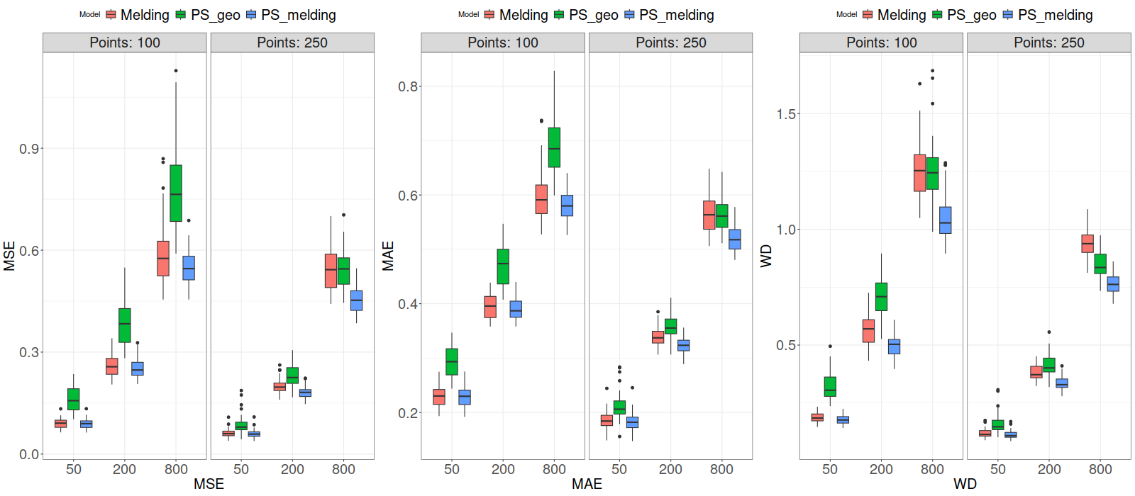
Figure 4: MSE, MAE, and WD values obtained by fitting each of the models when combining 100 or 250 points with 25 areas. Data are simulated under preferential sampling using a value of the microergodic parameter $\theta$ indicated in the horizontal axis.

4.3.2 Parameter estimates

We also evaluate the estimates of the fixed effect and Gaussian random field parameters. Tables 6, 7 and 8 in Supplementary Materials present the average posterior mean, interval scores (Inscore) and 95% coverage probabilities (CP) for the fixed effect $\mu$, the microergodic parameter $\theta$, and the preferential degree $\gamma$ obtained when all models are fitted to several combinations of areal and point data.

When estimating the mean $\mu$, the PSmelding model yields posterior means closer to the true value ($\mu=0$), followed by the PSgeo and Melding model. Fusing reliable areal data results in lower Inscore across scenarios, and increasing the spatial range improves posterior mean estimation of $\mu$. PSmelding consistently performs better on Inscore and CP, with the difference between PSmelding and other models decreasing as spatial range increases. The average posterior mode and credible interval scores are indistinguishable at $\rho=0.4$.

For the microergodic parameter $\theta$, at $\rho=0.4$ and $\theta=50$, the three models show similar performance in posterior mean and credible interval. Sampling size has little influence. At $\rho=0.2$ and $\theta=200$, increasing the number of points decreases the posterior mean. Also, ignoring preferential sampling (Melding) results in wider credible interval. The average posterior mode and CP of PSgeo decrease with more points; on the other hand, Inscore remains stable under the same setting. PSmelding achieves a trade-off between credible interval width and coverage.

At $\rho=0.1$ and $\theta=800$, all models perform worse due to low spatial dependency. PSgeo has low average Inscore and low CP, Melding has high average Inscore and high CP, and PSmelding outperforms, on average, the other approaches (all based on the posterior mode).

Regarding preferential sampling $\gamma$, PSmelding and PSgeo yield similar posterior means for $\gamma$. The 95% credible intervals of PSmelding becomes more precise with more areal data. At $\rho=0.1$, PSmelding recovers $\gamma$ better than PSgeo based on CP and Inscore values.

5 Spatial interpolation of $\text{PM}_{2.5}$ levels in USA

Particulate matter 2.5 ($\text{PM}_{2.5}$) is a type of air pollutant consisting of tiny particles with a diameter of 2.5 microns per cubic meter or less that are suspended in the air. These particles can originate from various sources, including vehicle exhausts, industrial emissions, and natural events such as wildfires. Due to their small size, $\text{PM}_{2.5}$ particles can easily penetrate deep into the lungs and enter the bloodstream leading to adverse health effects including respiratory and cardiovascular diseases and increased mortality rates (Kampa and Castanas, 2008; Di et al., 2017; Thurston et al., 2017).

In the United States of America (USA), the Environmental Protection Agency (EPA) has established National Ambient Air Quality Standards (NAAQS) for $\text{PM}_{2.5}$ to protect public health and the environment. However, despite efforts to control and reduce $\text{PM}_{2.5}$ levels, many areas in the country continue to experience high levels of this harmful pollutant, particularly urban areas and regions with significant industrial activity.

In this section, we fit the proposed spatial misaligned model adjusting for preferential sampling to point and areal level measurements of $\text{PM}_{2.5}$ in the USA in 2019 to predict $\text{PM}_{2.5}$ in a continuous surface. The selected year aims at avoiding the influence of COVID-19. For comparison, we also fit two alternative models, namely, a melding model without adjusting for preferential sampling, and a geostatistical model adjusting by preferential sampling. Figure 5 shows the 498 point data obtained from EPA (United States Environmental Protection Agency, 2019), and the 280 aggregated areal data at a resolution 25 $\times$ 25 degrees from NASA satellites (Hammer et al., 2020, 2022). Preferential sampling in point data may potentially occur as we observe more monitoring sites in areas with high $\text{PM}_{2.5}$ levels, such as the west coast than in areas with low $\text{PM}_{2.5}$ levels, such as the central part of USA. We obtain $\text{PM}_{2.5}$ predictions at 17358 sites to generate a fine surface of the USA.

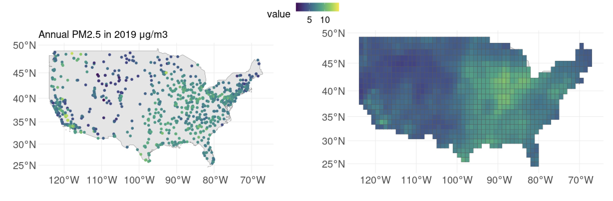
Figure 5: $\text{PM}_{2.5}$ levels in the USA in 2019 obtained at locations of EPA monitoring sites (left) and grid cells generated by NASA satellites (right).

To fit the models, we first project the spatial data which is given in a geographic coordinate reference system into a two-dimensional surface using the Mercator projection with units in kilometers. Then, we create a common mesh to fit all the models using the INLA and SPDE approaches. The dual mesh for estimating the intensity surface of the point process is created using the center of the triangles of the original mesh with the same number of the nodes. In order to obtain reasonable priors for the parameters of the Matérn covariance function of the Gaussian random field, we first fit the model to areal data only. Then, we use the posterior means of the parameters to set priors $\mathbb{P}(\sigma>1.0)=0.01$, and $\mathbb{P}(\rho<934~{}\text{km})=0.90$, and $\nu=1$.

Table 3 shows the estimated parameters and hyperparameters for each of the models fitted. We observe the preferential sampling parameter $\gamma$ is significant both in the PSmelding and PSgeo models as zero is not included in their 95% credible intervals. The PS melding model yields narrower 95% credible intervals for all parameters and hyperparameters than the other two models.

Table 3: Posterior means 95% credible intervals of the parameters and hyperparameters obtained with each of the models.

	PSmelding		PSgeo		Melding
	Mean	95% CI	Mean	95% CI	Mean	95% CI
Intercept $\mu$	6.18	(5.80 , 6.56)	6.15	(5.67 , 6.60)	6.28	(5.84 , 6.71)
Precision for noise $\tau$	0.58	(0.52 , 0.64)	0.34	(0.29, 0.40)	0.59	(0.53, 0.65)
Spatial range $\rho$	706.66	(579.08, 859.98)	801.08	(598.57, 1054.35)	911.37	(705.17, 1164.72)
Standard deviation of GRF $\sigma_{\boldsymbol{\phi}}$	1.06	(0.93, 1.19)	1.49	(1.05, 2.07)	1.01	(0.87 , 1.15)
Preferential sampling $\gamma$	0.50	(0.42, 0.58)	0.71	(0.54, 0.87)	-	-

Maps with the posterior means as well as lower and upper limits of 95% credible intervals obtained with the proposed melding model adjusting for preferential sampling are shown in Figure 6. Similarly, the corresponding results for the two remaining models are presented in the Supplementary Material. In Figure 6, we observe that the annual $\text{PM}_{2.5}$ levels are higher in the Eastern US and California than other regions in the USA. The $\text{PM}_{2.5}$ values in northern Utah and southern Wyoming are slightly higher than other regions in central USA.

Figure 7 displays maps with the exceedance probabilities of $\text{PM}_{2.5}$ levels being larger than 8 microns per cubic meter obtained with each of the models. We observe different spatial patterns of exceedance probabilities obtained with each of the models. With the melding model, exceedance probabilities are high in most locations of the east. On the other hand, both models that assume preferential sampling show lower probabilities in southeastern region covering states such as Mississippi and Louisiana.

Both maps of air pollution estimates and exceedance probabilities may be used to inform decision-making by identifying locations of high air pollution where intervention measures need to be taken. Therefore, it is important to be able to specify models that can account for preferential sampling in order to avoid wrong inferences that may influence decisions and allocation of resources in areas where they are not needed.

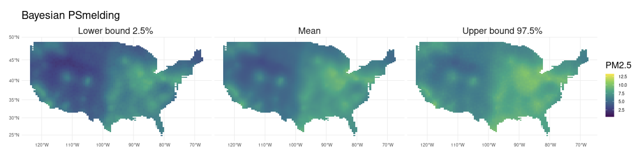
Figure 6: $\text{PM}_{2.5}$ levels in the USA in 2019 interpolated using the PSmelding model.

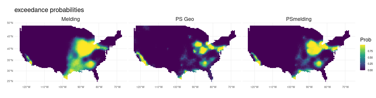
Figure 7: Exceedance probabilities that $\text{PM}_{2.5}$ levels are higher than 8 microns per cubic meter obtained with each of the models.

6 Discussion

In this paper, we propose a Bayesian hierarchical model to combine spatially misaligned data adjusting for preferential sampling. This approach specifies a Bayesian melding model that fuses data available at different spatial resolutions by assuming a common Gaussian random field underlying all observations. The model accounts for preferential sampling by assuming that the Gaussian random field used to model the observations is shared with the log intensity of the point process that originates the locations. A scale parameter is used to control the level of preferential degree. The model is implemented using the data fusion procedure proposed by Moraga et al. (2017) with the INLA and SPDE approaches, which presents computational advantages compared to MCMC methods.

By means of a simulation study, we show that the model that combines point- and areal-level data accounting for preferential sampling outperforms models that just use one type of data or combine data without accounting for preferential sampling. Specifically, we observe that the model that combines data ignoring preferential sampling yields higher MSE, MAE, and WD values, especially when smaller amount of areal data are available. Also, our model presents better performance (according to these error measures) than the model that accounts for preferential sampling but just use point-level data.

In terms of the parameter estimation, ignoring preferential sampling leads to an unreliable fixed effect posterior mean when areal data are limited, with low coverage probabilities and narrower credible intervals. Our model outperforms other models regarding the obtained posterior mean and credible intervals. As for the hyperparameters, when the spatial dependence is not strong, our model leads to a trade-off between a narrow credible intervals and the ability of covering the true value, whereas the model that just utilizes point-level data tends to have a narrower interval but low CP, and the melding model that does not adjust for preferential sampling presents a wider interval with a higher CP. Comparing the average posterior mean, our model outperforms the other two models.

We also apply our model to predict $\text{PM}_{2.5}$ levels in the USA in 2019. The significant preferential degree gives us evidence that the sampling scheme for the monitoring sites might be preferential. This needs to be taken into account when fitting a model to the data in order to obtain valid inferences.

Our proposed model is flexible and can be extended in a number of ways. For example, we could include different structures for the fixed effects, as well as additional random effects to account for different sources of variability. The estimation of the extended model in this way can utilize the estimation of the latent Gaussian random field using the INLA and SPDE approaches. We can also extend the proposed model by considering a non-Gaussian non-stationary responses. Cabral et al. (2022) and Bolin et al. (2023) describe how the INLA and SPDE approaches can be extended to the non-Gaussian case. Vihrs et al. (2022) proposed a log Gaussian Cox Strauss process for random repulsion and regression in point patterns—that could be also further investigated in the preferential sampling melding model.

The model presented has been used to combine spatially misaligned data adjusting for preferential sampling. This model can also be used to analyze spatio-temporal data that could be available at different spatial and temporal resolutions. In these situations, we could assume that underlying all observations there is a spatio-temporal Gaussian random field. Then, data aggregated in time, space or space-time could be considered as averages of the Gaussian process at the available resolution. To account for preferential sampling, the latent Gaussian random field will also be shared by the log intensity of the point process that generates the sampling locations. The scaling parameter that modulates the preferential degree can be considered fixed or varying in space and/or time.

In summary, our work allows for the fusion of spatial data available at different resolutions, while also accounting for the possible dependence between the sampling scheme and the underlying process. Our proposed fitting procedure presents computational advantages over MCMC-based methods, as it relies on faster inference techniques. Our model was shown to work well under different (and sometimes, misspecified) scenarios—both for spatial interpolation and parameters estimation. Thus, although possible to extend, our work presents a first attempt to model spatially misaligned data under the assumption of preferential sampling.

7 Declarations of interest

Declarations of interest: none

Supplementary Material

Table 4: Mean of the scores and 95% quantile intervals obtained with Melding, PSmelding and PSgeo models in scenarios generated with different values of the spatial range $\rho$. Scenarios combine 100 point observations with 0, 4, 25 or 100 areas under preferential sampling and non-preferential sampling settings. Results obtained PSgeo model do not include areal data, the value of areas indicates the corresponding simulation data.

			Preferential sampling			Non-preferential sampling
Model	Areas	$\rho$	MSE	MAE	WD	MSE	MAE	WD
Melding	4	0.1	1.05 (0.69 1.41)	0.8 (0.65 0.94)	1.6 (1.33 1.96)	0.74 (0.61 0.89)	0.67 (0.62 0.74)	1.4 (1.1 1.81)
Melding	4	0.2	0.47 (0.3 0.83)	0.52 (0.42 0.68)	0.84 (0.65 1.11)	0.39 (0.3 0.56)	0.48 (0.43 0.56)	0.8 (0.63 1.07)
Melding	4	0.4	0.15 (0.1 0.25)	0.29 (0.24 0.35)	0.31 (0.21 0.47)	0.18 (0.13 0.31)	0.33 (0.28 0.42)	0.43 (0.32 0.63)
Melding	25	0.1	0.59 (0.47 0.86)	0.6 (0.53 0.74)	1.26 (1.06 1.57)	0.67 (0.56 0.78)	0.64 (0.59 0.69)	1.27 (1.04 1.62)
Melding	25	0.2	0.26 (0.21 0.33)	0.39 (0.36 0.44)	0.56 (0.44 0.72)	0.34 (0.26 0.46)	0.46 (0.4 0.52)	0.71 (0.57 0.88)
Melding	25	0.4	0.09 (0.07 0.12)	0.23 (0.2 0.27)	0.19 (0.15 0.23)	0.15 (0.11 0.21)	0.3 (0.26 0.36)	0.37 (0.31 0.46)
Melding	100	0.1	0.38 (0.34 0.45)	0.48 (0.46 0.53)	0.83 (0.68 1.01)	0.48 (0.42 0.55)	0.55 (0.52 0.59)	0.95 (0.83 1.09)
Melding	100	0.2	0.14 (0.11 0.17)	0.29 (0.26 0.32)	0.28 (0.24 0.34)	0.22 (0.18 0.25)	0.37 (0.33 0.4)	0.47 (0.41 0.55)
Melding	100	0.4	0.04 (0.03 0.05)	0.16 (0.14 0.18)	0.08 (0.07 0.1)	0.1 (0.08 0.13)	0.25 (0.22 0.29)	0.27 (0.24 0.33)
PSgeo	4	0.1	0.78 (0.61 1)	0.69 (0.61 0.8)	1.27 (1.07 1.52)	0.76 (0.62 0.98)	0.68 (0.62 0.78)	1.44 (1.15 1.82)
PSgeo	4	0.2	0.4 (0.27 0.6)	0.48 (0.4 0.58)	0.71 (0.56 0.9)	0.41 (0.31 0.61)	0.49 (0.44 0.58)	0.84 (0.65 1.17)
PSgeo	4	0.4	0.16 (0.1 0.36)	0.29 (0.24 0.4)	0.31 (0.22 0.62)	0.19 (0.13 0.32)	0.33 (0.28 0.42)	0.45 (0.33 0.64)
PSgeo	25	0.1	0.78 (0.6 1.11)	0.69 (0.61 0.83)	1.25 (1.03 1.67)	0.77 (0.63 0.99)	0.69 (0.62 0.78)	1.44 (1.02 1.92)
PSgeo	25	0.2	0.39 (0.28 0.54)	0.47 (0.41 0.55)	0.71 (0.54 0.89)	0.42 (0.29 0.57)	0.5 (0.43 0.57)	0.85 (0.66 1.04)
PSgeo	25	0.4	0.16 (0.11 0.23)	0.29 (0.24 0.35)	0.32 (0.24 0.47)	0.19 (0.12 0.31)	0.33 (0.28 0.4)	0.44 (0.32 0.6)
PSgeo	100	0.1	0.76 (0.57 1.05)	0.68 (0.59 0.81)	1.27 (1 1.67)	0.73 (0.63 0.87)	0.67 (0.62 0.74)	1.44 (1.14 1.79)
PSgeo	100	0.2	0.39 (0.29 0.59)	0.47 (0.41 0.57)	0.72 (0.54 0.92)	0.41 (0.32 0.58)	0.49 (0.44 0.58)	0.83 (0.64 1.05)
PSgeo	100	0.4	0.16 (0.09 0.27)	0.29 (0.23 0.35)	0.32 (0.21 0.53)	0.18 (0.12 0.23)	0.33 (0.27 0.37)	0.43 (0.33 0.56)
PSmelding	4	0.1	0.68 (0.55 0.85)	0.65 (0.58 0.73)	1.22 (1.03 1.45)	0.75 (0.62 0.92)	0.68 (0.62 0.76)	1.38 (1.09 1.77)
PSmelding	4	0.2	0.35 (0.26 0.47)	0.45 (0.39 0.53)	0.66 (0.54 0.78)	0.4 (0.3 0.6)	0.49 (0.43 0.59)	0.8 (0.63 1.09)
PSmelding	4	0.4	0.14 (0.09 0.23)	0.28 (0.24 0.35)	0.27 (0.2 0.42)	0.19 (0.13 0.3)	0.33 (0.28 0.42)	0.43 (0.33 0.62)
PSmelding	25	0.1	0.55 (0.46 0.67)	0.58 (0.53 0.63)	1.05 (0.9 1.28)	0.67 (0.56 0.79)	0.64 (0.59 0.7)	1.24 (1.01 1.64)
PSmelding	25	0.2	0.26 (0.21 0.33)	0.39 (0.36 0.44)	0.5 (0.4 0.61)	0.34 (0.25 0.46)	0.46 (0.4 0.52)	0.7 (0.57 0.85)
PSmelding	25	0.4	0.09 (0.07 0.12)	0.23 (0.2 0.27)	0.18 (0.14 0.22)	0.15 (0.11 0.21)	0.3 (0.26 0.36)	0.36 (0.31 0.46)
PSmelding	100	0.1	0.38 (0.34 0.44)	0.48 (0.46 0.52)	0.71 (0.61 0.88)	0.48 (0.42 0.55)	0.55 (0.51 0.59)	0.94 (0.82 1.11)
PSmelding	100	0.2	0.14 (0.11 0.17)	0.29 (0.26 0.32)	0.27 (0.22 0.31)	0.22 (0.18 0.25)	0.37 (0.33 0.4)	0.47 (0.41 0.55)
PSmelding	100	0.4	0.04 (0.03 0.05)	0.16 (0.14 0.18)	0.08 (0.07 0.1)	0.1 (0.08 0.13)	0.25 (0.22 0.29)	0.27 (0.24 0.32)

Table 5: Mean of the scores and 95% quantile intervals obtained with Melding, PSmelding and PSgeo models in scenarios generated with different values of the spatial range $\rho$. Scenarios combine 250 point observations with 0, 4, 25 or 100 areas under preferential sampling and non-preferential sampling settings. Results obtained PSgeo model do not include areal data, the value of areas indicates the corresponding simulation data.

			Preferential sampling			Non-preferential sampling
Model	Areas	$\rho$	MSE	MAE	WD	MSE	MAE	WD
Melding	4	0.1	0.83 (0.62 1.06)	0.69 (0.61 0.78)	1.21 (1.02 1.39)	0.51 (0.43 0.65)	0.55 (0.5 0.62)	0.96 (0.81 1.09)
Melding	4	0.2	0.31 (0.2 0.47)	0.41 (0.33 0.49)	0.53 (0.38 0.74)	0.23 (0.17 0.26)	0.37 (0.33 0.4)	0.49 (0.42 0.57)
Melding	4	0.4	0.09 (0.05 0.14)	0.21 (0.17 0.26)	0.17 (0.11 0.23)	0.09 (0.07 0.12)	0.24 (0.21 0.27)	0.27 (0.23 0.31)
Melding	25	0.1	0.55 (0.45 0.7)	0.57 (0.51 0.64)	0.94 (0.83 1.06)	0.49 (0.43 0.58)	0.54 (0.51 0.59)	0.93 (0.81 1.08)
Melding	25	0.2	0.2 (0.16 0.26)	0.34 (0.31 0.38)	0.38 (0.32 0.45)	0.22 (0.18 0.26)	0.36 (0.33 0.39)	0.48 (0.42 0.55)
Melding	25	0.4	0.06 (0.04 0.1)	0.19 (0.15 0.23)	0.12 (0.09 0.17)	0.09 (0.07 0.11)	0.23 (0.21 0.26)	0.26 (0.23 0.29)
Melding	100	0.1	0.34 (0.3 0.4)	0.45 (0.43 0.49)	0.65 (0.58 0.74)	0.4 (0.34 0.46)	0.5 (0.46 0.53)	0.76 (0.67 0.88)
Melding	100	0.2	0.12 (0.1 0.14)	0.27 (0.24 0.29)	0.23 (0.19 0.27)	0.17 (0.14 0.21)	0.33 (0.3 0.35)	0.4 (0.35 0.45)
Melding	100	0.4	0.04 (0.03 0.04)	0.14 (0.13 0.16)	0.07 (0.06 0.08)	0.07 (0.06 0.08)	0.21 (0.19 0.23)	0.23 (0.21 0.25)
PSgeo	4	0.1	0.55 (0.45 0.74)	0.57 (0.52 0.66)	0.84 (0.74 0.97)	0.51 (0.43 0.65)	0.55 (0.51 0.63)	0.95 (0.8 1.09)
PSgeo	4	0.2	0.24 (0.17 0.32)	0.36 (0.31 0.41)	0.41 (0.32 0.54)	0.23 (0.17 0.26)	0.37 (0.33 0.4)	0.49 (0.43 0.57)
PSgeo	4	0.4	0.08 (0.05 0.14)	0.2 (0.17 0.26)	0.15 (0.11 0.23)	0.1 (0.07 0.12)	0.24 (0.21 0.28)	0.27 (0.23 0.31)
PSgeo	25	0.1	0.54 (0.45 0.68)	0.56 (0.51 0.64)	0.84 (0.74 0.96)	0.51 (0.44 0.6)	0.55 (0.52 0.6)	0.95 (0.82 1.12)
PSgeo	25	0.2	0.23 (0.17 0.3)	0.36 (0.31 0.41)	0.41 (0.32 0.53)	0.23 (0.2 0.27)	0.37 (0.34 0.4)	0.5 (0.44 0.58)
PSgeo	25	0.4	0.09 (0.05 0.18)	0.21 (0.17 0.28)	0.16 (0.11 0.3)	0.09 (0.07 0.12)	0.24 (0.21 0.26)	0.27 (0.24 0.3)
PSgeo	100	0.1	0.54 (0.43 0.63)	0.56 (0.51 0.61)	0.85 (0.72 0.93)	0.52 (0.42 0.64)	0.56 (0.51 0.61)	0.95 (0.81 1.18)
PSgeo	100	0.2	0.23 (0.17 0.34)	0.36 (0.31 0.43)	0.41 (0.32 0.55)	0.23 (0.18 0.29)	0.37 (0.34 0.41)	0.5 (0.44 0.59)
PSgeo	100	0.4	0.08 (0.06 0.14)	0.21 (0.17 0.26)	0.16 (0.12 0.27)	0.09 (0.07 0.12)	0.24 (0.21 0.26)	0.27 (0.24 0.31)
PSmelding	4	0.1	0.53 (0.44 0.7)	0.56 (0.51 0.64)	0.83 (0.74 0.96)	0.51 (0.43 0.65)	0.55 (0.5 0.62)	0.96 (0.81 1.09)
PSmelding	4	0.2	0.23 (0.16 0.29)	0.36 (0.31 0.4)	0.4 (0.32 0.51)	0.23 (0.17 0.26)	0.37 (0.33 0.4)	0.49 (0.42 0.57)
PSmelding	4	0.4	0.08 (0.05 0.13)	0.2 (0.17 0.25)	0.15 (0.1 0.22)	0.1 (0.07 0.12)	0.24 (0.21 0.28)	0.27 (0.23 0.31)
PSmelding	25	0.1	0.45 (0.39 0.53)	0.52 (0.48 0.57)	0.77 (0.68 0.86)	0.49 (0.43 0.58)	0.54 (0.51 0.59)	0.93 (0.81 1.08)
PSmelding	25	0.2	0.18 (0.15 0.22)	0.32 (0.3 0.36)	0.33 (0.28 0.4)	0.22 (0.18 0.26)	0.36 (0.33 0.39)	0.48 (0.42 0.55)
PSmelding	25	0.4	0.06 (0.04 0.1)	0.18 (0.15 0.23)	0.11 (0.09 0.16)	0.09 (0.07 0.11)	0.23 (0.21 0.26)	0.26 (0.23 0.29)
PSmelding	100	0.1	0.33 (0.29 0.39)	0.45 (0.42 0.48)	0.58 (0.52 0.65)	0.4 (0.34 0.46)	0.5 (0.46 0.53)	0.76 (0.67 0.88)
PSmelding	100	0.2	0.12 (0.1 0.14)	0.27 (0.24 0.29)	0.22 (0.18 0.25)	0.17 (0.14 0.21)	0.33 (0.3 0.35)	0.4 (0.35 0.45)
PSmelding	100	0.4	0.04 (0.03 0.04)	0.14 (0.13 0.16)	0.07 (0.06 0.08)	0.07 (0.06 0.08)	0.21 (0.19 0.23)	0.23 (0.21 0.25)

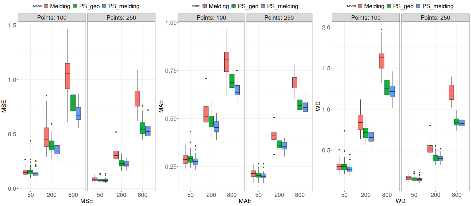
Figure 8: MSE, MAE, and WD values obtained by fitting each of the models when combining 100 or 250 points with 4 (top) and 100 (bottom) areas. Data are simulated under preferential sampling using a value of the microergodic parameter $\theta$ indicated in the horizontal axis.

Table 6: Average posterior mean, interval score (Inscore) and 95% coverage probability (CP) for the fixed effect $\mu$ (top), the microergodic parameter $\theta$ (middle), and the preferential sampling $\gamma$ (bottom) obtained with each model. Models are fitted to several combinations of areal and point data generated with $\mu=0$, $\theta=200$ and $\gamma=1$ indicating preferential sampling and spatial correlation $\rho=0.2$.

$\mu=0$		PSmelding			Melding			PSgeo
Areas	Points	Mean	Inscore	CP	Mean	Inscore	CP	Mean	Inscore	CP
4	100	0.05	0.03	0.94	0.26	0.05	0.82	0.11	0.03	0.93
4	250	0.07	0.03	0.90	0.26	0.06	0.65	0.09	0.03	0.90
25	100	0.02	0.03	0.92	0.06	0.03	0.91	0.07	0.03	0.93
25	250	0.05	0.03	0.94	0.13	0.03	0.86	0.10	0.03	0.90
100	100	0.02	0.03	0.91	0.03	0.03	0.91	0.10	0.03	0.88
100	250	0.03	0.03	0.91	0.06	0.03	0.91	0.08	0.03	0.88
$\theta=200$
4	100	193.36	125.70	0.89	179.12	128.58	0.87	177.12	112.69	0.84
4	250	163.05	117.06	0.75	185.87	127.98	0.89	157.89	112.92	0.69
25	100	202.05	135.62	0.85	251.55	161.11	0.79	177.60	113.72	0.84
25	250	169.44	123.04	0.77	183.39	128.37	0.93	152.73	108.87	0.62
100	100	189.59	135.03	0.83	222.68	154.06	0.82	179.84	114.31	0.81
100	250	171.58	128.24	0.74	190.49	138.12	0.90	154.23	110.19	0.62
$\gamma=1$
4	100	0.85	0.67	0.65				0.84	0.65	0.63
4	250	0.86	0.74	0.46				0.87	0.74	0.46
25	100	0.88	0.71	0.75				0.86	0.67	0.73
25	250	0.88	0.76	0.60				0.88	0.75	0.58
100	100	0.91	0.74	0.85				0.86	0.66	0.74
100	250	0.90	0.78	0.70				0.88	0.76	0.61

Table 7: Average posterior mean, interval score (Inscore) and 95% coverage probability (CP) for the fixed effect $\mu$ (top), the microergodic parameter $\theta$ (middle), and the preferential sampling $\gamma$ (bottom) obtained with each model. Models are fitted to several combinations of areal and point data generated with $\mu=0$, $\theta=800$ and $\gamma=1$ indicating preferential sampling and spatial correlation $\rho=0.1$.

$\mu=0$		PSmelding			Melding			PSgeo
Areas	Points	Mean	Inscore	CP	Mean	Inscore	CP	Mean	Inscore	CP
4	100	0.13	0.02	0.92	0.55	0.24	0.12	0.28	0.06	0.66
4	250	0.18	0.03	0.80	0.49	0.27	0.04	0.21	0.04	0.72
25	100	0.03	0.02	0.93	0.13	0.03	0.80	0.30	0.06	0.65
25	250	0.09	0.02	0.89	0.28	0.09	0.42	0.20	0.05	0.71
100	100	0.00	0.02	0.85	0.02	0.02	0.82	0.28	0.07	0.65
100	250	0.04	0.02	0.89	0.10	0.03	0.75	0.20	0.05	0.69
$\theta=800$
4	100	552.30	321.44	0.74	544.99	345.35	0.88	484.49	274.47	0.61
4	250	471.11	306.41	0.38	726.40	413.00	0.92	442.05	286.40	0.36
25	100	856.12	520.50	0.80	1263.07	718.07	0.65	550.52	310.64	0.53
25	250	565.87	375.05	0.56	666.71	402.50	0.87	441.26	287.31	0.35
100	100	922.31	598.74	0.80	1570.56	969.80	0.53	562.73	323.58	0.55
100	250	662.34	446.39	0.76	913.56	560.15	0.89	419.13	270.20	0.25
$\gamma=1$
4	100	0.75	0.56	0.33				0.72	0.50	0.33
4	250	0.76	0.63	0.11				0.76	0.63	0.12
25	100	0.77	0.60	0.32				0.73	0.50	0.39
25	250	0.76	0.65	0.07				0.76	0.63	0.09
100	100	0.82	0.66	0.58				0.71	0.50	0.40
100	250	0.79	0.68	0.09				0.78	0.65	0.15

Table 8: Average posterior mean, interval score (Inscore) and 95% coverage probability (CP) for the fixed effect $\mu$ (top), the microergodic parameter $\theta$ (middle), and the preferential sampling $\gamma$ (bottom) obtained with each model. Models are fitted to several combinations of areal and point data generated with $\mu=0$, $\theta=50$ and $\gamma=1$ indicating preferential sampling and spatial correlation $\rho=0.4$.

$\mu=0$		PSmelding			Melding			PSgeo
Areas	Points	Mean	Inscore	CP	Mean	Inscore	CP	Mean	Inscore	CP
4	100	-0.02	0.04	0.91	0.05	0.04	0.91	0.00	0.04	0.95
4	250	0.02	0.05	0.85	0.11	0.06	0.82	0.02	0.05	0.85
25	100	-0.00	0.05	0.85	0.02	0.05	0.85	0.04	0.05	0.91
25	250	0.02	0.04	0.84	0.05	0.04	0.84	0.04	0.04	0.87
100	100	-0.00	0.04	0.84	0.01	0.05	0.84	0.03	0.05	0.87
100	250	0.00	0.05	0.84	0.02	0.05	0.80	0.01	0.05	0.87
$\theta=50$
4	100	52.39	35.50	0.89	51.56	34.43	0.91	50.89	34.68	0.87
4	250	44.43	33.08	0.85	45.46	33.56	0.89	43.63	32.43	0.82
25	100	49.21	34.17	0.95	52.32	34.96	0.95	47.52	31.23	0.93
25	250	47.54	36.04	0.85	48.69	36.56	0.87	45.87	34.22	0.78
100	100	47.50	35.56	0.84	49.14	36.37	0.85	50.48	34.31	0.95
100	250	45.52	35.18	0.87	46.69	35.85	0.89	45.05	33.50	0.89
$\gamma=1$
4	100	0.95	0.75	0.91				0.95	0.74	0.95
4	250	0.94	0.81	0.82				0.94	0.81	0.85
25	100	0.97	0.77	0.95				0.96	0.75	0.96
25	250	0.93	0.80	0.85				0.93	0.80	0.82
100	100	0.98	0.78	0.93				0.96	0.75	0.95
100	250	0.94	0.81	0.95				0.93	0.80	0.91

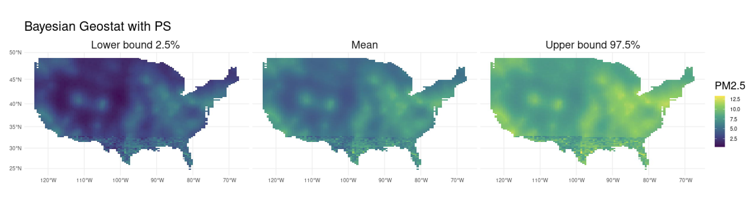
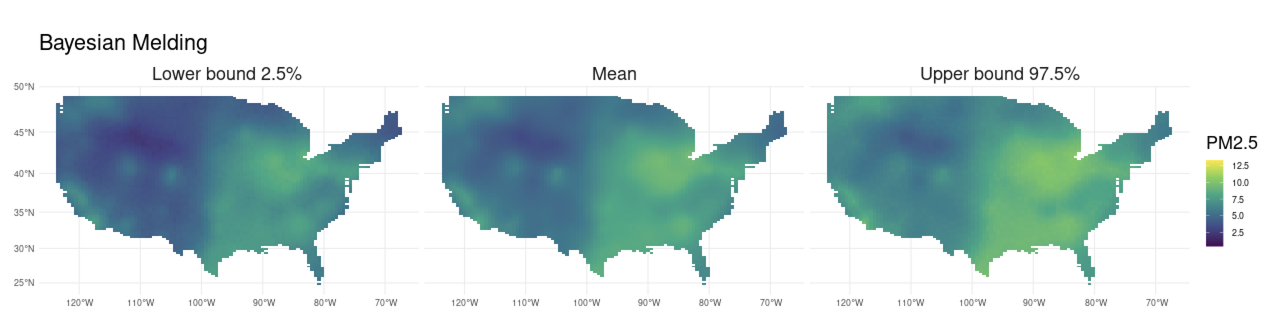
Figure 9: $\text{PM}{2.5}$ levels in the USA in 2019 interpolated using the PSgeo (top) and Melding (bottom) models.

References

- Baddeley and Turner (2000) Baddeley, A., Turner, R., 2000. Practical maximum pseudolikelihood for spatial point patterns: (with discussion). Australian & New Zealand Journal of Statistics 42, 283–322.
- Berrocal et al. (2010) Berrocal, V.J., Gelfand, A.E., Holland, D.M., 2010. A spatio-temporal downscaler for output from numerical models. Journal of Agricultural, Biological, and Environmental Statistics 15. doi:10.1007/s13253-009-0004-z.
- Bolin et al. (2023) Bolin, D., Jin, X., Simas, A., Wallin, J., 2023. ngme2: Latent Mixed Effects Models With Flexible Distributions. URL: https://davidbolin.github.io/ngme2/. r package version 0.3.0.
- Cabral et al. (2022) Cabral, R., Bolin, D., Rue, H., 2022. Fitting latent non-gaussian models using variational bayes and laplace approximations. arXiv preprint arXiv:2211.11050 .
- Cappello and Palacios (2022) Cappello, L., Palacios, J.A., 2022. Adaptive preferential sampling in phylodynamics with an application to sars-cov-2. Journal of Computational and Graphical Statistics 31, 541–552.
- Cecconi et al. (2016) Cecconi, L., Grisotto, L., Catelan, D., Lagazio, C., Berrocal, V., Biggeri, A., 2016. Preferential sampling and bayesian geostatistics: Statistical modeling and examples. Statistical methods in medical research 25, 1224–1243.
- Conn et al. (2017) Conn, P.B., Thorson, J.T., Johnson, D.S., 2017. Confronting preferential sampling when analysing population distributions: diagnosis and model-based triage. Methods in Ecology and Evolution 8, 1535–1546.
- Cox (1955) Cox, D.R., 1955. Some statistical methods connected with series of events. Journal of the Royal Statistical Society: Series B (Methodological) 17, 129–157.
- Di et al. (2017) Di, Q., Wang, Y., Zanobetti, A., Wang, Y., Koutrakis, P., Choirat, C., Dominici, F., Schwartz, J.D., 2017. Air pollution and mortality in the medicare population. New England Journal of Medicine 376, 2513–2522.
- Diggle et al. (2010) Diggle, P.J., Menezes, R., Su, T.l., 2010. Geostatistical inference under preferential sampling. Journal of the Royal Statistical Society: Series C (Applied Statistics) 59, 191–232.
- Dinsdale et al. (2019) Dinsdale, D., Salibian-Barrera, M., et al., 2019. Methods for preferential sampling in geostatistics. Journal of the Royal Statistical Society Series C 68, 181–198.
- Engquist and Froese (2013) Engquist, B., Froese, B.D., 2013. Application of the wasserstein metric to seismic signals. arXiv preprint arXiv:1311.4581 .
- Fuentes and Raftery (2005) Fuentes, M., Raftery, A.E., 2005. Model evaluation and spatial interpolation by bayesian combination of observations with outputs from numerical models. Biometrics 61, 36–45.
- Givens and Shortt (1984) Givens, C.R., Shortt, R.M., 1984. A class of wasserstein metrics for probability distributions. Michigan Mathematical Journal 31, 231–240.
- Gneiting and Raftery (2007) Gneiting, T., Raftery, A.E., 2007. Strictly proper scoring rules, prediction, and estimation. Journal of the American statistical Association 102, 359–378.
- Hammer et al. (2022) Hammer, M.S., van Donkelaar, A., Li, C., Lyapustin, A., Sayer, A.M., Hsu, N.C., Levy, R.C., Garay, M.J., Kalashnikova, O.V., Kahn, R.A., Brauer, M., Apte, J.S., Henze, D.K., Zhang, L., Zhang, Q., Ford, B., 2022. Global annual pm2.5 grids from modis, misr and seawifs aerosol optical depth (aod), 1998-2019, v4.gl.03 URL: https://doi.org/10.7927/fx80-4n39.
- Hammer et al. (2020) Hammer, M.S., van Donkelaar, A., Li, C., Lyapustin, A., Sayer, A.M., Hsu, N.C., Levy, R.C., Garay, M.J., Kalashnikova, O.V., Kahn, R.A., et al., 2020. Global estimates and long-term trends of fine particulate matter concentrations (1998–2018). Environmental Science & Technology 54, 7879–7890.
- Illian et al. (2012) Illian, J.B., Sørbye, S.H., Rue, H., 2012. A toolbox for fitting complex spatial point process models using integrated nested laplace approximation (inla) .
- Kampa and Castanas (2008) Kampa, M., Castanas, E., 2008. Human health effects of air pollution. Environmental pollution 151, 362–367.
- Kantorovich (1960) Kantorovich, L.V., 1960. Mathematical methods of organizing and planning production. Management science 6, 366–422.
- Krainski et al. (2018) Krainski, E., Gómez-Rubio, V., Bakka, H., Lenzi, A., Castro-Camilo, D., Simpson, D., Lindgren, F., Rue, H., 2018. Advanced spatial modeling with stochastic partial differential equations using R and INLA. Chapman and Hall/CRC.
- Lindgren et al. (2011) Lindgren, F., Rue, H., Lindström, J., 2011. An explicit link between gaussian fields and gaussian markov random fields: the stochastic partial differential equation approach. Journal of the Royal Statistical Society: Series B (Statistical Methodology) 73, 423–498.
- Mohajerin Esfahani and Kuhn (2018) Mohajerin Esfahani, P., Kuhn, D., 2018. Data-driven distributionally robust optimization using the wasserstein metric: Performance guarantees and tractable reformulations. Mathematical Programming 171, 115–166.
- Møller et al. (1998) Møller, J., Syversveen, A.R., Waagepetersen, R.P., 1998. Log gaussian cox processes. Scandinavian journal of statistics 25, 451–482.
- Moraga et al. (2017) Moraga, P., Cramb, S.M., Mengersen, K.L., Pagano, M., 2017. A geostatistical model for combined analysis of point-level and area-level data using inla and spde. Spatial Statistics 21. doi:10.1016/j.spasta.2017.04.006.
- Pati et al. (2011) Pati, D., Reich, B.J., Dunson, D.B., 2011. Bayesian geostatistical modelling with informative sampling locations. Biometrika 98, 35–48.
- Rue et al. (2009) Rue, H., Martino, S., Chopin, N., 2009. Approximate bayesian inference for latent gaussian models by using integrated nested laplace approximations. Journal of the royal statistical society: Series b (statistical methodology) 71, 319–392.
- Rue et al. (2017) Rue, H., Riebler, A., Sørbye, S.H., Illian, J.B., Simpson, D.P., Lindgren, F.K., 2017. Bayesian computing with inla: a review. Annual Review of Statistics and Its Application 4, 395–421.
- Shirota and Gelfand (2022) Shirota, S., Gelfand, A.E., 2022. Preferential sampling for bivariate spatial data. Spatial Statistics 51, 100674.
- Simpson et al. (2016) Simpson, D., Illian, J.B., Lindgren, F., Sørbye, S.H., Rue, H., 2016. Going off grid: Computationally efficient inference for log-gaussian cox processes. Biometrika 103, 49–70.
- Sun et al. (2022) Sun, Y., Qiu, R., Sun, M., 2022. Optimizing decisions for a dual-channel retailer with service level requirements and demand uncertainties: A wasserstein metric-based distributionally robust optimization approach. Computers & Operations Research 138, 105589.
- Thurston et al. (2017) Thurston, G.D., Kipen, H., Annesi-Maesano, I., Balmes, J., Brook, R.D., Cromar, K., De Matteis, S., Forastiere, F., Forsberg, B., Frampton, M.W., et al., 2017. A joint ers/ats policy statement: what constitutes an adverse health effect of air pollution? an analytical framework. European Respiratory Journal 49.
- United States Environmental Protection Agency (2019) United States Environmental Protection Agency, 2019. Pre-Generated Data Files. https://aqs.epa.gov/aqsweb/airdata/download_files.html.
- Vihrs et al. (2022) Vihrs, N., Møller, J., Gelfand, A.E., 2022. Approximate bayesian inference for a spatial point process model exhibiting regularity and random aggregation. Scandinavian Journal of Statistics 49, 185–210.
- Whittle (1963) Whittle, P., 1963. Stochastic-processes in several dimensions. Bulletin of the International Statistical Institute 40, 974–994.
- Zhang (2004) Zhang, H., 2004. Inconsistent estimation and asymptotically equal interpolations in model-based geostatistics. Journal of the American Statistical Association 99, 250–261.
- Zhao and Guan (2018) Zhao, C., Guan, Y., 2018. Data-driven risk-averse stochastic optimization with wasserstein metric. Operations Research Letters 46, 262–267.