EGIC: Enhanced Low-Bit-Rate Generative Image Compression
Guided by Semantic Segmentation

Abstract

We introduce EGIC, a novel generative image compression method that allows traversing the distortion-perception curve efficiently from a single model. Specifically, we propose an implicitly encoded variant of image interpolation that predicts the residual between a MSE-optimized and GAN-optimized decoder output. On the receiver side, the user can then control the impact of the residual on the GAN-based reconstruction. Together with improved GAN-based building blocks, EGIC outperforms a wide-variety of perception-oriented and distortion-oriented baselines, including HiFiC, MRIC and DIRAC, while performing almost on par with VTM-20.0 on the distortion end. EGIC is simple to implement, very lightweight (e.g. $0.18\times$ model parameters compared to HiFiC) and provides excellent interpolation characteristics, which makes it a promising candidate for practical applications targeting the low bit range.

1 Introduction

Figure 1: Distortion-perception comparison. Top left is better.

Figure 2: Visual comparison of distortion-oriented (blue) and perception-oriented codecs (green). MRIC [1], DIRAC [16] and our method allow traversing the distortion-perception curve from a single model on the receiver side. Best viewed electronically.

Neural image compression methods incorporating generative models (e.g. Generative Adversarial Networks, short GANs [17]) have been able to achieve comparable perceptual quality at significantly lower bit-rates [3, 34], hence being a promising direction for storage-efficient and bandwidth-constrained applications. Its underlying principle is that missing information can be realistically synthesized (e.g. textures), therefore allowing more control over highly-sensitive information.

Formally, these methods fall into the category of lossy compression with high perception  [7, 59, 63], i.e. we are interested in the lowest possible distortion for a given bit-rate with the constraint that the reconstructions follow the underlying data distribution. Note that this definition implies that low distortion alone does not per se yield good perceptual quality. In fact, it has been shown that perception and distortion are at odds with each other [7]. This is especially evident at low bit-rates, where codec-specific artifacts become visible (e.g. blocking artifacts in JPEG). On the other hand, users might worry that the GAN-based reconstructions deviate too much from the original image [1]. For this reason, it is desirable to allow for a dynamic trade-off on the receiver side based on application-dependent preferences.

In this work we introduce EGIC, a novel generative image compression method that allows traversing the distortion-perception (D-P) curve efficiently from a single model. Specifically, we propose an implicitly encoded variant of image interpolation [25, 63] based on transfer learning that predicts the residual between a MSE-optimized and GAN-optimized decoder output. On the receiver side, we can then navigate the D-P trade-off by controlling the impact of the residual on the GAN-based reconstruction ($\alpha\in[0,1]$), as demonstrated in Fig. 1. We further propose several improvements to the semantic segmentation-guided discriminator OASIS [48], which we adopt as a drop-in replacement for the omnipresent PatchGAN discriminator [24]. Specifically, we propose to replace spectral norm [36] with weight norm [44] combined with discriminator pre-training, which we have found to allow for a better model capacity/ training stability trade-off, leading to superior compression performance. Our contributions are:

1. We propose a novel generative image compression method that allows traversing the D-P curve efficiently from a single model (Sec. 4). Our approach is simple and lightweight by design; e.g. compared to MRIC [1], we only require $400$k additional parameters ($0.15\times$).

2. We conduct a thorough study to identify suitable discriminator architectures/ GAN formulations for the task of generative image compression (Sec. 5).

3. We empirically evaluate the effectiveness of our method on HiFiC [34] and SwinT-ChARM [66] on three challenging benchmark datasets (Sec. 6). We find that EGIC is particularly well-suited for the low bit range; e.g. EGIC outperforms HiFiC-lo, even when using $30$% fewer bits. EGIC also outperforms MRIC and DIRAC [16], while being significantly more storage-efficient ($0.18-0.55\times$ model parameters).

2 Related work

Generative image compression. Motivated by the success of pix2pixHD [56], Agustsson et al. [3] proposed an extreme learned image compression method ($<0.1$bpp). Specifically, an entropy-constrained convolutional auto-encoder with a multi-scale PatchGAN discriminator [24] was used. By combining the least-squares GAN objective [33] with MSE, feature matching and VGG perceptual losses [56, 27], their method achieved compression rates far beyond the prior state-of-the-art while maintaining similar perceptual quality. Their work was later refined and extended by a hyper-prior [6], formally known as HiFiC [34]. In MRIC [1], the authors further proposed to combine loss-conditional training [14] with a diffusion-inspired conditioning mechanism [22] to target various points on the D-P curve on the receiver side.

Yan et al. [59] proposed an allegedly optimal training framework that achieves the lowest possible distortion under the perfect perception constraint for a given bit-rate. Essentially, the authors state that a perceptual decoder can be trained using solely a GAN conditioned on an encoder optimized under the traditional rate-distortion objective. In their work, WGAN-GP [5, 18] is employed using the vanilla concatenation-based conditioning scheme presented in  [35]. While theoretically appealing, the authors have only been able to demonstrate superior performance on the MNIST dataset. Their ideas were later refined in  [63], but still did not reach the performance of HiFiC. From both works, it appears that their success is highly dependent on the underlying conditional GAN framework; it is interesting to note that most current works [34, 1, 20, 59, 63, 38] use a concatenation-based conditioning scheme, which is known to be inferior to projection [37].

Although there are numerous other works  [54, 20, 43, 25, 45, 7, 63, 59], we argue that the fundamental GAN principles have barely changed. For example, in a recent work ”Perception-Oriented Efficient Learned Image Coding” (PO-ELIC), He et al. [20] use the same PatchGAN discriminator architecture as in HiFiC and MRIC, but with hinge-loss. Recent advances in the field of generative image compression can therefore mainly be attributed to improved building blocks, e.g. transformer-based analysis, synthesis transforms and highly parallelizable entropy models [19], but not to more powerful generative models.

An exception to this line of work are diffusion-based compression methods [52, 60, 16, 23]. Diffusion models have recently rivaled GANs  [13], often achieving competitive or higher image sample quality. Since diffusion models are sequential by design, they implicitly allow targeting various D-P points. While this direction is promising, their practical use is currently hindered by the high computational cost.

Finally, a common criticism of generative image compression methods is the lack of transparency in the underlying generation process. As pointed out in [1], users might worry that the reconstructions deviate too much from the original image. However, this concern is not a limitation in general and can be addressed via universal rate-distortion-perception representations, see  [64, 63, 1, 16, 25] for an overview. Unfortunately, these methods typically come at the expense of significantly increased model size, decoding latency and/ or reduced overall performance.

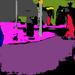
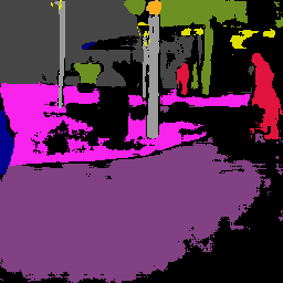
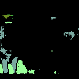
Semantic image synthesis/ generative models. Semantic image synthesis has played an important role in generative image compression from the very beginning [3, 56]. While its use has been primarily advertised for constrained application domains with semantic label maps available (e.g. the Cityscapes dataset  [11]), recent work  [40, 48, 4] as well as better semantic segmentation models [50, 10, 9, 58], show its generation ability across the image domain. Of particular importance to us is OASIS [48], a semantic image synthesis method based on pure adversarial supervision. In [48], the discriminator is repurposed to a ($N{+1}$)-class semantic segmentation network, where the additional class corresponds to the fake label in the original objective [17].

Other promising candidates we consider in this work are the SESAME [39], the U-Net [47] and the projected discriminators [46]. The SESAME discriminator has been introduced as a multi-scale and improved variant of the PatchGAN discriminator, while the use of U-Net and projected discriminators have led to significant advances over BigGAN [8] and StyleGAN  [28], respectively, arguably the two most popular GAN families.

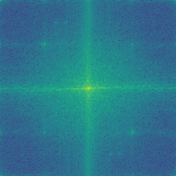
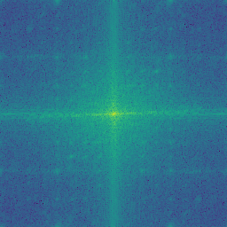
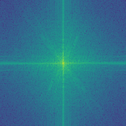
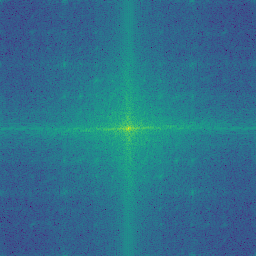
Another interesting line of work are frequency-aware GANs [26, 49, 15]. These methods are based on the observation that the statistics of GAN-generated images often differ significantly from real images in the frequency domain. In this work, we use the Focal Frequency Loss (FFL) [26] as a tool to quantify the frequency awareness of each method.

3 Background

Traditional rate-distortion trade-off. We follow the same notation as in previous works [34]: a neural image compression method typically consists of three components, an encoder $E$, a decoder $G$ (hereafter referred to as generator) and an entropy model $P$. Specifically, $E$ encodes $x$ to a quantized latent representation $y=E(x)$, while $G$ creates a reconstruction of the original image $x^{\prime}=G(y)$. The learning objective is to minimize the rate-distortion trade-off [12], with $\lambda>0$:

$$\mathcal{L}_{EGP}=\mathop{\mathbb{E}_{x\sim p_{X}}}[\lambda r(y)+d(x,x^{\prime})].$$ (1)

In Eq. 1, the bit-rate is estimated using the cross entropy $r(y)=-\log{P(y)}$, where $P(y)$ represents a probability model of $y$ and $d(x,x^{\prime})$ is a pairwise metric,  e.g. MSE. In practice, an entropy coding method based on $P$ is used to obtain the final bit representation, e.g. using adaptive arithmetic coding. For a more general overview of neural compression, we refer the interested reader to [62].

Rate-distortion-perception trade-off. In Mentzer et al. [34], the non-saturating loss [17] is further added to navigate the triple trade-off [7]:

$$\mathcal{L}_{EGP}=\mathop{\mathbb{E}_{x\sim p_{X}}}[\lambda r(y)+d(x,x^{\prime})-\beta\log(D(x^{\prime},y))],$$ (2)

$$\mathcal{L}_{D}={} \mathop{\mathbb{E}_{x\sim p_{X}}}[-\log(1-D(x^{\prime},y))]+$$ (3)

$$\mathop{\mathbb{E}_{x\sim p_{X}}}[-\log(D(x,y))].$$

In eq. (2), $d(x,x^{\prime})$ is decomposed into $d=k_{M}$MSE + $k_{P}$LPIPS [65], where $d_{M}$ and $d_{P}$ are hyper-parameters. We keep this formulation in our work to make use of the same hyper-parameters as in HiFiC. It is worth noting that the discriminator $D$ is conditioned on $y$, identical to the formulation under the ”optimal training framework”  [59]. Note that in both lines of work, a concatenation-based conditioning scheme [35] is chosen to model $P_{X|Y}$. We will study this design decision later on.

4 Our approach

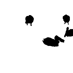
Learning objective. Inspired by recent advances in the field of semantic image synthesis [48], we redesign the discriminator to a ($N{+1}$)-class semantic segmentation task:

$$\mathcal{L}_{EGP}=\mathop{\mathbb{E}_{x\sim p_{X}}}[\lambda r(y)+d(x,x^{\prime})+\beta\mathcal{L}_{seg}(x^{\prime},y)],$$ (4)

$$\mathcal{L}_{D}={} \mathop{\mathbb{E}_{x\sim p_{X}}}[\mathcal{L}_{seg}(x,y)]+$$ (5)

$$\mathop{\mathbb{E}_{x\sim p_{X}}}[-\sum_{i,j}^{H\times W}\log D(x^{\prime},y)_{i,j,c_{ij}=N{+1}}].$$

In our formulation, $D\in\mathbb{R}^{H\times W\times N{+1}}$ represents a probability distribution over all semantic classes $\{1,..,N{+1}\}$, with $N{+1}$ being the fake label. Note that $D$ is conditioned on $y$ following theoretical and empirical results in [34, 59]. $\mathcal{L}_{seg}(x,y)=-\sum_{i,j}^{H\times W}w_{ij}\log D(x,y)_{i,j,c_{ij}}$ denotes the weighted ($N{+1}$)-class cross entropy loss over all pixel locations $(i,j)\in H\times W$, where $c_{ij}$ is the index of the prediction for the correct semantic class and $w_{ij}$ is a pixel weighting scheme. Different from the approach in [48], however, we employ the more commonly used pixel loss weighting scheme presented in [61], which puts more emphasis on small instances ($w_{ij}=3$ for area size smaller than $64\times 64$ px, $w_{ij}=1$ everywhere else). This change is primarily due to practical considerations which will be motivated later on.

Similar to the non-saturating loss, $G$ tries to fool $D$ by generating realistic and semantically correct reconstructions, whereas $D$ tries to differentiate between $x$ and $x^{\prime}$. This is essentially achieved by assigning the fake label as correct semantic class ($c_{ij}=N{+1}$). The discriminator is further regularized by the LabelMix consistency loss [48], which has been omitted in Eq. 5 for the sake of brevity. We provide additional details in the supplementary material.

Our approach shares some similarities with the VQ-VAE-based discriminator [55, 42] presented in MS-ILLM [38], with the main difference being the labels. In this work we directly employ human-annotated semantic labels, whereas Muckley et al. propose to replace these with codebook indices from a pre-trained VQ-VAE model. Our work is motivated by recent findings that pixel-level supervision of the discriminator is crucial in obtaining artifact-free images [49]. Codebook entries of VQ-VAEs on the other hand refer to patch-based supervision ($32\times 32$); the codebook size also typically exceeds the number of semantic labels ($1024$). Both approaches don’t require labels during inference and can thus be considered as an enhanced version of the GC ($D^{+}$)-variant introduced in [3].

Training strategies. Following HiFiC, we employ a two-stage training strategy. In the first stage, we use Eq. 4 without adversarial supervision (i.e. $\mathcal{L}_{EGP}=\mathop{\mathbb{E}_{x\sim p_{X}}}[\lambda r(y)+d(x,x^{\prime})]$), using the same configuration as in the original work [34]. For the second stage, we consider two variants: strategy-I denotes the full learning objective as described in Eq. 4 and  Eq. 5, whereas strategy-II is based on pure adversarial supervision inspired by [59]. In both cases, we only fine-tune $G$ and fix the pre-trained $E,P$ from stage one. The latter is motivated by the observation that an encoder trained under the traditional rate-distortion optimization is also well-suited for the perceptual compression task [59]. The outputs of our training procedure are shared weights for $E$, $P$, $G_{1}$ and $G_{2}$, from stages one and two, respectively.

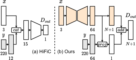
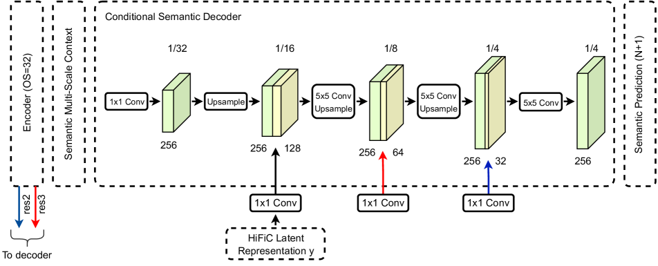
Model overview. We use the same backbones as in HiFiC [34, Fig. 2]/ SwinT-ChARM [66, Fig. 2] and thus focus mainly on the discriminator design in this section (Fig. 3). In HiFiC $y$ is pre-processed by a $3\times 3$ Convolution-SpectralNorm-LeakyReLU layer with $12$ filters and stride $1$, upsampled and concatenated with $x$ and subsequently fed into a PatchGAN discriminator [24]. In our work, we integrate an improved version of the OASIS discriminator [48], based on three simple yet effective changes: i) we use the same latent pre-processing blocks as in the original work (highlighted gray) but instead employ a pixel-wise projection-based conditioning scheme. ii) We replace spectral norm with weight norm, which increases the overall model capacity. iii) We pre-train the discriminator using DeepLab2 to accelerate training (highlighted orange). Note that this is motivated by the fact that we also start from a pre-trained $E$, $G$, $P$ state (training stage two). Our formulation shares some characteristics with [46], which projects samples to a pre-trained feature space, prior to classification. While in  [46] the pre-trained feature space is fixed, we fine-tune the whole model to learn the conditional distribution $P_{X|Y}$. We justify all our design decisions in more detail in Sec. 5.

Output residual prediction (ORP). For SwinT-ChARM, we further consider a lightweight retrofit solution based on transfer learning to obtain any point on the D-P curve from a single model on the receiver side. For that, we propose to clone the last Swin-transformer block [32] of the pre-trained $G_{2}$, which we refer to as $G_{ORP}$. The learning objective is to (implicitly) predict the residual $R$ between a MSE-optimized and GAN-optimized decoder output:

$$x^{\prime}=G_{2}(x)+(1-\alpha)R,$$ (6)

$$\mathcal{L}_{ORP}=\mathop{\mathbb{E}_{x\sim p_{X}}}[MSE(x,x^{\prime})]$$ (7)

with $R=G_{ORP}(F)$, where $F$ are feature maps extracted from $G_{2}(x)$. During training $\alpha=0$, which constraints x’ to the traditional MSE-optimized decoder output. During inference, $\alpha\in[0,1]$ allows traversing any point on the D-P curve using an implicitly encoded variant of image interpolation [25, 63]. Note that for $\alpha=1.0$, we always get the regular GAN-based output ($R$ is canceled out), which in practice is more difficult to obtain.

Figure 3: Schematic comparison of the discriminators used in (a) HiFiC [34]/MRIC [1] and (b) our work.

5 Exploring GANs for compression

In this section, we provide a preliminary study to identify suitable discriminator architectures/ GAN formulations for the task of generative image compression. For that, we review a wide variety of recently proposed candidates, including the PatchGAN [24], SESAME [39], U-Net [47], projected [46] and OASIS [48] discriminators. Here, we employ the training strategy-II for most parts, motivated by the observation that a perceptual decoder can be trained using solely a GAN conditioned on an encoder optimized under the traditional rate-distortion objective [59]. Intuitively, a good candidate should be able to generate high-fidelity reconstructions based on pure adversarial supervision.

Setup. We base our experiments on the official code base of HiFiC [34] and DeepLab2 [57], a TensorFlow library for deep labeling. In particular, we leverage DeepLab2’s sophisticated pre-processing pipeline, pre-trained semantic segmentation models (”DeepLabV3+” [10]), and pre-implemented loss functions. We use the same encoder, decoder and entropy architecture as in HiFiC, and only change the discriminator/ GAN learning objective for a fair comparison. The latter is motivated by recent theoretical arguments that the critic is decisive in matching the distribution of the training data [46]. We use the official implementation for PatchGAN and translate the SESAME, U-Net, projected and OASIS discriminators carefully to TensorFlow, based on the official PyTorch implementations. All our experiments start from stage two, using the same pre-trained $E$, $G$ and $P$. As a baseline, we use the official training configuration from HiFiC, however with a fixed $E$ and $P$ to enable identical bit-rates across all experiments.

Datasets. We use the Coco2017 panoptic dataset [31] with 118.287 training data and 133 semantic classes for stage one and our main experiments. To evaluate the generalization ability across the image domain, we use the same benchmarks as in HiFiC: DIV2K [2], CLIC 2020 [53] and Kodak [29]. DIV2K and CLIC 2020 are both high-resolution image datasets, which contain 100 and 428 images, respectively (see [34, A.9]); Kodak contains 24 images and is widely used as an image compression benchmark. For our preliminary study, we additionally consider a down-sized version of Cityscapes [11], which contains 19 semantic classes, 2975 training and 500 validation images, respectively. The image resolution is set here to $512\times 1024\times 3$.

Training and evaluation. We use the same hyper-parameters as in HiFiC, except the learning rate, which we fix to $1\mathrm{e}{-5}$ for stage two. For strategy-II, we set $\beta=1$ to rebalance $G$ and $D$. We further reduce the number of optimization steps on Cityscapes from 1M to 150k, considering the reduced size and complexity. We use PSNR and the FID-score [21] as a measure for distortion and perception, following recent work [34, 1]. More specifically, we compute the patched FID-score ”short FID/256” [34, A.7] based on the ”clean-FID” implementation [41] for our preliminary experiments on HiFiC. For our main experiments we have switched to torch-fidelity [41] to ease comparison to DIRAC and MRIC, where a recalculation based on clean-FID is currently prevented due to missing data. As common in the literature, we pad all images and crop the resulting reconstructions.

5.1 Comparing GAN approaches

Fairly comparing discriminator architectures/ GAN formulations for generative image compression is difficult due to the large variety in model design, conditioning scheme and regularization terms. It is also important to note that these methods were primarily co-designed with their respective generator structures, while we consider them in isolation. We make no claim to the superiority of one method over another, but rather are interested in their general suitability for generative image compression.

Here, we consider the low bit range ”HiFiC-lo”, where the influence of generative models is arguably greatest. For each method, we use the best configuration following the original work, including regularization terms. For projected GANs, we use the ”efficientnet-lite4”-variant [51] as a pre-trained feature network, which we have found to produce the best results; for OASIS, we investigate an additional backbone ”DeeplabV3+” [10], a close to state-of-the-art semantic segmentation method. We retrain DeeplabV3+ using DeepLab2 with a slightly adjusted prediction head ($N+1$ classes). We start our experiments by applying the same HiFiC-based conditioning scheme in all model variants. Our results are summarized in Tab. 1 and Fig. 4.

Method	Discriminator	Conditioning	GAN objective	Distortion		Perception
				PSNR $\uparrow$	rel-PSNR	FID $\downarrow$	rel-FID
baseline	PatchGAN [24]	concat	non-saturating	32.71	-	10.62	-
config-a	PatchGAN	concat	non-saturating	24.32	-25.6%	112.29	+957.3%
config-b	SESAME [39]	concat	hinge	29.43	-10.0%	75.65	+612.3%
config-c	U-Net [47]	concat	non-saturating	29.46	-9.9%	87.02	+719.4%
config-d	Projected [46]	concat	hinge	29.64	-9.5%	50.66	+377.0%
config-e	OASIS [48]	concat	cross entropy ($N{+1}$)	30.03	-8.2%	16.50	+55.4%
config-f	DeepLabV3+ [10]	concat	cross entropy ($N{+1}$)	21.53	-34.2%	20.61	+94.1%
config-c	U-Net	projection	non-saturating	29.38	-10.2%	30.80	+190.0%
config-e	OASIS	projection	cross entropy ($N{+1}$)	29.79	-8.9%	13.54	+27.5%
config-e	OASIS	implicit	cross entropy ($N{+1}$)	29.90	-8.6%	15.30	+44.1%

Table 1: Comparing GAN approaches for generative image compression on Cityscapes validation (0.092bpp). We report the PSNR, FID/256-score as well as the relative change over the baseline method (rel-PSNR, rel-FID).

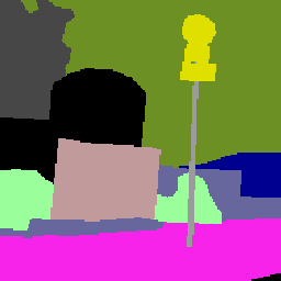
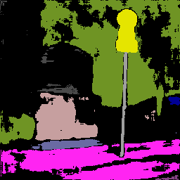
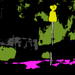
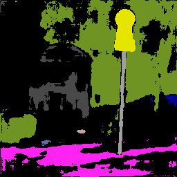
input	config-a/	config-b/	config-c/	config-d/	config-e/
	PatchGAN [24]	SESAME [39]	U-Net [47]	Projected [46]	OASIS [48]

Figure 4: Comparing various purely adversarially optimized generative image compression methods at low bit-rate ”HiFiC-lo”. Rows one and three show examples of reconstructed cropped images ($256\times 256$), while rows two and four show the corresponding spectra of the images. Best viewed electronically.

We make the following observations: unsurprisingly, no pure GAN-based configuration exceeds the performance of the baseline method ($32.71$dB PSNR, $10.62$ FID-score). The performance gaps range from $-34.2\%$ to $-8.2\%$ and $+957.3\%$ to $+94.1\%$ decrease in PSNR and FID-score, respectively. The PatchGAN discriminator performs worst, which is to be expected since it was designed primarily to penalize high-frequency structure in addition to the commonly used L1/L2 loss functions [24]. Indeed, when paired with an additional distortion loss, this formulation works remarkably well as demonstrated by the baseline configuration as well as by previous work [3, 25, 34, 1, 20].

We have found that both the SESAME, U-Net and projected discriminators produce similar strong PSNR values ($29.43-29.64$dB), with varying degrees of artifacts (see Fig. 4). The SESAME discriminator improves upon the PatchGAN variant due to its inherent multi-scale nature as well as access to additional semantic side information. For projected GANs we have found that the perceptual quality largely depends on the image resolution of the ”efficientnet-lite” feature extractors. We suppose that the (well hidden) gridding artifacts are due to a resolution mismatch; i.e. the efficientnet-lite variants are based on low resolutions images, e.g. $224\times 224$px for efficientnet-lite0, whereas HiFiC mostly targets high-resolution images up to $2000\times 2000$px.

The best purely adversarial method is achieved by OASIS, which significantly exceeds all its competitors in terms of perception (FID-score of $16.50$). We attribute its better performance to the semantically-aware pixel-level supervision, which implicitly provides a strong conditioning mechanism (see Tab. 1, config-e/ implicit conditioning). Note that a stronger semantic segmentation model does not per se lead to better performance (config-f). This finding is consistent with the observation that a stronger feature extractor does not necessarily lead to lower FID scores [46].

5.2 Investigating the conditioning scheme

We use the same setup as before, but now replace the vanilla concatenation-based conditioning scheme with projection [37] for some selected methods. For OASIS and U-Net, we employ a pixel-wise projection-based conditioning scheme; for U-Net we use an additional projection for the global output. We provide additional details in the supplementary material.

It can be observed that all projection-based configurations improve their base configurations while largely reducing image artifacts (see supplementary material). For optimization strategies with distortion, these considerations probably play a minor role, since $d$ already provides for a strong implicit conditioning mechanism. However, for approaches based on pure adversarial optimization, such as in the case of the ”optimal training framework” [59, 63], our findings shed some light on the lack of generalizability beyond the MNIST dataset.

5.3 Improving OASIS

Method	PSNR $\uparrow$	FID $\downarrow$
baseline	32.71	10.62
OASIS [48]	29.90	15.30
+ pre-trained	30.01	9.75
+ weight norm [44]	30.20	7.96
+ projection [37] (ours w/ o $d$)	29.97	7.74
ours w/ $d$	32.24	6.36

Table 2: Improving OASIS [48] step-by-step.

A major concern we had prior to the adoption was the tremendous amount of hardware resources required for training OASIS. Specifically, Schönfeld et al. trained their model on COCO-stuff for 4 weeks, in a multi-GPU environment ($4\times$ Tesla V100 GPUs). Instead, we target a single-GPU setup (Quadro RTX 6000, 24GB VRAM).

We attribute the slow training process to the spectral norm in its default configuration, which we have found to severely hinder learning progress. We note that similar observations have been reported recently, e.g. Lee et al. [30] proposed to multiply the normalized weight matrix with the spectral norm at initialization, which increases the often untuned Lipschitz constant and hence the overall model capacity. For our specific use case, we have found that weight normalization [44] combined with a pre-trained discriminator produces a good training speed/ stability/ compression performance trade-off (Tab. 2). In the supplementary material we further show that simply replacing the HiFiC discrimiantor with OASIS alone is not sufficient to improve over the state-of-the-art. This is especially true for highly complex learning tasks (Coco2017), where OASIS exhibits sever training instabilities.

6 Comparison to the state-of-the-art

Figure 5: Comparison to the state-of-the-art on CLIC 2020.

To compare to the state-of-the-art, we use the same setup as in  Sec. 5, except that we employ the training strategy-I, i.e. the GAN objective with distortion ”Ours w/ $d$”. For our main experiments, we consider SwinT-ChARM as backbone architecture; exact model configurations as well as extended experiments on HiFiC are summarized in the supplementary material.

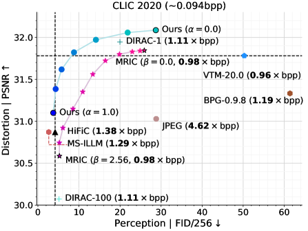
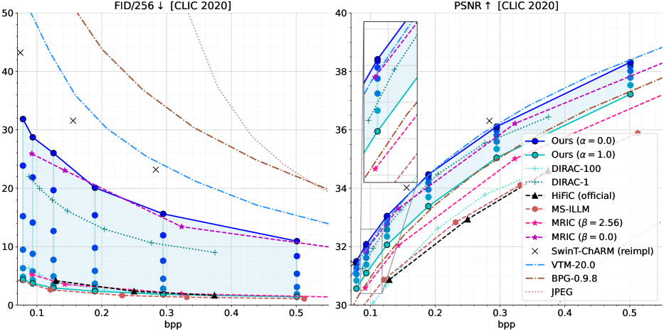
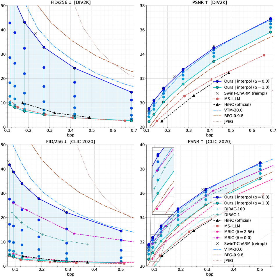
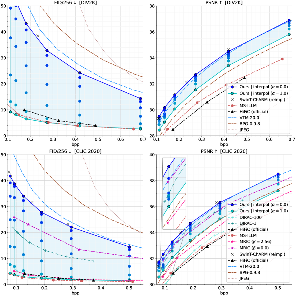
Baselines. We consider a wide-variety of baselines, including HiFiC [34], MS-ILLM [38], DIRAC-100 [16] and MRIC ($\beta=2.56$) [1] which correspond to the perception-oriented baselines, i.e. Ours ($\alpha=1.0$). Similarly, we consider VTM-20.0 (current state-of-the-art for non-learned image codecs), BPG-0.9.8, JPEG, DIRAC-1 [16] and MRIC ($\beta=0.0$) [1], which correspond to the distortion-oriented baselines, i.e. Ours ($\alpha=0.0$). Additionally, we add SwinT-ChARM (reimpl), our TensorFlow-reimplementation of SwinT-ChARM [66], which can be considered an upper bound for distortion.

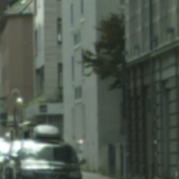
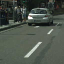
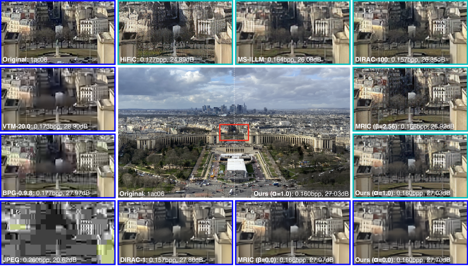
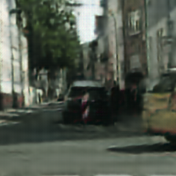
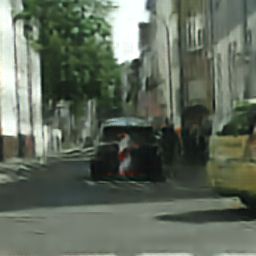
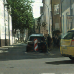
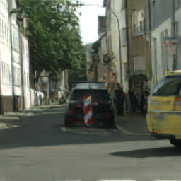
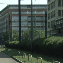
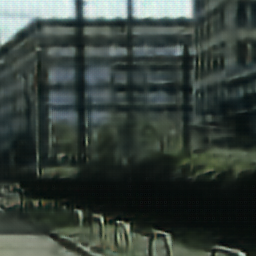
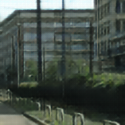
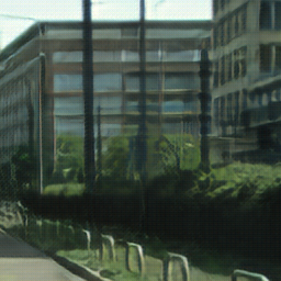
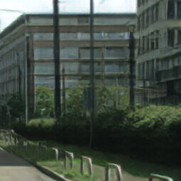
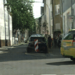
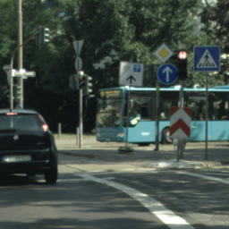
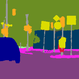
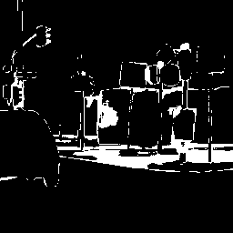
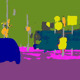
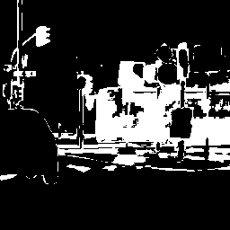
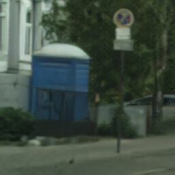
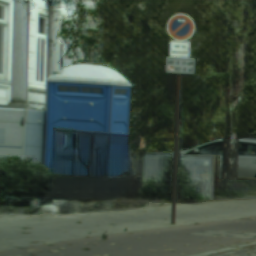
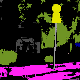
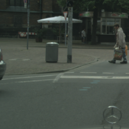
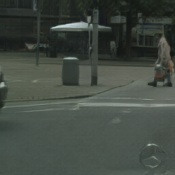
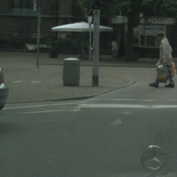
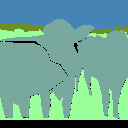
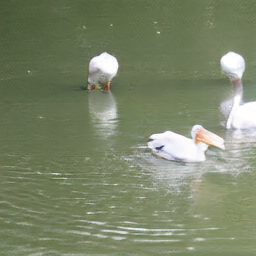
Objective and subjective comparisons on CLIC 2020 are summarized in Figure 5 and Fig. 2, respectively. We observe that Ours ($\alpha=1.0$) is most effective in the low to medium bit range, outperforming a wide variety of strong baselines in terms of distortion and perception, including HiFiC, MRIC ($\beta=2.56$) and DIRAC-100. Noteworthy, EGIC outperforms HiFiC-lo, the long standing previous state-of-the-art, even when using $30$% fewer bits. As we approach the extreme bit range ($<0.1$bpp), the performance differences grow up to $1.5$ FID points. Compared to MS-ILLM, we get slightly worse FID-scores, while having significantly better PSNR values.

For Ours ($\alpha=0.0$), we find that our proposed ORP is surprisingly strong, despite using a very lightweight design. For example, we require only $0.15\times$ of the additional model parameters introduced by the Fourier conditioning in MRIC [1], revealing that more sophisticated methods may in fact be unnecessary. In terms of distortion, our method outperforms MRIC and DIRAC, while (almost) matching VTM-20.0, the state-of-the-art for non-learned codecs. We further find that our method provides smooth D-P interpolation characteristics (Fig. 1), which makes it a promising candidate for practical applications.

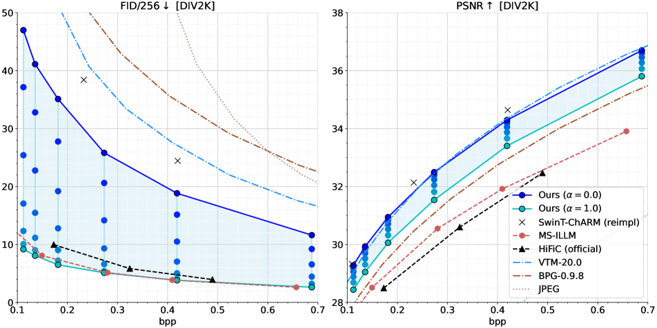
In the supplementary material we further provide a comprehensive comparison on DIV2K. Essentially, we get the same picture, except that our method outperforms MS-ILLM in the low bit range.

Finally, it is worth mentioning that EGIC is significantly more storage-efficient compared to all other methods. EGIC only requires a fraction of the number of model parameters compared to HiFiC/ MS-ILLM ($0.18\times$), DIRAC ($0.24\times$) and MRIC ($0.55\times$); in contrast to DIRAC, EGIC also only requires a single inference cycle.

7 Conclusion

We have developed EGIC, a novel generative image compression method that allows traversing the distortion-perception (D-P) curve efficiently from a single model on the receiver side. We find that EGIC is highly competitive, outperforming a wide variety of strong baselines (HiFiC, MRIC, DIRAC), while operating almost on par with VTM-20.0 on the distortion-oriented end of the spectrum. EGIC enjoys a simple and lightweight design with excellent interpolation characteristics, which makes it a promising candidate for practical applications targeting the low bit range.

Our code will be made publicly available upon publication to facilitate further research.

Appendix A Supplementary Material - EGIC

A.1 Detailed discriminator architecture

We summarize our discriminator architecture in Tab. 8. Our architecture is split into two parts. The first part (id=$1$) is identical to Schönfeld et al. (2021), except that we replace spectral norm with weight norm. The output ”out” is a $256\times 256\times{N+1}$ prediction map. In the second part (id=2), we adopt a pixel-wise projection-based conditioning scheme. We use a similar latent pre-processing block as in HiFiC, but use $64$ instead of $12$ filters. The pre-processed latent feature map ”latent_prep” has an identical shape as out and is subsequently incorporated into the discriminator, using projection (element-wise multiplication and sum across the channel dimension). The projected feature map proj is finally replicated and added back to out.

A.2 Pre-trained semantic segmentation models

Our discriminator block (id=$1$) is pre-trained using DeepLab2. We greatly rely on the panoptic configurations presented in https://github.com/google-research/deeplab2/blob/main/g3doc/projects/panoptic_deeplab.md. For all our experiments we use the ”ResNet-50” configuration as a starting point. We summarize the resulting performance of the pre-trained models in Tab. 3.

Dataset	Image crop	BS	Steps	mIoU $\uparrow$
Cityscapes	256	16	320k	0.67
Coco2017	256	16	1M	0.41

Table 3: Pre-trained discriminator performance measured by the mean intersection over union (mIoU). BS=batch size.

A.3 Additional experimental details

Preliminary study. To maintain the advantages of having pre-trained feature extractors, we use a slightly different concatenation-based conditioning scheme for config-f, see Fig. 9. Similar applies to config-d; we pre-process and concatenate the latent features with the efficientnet-lite4-based feature maps at each scale separately.

For config-c (projection), we use two separate latent pre-processing blocks with channel dimensions $64$ and $4$, corresponding to the local and global outputs, respectively. We use no resize operation for the latter to match the feature dimension prior to classification ($16*16*4=1024$).

Ours (SwinT-ChARM). We train six models ($\lambda\in\{2,1.5,1,0.5,0.25,0.1\}$) for 2+1M optimization steps, using a crop size of $256$ and a batch size of $16$ and $8$ for stage one and two, respectively. We use the Adam optimizer with default settings ($\beta_{1}=0.9,\beta_{2}=0.999$). For stage one, we use a learning rate of $1\mathrm{e}{-4}$ for the first $1.8$M steps and subsequently decay the learning rate to $1\mathrm{e}{-5}$, similar to previous work. For stage two, we use the same settings as in Ours w/ $d$ (HiFiC), i.e. training strategy-I with a fixed learning rate of $1\mathrm{e}{-5}$. ORP. We finetune $G_{ORP}$ for additional 2M steps. In practice we have found it slightly more efficient to directly predict the MSE-optimized decoder output $MSE_{pred}$ and to calculate $R=MSE_{pred}-G_{2}(x)$.

A.4 Comparing normalization strategies

We summarize some of the normalization methods we tried for OASIS in Tab. 4 and Fig. 15. For spectral norm, we have found that tuning the Lipschitz constant is indeed helpful. However, we did not find a configuration that exceeded the performance of the weight norm and hence omit it here. For layer norm we had to reduce the batch size to $8$, due to out-of-memory issues.

Method	mIoU $\uparrow$	PSNR $\uparrow$	FID $\downarrow$	BS
Spectral norm	0.49	30.01	9.75	16
Weight norm	0.67	30.20	7.96	16
Layer norm	0.68	29.49	9.00	8

Table 4: The effect of different normalization strategies on the semantic segmentation and its resulting compression performance.

A.5 LabelMix regularization

We additionally regularize the discriminator in Eq. 5 with the ”LabelMix” consistency loss introduced in (Schönfeld et al., 2021).

$$\mathcal{L}_{cons}={} \|D_{\text{logits}}(\text{LabelMix}(x,x^{\prime},M),y)-$$ (8)

$$\text{LabelMix}(D_{\text{logits}}(x,y),D_{\text{logits}}(x^{\prime},y),M)\|_{2}^{2},$$

with LabelMix($x,x^{\prime},M)=M\odot x+(1-M)\odot x^{\prime}$.

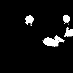
In Eq. 8, $M$ is a randomly generated binary mask that respects the underlying semantic boundaries of $x$ and LabelMix($x,x^{\prime},M$) corresponds to the resulting mixed real-fake image (in our case: real-reconstruction image). The discriminator predictions are constrained to be equivariant under the LabelMix operation, or in simple words, the discriminator prediction of the mixed image ($D_{\text{logits}}(\text{LabelMix}(x,x^{\prime},M),y)$) should be identical to the mixed discriminator predictions of the real and fake images, respectively ($\text{LabelMix}(D_{\text{logits}}(x,y),D_{\text{logits}}(x^{\prime},y),M)$), thus forcing the discriminator to focus more on content and structure. This is essentially achieved by applying the L2 norm on the unnormalized discriminator predictions $D_{\text{logits}}$. We used a fixed LabelMix coefficient of $10$ for all experiments.

We provide additional intuition for the LabelMix regularization term in Fig. 16 and Fig. 17, but refer the interested reader to the original paper for more details.

A.6 Performance on DIV2K

In Fig. 6, we provide an extended comparison to the state-of-the-art on DIV2K. We observe similar trends as discussed for CLIC 2020, except that our method matches/ even slightly outperforms MS-ILLM in terms of FID-score in the low bit range, while providing significantly better PSNR values.

Figure 6: Comparison to the state-of-the-art on DIV2K.

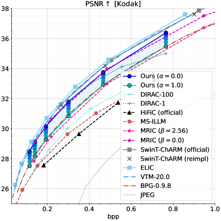
A.7 Performance on Kodak

In Fig. 7 we provide the rate-distortion performance for the Kodak dataset. We add the official values of SwinT-ChARM (Zhu et al., 2022) and ELIC (He et al., 2022) for reference. Exact configurations for JPEG, BPG-0.9.8 and VTM-20.0 can be found in Secs. A.16 to A.18.

Note that SwinT-ChARM is almost on par with the current state-of-the-art method ”ELIC” in terms of PSNR and thus represents a good base model for our work. The marginal gap is due to ELIC’s more powerful entropy model. We emphasize that both EGIC, MRIC and DIRAC rely on some variant of the ChARM-entropy model (Minnen et al., 2020).

Similar to MRIC, we observe that introducing higher perception results in a $1-1.5$dB PSNR decrease.

Figure 7: Kodak rate-distortion plot.

A.8 SwinT-ChARM reimplementation

In Fig. 7 we compare the compression performance of our SwinT-ChARM reimplementation (reimpl) to the official values, measured on the Kodak dataset. We optimized the reimplemented version for $2$M optimization steps on the CLIC 2020 training set, using $\lambda\in\{0.01,0.003,0.001,0.0003\}$ and a batch size of $8$. We used a learning rate of $1\mathrm{e}{-4}$ for the first $1.8$M steps and subsequently decayed the learning rate to $1\mathrm{e}{-5}$. We find that our reimplementation closely matches the official values (up to $0.1$dB tolerance), despite being trained from scratch and using less than two-thirds of the optimization steps.

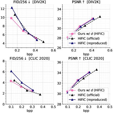
A.9 Experiments on HiFiC

In Fig. 8, we compare Ours w/ $d$ (HiFiC) to HiFiC (reproduced). Note that HiFiC (official) was trained on an internal dataset is therefore only visualized for transparency reasons. We observe that Ours w/ $d$ (HiFiC) is most effective in the low to medium bit range, which is the key focus of our work. For HiFiC-lo, we achieve an improvement of up to 2 FID points with slightly better PSNR (+0.2dB), suggesting that our method is particularly well suited for the extremely low bit range $<0.1$bpp.

For HiFiC-hi, we experience a slight decrease in performance. We suspect that this is due to misaligned hyper-parameters; indeed recent work suggests that a separate set of hyper-parameters is required for various bit-rates (Muckley et al., 2023).

Figure 8: Relative comparison to HiFiC.

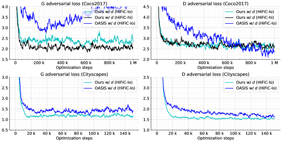
A.10 Comparing training dynamics

In Fig. 10 we compare the training dynamics of OASIS w/ $d$ and Ours w/ $d$. We find that OASIS with weight norm greatly increases model capacity, while pre-training accelerates training, resulting in superior compression performance. Note that our method provides robust and stable training across different compression rates, while OASIS w/ $d$ exhibits training instabilities that are particularly evident on complex datasets (Coco2017).

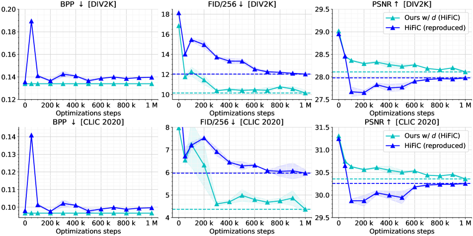
In Fig. 11 we provide further performance insights into the training dynamics of Ours w/ $d$ (HiFiC) and HiFiC (reproduced) for stage two. We report the means and standard deviations of BPP, PSNR, and FID as a function of the number of optimization steps across two test runs. Note that HiFiC’s training procedure is divided into 3 phases: warm-up ($0-50$k), training with a learning rate of $1\mathrm{e}{-4}$ ($50-500$k) and $1\mathrm{e}{-5}$ ($500$k-$1$M), respectively, whereas, Ours w/ $d$ (HiFiC) uses the same learning rate and $\lambda$-schedule across all training steps.

We find that our method significantly accelerates training progress, similar to projected GANs (Sauer et al., 2021). As can be seen, our method exceeds the performance of HiFiC after only $300$k optimization steps. The large deviations at the beginning of the training phase can be attributed to a sort of calibration phase in which the variables for the projection-based conditioning mechanism are learned from scratch.

A.11 Impact of the focal frequency loss

In Tab. 5, we summarize the effect of the focal frequency loss (FFL) introduced in Jiang et al. (2021) on the concat base configurations. For that, we finetune all base models for additional 50k steps. We find that the FFL has the greatest impact on config-a and config-d, whereas it has little impact on the discriminators based on pixel-level supervision (config-c and config-e). We also find that the FFL cannot further improve ours w/ o $d$, which reinforces the design decisions made in our work.

Method	Distortion		Perception
+FFL	PSNR $\uparrow$	rel-PSNR	FID $\downarrow$	rel-FID
config-a	32.53	+33.8%	40.64	-63.8%
config-b	29.17	-0.9%	79.55	+5.2%
config-c	29.23	-0.8%	89.73	+3.1%
config-d	29.89	+1.7%	21.85	-29.1%
config-e	30.25	+0.7%	15.93	-3.5%
ours w/o $d$	29.56	-1.4%	8.73	+12.8%

Table 5: Which method benefits the most from the FFL? The relative change (rel-PSNR, rel-FID) is here denoted over their respective concat-base configurations.

A.12 Model size comparison

In Tab. 6, we compare the storage-efficiency of each model in terms of model parameters (in millions). For the generator, we further differentiate between the base model size and additional parameters required for traversing the D-P curve (denoted by $+$). The calculation for $P$ includes the hyper-analysis and hyper-synthesis transforms, as well as additional slice transforms in the case of ChARM.

Method	$E$	$G$	$P$	Total (M)
HiFiC (Mentzer et al., 2020)	7.4	156.8	17.3	181.5
MS-ILLM (Muckley et al., 2023)	7.4	156.8	17.3	181.5
DIRAC (Hoogeboom et al., 2023)	7.0	7.0 + 108.4	14.3	136.8
MRIC (Agustsson et al., 2023)	10.7	10.7 + 2.65	36.4	60.45
EGIC (Ours)	9.1	9.1 + 0.4	14.4	33

Table 6: Model size comparison in millions of parameters (M).

A.13 Image/ weight interpolation

EGIC also allows targeting different points on the D-P curve using image/ weight interpolation (Wang et al. 2019, Iwai et al. 2021, Yan et al. 2022), thanks to our two-stage training procedure. For that, we fine-tune the generator weights from stage one $G_{1}$ for additional 500k optimization steps using only MSE as distortion loss to match Ours ($\alpha=0.0$). Image and weight interpolation can be achieved using

$$x^{\prime}=(1-\alpha)G_{1}(y)+\alpha G_{2}(y)$$ (9)

and

$$x^{\prime}=G_{\theta}(y);\theta=(1-\alpha)\theta_{G_{1}}+\alpha\theta_{G_{2}},$$ (10)

respectively, where $\theta$ are the parameters of $G$ and $\alpha$ is the interpolation weight. We use $\alpha\in\{0.0,0.17,0.33,0.5,0.67,0.83,1.0\}$, resulting in seven points per bit-rate.

Our results are summarized in Fig. 12 and Fig. 13. As can be seen, EGIC with image interpolation works quite well. We also find that weight interpolation works reasonably well, however with skewed interpolation characteristics in some cases (e.g. CLIC 2020 at low bit-rate). Noteworthy, Ours $|$ interpol ($\alpha=0.0$) almost matches the performance of SwinT-ChARM (reimpl), which can be considered an upper bound. While these methods are known to provide strong results, they are not well suited from a practical perspective, due to extensive additional compute and/or storage requirements.

A.14 Visual comparison: concat vs. projection

In Fig. 14 we provide additional visual impressions of the effect of various conditioning strategies. We find that projection greatly helps to reduce image artifacts.

A.15 Pixel weighting schemes

Pixel weighting schemes have played a minor role in our work. As mentioned earlier, we use the simple instance size-based weighting scheme introduced in Yang et al. (2019), whereas, in Schönfeld et al. (2021), each semantic class is weighted by its inverse per-pixel frequency, computed over a batch of images. In Tab. 7 we show that this method is indeed effective and performs comparably to the more sophisticated approach of Schönfeld et al. (2021). In Fig. 18 we provide additional visual comparisons.

Method	PSNR $\uparrow$	FID $\downarrow$
OASIS (instance size-oriented)	29.90	15.30
OASIS (class-oriented)	29.90	15.56

Table 7: Comparing different pixel weighting schemes.

A.16 Comparison to VVC-intra

The evaluation of the VVC standard (current state-of-the-art for non-learned image compression codecs) is based on VTM-20.0, a reference software provided by https://vcgit.hhi.fraunhofer.de/jvet/VVCSoftware_VTM/-/releases/VTM-20.0. Similar to previous work, we first convert the PNG images to YCbCr-format using ffmpeg https://www.ffmpeg.org/:

ffmpeg
-i $PNGPATH -pix_fmt yuv444p $YUVPATH

To compress/ decompress the images, we use:

# Encode
EncoderAppStatic
-c encoder_intra_vtm.cfg
-i $YUVPATH -q $Q, -o /dev/null
-b $OUTPUT
--SourceWidth=$WIDTH
--SourceHeight=$HEIGHT
--FrameRate=1 --FramesToBeEncoded=1
--InputBitDepth=8
--InputChromaFormat=444
--ConformanceWindowMode=1

# Decode
DecoderAppStatic
-b $OUTPUT -o $RECON -d 8

To convert the outputs back to PNG-format, we use:

ffmpeg
-f rawvideo -s $WIDTHx$HEIGHT
-pix_fmt yuv444p -i $RECON $RECON_PNG

PSNR is measured on the 8bit-decoded images and not on the floating point reconstructions, which is consistent with all our comparisons.

A.17 Comparison to BPG

The evaluation of BPG-0.9.8 is based on the HEVC open video compression standard, provided by https://bellard.org/bpg/.

We use the following commands:

# Encode
bpgenc -o $OUTPUT -q $Q
-f 444 -e x265 -b 8 $INPUT

# Decode
bpgdec -o $RECON $OUTPUT

A.18 Comparison to JPEG

We use the Python Imaging Library (PIL) to obtain the JPEG encoded/ decoded images:

tmp = io.BytesIO()
img.save(tmp, format=’jpeg’,
         subsampling=0,
         quality=Q)
tmp.seek(0)
filesize = tmp.getbuffer().nbytes
bpp = filesize * float(8)/
      img.size[0] * img.size[1]
rec = Image.open(tmp)

We set (chroma) subsampling to $0$, which corresponds to $4:4:4$, the highest quality settings.

Id	Operation	Input	Size	Output	Size
	ResBlock-Down	image (x)	$256\times 256\times 3$	down_1	$128\times 128\times 128$
	ResBlock-Down	down_1	$128\times 128\times 128$	down_2	$64\times 64\times 128$
	ResBlock-Down	down_2	$64\times 64\times 128$	down_3	$32\times 32\times 256$
	ResBlock-Down	down_3	$32\times 32\times 256$	down_4	$16\times 16\times 256$
	ResBlock-Down	down_4	$16\times 16\times 256$	down_5	$8\times 8\times 512$
	ResBlock-Down	down_5	$8\times 8\times 512$	down_6	$4\times 4\times 512$
1	ResBlock-Up	down_6	$4\times 4\times 512$	up_1	$8\times 8\times 512$
	ResBlock-Up	cat(up_1, down_5)	$8\times 8\times 1024$	up_2	$16\times 16\times 256$
	ResBlock-Up	cat(up_2, down_4)	$16\times 16\times 512$	up_3	$32\times 32\times 256$
	ResBlock-Up	cat(up_3, down_3)	$32\times 32\times 512$	up_4	$64\times 64\times 128$
	ResBlock-Up	cat(up_4, down_2)	$64\times 64\times 256$	up_5	$128\times 128\times 128$
	ResBlock-Up	cat(up_5, down_1)	$128\times 128\times 256$	up_6	$256\times 256\times 64$
	Conv2D	up_6	$256\times 256\times 64$	out	$256\times 256\times{N+1}$
	Conv2D + Resize	latent (y)	$16\times 16\times{C_{y}}$	latent_prep	$256\times 256\times 64$
2	Projection	(up_6, latent_prep)	$256\times 256\times 64$	proj	$256\times 256\times 1$
	Add	(out, proj)	$256\times 256\times{N+1}$	D_out	$256\times 256\times{N+1}$

Table 8: The OASIS-based discriminator used in our main experiments. ${C_{y}}\in\{220,320\}$.

Figure 9: Conditional panoptic DeepLab-based semantic decoder (config-f). We seamlessly integrate $y$ using a similar HiFiC-based concatenation scheme. Note that this formulation allows to keep the benefits of pre-trained feature extractors (”resnet50”).

Figure 10: Comparing the training dynamics of OASIS w/ $d$ and Ours w/ $d$. ”G adversarial” corresponds to the ($N{+1}$)-cross entropy loss and hence gives an idea of how realistic and semantically correct the resulting reconstructions are (lower is better). ”D adversarial” includes regularization terms (lower is better).

Figure 11: BPP, FID, and PSNR vs. optimization steps for the second stage of Ours w/ $d$ (HiFiC) and HiFiC (reproduced). We show the mean and standard deviation across 2 runs per setting. Values at step $0$ correspond to the output values from stage one. We additionally show the values at step $50$k (warm-up phase in HiFiC).

Figure 12: Traversing the rate-distortion-perception plane using image interpolation.

Figure 13: Traversing the rate-distortion-perception plane using weight interpolation.

input	config-c/	config-c/
	concat	projection

Figure 14: U-Net: config-c/ concat vs. config-c/ projection. Note that projection significantly reduces image artifacts.

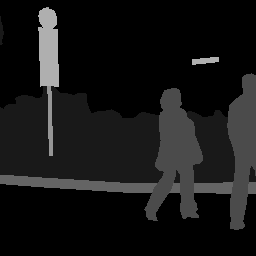
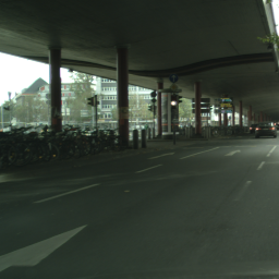
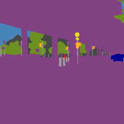
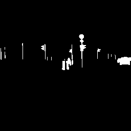
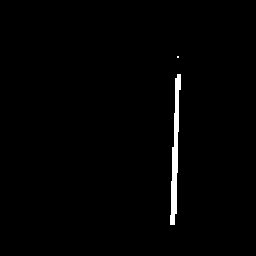
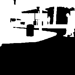
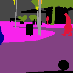
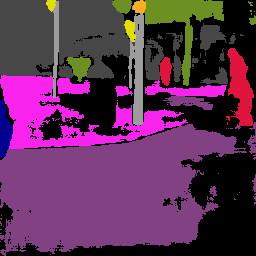
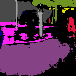
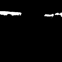
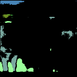
input	semantic prediction	error map
	OASIS with weight normalization
	OASIS with spectral normalization

Figure 15: Comparing the semantic segmentation performance between OASIS with weight normalization and OASIS with spectral normalization. Black pixels in the error map correspond to perfect prediction, white pixels highlight deviations from the ground truth.

input $x$	reconstruction $x^{\prime}$	$\text{LabelMix}_{(x,x^{\prime},M)}$	Mask $M$	pixel weights $w$
label map	${D_{(x,y)}}$	${D_{(x^{\prime},y)}}$	$D_{\text{(LM}{(x,x^{\prime},M),y)}}$	$\text{LM}_{(D(x,y),D(x^{\prime},y),M)}$
input $x$	reconstruction $x^{\prime}$	$\text{LabelMix}_{(x,x^{\prime},M)}$	Mask $M$	pixel weights $w$
label map	${D_{(x,y)}}$	${D_{(x^{\prime},y)}}$	$D_{\text{(LM}{(x,x^{\prime},M),y)}}$	$\text{LM}_{(D(x,y),D(x^{\prime},y),M)}$

Figure 16: Visualizing the discriminator loss components at step 33.5k (top row) and 35.2k (bottom row) on the Cityscapes dataset. We use an abbreviated notation in some cases due to space constraints; LM=LabelMix. $M$, $\text{LabelMix}_{(x,x^{\prime},M)}$, $D_{\text{(LM}{(x,x^{\prime},M),y)}}$ and $\text{LM}_{(D(x,y),D(x^{\prime},y),M)}$ correspond to the terms introduced in  Sec. A.5. We additionally visualize the pixel weight masks $w$ introduced in Sec. 4 that highlight small object instances, as well as the corresponding label maps and the discriminator predictions for $x$ and $x^{\prime}$, respectively. The colorized discriminator predictions are obtained by $\operatorname*{arg\,max}(D)$. The black color corresponds to the fake class.

input $x$	reconstruction $x^{\prime}$	$\text{LabelMix}_{(x,x^{\prime},M)}$	Mask $M$	pixel weights $w$
label map	${D_{(x,y)}}$	${D_{(x^{\prime},y)}}$	$D_{\text{(LM}{(x,x^{\prime},M),y)}}$	$\text{LM}_{(D(x,y),D(x^{\prime},y),M)}$
input $x$	reconstruction $x^{\prime}$	$\text{LabelMix}_{(x,x^{\prime},M)}$	Mask $M$	pixel weights $w$
label map	${D_{(x,y)}}$	${D_{(x^{\prime},y)}}$	$D_{\text{(LM}{(x,x^{\prime},M),y)}}$	$\text{LM}_{(D(x,y),D(x^{\prime},y),M)}$

Figure 17: Visualizing the discriminator loss components at step 1M (top row) and at an early training stage (160k, bottom row) on the Coco2017 dataset. See Fig. 16 for a detailed description.

input $x$	label map	pixel weights $w$	pixel weights $w$
		(Yang et al., 2019)	(Schönfeld et al., 2021)

Figure 18: Pixel weighting schemes based on instance size (third column) vs. class imbalance (fourth column). We map the pixel weights $w$ to a pre-defined color map for better visualization; the brighter the color, the larger the weight. Note that in Schönfeld et al. (2021) identical class segments share the same pixel weights (same color).

References

- [1] Eirikur Agustsson, David Minnen, George Toderici, and Fabian Mentzer. Multi-realism image compression with a conditional generator. In Proceedings of the IEEE/CVF Conference on Computer Vision and Pattern Recognition (CVPR), pages 22324–22333, June 2023.
- [2] Eirikur Agustsson and Radu Timofte. Ntire 2017 challenge on single image super-resolution: Dataset and study. In The IEEE Conference on Computer Vision and Pattern Recognition (CVPR) Workshops, 2017.
- [3] Eirikur Agustsson, Michael Tschannen, Fabian Mentzer, Radu Timofte, and Luc Van Gool. Generative adversarial networks for extreme learned image compression. In Proceedings of the IEEE International Conference on Computer Vision, 2019.
- [4] Dor Arad Hudson and Larry Zitnick. Compositional transformers for scene generation. In M. Ranzato, A. Beygelzimer, Y. Dauphin, P.S. Liang, and J. Wortman Vaughan, editors, Advances in Neural Information Processing Systems, volume 34, pages 9506–9520. Curran Associates, Inc., 2021.
- [5] Martin Arjovsky, Soumith Chintala, and Léon Bottou. Wasserstein generative adversarial networks. In Doina Precup and Yee Whye Teh, editors, Proceedings of the 34th International Conference on Machine Learning, volume 70 of Proceedings of Machine Learning Research, pages 214–223. PMLR, 06–11 Aug 2017.
- [6] Johannes Ballé, David Minnen, Saurabh Singh, Sung Jin Hwang, and Nick Johnston. Variational image compression with a scale hyperprior. In International Conference on Learning Representations, 2018.
- [7] Yochai Blau and Tomer Michaeli. Rethinking Lossy Compression: The Rate-Distortion-Perception Tradeoff. In Proceedings of the 36th International Conference on Machine Learning, 2019.
- [8] Andrew Brock, Jeff Donahue, and Karen Simonyan. Large scale GAN training for high fidelity natural image synthesis. In International Conference on Learning Representations, 2019.
- [9] Liang-Chieh Chen, Yukun Zhu, George Papandreou, Florian Schroff, and Hartwig Adam. Encoder-decoder with atrous separable convolution for semantic image segmentation. In ECCV, 2018.
- [10] Bowen Cheng, Maxwell D Collins, Yukun Zhu, Ting Liu, Thomas S Huang, Hartwig Adam, and Liang-Chieh Chen. Panoptic-deeplab: A simple, strong, and fast baseline for bottom-up panoptic segmentation. In CVPR, 2020.
- [11] Marius Cordts, Mohamed Omran, Sebastian Ramos, Timo Rehfeld, Markus Enzweiler, Rodrigo Benenson, Uwe Franke, Stefan Roth, and Bernt Schiele. The cityscapes dataset for semantic urban scene understanding. In Proc. of the IEEE Conference on Computer Vision and Pattern Recognition (CVPR), 2016.
- [12] Thomas M Cover and Joy A Thomas. Elements of information theory. John Wiley & Sons, 2012.
- [13] Prafulla Dhariwal and Alexander Nichol. Diffusion models beat gans on image synthesis. In M. Ranzato, A. Beygelzimer, Y. Dauphin, P.S. Liang, and J. Wortman Vaughan, editors, Advances in Neural Information Processing Systems, volume 34, pages 8780–8794. Curran Associates, Inc., 2021.
- [14] Alexey Dosovitskiy and Josip Djolonga. You only train once: Loss-conditional training of deep networks. In International Conference on Learning Representations, 2020.
- [15] Rinon Gal, Dana Cohen Hochberg, Amit Bermano, and Daniel Cohen-Or. Swagan: A style-based wavelet-driven generative model. ACM Trans. Graph., 40(4), July 2021.
- [16] Noor F. Ghouse, Jens Petersen, Auke Wiggers, Tianlin Xu, and Guillaume Sautière. A Residual Diffusion Model for High Perceptual Quality Codec Augmentation. arXiv: 2301.05489, 2023.
- [17] Ian Goodfellow, Jean Pouget-Abadie, Mehdi Mirza, Bing Xu, David Warde-Farley, Sherjil Ozair, Aaron Courville, and Yoshua Bengio. Generative adversarial nets. In Z. Ghahramani, M. Welling, C. Cortes, N. Lawrence, and K.Q. Weinberger, editors, Advances in Neural Information Processing Systems, volume 27. Curran Associates, Inc., 2014.
- [18] Ishaan Gulrajani, Faruk Ahmed, Martin Arjovsky, Vincent Dumoulin, and Aaron C Courville. Improved training of wasserstein gans. In I. Guyon, U. Von Luxburg, S. Bengio, H. Wallach, R. Fergus, S. Vishwanathan, and R. Garnett, editors, Advances in Neural Information Processing Systems, volume 30. Curran Associates, Inc., 2017.
- [19] Dailan He, Ziming Yang, Weikun Peng, Rui Ma, Hongwei Qin, and Yan Wang. Elic: Efficient learned image compression with unevenly grouped space-channel contextual adaptive coding. In Proceedings of the IEEE/CVF Conference on Computer Vision and Pattern Recognition (CVPR), pages 5718–5727, June 2022.
- [20] Dailan He, Ziming Yang, Hongjiu Yu, Tongda Xu, Jixiang Luo, Yuan Chen, Chenjian Gao, Xinjie Shi, Hongwei Qin, and Yan Wang. Po-elic: Perception-oriented efficient learned image coding. In Proceedings of the IEEE/CVF Conference on Computer Vision and Pattern Recognition (CVPR) Workshops, pages 1764–1769, June 2022.
- [21] Martin Heusel, Hubert Ramsauer, Thomas Unterthiner, Bernhard Nessler, and Sepp Hochreiter. Gans trained by a two time-scale update rule converge to a local nash equilibrium. In Advances in Neural Information Processing Systems, 2017.
- [22] Jonathan Ho, Ajay Jain, and Pieter Abbeel. Denoising diffusion probabilistic models. In H. Larochelle, M. Ranzato, R. Hadsell, M.F. Balcan, and H. Lin, editors, Advances in Neural Information Processing Systems, volume 33, pages 6840–6851. Curran Associates, Inc., 2020.
- [23] Emiel Hoogeboom, Eirikur Agustsson, Fabian Mentzer, Luca Versari, George Toderici, and Lucas Theis. High-Fidelity Image Compression with Score-based Generative Models. arXiv: 2305.18231, 2023.
- [24] Phillip Isola, Jun-Yan Zhu, Tinghui Zhou, and Alexei A Efros. Image-to-image translation with conditional adversarial networks. CVPR, 2017.
- [25] S. Iwai, T. Miyazaki, Y. Sugaya, and S. Omachi. Fidelity-controllable extreme image compression with generative adversarial networks. In 2020 25th International Conference on Pattern Recognition (ICPR), pages 8235–8242, Los Alamitos, CA, USA, jan 2021. IEEE Computer Society.
- [26] Liming Jiang, Bo Dai, Wayne Wu, and Chen Change Loy. Focal frequency loss for image reconstruction and synthesis. In ICCV, 2021.
- [27] Justin Johnson, Alexandre Alahi, and Li Fei-Fei. Perceptual losses for real-time style transfer and super-resolution. In Bastian Leibe, Jiri Matas, Nicu Sebe, and Max Welling, editors, Computer Vision – ECCV 2016, pages 694–711, Cham, 2016. Springer International Publishing.
- [28] Tero Karras, Miika Aittala, Janne Hellsten, Samuli Laine, Jaakko Lehtinen, and Timo Aila. Training generative adversarial networks with limited data. In H. Larochelle, M. Ranzato, R. Hadsell, M.F. Balcan, and H. Lin, editors, Advances in Neural Information Processing Systems, volume 33, pages 12104–12114. Curran Associates, Inc., 2020.
- [29] Eastman Kodak. Kodak lossless true color image suite (PhotoCD PCD0992).
- [30] Kwonjoon Lee, Huiwen Chang, Lu Jiang, Han Zhang, Zhuowen Tu, and Ce Liu. ViTGAN: Training GANs with vision transformers. In International Conference on Learning Representations, 2022.
- [31] Tsung-Yi Lin, Michael Maire, Serge J. Belongie, James Hays, Pietro Perona, Deva Ramanan, Piotr Dollár, and C. Lawrence Zitnick. Microsoft coco: Common objects in context. In ECCV, 2014.
- [32] Ze Liu, Yutong Lin, Yue Cao, Han Hu, Yixuan Wei, Zheng Zhang, Stephen Lin, and Baining Guo. Swin transformer: Hierarchical vision transformer using shifted windows. In Proceedings of the IEEE/CVF International Conference on Computer Vision (ICCV), 2021.
- [33] Xudong Mao, Qing Li, Haoran Xie, Raymond Y.K. Lau, Zhen Wang, and Stephen Paul Smolley. Least squares generative adversarial networks. In Proceedings of the IEEE International Conference on Computer Vision (ICCV), Oct 2017.
- [34] Fabian Mentzer, George D Toderici, Michael Tschannen, and Eirikur Agustsson. High-fidelity generative image compression. Advances in Neural Information Processing Systems, 2020.
- [35] Mehdi Mirza and Simon Osindero. Conditional generative adversarial nets. arXiv: 1411.1784, 2014.
- [36] Takeru Miyato, Toshiki Kataoka, Masanori Koyama, and Yuichi Yoshida. Spectral normalization for generative adversarial networks. In International Conference on Learning Representations, 2018.
- [37] Takeru Miyato and Masanori Koyama. cGANs with projection discriminator. In International Conference on Learning Representations, 2018.
- [38] Matthew J. Muckley, Alaaeldin El-Nouby, Karen Ullrich, Herve Jegou, and Jakob Verbeek. Improving statistical fidelity for neural image compression with implicit local likelihood models. In Andreas Krause, Emma Brunskill, Kyunghyun Cho, Barbara Engelhardt, Sivan Sabato, and Jonathan Scarlett, editors, Proceedings of the 40th International Conference on Machine Learning, volume 202 of Proceedings of Machine Learning Research, pages 25426–25443. PMLR, 23–29 Jul 2023.
- [39] Evangelos Ntavelis, Andrés Romero, Iason Kastanis, Luc Van Gool, and Radu Timofte. SESAME: Semantic Editing of Scenes by Adding, Manipulating or Erasing Objects. In Andrea Vedaldi, Horst Bischof, Thomas Brox, and Jan-Michael Frahm, editors, Computer Vision – ECCV 2020, pages 394–411, Cham, 2020. Springer International Publishing.
- [40] Taesung Park, Ming-Yu Liu, Ting-Chun Wang, and Jun-Yan Zhu. Semantic image synthesis with spatially-adaptive normalization. In Proceedings of the IEEE Conference on Computer Vision and Pattern Recognition, 2019.
- [41] Gaurav Parmar, Richard Zhang, and Jun-Yan Zhu. On aliased resizing and surprising subtleties in gan evaluation. In CVPR, 2022.
- [42] Ali Razavi, Aaron van den Oord, and Oriol Vinyals. Generating diverse high-fidelity images with vq-vae-2. In H. Wallach, H. Larochelle, A. Beygelzimer, F. d'Alché-Buc, E. Fox, and R. Garnett, editors, Advances in Neural Information Processing Systems, volume 32. Curran Associates, Inc., 2019.
- [43] Oren Rippel and Lubomir Bourdev. Real-time adaptive image compression. In Proceedings of the 34th International Conference on Machine Learning, 2017.
- [44] Tim Salimans and Durk P Kingma. Weight normalization: A simple reparameterization to accelerate training of deep neural networks. In D. Lee, M. Sugiyama, U. Luxburg, I. Guyon, and R. Garnett, editors, Advances in Neural Information Processing Systems, volume 29. Curran Associates, Inc., 2016.
- [45] Shibani Santurkar, David Budden, and Nir Shavit. Generative compression. In 2018 Picture Coding Symposium (PCS), pages 258–262, 2018.
- [46] Axel Sauer, Kashyap Chitta, Jens Müller, and Andreas Geiger. Projected gans converge faster. In Advances in Neural Information Processing Systems (NeurIPS), 2021.
- [47] Edgar Schonfeld, Bernt Schiele, and Anna Khoreva. A u-net based discriminator for generative adversarial networks. In Proceedings of the IEEE/CVF Conference on Computer Vision and Pattern Recognition, 2020.
- [48] Edgar Schönfeld, Vadim Sushko, Dan Zhang, Juergen Gall, Bernt Schiele, and Anna Khoreva. You only need adversarial supervision for semantic image synthesis. In International Conference on Learning Representations, 2021.
- [49] Katja Schwarz, Yiyi Liao, and Andreas Geiger. On the frequency bias of generative models. In M. Ranzato, A. Beygelzimer, Y. Dauphin, P.S. Liang, and J. Wortman Vaughan, editors, Advances in Neural Information Processing Systems, volume 34, pages 18126–18136. Curran Associates, Inc., 2021.
- [50] Nasim Souly, Concetto Spampinato, and Mubarak Shah. Semi supervised semantic segmentation using generative adversarial network. In 2017 IEEE International Conference on Computer Vision (ICCV), 2017.
- [51] Mingxing Tan and Quoc Le. EfficientNet: Rethinking model scaling for convolutional neural networks. In Kamalika Chaudhuri and Ruslan Salakhutdinov, editors, Proceedings of the 36th International Conference on Machine Learning, volume 97 of Proceedings of Machine Learning Research, pages 6105–6114. PMLR, 09–15 Jun 2019.
- [52] Lucas Theis, Tim Salimans, Matthew Douglas Hoffman, and Fabian Mentzer. Lossy compression with gaussian diffusion, 2023.
- [53] George Toderici, Lucas Theis, Nick Johnston, Eirikur Agustsson, Fabian Mentzer, Johannes Ballé, Wenzhe Shi, and Radu Timofte. Clic 2020: Challenge on learned image compression, 2020.
- [54] Michael Tschannen, Eirikur Agustsson, and Mario Lucic. Deep generative models for distribution-preserving lossy compression. In S. Bengio, H. Wallach, H. Larochelle, K. Grauman, N. Cesa-Bianchi, and R. Garnett, editors, Advances in Neural Information Processing Systems, volume 31. Curran Associates, Inc., 2018.
- [55] Aaron van den Oord, Oriol Vinyals, and koray kavukcuoglu. Neural discrete representation learning. In I. Guyon, U. Von Luxburg, S. Bengio, H. Wallach, R. Fergus, S. Vishwanathan, and R. Garnett, editors, Advances in Neural Information Processing Systems, volume 30. Curran Associates, Inc., 2017.
- [56] Ting-Chun Wang, Ming-Yu Liu, Jun-Yan Zhu, Andrew Tao, Jan Kautz, and Bryan Catanzaro. High-resolution image synthesis and semantic manipulation with conditional gans. In Proceedings of the IEEE Conference on Computer Vision and Pattern Recognition, 2018.
- [57] Mark Weber, Huiyu Wang, Siyuan Qiao, Jun Xie, Maxwell D. Collins, Yukun Zhu, Liangzhe Yuan, Dahun Kim, Qihang Yu, Daniel Cremers, Laura Leal-Taixe, Alan L. Yuille, Florian Schroff, Hartwig Adam, and Liang-Chieh Chen. DeepLab2: A TensorFlow Library for Deep Labeling. arXiv: 2106.09748, 2021.
- [58] Enze Xie, Wenhai Wang, Zhiding Yu, Anima Anandkumar, Jose M. Alvarez, and Ping Luo. Segformer: Simple and efficient design for semantic segmentation with transformers. In A. Beygelzimer, Y. Dauphin, P. Liang, and J. Wortman Vaughan, editors, Advances in Neural Information Processing Systems, 2021.
- [59] Zeyu Yan, Fei Wen, Rendong Ying, Chao Ma, and Peilin Liu. On perceptual lossy compression: The cost of perceptual reconstruction and an optimal training framework. In Proceedings of the 38th International Conference on Machine Learning, 2021.
- [60] R. Yang and S. Mandt. Lossy image compression with conditional diffusion models. arXiv: 2209.06950, 2023.
- [61] Tien-Ju Yang, Maxwell D. Collins, Yukun Zhu, Jyh-Jing Hwang, Ting Liu, Xiao Zhang, Vivienne Sze, George Papandreou, and Liang-Chieh Chen. Deeperlab: Single-shot image parser. ArXiv, abs/1902.05093, 2019.
- [62] Y. Yang, S. Mandt, and L. Theis. An introduction to neural data compression. arXiv: 2202.06533, 2022.
- [63] Peilin Liu Zeyu Yan, Fei Wen. Optimally controllable perceptual lossy compression. In Proceedings of the International Conference on Machine Learning (ICML), 2022.
- [64] George Zhang, Jingjing Qian, Jun Chen, and Ashish J Khisti. Universal rate-distortion-perception representations for lossy compression. In A. Beygelzimer, Y. Dauphin, P. Liang, and J. Wortman Vaughan, editors, Advances in Neural Information Processing Systems, 2021.
- [65] Richard Zhang, Phillip Isola, Alexei A Efros, Eli Shechtman, and Oliver Wang. The unreasonable effectiveness of deep features as a perceptual metric. In CVPR, 2018.
- [66] Yinhao Zhu, Yang Yang, and Taco Cohen. Transformer-based transform coding. In International Conference on Learning Representations, 2022.