Which algorithm to select in sports timetabling?

Abstract

Any sports competition needs a timetable, specifying when and where teams meet each other. The recent International Timetabling Competition (ITC2021) on sports timetabling showed that, although it is possible to develop general algorithms, the performance of each algorithm varies considerably over the problem instances. This paper provides an instance space analysis for sports timetabling, resulting in powerful insights into the strengths and weaknesses of eight state-of-the-art algorithms. Based on machine learning techniques, we propose an algorithm selection system that predicts which algorithm is likely to perform best when given the characteristics of a sports timetabling problem instance. Furthermore, we identify which characteristics are important in making that prediction, providing insights in the performance of the algorithms, and suggestions to further improve them. Finally, we assess the empirical hardness of the instances. Our results are based on large computational experiments involving about 50 years of CPU time on more than 500 newly generated problem instances.

[Ghent]organization=Faculty of Economics and Business Administration, Ghent University,addressline=Tweekerkenstraat 2, city=Ghent, postcode=9000, country=Belgium [CVAMO]organization=Core lab CVAMO, FlandersMake@UGent,country=Belgium [Zuse]organization=Applied Algorithmic Intelligence Methods Department, Zuse Institute Berlin,addressline=Takustraße 7, city=Berlin, postcode=14195, country=Germany [Angelos]organization=Department of Informatics, University of Ioannina,addressline=University of Ioannina, country=Greece [George]organization=Computing and Systems Department, Federal University of Ouro Preto,addressline=R. Diogo de Vasconcelos, 122, city=Ouro Preto, country=Brazil [Carlos]organization=CORMSIS (Centre for Operational Research, Management Science & Information Systems), Southampton Business School, University of Southampton,country=UK [Martin]organization=Department of Computer Science, University of Reading,city=Reading, country=UK [Antony]organization=7bridges, www.the7bridges.com,addressline=23 Meard St, city=London, postcode=, country= [Roberto]organization=DPIA, University of Udine,addressline=via delle Scienze 206, city=Udine, postcode=33100, country=Italy

1 Introduction

For a long time, most real-life sports tournaments have been scheduled by hand. During the last two decades, sports timetabling research yielded several dedicated algorithms, and the publication of numerous successful real-life applications (see e.g., Goossens and Spieksma [16], Ribeiro and Urrutia [27], Recalde et al [26], Westphal [42], Van Bulck et al [38], Durán et al [10]). The performance of these algorithms was typically evaluated by comparing one or two timetables to those manually created by expert practitioners. There are two issues with this practice (see also Ceschia et al [6]). First, it only assesses the algorithm’s performance under the specifics of one particular tournament, so that it is difficult to gain general insights on its performance with regard to other tournaments. Secondly, as the performance is not directly compared against other sports timetabling algorithms, it is hard to tell how well an algorithm truly performs.

Until recently, one of the main difficulties for performance assessment of sports timetabling algorithms was the lack of a uniform way to describe constraints and objectives in a unified instance and solution file format (with the travelling tournament problem being a notable exception, see Easton et al [11]). With the introduction of RobinX, which embeds a three-field classification and XML file templates to describe sports timetabling problem instances, Van Bulck et al [39] overcame this issue. Van Bulck and Goossens [37] used the RobinX format in the 2021 edition of the International Timetabling Competition (ITC2021), which focused on sports timetabling. This competition resulted in the development of several general sports timetabling solvers, able to handle the wide variety of constraints that one encounters in practice. Although general solution strategies [e.g. first-break-then-schedule, see 24] had been proposed in the literature before, the development of general sports timetabling solvers, tested on a common benchmark of problem instances, advanced the field considerably.

The most important insight from ITC2021 is perhaps that it is possible to move away from tournament-specific algorithms to more generally-applicable solvers. On the other hand, using a single algorithm for all types of applications is not the best choice, as ITC2021 shows that different algorithms tend to work best on different types of problem instances. This raises the question of which algorithm from the literature a practitioner should adopt to tackle the timetabling problem for their particular tournament. This paper contributes to answering this question, by using measurable properties (also called features) of problem instances to learn and predict which algorithm from a given portfolio likely works best for a given sports competition. This is known as algorithm selection (for a general overview, see Kerschke et al [19]), and has been successfully applied to several other optimization problems, including e.g. curriculum-based course timetabling [7, 8] and personnel scheduling [20, 29]. We follow the approach proposed by Smith-Miles and co-authors to embed the algorithm selection problem into an instance space analysis framework (see e.g. Smith-Miles and Lopes [32], Smith-Miles et al [33], Smith-Miles and Bowly [31], Kletzander et al [20]). The main idea is to use the features of the problem instances to construct a high-dimensional feature space, which is subsequently visualized into a 2D instance space where the diversity of an instance set can be directly assessed. Superimposing the performance of algorithms in this 2D space results in so-called algorithm footprints, and helps identify in which parts of the instance space an algorithm performs particularly well or poorly. An analysis of the strength and weaknesses of algorithms in turn helps to improve the performance of algorithms. Our research conducts substantial computational experiments, involving over 500 newly generated problem instances, and a combined effort at several research institutions corresponding to about 50 years of CPU time.

Unlike most literature on algorithm selection, which requires a detailed specification of the problem instance, the instance features considered in this paper are high-level, in the sense that they only involve specifying the type of competition and constraints being used. These high-level features are in line with the RobinX framework, as well as the way in which the ITC2021 instances were generated. Furthermore, high-level features are meaningful from a practitioner’s point of view. Indeed, practitioners often need to decide on purchasing a (single) solver (or service), which they intend to use for several years. Hence, the choice of algorithm not only determines the software acquisition (or service setup) cost, but also the much more significant costs of running the timetable in future years. The choice of ill-suited software could thus be considerable. Moreover, practitioners generally do not know the exact details of the problem instances they will face in the future, but they typically do have a good idea about the high-level features they are working with for their future problem instances. This is in contrast to the features typically used in other algorithm selection studies, e.g., the preprocessing time of an integer programming (IP) solver, which are much harder to predict without knowing the precise problem instances.

The remainder of this paper reads as follows (see also Figure 1). Section 2 provides a description of the sports timetabling problem, and is followed by an instance space analysis to assess the diversity of existing and newly generated problem instances (Section 3). Next, Section 4 provides an overview of state-of-the-art general sports timetabling solvers. Section 5 thoroughly compares these in terms of computational results, and examines the algorithm footprints in instance space to come up with recommendations for algorithm improvement. Subsequently, Section 6 investigates whether algorithm selection techniques can be used to provide reliable predictions of the performance of the algorithms. Finally, Section 7 outlines our conclusions and opportunities for further research.

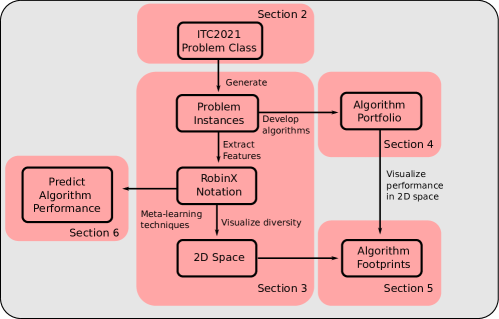
Figure 1: Building blocks of the algorithm selection framework.

2 Problem description

We envision the sports timetabling problem from the ITC2021 competition, which requires constructing a double round-robin tournament (2RR), meaning that each team plays against every other team exactly once at home and once away. Moreover, it assumes that the number of teams $n$ is even and that the timetable is compact (i.e., there are $2n-2$ time slots, or in other words, each team plays exactly one game per time slot). Furthermore, the ITC2021 problem instances feature nine (somewhat simplified) constraint types from the classification framework by Van Bulck et al [39]. Constraints are either hard or soft, where hard constraints represent fundamental properties of the timetable that can never be violated and soft constraints represent preferences that should be satisfied whenever possible. The objective in the ITC2021 problem instances is to minimize the overall (weighted) sum of deviations from violated soft constraints while respecting all hard constraints. In the remainder of this section, we describe each of the constraint types (grouped into four constraint classes), and refer to Van Bulck and Goossens [37] for a more detailed description of the constraints and their representation in the competition file format of RobinX.

Capacity constraints

The first class of constraints regulates when teams can play home or away.
CA1 constraints limit the total number of home or away games played by a given team during a given set of time slots, regardless of the opponent.
CA2 constraints limit the total number of home or away games played by a given team against a given set of opponents during a given set of time slots.
CA3 constraints limit the total number of home or away games played by a given team against a given set of other teams during each sequence of a given number of time slots.
CA4 constraints limit the overall number of home games (away games, or games) played by a given set of teams against a given set of other teams during a given set of time slots.

Break constraints

If a team plays two consecutive home games, or two consecutive away games, we say it has a break.
BR1 constraints limit the total number of breaks for a given team during a given set of time slots.
BR2 constraints limit the total number of breaks in the timetable. At most one constraint of this type (hard or soft) is present.

Game constraints

The third class consists of only one constraint type.
GA1 constraints enforce or forbid the assignment of a (set of) game(s) to one or more specific time slots.

Fairness and separation constraints

The last constraints aim to increase the fairness and attractiveness of the tournament, and are always soft. Moreover, there is at most one constraint of each type.
The FA2 constraint expresses the preference that the timetable is 2-ranking-balanced, meaning that the difference in the number of played home games between any two teams at any point in time is at most 2.
The SE1 constraint specifies that there are at least 10 time slots between any two games involving the same opponents.

Apart from these constraints, some problem instances also require that the timetable is ‘phased’, meaning that each team meets every other team exactly once in the first $n-1$ time slots and once in the last $n-1$ time slots.

3 Instance space analysis

To be suitable to compare the performance of algorithms, it is important that a benchmark is diverse in the sense that it covers the entire spectrum of properties found in real-life problem instances, otherwise there is the risk that the performance of the algorithms will not generalize well outside the benchmark. To assess the diversity of a given benchmark of problem instances, Smith-Miles and co-authors have developed a framework known as instance-space analysis (ISA) that, among others, can be used to visualize how similar or dissimilar problem instances are with regard to each other (see e.g. Smith-Miles and Lopes [32], Smith-Miles et al [33], Smith-Miles and Bowly [31], Kletzander et al [20], de la Rosa-Rivera et al [29]). The main idea behind their framework is that the similarity of problem instances can be assessed by comparing the associated ‘features’ (i.e., measurable properties) of the problem instances: two instances are considered similar if their features are also similar. In other words, we can represent instances in a high-dimensional feature space where each dimension corresponds to one feature, and subsequently we can assess how well the instances cover the entire high-dimensional feature space. To aid in visualization, Smith-Miles and co-authors suggest transforming the high-dimensional feature space into a two-dimensional (2D) space using dimensionality reduction techniques like Principal Component Analysis (PCA, see e.g., Abdi and Williams [1]).

Let us denote by $F$ the set of problem instance features. In order to generate a realistic and diverse set of problem instances for ITC2021, Van Bulck and Goossens [37] propose to use the number of teams in the problem instance as a first feature; a second feature indicates whether or not the competition is phased. Finally, one additional feature per hard and soft constraint type denotes how many constraints of that type are present in the problem instance. For instance, if a problem instance contains 20 hard constraints of type CA1, then $f_{\text{CA1}}^{H}=20$. For an overview of the features, we refer to Table 1. As already mentioned in the introduction of this paper, we categorize these features as ‘high-level’, and refrain from using more sophisticated features. Indeed, not only are such features often hard to explain to practitioners, they are also difficult to use for algorithm recommendations as practitioners do not know the precise details of the problem instances to be solved in the future.

Name	Description
$f_{|T|}$	Number of teams
$f_{\text{P}}$	Boolean which is one if the tournament is phased and 0 otherwise
$f^{H}_{\text{CA1}}$	Number of CA1 hard constraints (others: $f^{H}_{\text{CA2}}$, $f^{H}_{\text{CA3}}$, $f^{H}_{\text{CA4}}$, $f^{H}_{\text{GA1}}$, $f^{H}_{\text{BR1}}$, $f^{H}_{\text{BR2}}$)
$f^{S}_{\text{CA1}}$	Number of CA1 soft constraints (others: $f^{S}_{\text{CA2}}$, $f^{S}_{\text{CA3}}$, $f^{S}_{\text{CA4}}$, $f^{S}_{\text{GA1}}$, $f^{S}_{\text{BR1}}$, $f^{S}_{\text{BR2}}$, $f^{S}_{\text{FA2}}$, $f^{S}_{\text{SE1}}$)

Table 1: Overview of the 18 features in $F$ considered for the instance generation of the ITC2021 competition.

Van Bulck and Goossens [37] show how these high-level features can be used to represent the ITC2021 problem instances in a 2D instance space using PCA (after applying min-max normalization and mean-centring of the feature values). The result is depicted in Figure 2, where the red convex hull corresponds to what Van Bulck and Goossens [37] call the ‘target instance space’, defining the region in the 2D instance space where real-world problem instances are likely projected. As a result from mean-centring, the features reach their average near the origin of the instance space. The ITC2021 competition offers a benchmark of 45 highly-constrained problem instances, with 16, 18, or 20 teams. Since a set of 45 problem instances is quite limited to apply machine learning tools, we use the method described by Van Bulck and Goossens [37] to produce a diverse set of 518 additional challenging and realistic problem instances. In the remainder of this paper, the set of 45 competition instances is referred to as ITC2021, and the set of 518 additional problem instances as Additional. Figure 2 shows that the ITC2021 as well as the additional problem instances cover the 2D space very well, suggesting that the problem instances are representative for the wide variety of round-robin tournaments found in real-life (see also Van Bulck and Goossens [37]).

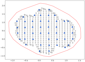
Figure 2: Projections of the problem instances in the two-dimensional instance space. The additional and ITC2021 competition problem instances are represented by gray circles and blue triangles, respectively.

In order to gain insights into the composition of the 2D instance space, Figure 4 shows the distribution of the (non-normalized) feature values. The figure shows that there is a large variety in the number of constraints of each type that are present. For instance, we observe that there can be up to 600 CA2 soft constraints, while none of the problem instances have more than two CA3 hard constraints. We also observe that most of the feature values follow a linear trend over the instance space. For instance, the problem instances with a BR2 hard constraint are in the top left whereas those with a BR2 soft constraint are almost all in the bottom right. Similarly, phased problem instances are located in the left of the instance space whereas regular problem instances are located near the right. For the number of teams, however, no linear structure can be observed (this was by construction, see Van Bulck and Goossens [37]).

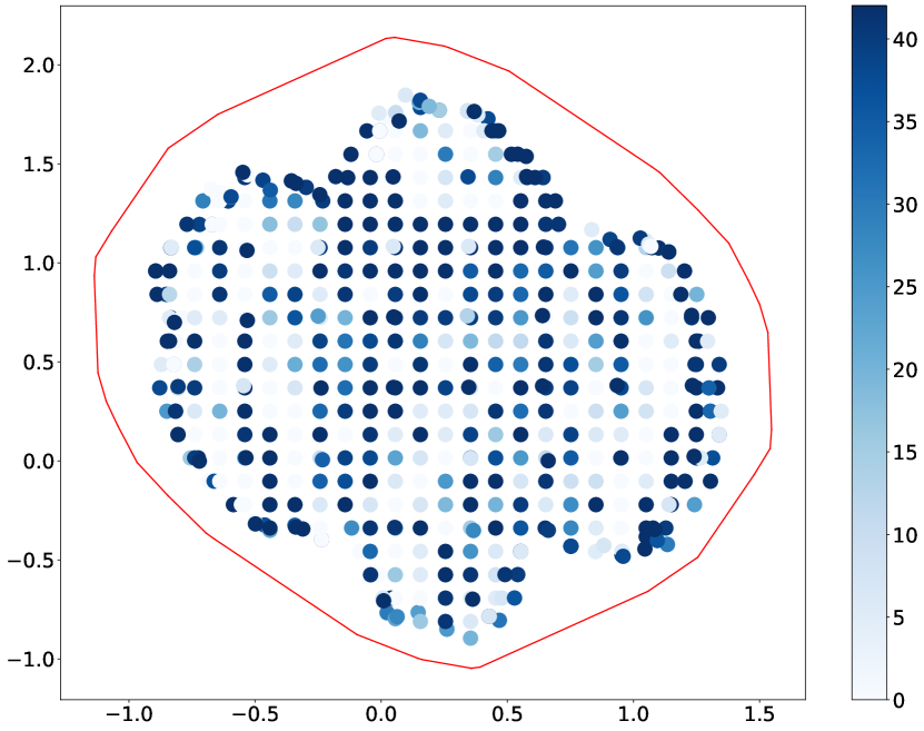
(a) CA1 Hard

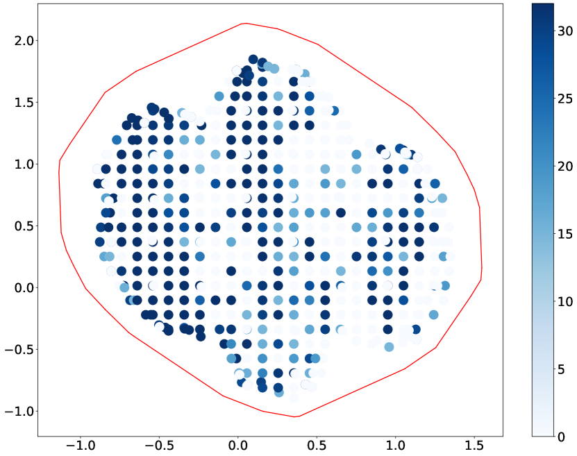
(b) CA1 Soft

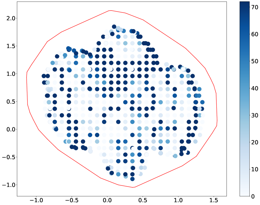
(c) CA2 Hard

(d) CA2 Soft

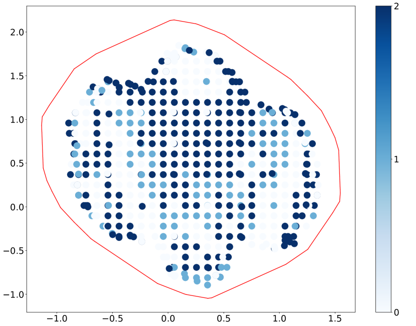
(e) CA3 Hard

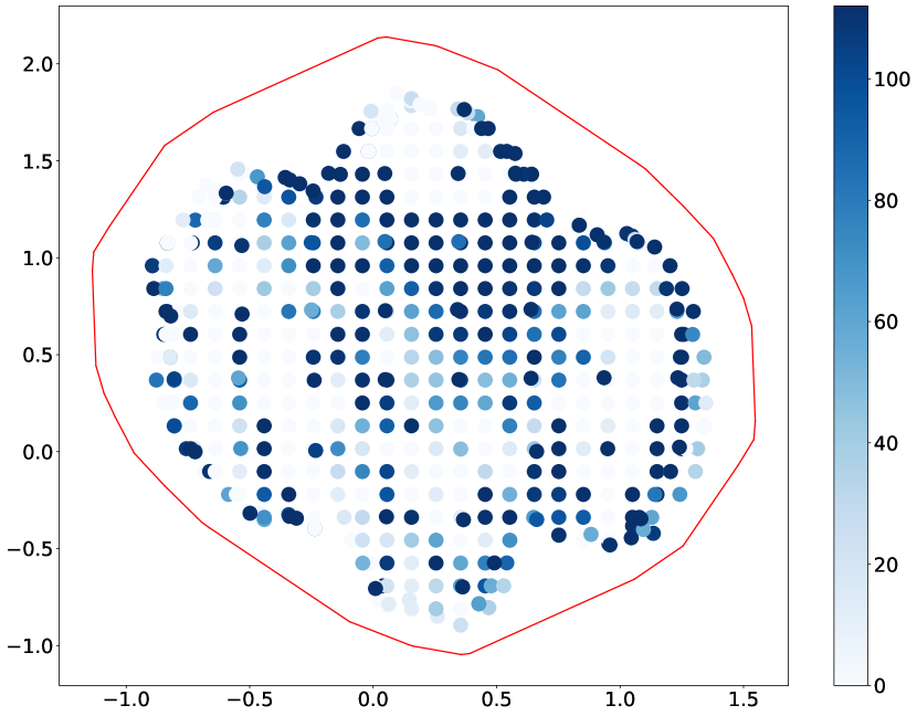
(f) CA3 Soft

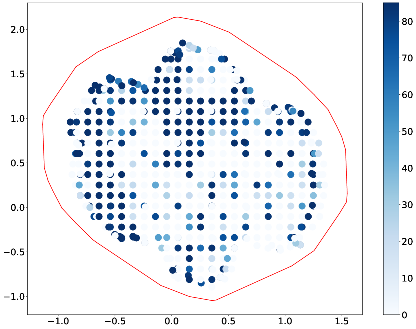
(g) CA4 Hard

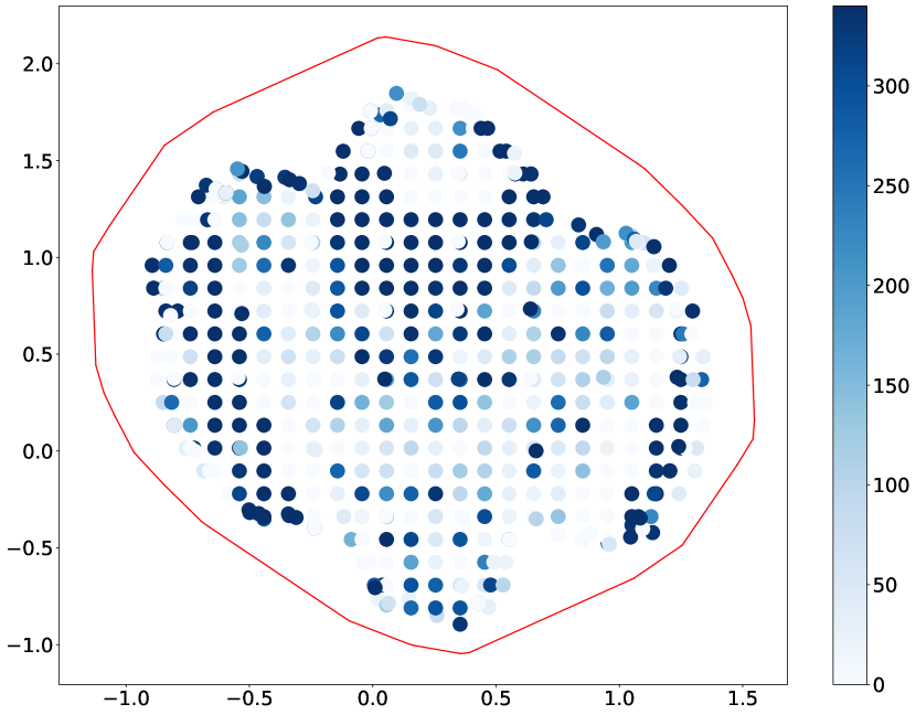
(h) CA4 Soft

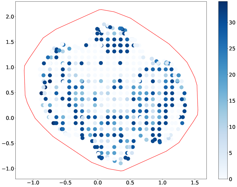
(i) GA1 Hard

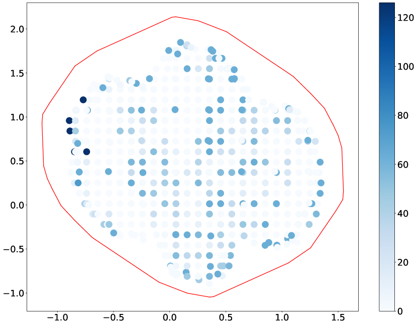
(j) GA1 Soft

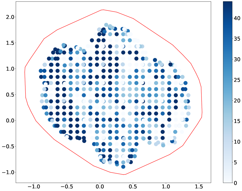
(k) BR1 Hard

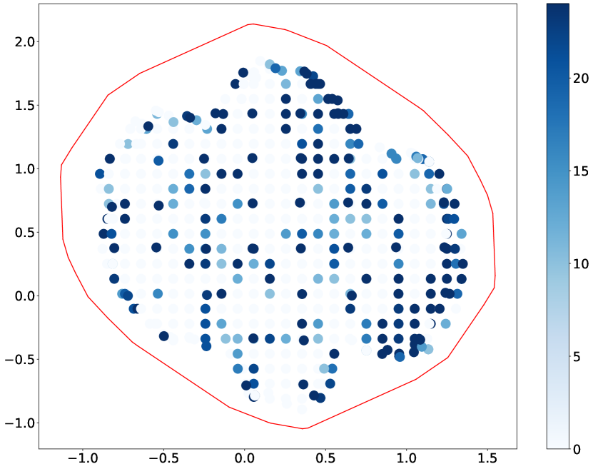
(l) BR1 Soft

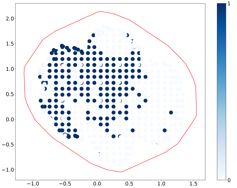
(a) BR2 Hard

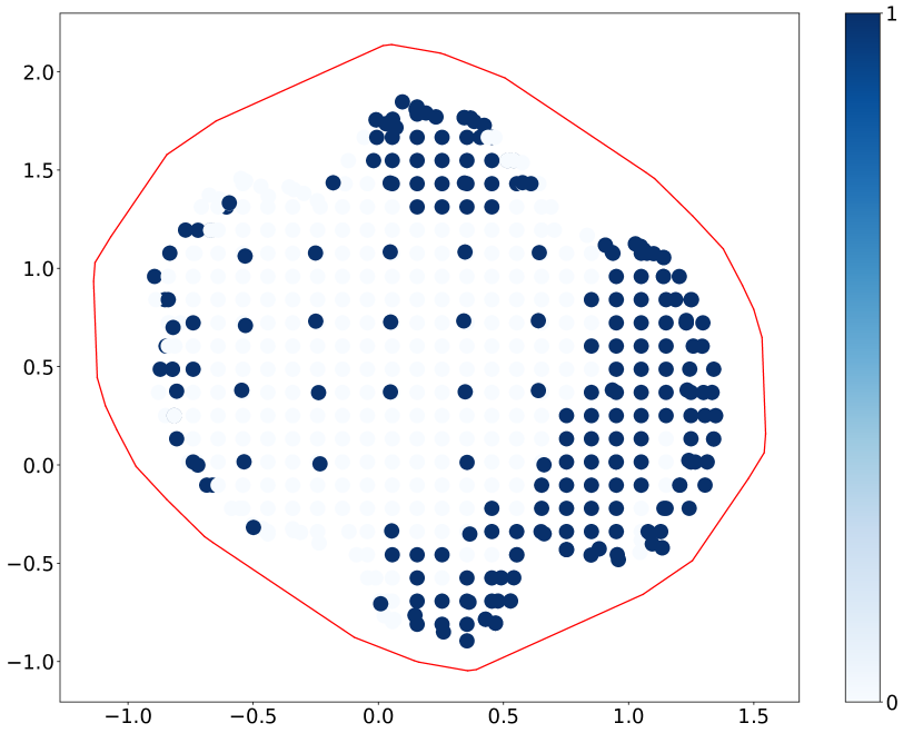
(b) BR2 Soft

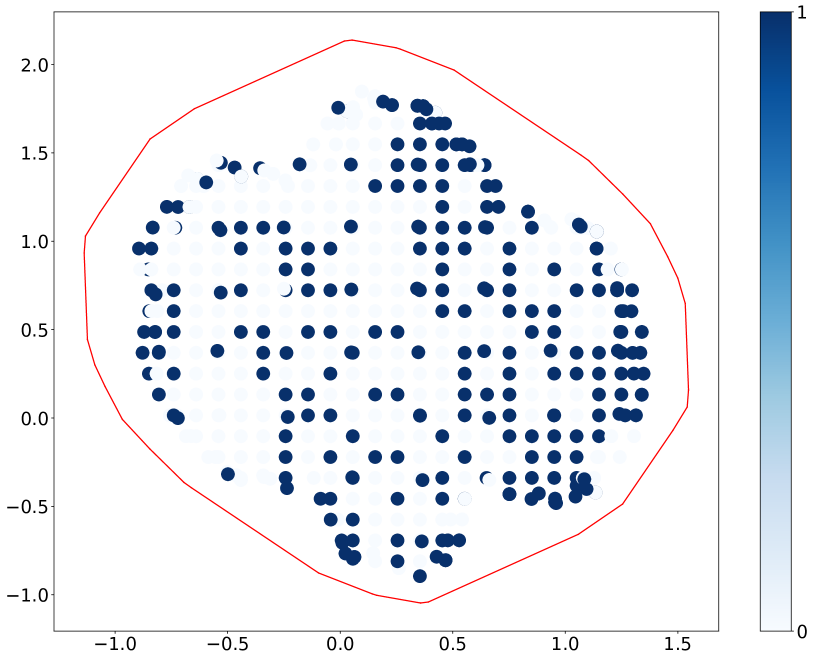
(c) FA2 Soft

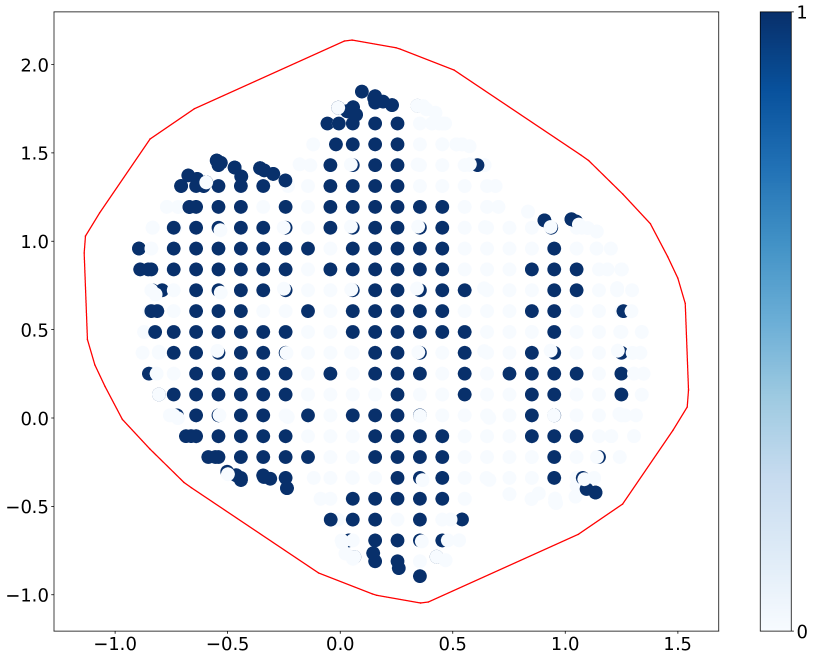
(d) SE1 Soft

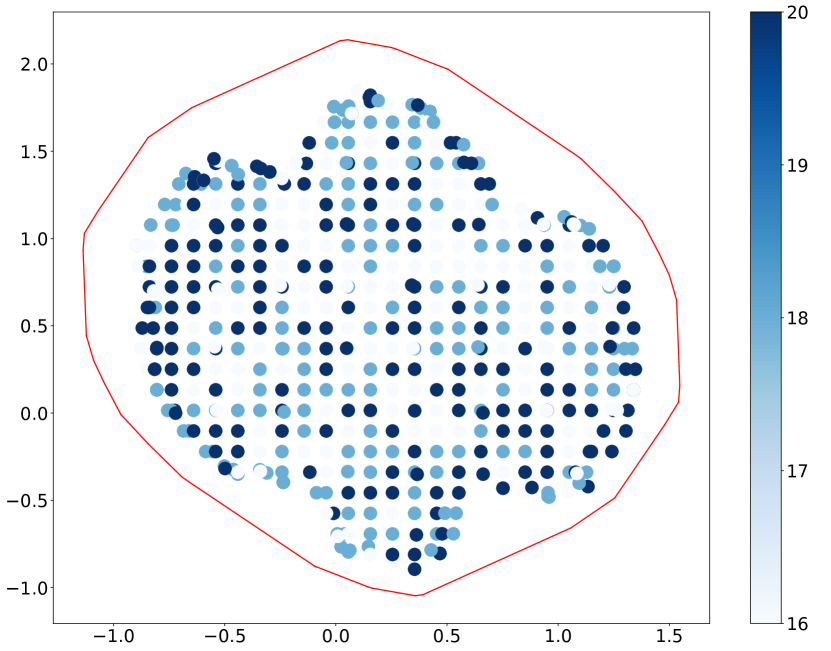
(e) Number of teams

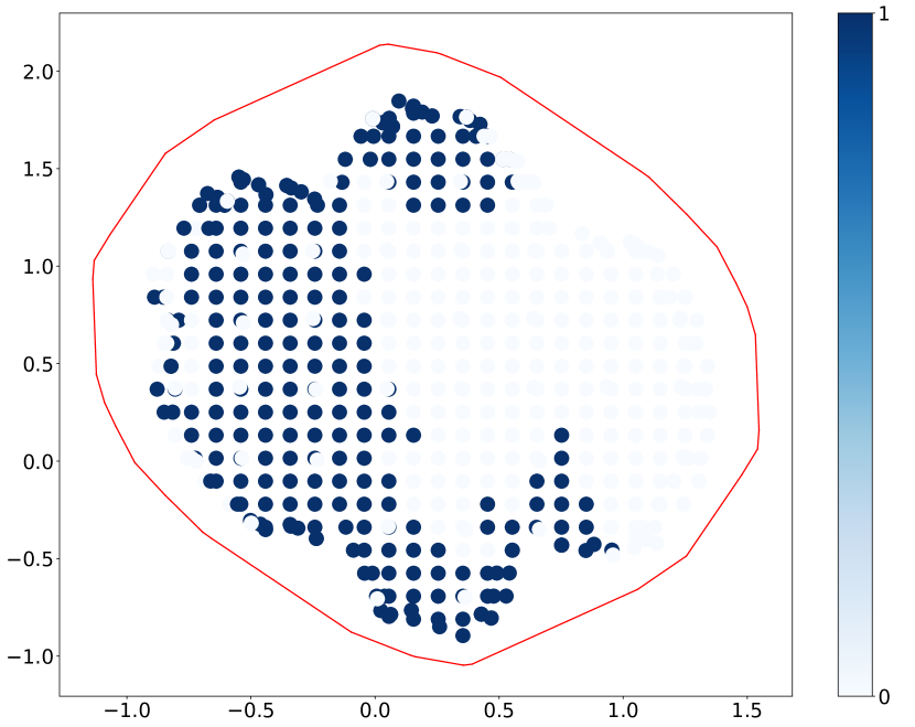
(f) Phased

Figure 4: Instance space analysis: distribution of the non-normalized instance features values among the two principal component axes.

4 Sports timetabling algorithms

This section provides a short description of eight state-of-the-art algorithms that were developed for solving sports timetabling problem instances in the ITC2021 format. For an overview of the algorithms and their implementation details, we refer to Table 2.

4.1 MODAL

Berthold et al [4] model the problem as a Mixed-Integer Program (MIP) and propose a solution strategy, coined MODAL, based on an ensemble approach employing different MIP solvers (Gurobi, CPLEX, Xpress). The choice for an ensemble approach is twofold. Firstly, as MIP solvers have different strengths, some solvers may be more suitable than others depending on the problem instance to be solved. The second reason is to exploit the effect of performance variability: instead of computing solutions in single long runs, the solvers are called repeatedly, starting with the best found solution in each iteration.

As finding an initial solution can be challenging, two start procedures have been implemented. The first one uses an analytic centre objective. It replaces the objective function of a MIP by coefficients that correspond to the analytic centre of the polyhedron associated to the MIP. The second uses a version of the feasibility pump with multiple integer reference vectors (see e.g. [3]).

Using a dedicated cluster facility, MODAL was run for each instance up to 25 times, using an overall time limit of up to 10 hours. In addition, for a few cases, a framework for computing MIPs on massive parallel distributed memory super computers was employed. The parameters were varied between the runs, usually increasing the number of heuristic runs, emphasizing on finding feasible solutions, reducing the amount of cutting plane generation, etc. Note, though, that all instances went through the same loop of repeated solving by various solvers, with the amount of loops depending on the solution quality. Similarly, whether we applied heuristic methods to ignite the search depends on whether the initial MIP searches yield a feasible solution, but not on any of the problem characteristics.

The catch of MODAL is that it does not use any special purpose timetabling algorithm. All methodology is general MIP technology, available independently of this work.

4.2 Goal

The Goal algorithm proposed by [13] is based on the fix-and-optimize strategy, which may be categorized as a matheuristic. Matheuristics are heuristics that take advantage of the power of mathematical programming solvers to tackle hard combinatorial optimization problems. More specifically, fix-and-optimize algorithms are matheuristics that iteratively employ a mathematical programming solver to optimize a small subproblem while the remainder of the problem remains fixed.

Goal selects, at each iteration, a subset of the time slots to compose the subproblem. Their related variables are released while the others are fixed to their current values. Variables related to the inversed venue games are also released to allow venue exchange. Hopefully, in a given iteration, a better solution will be found by the IP solver by exploring the possibility to exchange several variables simultaneously and efficiently. The subproblem size is auto-adjusted throughout the execution of the algorithm, while the time limit for each iteration was empirically set to 100 seconds.

Fix-and-optimize algorithms require an initial solution to heuristically improve. In this case, the canonical factorization from de Werra [41] is used to generate an initial solution. Given this initial solution, the proposed algorithm executes twice: first to obtain a feasible solution and then to refine (improve) this solution. Only hard constraints, modelled as soft constraints, are included in the first execution. When a feasible solution (zero-cost) is found, the second execution begins, taking this feasible solution as input. In the second execution, all slack variables for hard constraints are removed and the soft constraints are added to the model.

Goal was implemented in Java 16. Gurobi 10.0 with MIPFocus set to feasibility was employed to solve the subproblems in the fix-and-optimize algorithm. For each available instance, the algorithm ran on a single thread of an Intel Core i7-8700 3.2GHz with 12 GB RAM. The considered stopping criterion is a run-time limit of 24 hours. The algorithm may also be interrupted when optimality can be asserted - a zero-cost solution has been found or the subproblem size matches the problem size and the subproblem solution is optimal.

4.3 DES

The DES algorithm proposed by Phillips et al [25] uses an Adaptive Large Neighbourhood Search (ALNS) matheuristic. This can equivalently be described as a fix-and-optimize method, with the addition of an adaptive control strategy from the field of reinforcement learning.

To generate a starting solution, DES first attempts to solve a monolithic integer program. If unsuccessful after a fixed time, it reverts to using the canonical factorization from de Werra [41]. The remaining time is spent applying the ALNS technique where only part of the solution may be modified in each iteration. An IP is solved within each neighbourhood subproblem, aiming to minimise the number of hard and soft constraint violations. The neighbourhood definition is adaptively chosen from a set of different types and sizes, based on results of previous iterations. This is treated as a multi-armed bandit problem, using the upper confidence bound method [34]. Each neighbourhood type (‘arm’) is chosen as that with the greatest optimistic upper bound on its expected probability of improving the solution (‘reward’). This balances between exploring different neighbourhood types and exploiting those which have already performed well. We found that searching a larger number of small neighbourhoods was the most effective.

4.4 UoS

The UoS matheuristic approach proposed in [21] is also based on an IP formulation of the problem. The algorithm starts from a solution that has a valid schedule structure for a (phased) double round robin tournament, obtained with a reduced IP formulation. A Variable Neighbourhood Descent (VND) framework is then used to explore five neighbourhoods that consist of IP models in which some variables are fixed. Three of the neighbourhoods look at fixing most of the variables in a current solution, except variables relating to selected sets of $c_{1}$ slots, $c_{2}$ teams, and $2$ teams and $\frac{c_{1}}{2}$ slots, where $c_{1}$ and $c_{2}$ are hyperparameters of the algorithm. The two remaining neighbourhoods optimize one phase of the competition in full and the home team of matches, respectively. To diversify the search at local optima, the objective function coefficients of most violated constraints increase, prompting the algorithm to move to other parts of the search space. The full IP formulation of the problem, and more details of the algorithm and its neighbourhoods are reported in [21].

For this article, the algorithm was divided into two phases: feasibility search, and improvement search. The feasibility search phase tackled the problem discarding all soft constraints but aiming to minimise breaks, and applied the VND matheuristic for $25\%$ of the time. During this phase, models were solved only for up to two seconds. If a feasible solution was found, the algorithm moved to the improvement phase, otherwise the feasibility phase was extended until a feasible solution was found with ten seconds. The improvement phase applied VND with the full model for the remaining time. For all instances, we performed five different 48-hour runs in computer nodes with dual 2.0 GHz Intel Skylake processors enabled with 4 cores, with slight variations of hyperparameters. Four runs were set up with $c_{1}=12$, $c_{2}=8$ and time limits from 10 to 60 seconds. The fifth run considered smaller models with $c_{1}=10$, $c_{2}=6$ and a 15 second time limit.

Finally, a further 24-hour run with 20 cores was set up for those instances that remained infeasible after the above procedure. Here, the algorithm used in the feasibility search was slightly different, with the intention of tackling larger problems. In this version, the problems are decomposed in stages, each stage considering 200 constraints more than the previous stage. Only when all the constraints of a stage are satisfied, the next 200 are added to the model, prioritised so that the most violated constraints are added first. Further, the selection of slot sets in our neighbourhoods included evaluating a few options (5 in our experiments) by means of the lower bound provided by their linear relaxation. The algorithm then selects the set in which this value is lower. If none of the values improves the current best solution, more sets are generated, potentially modifying the number of slots in the set (effectively adapting the value of $c_{1}$).

4.5 Udine

The metaheuristic proposed by [30] employs a portfolio of six local search neighbourhoods: SwapHomes, SwapTeams, SwapRounds, PartialSwapTeams, PartialSwapRounds, and PartialSwapTeamsPhased. While the first five neighbourhouds were previously proposed in the literature [see 2], the last one is novel and works by performing a partial swap among the opponents of two teams in (a part of) the timetable, but in such a way that the phase constraint does not become violated (possibly requiring additional swaps of the home advantage). PartialSwapTeamsPhased proved its effectiveness especially with regard to phased instances, but it is useful, according to experimental data, also on non-phased ones.

The neighbourhoods are combined via simulated annealing, making use of a so-called cut-off mechanism to speed up the early phases of the search [see 18]. The search is performed in three sequential simulated annealing runs, called stages, that are aimed, respectively, at finding a feasible solution that does not violate hard constraints, at exploration and exploitation by navigating both the feasible and the infeasible region, and at finding a better local minimum by just exploring the feasible region. The first stage starts from a greedily-constructed solution, every next stage is warm-started by the best solution found in the previous one. In line with [30], the stages always execute a given number of local search evaluations, so there is no fixed time limit. The resulting running times vary noticeably, as the time spent for the evaluation of local search moves depends on the size of the instance and on the number of constraints.

4.6 DITUoIArta

DITUoIArta is a hybrid approach, where an exact solver is combined with a metaheuristic [9]. The exact solver of choice is the open-source Google ORTools CP/SAT that holds the distinctiveness of expressing a model in Constraint Programming (CP) terms, with the solver reformulating the problem in a satisfiability (SAT) model. The latter seems to be better adapted to the overly constrained nature of sports timetabling. For the local search, simulated annealing is used with five neighbourhood operators proposed in the literature, namely SwapHomes, SwapRounds, SwapTeams, PartialSwapTeams and PartialSwapRounds [2].

Using CP/SAT, an initial solution that satisfies the base constraints is created. Hard constraints are interpreted as soft constraints, while the original soft constraints are ignored. Simulated annealing attempts to place the solution into the feasible space. If a feasible solution is found, hard constraints become mandatory and soft constraints are turned on. Every time the simulated annealing seems unable to make progress, a CP/SAT improvement process tries to make the present solution better. To do this, a certain number of teams, slots, games, or some combinations of the aforementioned is randomly chosen and kept fixed, while the rest of the current solution is free to change. Finally, the whole process stops if an optimal solution is found either because it has no cost or the solution for the whole problem without fixed parts is reported optimal by the solver. A secondary stopping criterion also exists: if a solution remains unimproved for ten minutes the whole process stops.

Note that in all problem instances there are at most two hard CA3 constraints, one for home games, and one for away games. However, if both constraints appear, then no team can have two breaks in a row. By providing this information to the CP solver early and tightening the model, we were able to find better solutions or feasible solutions for instances that incorporate both hard CA3 constraints.

4.7 Reprobate

Reprobate [23] generates a monolithic encoding of the timetabling problem as a weighted pseudoboolean (PB) constraint optimization problem and applies a portfolio of off-the-shelf PB solvers. PB constraints are a generalisation of boolean satisfiability (SAT) constraints over boolean variables. Many relationships involving finite sets, such as set membership, subset and set cardinality, have a succinct encoding in this format, which makes it well-suited to a range of discrete optimization problems. Furthermore, PB constraints are equivalent to 0-1 integer programming. However, compared to MIP solvers, PB solvers tend to be stronger on problems solvable using mainly boolean reasoning, but weaker on problems where heavy use of arithmetic reasoning is required. Reprobate also tries some variations on the default encoding and applies a single solver to those.

If a feasible solution is found, and somewhat in line with the well-known paradigm of first-schedule-then-break (see Trick [35]), Reprobate attempts to improve the objective by encoding and solving a second optimization problem in which the allocation of opponents in each slot is fixed, but which team plays home in each game is not, effectively allowing the home away pattern (HAP), i.e a team’s succession of home and away matches, to be tuned. Again, this is a PB constraint problem.

For this study, we updated the portfolio of solvers used in Reprobate. We stick with clasp [15] (running with the crafty preset) as the default solver, but update it to version 3.3.9. Sat4J remains in the portfolio, but only with the specialist PB algorithms [22] introduced in version 2.3.6; the default setting is no longer used, as its performance was poor. In its place, we use the latest version of RoundingSat [12], using toyconvert to translate between the WBO format (produced by Reprobate) and OPB format (consumed by RoundingSat). We compiled RoundingSat without the optional Soplex integration, as it seemed to degrade performance on the benchmarks we tested; this also means that all the code and solvers remain available under permissive open source licences.

We ran all problem instances on a machine with an Intel Core i7-8700 CPU at 3.20GHz with 64 GB of RAM. Each solver instance was run on a single core with a time limit of 10 minutes. With 6 solvers on the default encoding, 7 encoding variations with the default solver and up to 2 tuning phases, this gives a total time limit of 150 minutes. In practice, it was rare to exceed 140 minutes, as one encoding variation (ignoring all soft constraints) often led to a solution in a few seconds, and when it did not, there was often no feasible solution to tune.

4.8 FBHS

Instead of constructing a timetable all at once, the first-break-heuristically-schedule (FBHS) algorithm proposed by Van Bulck and Goossens [36] considers the following subproblems which are sequentially solved: (i) determine for each team in every time slot whether it plays home or away (i.e., its HAP), and (ii) determine the opponent of each team in every time slot (opponent schedule). These two steps, though, must be compatible: two teams can only play against each other in the opponent schedule when one team plays home and the other team plays away according to their HAPs. It is important to realize that a HAP set does not necessarily allow a (high-quality) compatible opponent schedule that schedules all required matches (see e.g. [5]). Hence, to generate the HAP set, we use a traditional Benders’ decomposition approach that enforces some necessary HAP set feasibility conditions while also considering the LP-relaxation of the best possible opponent schedule.

The time limit for the HAP set generation process was set to 6 hours of computation time (wall time), using a total of 8 cores at the same time. Given the most promising HAP set found in step 1, we then construct a compatible opponent schedule using a fix-and-optimize matheuristic (a time limit of two minutes per IP model was imposed). The matheuristic was repeated for a total of 24 times, each run enabled with one core and solving 8 runs in parallel. On average, the compatible opponent schedule generation took 13.5 hours (a total time limit of 24 hours per instance was enforced).

Algorithm	Search method	Software details	Hardware details	Clock speed ratio
MODAL	IP Branch & Cut	Python, Zimpl, C, Gurobi 10, Xpress	Per instance one thread was used and several instances where run at the same time on a machine with a 24 core / 48 hyperthread Intel(R) Xeon(R) Gold 6342 CPU at 2,80 GHz	2.8/3.9
Goal	Fix-and-optimize matheuristic	Java 16, Gurobi 10.0	Intel Core i7-8700 3.2GHz with 12 GB RAM (single thread running for 24 hours per instance)	3.2/3.9
DES	Adaptive LNS matheuristic	Python 3.10, Gurobi 10.0	Intel Xeon 3.9GHz with 4 cores and 8 threads (Google Compute Engine “c2-standard-8”) for 2.5 hours per instance	3.9/3.9
UoS	VND matheuristic	Python 3.10.4, Gurobi 9.0.2	Dual 2.0 GHz Intel Skylake with 4 or 20 cores	2.0/3.9
Udine	Simulated annealing	C++17	Intel Xeon Processor (Cascadelake) @ 2.4 GHz, 16 cores, (max one core per execution)	2.4/3.9
DITUoIArta	CP/SAT + Simulated annealing	Python 3.10, ORTools 9.4	6 x Intel Core i5-10505 @ 3.2 GHz with 8GB RAM (all cores activated for the solver only) for 1 hour each time for each instance (an instance may run multiple times though)	3.2/3.9
Reprobate	Pseudoboolean optimization	Perl, clasp 3.3.9, Sat4J 2.3.6, RoundingSat Git Nov 2022	Intel Core i7-8700 3.2GHz with 64 GB RAM (single core running for 2.5 hours per instance)	3.2/3.9
FBHS	IP Decomposition + matheuristic	C++, CPLEX 12.10	Intel Xeon E5-2660v3 (Haswell-EP @ 2.6 GHz) processor enabled with 8 cores	2.6/3.9

Table 2: Overview of algorithms together with software and hardware details. The last column compares processor clock speeds relative to the ‘fastest’ processor used (3.9 GHz).

5 Computational results

Section 5.1 explains the criteria used to compare the algorithms and gives more details on the running times. Next, Section 5.2 provides an overview of computational results and constructs the algorithm footprints. In Section 5.3, we have an empirical assessment of the hardness of the instances.

5.1 Experimental setting

All algorithms described in Section 4 were given two weeks of time to produce best found solutions for all additional problem instances. The algorithms, which in most cases differ somewhat from their ITC2021 implementation, were also rerun on the ITC2021 competition instances. Besides the overall two-week time limit, there were no limits on the computation time for individual problem instances, nor on the number of cores or computing infrastructure used. This choice is motivated as follows. First of all, computation time is rarely a critical issue in sports timetabling: practitioners typically have several days or weeks to produce the fixtures. Second, the overall two week time limit corresponds to the criterion used for the late instances of the ITC2021 competition, allowing us to use algorithm code as-is. Indeed, many of the algorithms developed for the ITC2021 competition did not use an explicit time limit but rather stopped the search when no improvement was found for a given number of iterations. Finally, for practical reasons, each algorithm was run on the infrastructure available at the institution where it was developed. The available hardware sometimes differs substantially: while some algorithms could handle several instances in parallel, having more than 20 cores available, others tackled the whole instance set with a single core. We are aware that these differences in computing infrastructure can bias the performance comparison and even influence the recommendations of which algorithm to use. Nevertheless, maintaining this ITC2021 rule, which gave full freedom in the use of computational infrastructure, was a necessity given the size of our computational experiment.

Figure 5 provides an overview of the wall times (i.e., the total execution time of the code) and CPU times (i.e., wall time multiplied with the number of cores used) used by the various algorithms. The figure shows that wall times can be categorized into three groups: short (up to several hours: DES, DITUoIArta, Reprobate, and MODAL), medium (about a day: Goal, FBHS, Udine), and long (several days: UoS). Some of these differences are substantial, however, we point out that in sports timetabling, the quality of the timetable is much more important than the speed of computation [37].

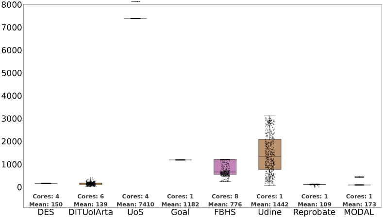
(a) Wall time (minutes)

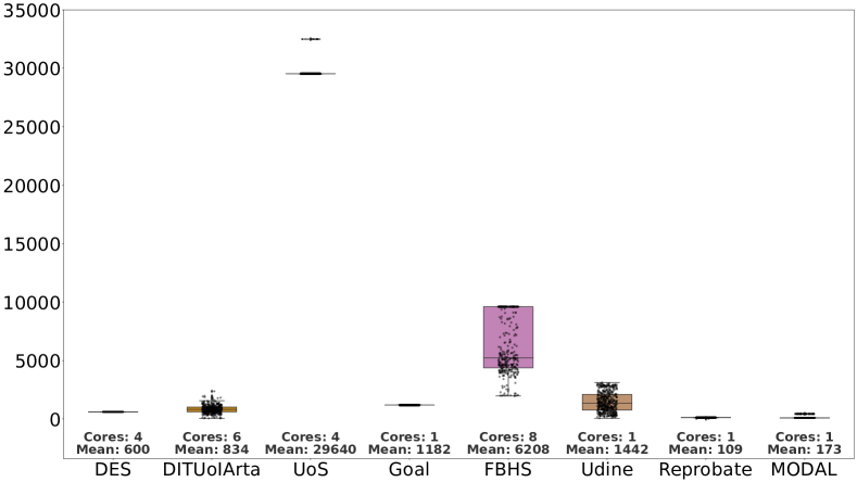
(b) CPU time (minutes)

Figure 5: Distribution of the runtimes for the additional problem instances per algorithm. For each algorithm, only instances for which it found a solution are considered. Runtimes are normalized with regard to processor clock speed by multiplying with the clock speed ration from Table 2.

5.2 Algorithm performance

In order to compare the performance of the algorithms over the problem instances, Figure 6 shows the winning algorithm in terms of the best solution found for each of the problem instances. The figure shows that most of the algorithms perform particularly well in a specific part of the instance space (which is a first indication of the potential of algorithm selection). For example, we see that the FBHS solver performs exceptionally well near the right side of the instance space where there are many BR2 soft constraints (see Figure 4). In contrast, Goal scores well near the origin of the instance space where, as a result from the mean centring, instances have more or less average feature values. It is also interesting to note that all problem instances for which no algorithm found a solution are located near the left of the instance space. This part of the instance space corresponds to problems that are phased, and have a SE1 soft and a BR2 hard constraint.

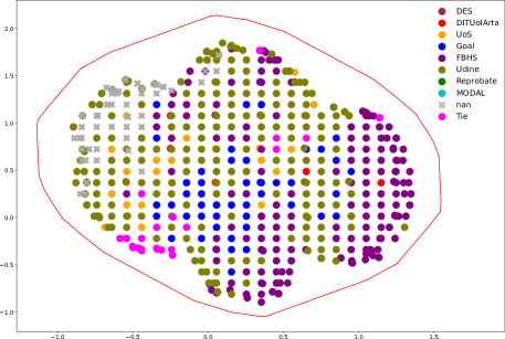
Figure 6: Overview of best performing algorithm for each of the additional problem instances. Problem instances for which none of the algorithms found a solution are indicated by a gray x-mark.

While Figure 6 provides an overview of where each algorithm works best, it does not show the relative performance between the different algorithms. To address this, let us define with $p_{i,a}$ the quality of the best found solution by algorithm $a$ on problem instance $i$, and the absolute gap of algorithm $a$ on instance $i$ as $\Delta_{i,a}$, where $\Delta_{i,a}$ is calculated as the difference between $p_{i,a}$ and the best performance achieved across all algorithms on instance $i$ (i.e., $\Delta_{i,a}=p_{i,a}-\min_{a}p_{i,a}$). In case no solution was found, we set $p_{i,a}=\Delta_{i,a}=\leavevmode\hbox to4.2pt{\vbox to4.2pt{\text{[drawing]}}}$. Figure 7 shows the number of problem instances for which $a$ found a feasible solution as well as the distribution of $\Delta_{i,a}$ among these problem instances. The figure shows that Udine managed to find a solution for the largest number of instances, and that these solutions are never very far from the best found solutions. While the absolute gap is only slightly larger for the FBHS solver, it terminated without having found a feasible solution for a considerably larger number of instances. Compared to the other solvers, the gap for DITUoIArta, DES, and Reprobate is larger but we remind the reader that these solvers were run on a fairly modest computing infrastructure.

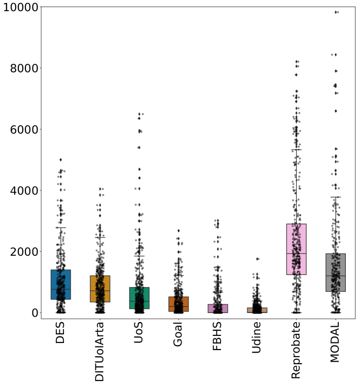
(a) $\Delta_{\text{i,a}}$

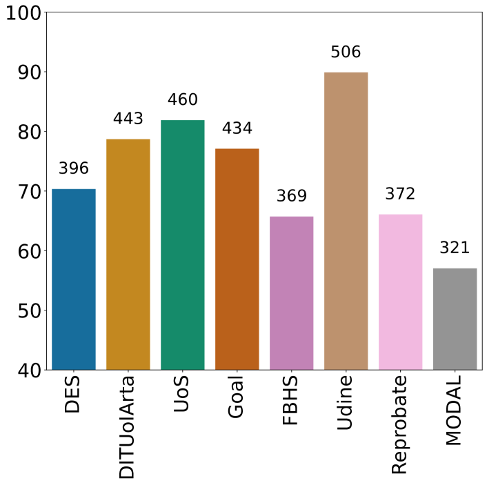
(b) Feasible solutions

Figure 7: Distribution of $\Delta_{\text{i,a}}$ and the percentage of problem instances for which a solution was found. The number on top of each bar denotes the absolute number of solutions found.

In order to be able to easily compare $\Delta_{i,a}$ across different problem instances, we normalize $\Delta_{i,a}$ to the range $[0,1]$ by using the relative gap $\epsilon_{i,a}=1-\Delta_{\text{i,a}}/p_{i,a}$ instead. If no solution was found we set $\epsilon_{i,a}=\leavevmode\hbox to4.2pt{\vbox to4.2pt{\text{[drawing]}}}$, otherwise $\epsilon_{i,a}$ thus gives how close $a$ gets to the best known solution with higher values considered to be better. Figure 8 uses a non-linear color scheme to superimpose the relative gap of the algorithms in the 2D instance space, highlighting for each algorithm where it performs exceptionally well. Several algorithm recommendations can be distilled from these so-called algorithm footprints.

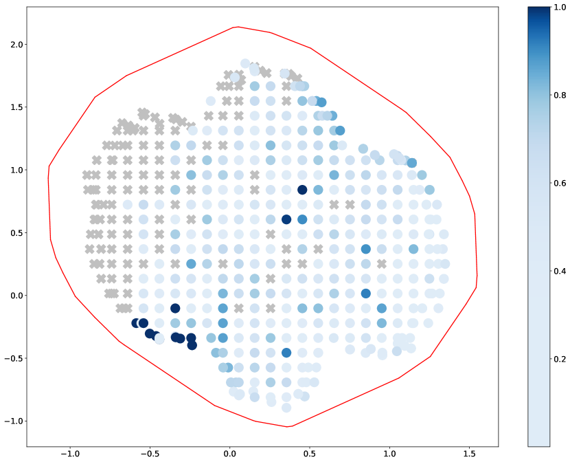
(a) DES

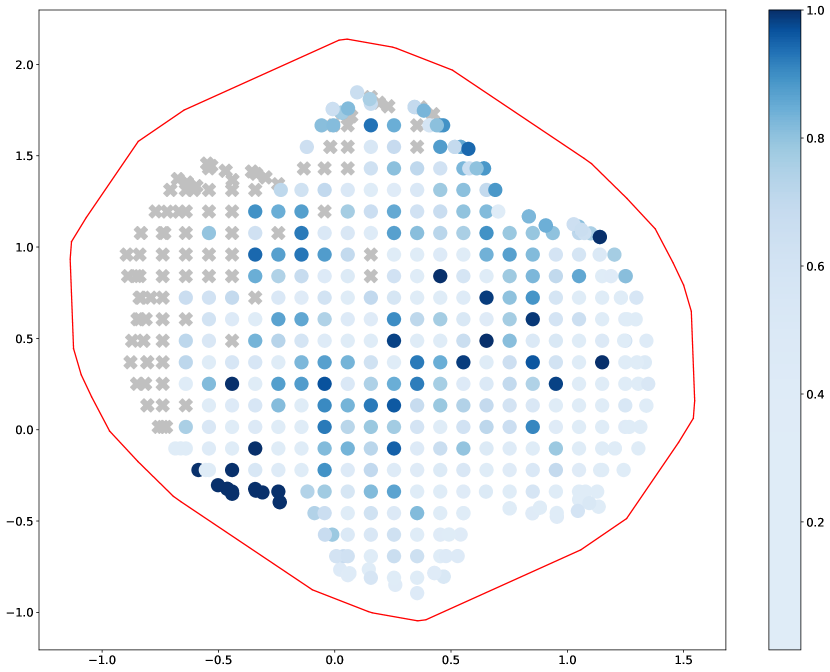
(b) DITUoIArta

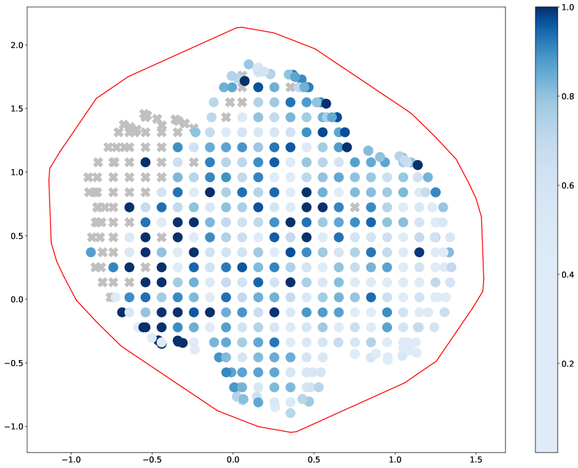
(c) UoS

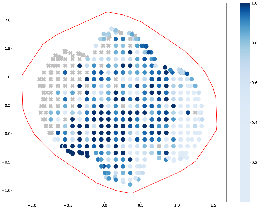
(d) Goal

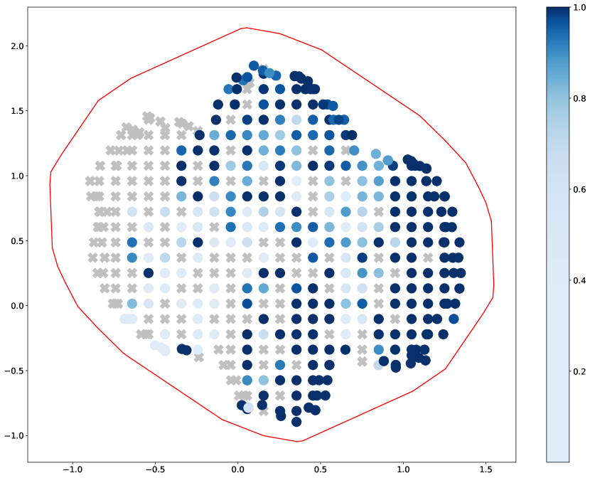
(e) FBHS

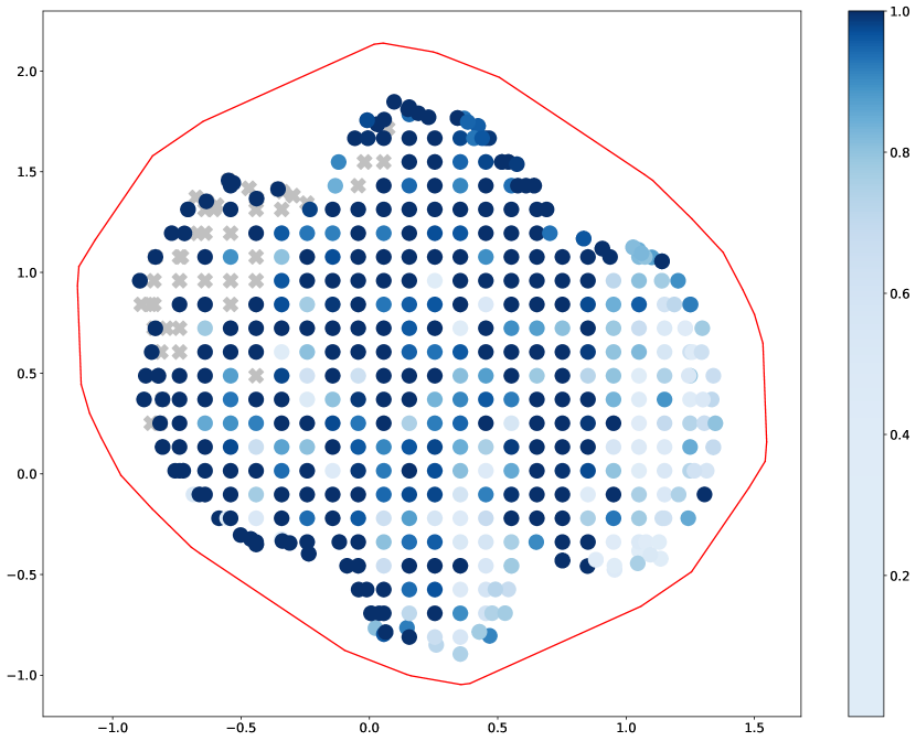
(f) Udine

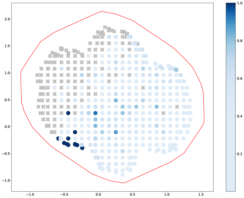
(g) Reprobate

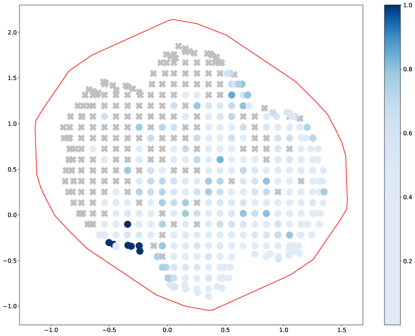
(h) MODAL

Figure 8: Algorithm footprints. Problem instances for which no feasible solution was found are indicated by a grey x-mark.

Reprobate and MODAL behave quite similarly. Both struggle with finding best solutions. Indeed, even a clever combined approach of state-of-the-art solvers and use of a substantial computational effort results in no more than a handful of instances where MODAL tops the other algorithms. This suggests that complex sports scheduling problems are still beyond reach for IP solvers. MODAL also displays the lowest number of instances for which a feasible solution was found. Its footprint indicates that finding a feasible solution is particularly hard for problem instances in the top left area of the instance space. While Reprobate does not do better with respect to best solutions, it does manage to find a feasible solution for more problem instances, suggesting that constraint satisfaction techniques are more suited for this than IP models. Recall that Reprobate is based on pseudo-boolean (PB) optimization and that its main idea is to provide solutions with off-the-shelf generally applicable PB solvers. Nevertheless, Reprobate also fails in the region corresponding to phased problem instances that have a SE1 soft and a BR2 hard constraint. Considering an alternative PB constraint formulation for these constraints may thus be a way to further improve this algorithm.

Although DITUoIArta and DES are rather different algorithms and DITUoIArta finds more feasible solutions than DES, the footprints of these algorithms are also quite similar. They were also run on a similar infrastructure, which granted them a rather short running time per instance. Their footprints display excellent results in the bottom left area, and occasional high-quality solutions along the 45^∘ diagonal. Beyond that region, both algorithms struggle, but we cannot rule out that they perform better on high-end hardware. In fact, after the conclusion of the ITC2021 competition, this was illustrated by DES finding several new best solutions by employing considerably longer running times than used for the experiments of this paper.

The solvers UoS and Goal are alike in the sense that they are both matheuristics. It is interesting to see that both of them perform particularly well along the bottom-left to top-right diagonal of the instance space. None of the instance features seem to really dominate in this region, meaning that instances across this diagonal could be considered as ‘average instances’. The two solvers still find a significant number of feasible solutions in other regions of the instance space, though, the quality of these solutions is somewhat less promising.

With regard to the FBHS solver, we observe that if a solution is found, it is very often close to the best known solution, especially when the number of breaks is to be minimized (BR2 soft constraint). Specifically designed to cope well with breaks, it is somewhat surprising, though, that this solver has difficulties to find feasible solutions for the case where most of the break constraints are hard. Moreover, the solver also seems to struggle with problem instances that are located near the middle of the instance space. As the FBHS solver constructs a timetable in two phases, it would be helpful to figure out whether the solver fails to find a feasible solution because the generated HAP set is infeasible, or rather because the matheuristic of the second phase fails to find a compatible opponent schedule even though the HAP set is in fact feasible. In the latter case, replacing the matheuristic by other techniques like metaheuristics could help.

The footprint of Udine shows that the algorithm not only finds a feasible solution for the majority of the problem instances, but also that the solutions found are of high quality. The footprint also demonstrates the effectiveness of the newly proposed phased neighbourhood by Rosati et al [30] as the solver performs very well in the part of the instance space where phased problem instances are projected. Only near the origin of the instance space, there is a gap where Goal and UoS seem to perform better; in the far right of the instance space, the FBHS solver performs better. Overall, the intuition is that the combination of neighbourhoods is the key element for the performance of the solver. To this regard, a promising direction of improvement could be the design of new neighbourhoods specifically aimed at reducing the number of breaks in the timetable, which might even be decisive toward the feasibility issue in the top left region of the instance space. For example, the neighbourhood proposed by [17] might be integrated in the solver. Another potential research direction consists in the replacement of the fixed probabilities for the neighbourhoods with an online adaptive tuning mechanism, to balance their relative weights according to the tackled problem instance and to the evolution of the search.

5.3 Empirical instance hardness

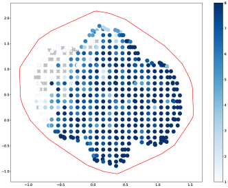
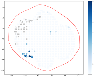
Figure 9: Number of algorithms that found a feasible solution (left), and number of algorithm that found the best-known solution (right). Problem instances for which none of the algorithms found a feasible solution are indicated by a grey x-mark.

As a measure of instance hardness, Figure 9 shows for each instance the number of algorithms that found a feasible solution and those that found the best-known solution. For 51 out of the 518 additional instances and 4 out of the 45 ITC2021 competition instances, no solver found a feasible solution (recall that by design, a feasible solution exists). The figure once more hints that the most difficult problem instances are all situated in the top left corner of the figure. Based on the instance space analysis (see Figure 4), this area is mainly populated by phased problems that have a SE1 soft and a BR2 hard constraint. On the other hand, it seems that at the bottom-left there is a region, characterized by the lack of BR2 constraints and a small number of teams, for which several algorithms find a solution of the same quality.

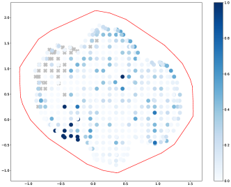
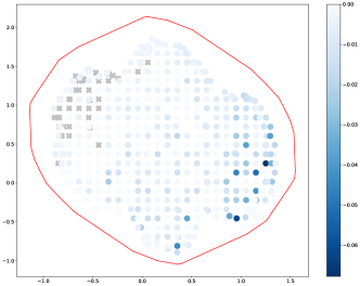
Figure 10: Relative gap with regard to the best solution found over all algorithms and the best lower bound found by MODAL (left), and the detoriation in the relative gap when expressed in terms of the lower bound found at the root node (right). Problem instances for which none of the algorithms found a feasible solution are indicated by a grey x-mark.

Figure 10 compares the best solution found over all algorithms with the best lower bound found by MODAL, using $\text{relative gap}=1-(\text{Best}-\text{LB})/\text{Best}$. The figure reveals that the instances for which multiple algorithms found the same solution can be labeled as ‘easy’, as these solutions turn out to be optimal. For most other instances, considerable improvements in the relative gap are possible. It would be interesting for further research to find out whether this is due to the upper bounds, the lower bounds, or both. In the right of Figure 10, we also show by how much the relative gap deteriorates, when expressed in terms of the lower bound found at the root node. The figure shows that MODAL struggles to improve upon the initial lower bound found when there are fewer BR1 and BR2 soft constraints. This may be a hint that for those problem instances, the IP solvers fail to find clear guidance towards good solutions but rather tend to jump randomly around. The latter was confirmed by analysing the number of better solutions found after a restart of the solver took place.

6 Algorithm selection

Section 4 revealed that there is no single best solver that performs best on all problem instances, and that depending on the location in the instance space, some algorithms may work better than others. This section therefore investigates whether we can develop algorithm selection techniques to predict which algorithm is most suitable for each of the problem instances. Section 6.1 introduces the type of algorithm selection techniques that we consider, Section 6.2 explains how we tuned the parameters of the machine learning techniques and explains the feature selection process. Next, Section 6.3 provides the automated algorithm selection choices, and finally Section 6.4 evaluates the contribution of each algorithm to the algorithm portfolio.

6.1 Algorithm selection techniques

The goal of algorithm selection is to use the properties of problem instances to predict the performance of algorithms on a per-instance level, without actually running the algorithms (see also Rice [28]). Generally speaking, there are two main directions that have been followed by researchers to make these predictions. The first direction is to construct for each algorithm a separate regression model that predicts the quality of the best solution found, and then recommend the algorithm with the highest expected quality (see e.g., De Coster et al [7]). A second option is to directly label each problem instance with the best performing algorithm, and subsequently train a classification algorithm to predict the best performing algorithm (see e.g., de la Rosa-Rivera et al [8]).

In this paper, we ignore all problem instances for which there is no unique best performing algorithm (which are rare, see Figure 9, right). Next, we consider classification as well as regression-based models and evaluate the performance of the machine learning techniques based on the following three metrics.

1. Number of feasible solutions. As many instances pose a significant challenge for algorithms to find even a feasible solution, a first metric is to count the number of feasible solutions found. We denote this metric as $\phi=|\{i\in I:p_{i,c(i)}\neq\leavevmode\hbox to4.2pt{\vbox to4.2pt{\text{[drawing]}}}\}|$, where $i$ is a given instance from the set of test or validation instances $I$, and $c(i)$ is the recommended algorithm.

2. Accuracy. While finding a feasible solution is obviously important, so is the quality of the solutions found. The second metric determines how often the recommended algorithm matches the best performing algorithm: $acc=|\{i\in I:\Delta_{i,c(i)}=0\}|/|I|$.

3. Relative gap. As recommending a near-optimal algorithm is still better than recommending an algorithm that results in a poor or even no solution at all, a second measure is based on the average relative gap: $\bar{\epsilon}=\sum_{\begin{subarray}{c}i\in I:\\ \epsilon_{i,c(i)}\neq\leavevmode\hbox to4.2pt{\vbox to4.2pt{\text{[drawing]}}}\end{subarray}}\epsilon_{i,c(i)}/|I|$.

As in De Coster et al [7], we used the following four different classification algorithms: k-nearest neighbours classification (kNN), random forest classification (RF), gradient-boosted trees (GB), and support vector machines (SVM). In addition, we also consider the regression variants of the above algorithms, where we first trained one regression model for each algorithm predicting the normalized gap of that algorithm, and then select the algorithm with the lowest predicted gap. Finally, we also consider a majority voting classifier (MV) which simply predicts the algorithm that has been predicted most frequently by the machine learning models. All algorithms were implemented using Python’s scikit-learn package.

To train and evaluate the machine learning models, we used a random 80/20 split of the additional problem instances. We refer to the 80% split as the training data, and to the 20% split as the validation data. Although around 500 problem instances is rather limited to learn algorithm performance, we believe that valuable and reliable insights can still be obtained as the problem instances are quite diverse as confirmed by the instance space analysis. Finally, to assess the performance of the machine learning models, we use the original ITC2021 competition instances as the test set.

6.2 Feature selection and parameter configuration

Machine learning algorithms often perform better when not all problem features are used, as this helps to avoid overfitting. For this reason, we performed a recursive feature elimination process using a support vector machine with linear kernel and all other parameters set to their default values. In essence, recursive feature elimination fits a model and then subsequently removes the weakest feature until the desired number of features is reached. We implemented recursive feature selection using scikit-learn’s RFECV package in combination with 10-fold cross-validation on the training data set. The results of the feature selection process are shown in Figure 11.

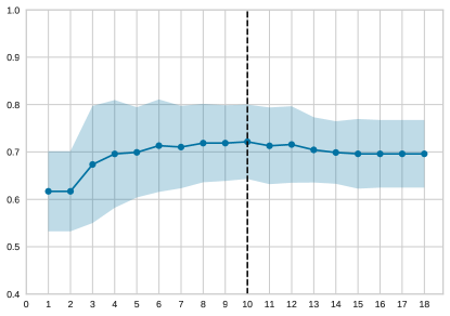
Figure 11: Recursive feature selection showing the number of selected features versus classification accuracy. The model decided to include the following 10 features: $f_{P}$, $f_{|T|}$, $f^{H}_{\text{CA1}}$, $f^{H}_{\text{CA3}}$, $f^{H}_{\text{CA4}}$, $f^{S}_{\text{BR1}}$, $f^{H}_{\text{BR2}}$, $f^{S}_{\text{BR2}}$ , $f^{S}_{\text{FA2}}$, and $f^{S}_{\text{SE1}}$. The shaded area corresponds to one standard deviation above and below the mean accuracy score.

To select the parameters of the machine learning techniques, we performed a complete enumeration of the parameter options (i.e., grid-search) on the training data in combination with ten-fold cross validation using the accuracy metric for the classification models and the score metric for the regression-based models. The final selected parameters for each model are summarized in Table 3.

Classifier	Parameter choice	Parameter choice
kNN	n neighbours$=\{15,[5,25]\}$	Algorithm$=\{ball\_tree,\{brute,$
	Weights$=\{distance,\{uniform,distance\}\}$	Algorithm$=\{$$ball\_tree,kd\_tree\}\}$
SVM	kernel$=\{linear,\{linear,rbf,poly\}\}$	C$=\{1,[0.1,10]\}$
RF	n estimators$=\{200,[10,300]\}$	Max depth$=\{6,[1,8]\}$
GB	n estimators$=\{10,[10,200]\}$	Max depth$=\{4,[2,8]\}$

Table 3: Selected hyperparameters for the machine learning models. The first number between curly brackets gives the parameter value for the classification variant. Next the range of parameter values used for the various the regression variants is given.

6.3 Automated algorithm recommendations

Figure 12 provides an overview of the classification errors made by the majority voting classifier, using the relative gap to represent the degree of misclassification. The figure reveals that the majority voter rarely makes mistakes near the complete left and right of the figure; Figure 6 shows that Udine and FBHS clearly dominate in these regions. On the other hand, more mistakes are made near the middle of the instance space. Though, only for very few misclassifications, this results in a significantly worse relative gap.

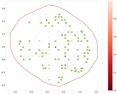
Figure 12: Performance of the majority voting classifier in terms of correctly (green circles) and incorrectly predicted algorithms (red stars) for the validation and test set. The degree of misclassification is quantified by the relative gap of the predicted algorithm, with darker colors indicating more severe errors and treating $\epsilon_{i,c(i)}=\leavevmode\hbox to4.2pt{\vbox to4.2pt{\text{[drawing]}}}$ as zero.

The performance of the machine learning models on the validation and test sets in terms of the number of feasible solutions, accuracy, and relative gap can be seen in the bars on the right side of Figure 13. The bars on the left represent the performance achieved by the individual algorithms, without utilizing any algorithm selection model. Several important insights can be obtained from this figure.

First of all, the figure shows that if only one algorithm can be chosen to solve all problem instances, it is best to select the solver developed by Udine. This strategy not only maximizes the number of feasible solutions found, but also the accuracy and relative gap. The second best choice would be to select the FBHS solver: although the difference in accuracy is small, the relative gap is somewhat less promising which is a consequence from the fact that the FBHS solver finds fewer feasible solutions than Udine. Another interesting observation is that, although UoS and Goal, and to a somewhat lesser extent DITUoIArta, have a significant lower accuracy, their relative gap values are quite similar to that of FBHS. This suggest that these three solvers perform well on most of the problem instances, but are rarely the best performing algorithm.

Second, comparing performance of the machine learning models to the standalone algorithms, it is clear that the former succeed in combining the strengths of different solvers. Indeed, by utilizing machine learning techniques, the accuracy of selecting the best performing algorithm improves by over 30% on the validation set and over 20% on the test set. Additionally, the relative gap is enhanced by about 7% on both the validation and test sets without sacrificing the total number of feasible solutions found. These results are particularly noteworthy since research communities often require years of dedicated research to achieve comparable improvements. Furthermore, the high-level features used in the machine learning models are relatively easy to predict for future problem instances that will be solved by practitioners. Comparing the performance of the machine learning models, the figure hints that the best models consist of the kNN based classifier.

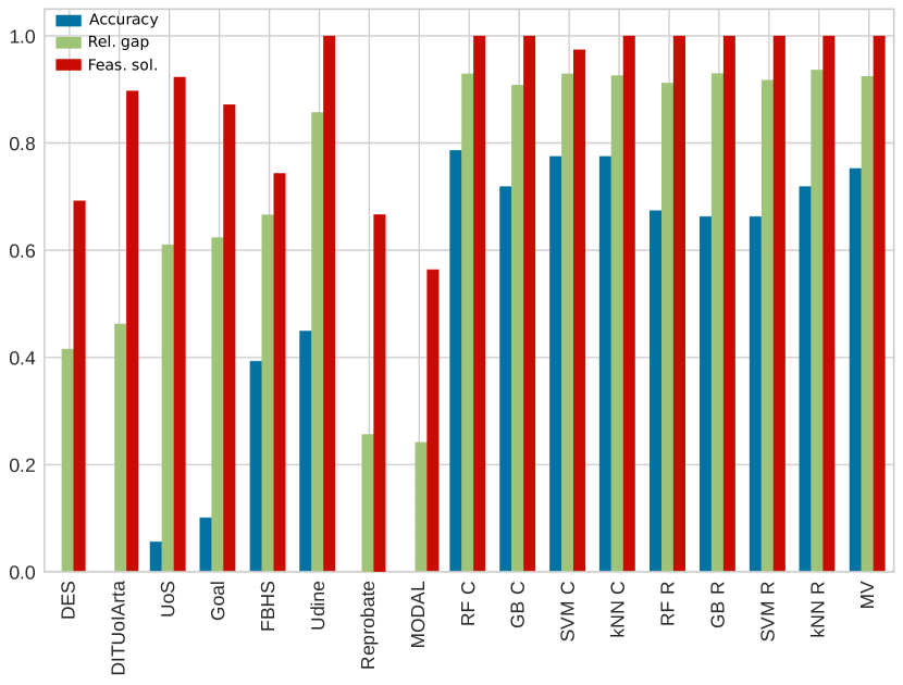
(a) Validation set

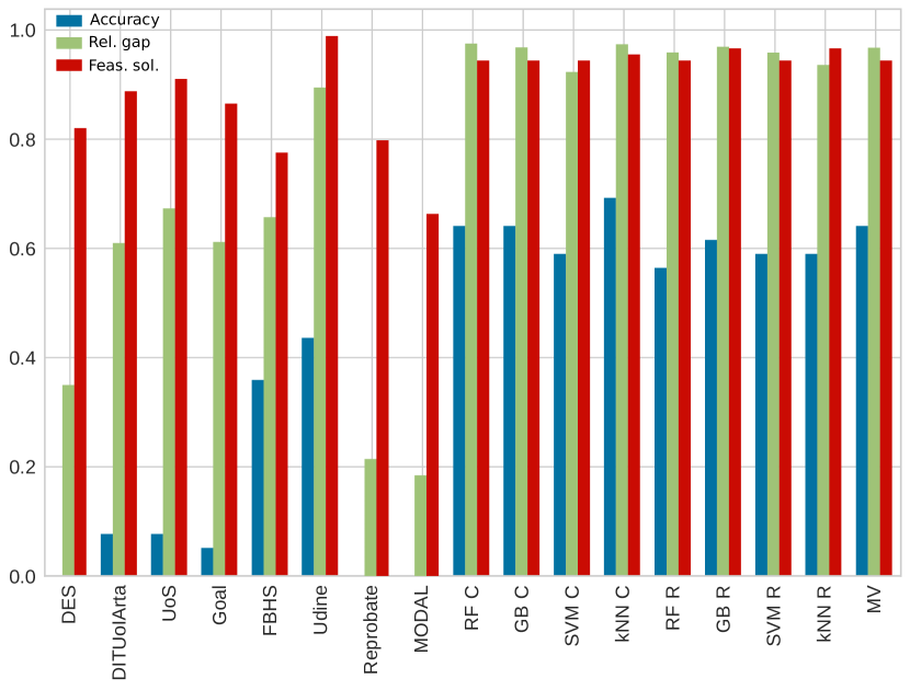
(b) Test set

Figure 13: Evaluation measure results for the different algorithms and classifiers on the validation and test instance set

Finally, in order to understand which features matter to make the predictions, Figure 14 provides estimated feature importances for the predictions of the kNN classifier. These estimates are obtained by randomly permuting the values of a particular feature, effectively disabling this feature, after which the drop in accuracy is computed. This analysis was implemented using the permutation_importance function from scikit’s inspection package. The figure shows that the most indicative features are $f^{S}_{\text{SE1}},f^{S}_{\text{BR2}}$, and $f^{H}_{\text{BR2}}$. Perhaps somewhat unexpected is the importance of the $f^{S}_{\text{SE1}}$ which may be explained by the fact that IP solvers struggle to model this constraint which requires linearisation techniques (see e.g., Berthold et al [4]), while the metaheuristic of Udine deals quite efficiently with this constraint by using a dedicated operator. The negative drop in accuracy for $f^{S}_{\text{BR1}}$ means that the accuracy in fact improves when the $f^{S}_{\text{BR1}}$ values are permuted, but can perhaps best be explained by randomness in the data.

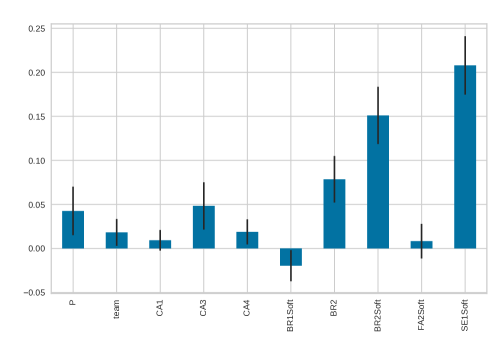
Figure 14: Feature permutation importance based on the kNN classifier, showing for each of the selected features the mean decrease in classification accuracy when disabling the feature.

6.4 Analysis of algorithm complementarity

The previous sections have shown that sports timetabling algorithms have different strengths and weaknesses, allowing machine learning techniques to construct a portfolio of algorithms that together performs better than its individual components. An interesting question is to what extent each of the algorithms contributes to the strength of the portfolio. One possibility to measure an algorithm’s contribution is its standalone performance in terms of the relative gap. However, this metric completely overlooks the complementarity of solvers. For instance, a perfect clone of an algorithm would receive exactly the same score, although clearly not adding much value to the portfolio. A second possibility is to calculate the marginal performance of an algorithm, which is the difference in performance between the portfolio of all algorithms and the portfolio after removing the algorithm. In other words, the marginal performance indicates the improvement in the relative gap when a new algorithm becomes available to an error-free algorithm recommendation system (see, e.g., Wagner et al [40]). Table 4 shows that Udine and FBHS receive the highest marginal score, which is likely due to the fact that Udine provides several solutions to otherwise unsolved problem instances and that FBHS is able to improve upon many solutions. All other solvers receive very low scores, likely due to their strongly correlated performance. Nonetheless, having at least one of these algorithms in the portfolio is desirable and should therefore be rewarded. To that purpose, Table 4 also provides Shapley scores which are equal to the marginal performance of an algorithm with respect to all possible algorithm (sub)portfolios (see Fréchette et al [14]). As Table 4 shows, the strength of the algorithm portfolio not only comes froom Udine and FBHS, but also from the inclusion of DITUoIArta, UoS, and Goal, which on average improve the relative gap of a portfolio by 10 to 15 percentage points.

	DES	DITUoIArta	UoS	Goal	FBHS	Udine	Reprobate	MODAL
Standalone	0.41	0.51	0.64	0.64	0.62	0.87	0.27	0.26
Marginal	0	0	0	0.01	0.10	0.12	0	0
Shapley	0.06	0.09	0.14	0.14	0.21	0.29	0.04	0.04

Table 4: Standalone, marginal, and Shapley scores in terms of the relative gap

7 Conclusion

This study offers an instance space analysis for sports timetabling, resulting in an algorithm selection system that predicts the best algorithm given the high-level features of a problem instance. In a sense, this papers completes the work by [39], which classified the various constraints in sports timetabling and offers a unified problem instance file format, and [37], which set up the ITC2021 timetabling competition leading to the development of the 8 state-of-the-art general sports timetabling solvers that have been used for this paper. The analysis of the algorithm performances on the instance space generated in this paper identifies algorithm strengths and weaknesses, and provides researchers with insights of the most critical features to focus on. Hence, we expect that this study triggers further improvements on the instance benchmark, which can be tracked on itc2021.ugent.be. Indeed, this benchmark remains challenging, knowing that so far only 2 instances have been solved to optimality.

As an area for future work, we like to point out that algorithms in a portfolio can add value beyond the situation where we might select them as the best algorithm to run. At the same time, this serves as a caveat to our analysis of algorithm complementarity. Indeed, if algorithms are usable in conjunction (i.e. the output of one feeding into another, forming a composite algorithm), an individual algorithm could substantially improve the overall performance, even if weak as a standalone. This was demonstrated by the DES algorithm at the conclusion of ITC2021. Warm-starting on the best-known solution for each instance (effectively generated by a portfolio of all other algorithms), it was able to improve a third of these solutions relatively quickly [25]. Likewise, given the complementary performances of the Udine and the FBHS solver, it seems a promising line of research to see whether an hybrid approach, warm starting the Udine solver with the best solution found by the FBHS solver (perhaps ran with a smaller amount of computation time, and possibly violating some of the hard constraints) will lead to further performance improvements for this challenging problem.

In memoriam

We dedicate this article to Jan-Patrick Clarner, who passed away unexpectedly during this research. He wrote his last email about where we could continue his work.

References

- Abdi and Williams [2010] Abdi H, Williams LJ (2010) Principal component analysis. Wiley Interdiscip Rev Comput Stat 2:433–459
- Anagnostopoulos et al [2006] Anagnostopoulos A, Michel L, Van Hentenryck P, Vergados Y (2006) A simulated annealing approach to the traveling tournament problem. J Sched 9:177–193
- Berthold et al [2019] Berthold T, Lodi A, Salvagnin D (2019) Ten years of feasibility pump, and counting. EURO Journal on Computational Optimization 7:1–14
- Berthold et al [2021] Berthold T, Koch T, Shinano Y (2021) MILP. Try. Repeat. In: De Causmaecker P, Özcan E, Vanden Berghe G (eds) Proc. 13th Int. Conf. Pract. Theory Autom. Timetabling, PATAT, vol 2, pp 403–411
- Briskorn [2008] Briskorn D (2008) Feasibility of home-away-pattern sets for round robin tournaments. Oper Res Lett 36:283 – 284
- Ceschia et al [2023] Ceschia S, Di Gaspero L, Schaerf A (2023) Educational timetabling: Problems, benchmarks, and state-of-the-art results. Eur J Oper Res 308:1–28
- De Coster et al [2022] De Coster A, Musliu N, Schaerf A, Schoisswohl J, Smith-Miles K (2022) Algorithm selection and instance space analysis for curriculum-based course timetabling. J Sched 25
- de la Rosa-Rivera et al [2021] de la Rosa-Rivera F, Nunez-Varela JI, Ortiz-Bayliss JC, Terashima-Marín H (2021) Algorithm selection for solving educational timetabling problems. Expert Syst Appl 174:114694
- Dimitsas et al [2022] Dimitsas A, Gogos C, Valouxis C, Tzallas A, Alefragis P (2022) A pragmatic approach for solving the sports scheduling problem. In: Proc. 13th Int. Conf. Pract. Theory Autom. Timetabling, PATAT, vol 3, pp 195–207
- Durán et al [2021] Durán G, Gutiérrez F, Guajardo M, Marenco J, Sauré D, Zamorano G (2021) Scheduling the main professional football league of Argentina. INFORMS Journal on Applied Analytics 51:361–372
- Easton et al [2001] Easton K, Nemhauser G, Trick M (2001) The traveling tournament problem description and benchmarks. In: Walsh T (ed) Principles and Practice of Constraint Programming — CP 2001, Springer, Berlin, Heidelberg, pp 580–584
- Elffers and Nordström [2018] Elffers J, Nordström J (2018) Divide and conquer: Towards faster pseudo-boolean solving. In: Lang J (ed) Proceedings of the Twenty-Seventh International Joint Conference on Artificial Intelligence, IJCAI 2018, July 13-19, 2018, Stockholm, Sweden, ijcai.org, pp 1291–1299
- Fonseca and Toffolo [2022] Fonseca GHG, Toffolo TAM (2022) A fix-and-optimize heuristic for the ITC2021 sports timetabling problem. J Sched 25:273–286
- Fréchette et al [2016] Fréchette A, Kotthoff L, Michalak T, Rahwan T, Hoos HH, Leyton-Brown K (2016) Using the shapley value to analyze algorithm portfolios. In: Proc. of the Thirtieth AAAI Conference on Artificial Intelligence, AAAI Press, AAAI’16, pp 3397–3403
- Gebser et al [2007] Gebser M, Kaufmann B, Neumann A, Schaub T (2007) clasp : A conflict-driven answer set solver. In: Baral C, Brewka G, Schlipf JS (eds) Logic Programming and Nonmonotonic Reasoning, 9th International Conference, LPNMR 2007, Tempe, AZ, USA, May 15-17, 2007, Proceedings, Springer, Lecture Notes in Computer Science, vol 4483, pp 260–265
- Goossens and Spieksma [2009] Goossens D, Spieksma F (2009) Scheduling the Belgian soccer league. Interfaces 39:109–118
- Januario and Urrutia [2016] Januario T, Urrutia S (2016) A new neighborhood structure for round robin scheduling problems. Computers & Operations Research 70:127–139
- Johnson et al [1989] Johnson DS, Aragon CR, McGeoch LA, Schevon C (1989) Optimization by simulated annealing: An experimental evaluation; part I, graph partitioning. Operations research 37:865–892
- Kerschke et al [2019] Kerschke P, Hoos HH, Neumann F, Trautmann H (2019) Automated algorithm selection: Survey and perspectives. Evol Comput 27:3–45, pMID: 30475672
- Kletzander et al [2021] Kletzander L, Musliu N, Smith-Miles K (2021) Instance space analysis for a personnel scheduling problem. Annals of Mathematics and Artificial Intelligence 89:617–637
- Lamas-Fernandez et al [2021] Lamas-Fernandez C, Martinez-Sykora A, Potts CN (2021) Scheduling double round-robin sports tournaments. In: De Causmaecker P, Özcan E, Vanden Berghe G (eds) Proc. 13th Int. Conf. Pract. Theory Autom. Timetabling, PATAT, vol 2, pp 435 – 448
- Le Berre and Wallon [2021] Le Berre D, Wallon R (2021) On dedicated CDCL strategies for PB solvers. In: Li C, Manyà F (eds) Theory and Applications of Satisfiability Testing - SAT 2021 - 24th International Conference, Barcelona, Spain, July 5-9, 2021, Proceedings, Springer, Lecture Notes in Computer Science, vol 12831, pp 315–331
- Lester [2022] Lester MM (2022) Pseudo-boolean optimisation for robinx sports timetabling. J Sched 25:287–299
- Nemhauser and Trick [1998] Nemhauser GL, Trick MA (1998) Scheduling a major college basketball conference. Oper Res 46:1–8
- Phillips et al [2021] Phillips AE, O’Sullivan M, Walker C (2021) An adaptive large neighbourhood search matheuristic for the ITC2021 sports timetabling competition. In: De Causmaecker P, Özcan E, Vanden Berghe G (eds) Proc. 13th Int. Conf. Pract. Theory Autom. Timetabling, PATAT, vol 2, pp 426 – 430
- Recalde et al [2013] Recalde D, Torres R, Vaca P (2013) Scheduling the professional Ecuadorian football league by integer programming. Comput Oper Res 40:2478 – 2484
- Ribeiro and Urrutia [2012] Ribeiro CC, Urrutia S (2012) Scheduling the Brazilian soccer tournament: Solution approach and practice. INFORMS Journal on Applied Analytics 42:260–272
- Rice [1976] Rice JR (1976) The algorithm selection problem. Adv Comput 15:65–118
- de la Rosa-Rivera et al [2021] de la Rosa-Rivera F, Nunez-Varela JI, Puente-Montejano CA, Nava-Muñoz SE (2021) Measuring the complexity of university timetabling instances. Journal of Scheduling 24:103–121
- Rosati et al [2022] Rosati RM, Petris M, Di Gaspero L, Schaerf A (2022) Multi-neighborhood simulated annealing for the sports timetabling competition ITC2021. J Sched 25:301–319
- Smith-Miles and Bowly [2015] Smith-Miles K, Bowly S (2015) Generating new test instances by evolving in instance space. Comput Oper Res 63:102–113
- Smith-Miles and Lopes [2012] Smith-Miles K, Lopes L (2012) Measuring instance difficulty for combinatorial optimization problems. Comput Oper Res 39:875 – 889
- Smith-Miles et al [2014] Smith-Miles K, Baatar D, Wreford B, Lewis R (2014) Towards objective measures of algorithm performance across instance space. Comput Oper Res 45:12 – 24
- Sutton and Barto [2018] Sutton RS, Barto AG (2018) Reinforcement learning: An introduction. MIT press
- Trick [2001] Trick MA (2001) A schedule-then-break approach to sports timetabling. In: Burke E, Erben W (eds) Pract. Theory Autom. Timetabling III, Springer, Berlin, Heidelberg, pp 242–253
- Van Bulck and Goossens [2023] Van Bulck D, Goossens D (2023) First-break-heuristically-schedule: Constructing highly-constrained sports timetables. Operations Research Letters 51:326–331
- Van Bulck and Goossens [2023] Van Bulck D, Goossens D (2023) The international timetabling competition on sports timetabling (ITC2021). Eur J Oper Res 308:1249–1267
- Van Bulck et al [2019] Van Bulck D, Goossens DR, Spieksma FCR (2019) Scheduling a non-professional indoor football league: a tabu search based approach. Ann Oper Res 275:715–730
- Van Bulck et al [2020] Van Bulck D, Goossens D, Schönberger J, Guajardo M (2020) RobinX: A three-field classification and unified data format for round-robin sports timetabling. Eur J Oper Res 280:568 – 580
- Wagner et al [2018] Wagner M, Lindauer M, Mısır M, Nallaperuma S, Hutter F (2018) A case study of algorithm selection for the traveling thief problem. Journal of Heuristics 24:295–320
- de Werra [1981] de Werra D (1981) Scheduling in sports. In: Hansen P (ed) Studies on graphs and discrete programming, North-Holland, Amsterdam, pp 381–395
- Westphal [2014] Westphal S (2014) Scheduling the German basketball league. Interfaces 44:498–508