1 Introduction

Motivation.

Arguably, the most impactful realization in early last-century quantitative sciences was the combination of the loose notions of symmetry with the precise definition of algebraic groups. From important results in cryptography [40], passing through the description of the hydrogen atom [91] and the standard model of particles [41], arriving at the formalization of Klein’s Erlanger program [30], the group-theoretic point of view on symmetries allowed for unprecedented developments in many theoretical and practical fields. Therefore, it is unsurprising that the prominent role assumed by symmetries translated itself to the description of learning, be it natural—e.g., the detection of invariances in visual psychology [48, 47]—or artificial. Indeed, the ability to identify that a rotated ‘7’-digit is still a 7 tells us much about the important presence of symmetries—and, consequently, of groups—in the process of ‘understanding’.

Notice that the symmetries are not restricted to the cognition part of the process—i.e., they are not only devices created by our brain to simplify its training task, although they can be, sometimes, artificially-induced—, but they are inherited from the learning data. It is because we have seen many images of the same object rotated around its center or shifted in space and have been told, in whatever form, that these correspond to the same entity, that we acquired the invariance of the digit ‘7’ with respect to rotations. In a nutshell, this indicates that there is a genuine interest to identify, directly from data, the existence of symmetries on it, something which we review below. Whether and how the information of existing symmetries is used to improve the training process (which it does, as, again, we will review) is not the focus here; rather, we are primarily interested in the ability to tell, from data only, the existence of groups symmetries, their specifications, and the ‘symmetry’ types. Although not the focus, we give some taste of how this knowledge can improve Machine Learning algorithms in Section 6.

We attempt to tackle the symmetry identification problem algorithmically. That is, in a more mathematical language, our goal is to create a technique to determine the actions of groups that generate the symmetries on a data set. Of course, as stated, this task is rather open, so we assume some constraints. The first of these is related to the algebraic groups considered. Instead of an algorithm that works for the whole class of groups, we will focus on detecting symmetries generated by Lie groups, those admitting smooth structures within their operations. In fact, the set of all Lie groups is still too big, so we will concentrate only on compact Lie groups, for reasons that will become clear throughout the text.

We will also restrict the kinds of symmetry, or in group language, actions, that describe how the Lie groups interact with datasets. Instead of the general scenario, we consider only representations, which are linear actions of Lie groups in vector spaces. This means that only one particular kind of data set, the point clouds living in some $\mathbb{R}^{n}$, will be of any interest to us. More precisely, we study point clouds $X$ that are sampled on or close to a submanifold $\mathcal{O}$ that carry a transitive action of its symmetry group. Equivalently, $\mathcal{O}$ is the orbit of a compact Lie group representation. Moreover, it is always possible to embed such Lie groups symmetries as $n\times n$ matrices, which significantly simplifies the computations performed.

Although unapologetically restrictive compared to the general problem of determining arbitrary actions of arbitrary groups on arbitrary data sets, the constrained setting of representations of compact Lie groups in point clouds still sets the stage for many interesting problems in data science, some of which we motivate in the examples below, further explored in Section 6.

Example 1.1 (Pixel permutations, Section 6.1).

Consider a set of $m_{x}\times m_{y}$-pixeled images such that each of them is generated by a simple permutation of the pixels of another fixed image. Supposing these permutations form a finite group $\Sigma$, then the embedding of the images in $\mathbb{R}^{m_{x}\times m_{y}}$ will necessarily lie on a representation orbit of $\Sigma$ in $\mathbb{R}^{m_{x}\times m_{y}}$. As it turns out, when $\Sigma$ is Abelian, the data also lies on an orbit of the compact Lie group $T^{d}$, the $d$-dimensional torus, which may then be used to reconstruct the group from the embedded vectors only.

Example 1.2 (Harmonic analysis, Section 6.2).

Abstract harmonic analysis is often referred to as the study of signal decomposition in arbitrary groups. For the case of compact Lie groups, the existence of a discrete orthonormal basis for the set of $L^{2}$-integrable functions is guaranteed by the Peter-Weyl theorem, which implies that such a basis is parametrized by $\widehat{G}$, the complex irreducible representations of $G$. In particular, ordinary harmonic analysis, taken as the decomposition of periodic functions through sines and cosines, is but a special case of this result. Suppose then $\{(x_{i},y_{i})\}_{i=1}^{N}$ is a data set, where each $x_{i}$ lies in the orbit $\mathcal{O}$ of a representation of a compact Lie group $G$, $y_{i}$ are real scalars, and there is an unknown function $f:\mathcal{O}\to\mathbb{R}$ such that $f(x_{i})\approx y_{i}$. If $\{f_{[\phi]}\}_{[\phi]\in\hat{G}}$ is an abstract harmonic analysis basis for $G$, then this regression can be written as

$$f=\sum_{[\phi]\in\widehat{G}}a_{[\phi]}f_{[\phi]},$$

where $a_{[\phi]}$ are complex constants. Not only does the summation above converge in the whole function’s domain, but the functions $f_{[\phi]}$ can be known for every choice of $G$. Therefore, the knowledge that the input data lies close to an orbit of a compact Lie group $G$ suggests a linear regression solution to the machine learning problem.

Example 1.3 (Hamiltonian systems, Section 6.3).

The fundamental role of Lie groups in modern Physics, especially in its more mathematical formulation, was initially identified by the Noether theorem, which established the well-known one-to-one correspondence between actions of Lie groups and conserved variables in classical mechanics [69]. The following decades, however, not only expanded this correspondence to many other areas of Physics—from general relativity to quantum field theory—but was used for solving several classical problems [91]. Due to its more geometric formulation, Hamiltonian mechanics is particularly susceptible to receiving treatment through Lie theory in determining conserved observables, allowing for the direct derivation of constants of motion from the knowledge of Lie action orbits.

Our contribution and related work.

In Algorithm 3.1, we propose a framework to transform the problems from the last examples in machine learning tasks. The precise model assumed will be formalized in Section 3, but simply put, we take a representation $\phi:G\to\mathrm{GL}_{n}(\mathbb{R})$ of a compact Lie group $G$ in some vector space $\mathbb{R}^{n}$, for which $\mathcal{O}\subseteq\mathbb{R}^{n}$ is one of its orbits. We want to determine $\phi$ using only a point cloud $X$ well enough sampled in $\mathcal{O}$. Moreover, because the knowledge of $\phi$ permits the reconstruction $\mathcal{O}$, it is possible to determine which of the compact Lie groups is most likely to have generated the orbit. Unfortunately, this is an ill-posed problem: two distinct compact Lie groups can generate the same orbit $\mathcal{O}$; moreover, fixed a compact Lie group $G$, two of its distinct representations can also generate $\mathcal{O}$. Ignoring these subtleties for now, we stress that, as far as we know, ours is the first reported technique in literature to identify both the precise representation type and the most likely acting Lie group. We believe that such information may be fruitful in developing new inference techniques and application settings, some of which we already suggest here. Besides, the theoretical guarantees of Section 5 already imply strong robustness results to our algorithm, which is seen to work even when available data $X$ does not sit perfectly within $\mathcal{O}$.

On the other hand, although new in its precise structure, our approach is not the first attempt to solve this sort of problem, given the long history of interest in action detection problems. For example, as indicated by [78], the related problem of symmetry identification has been tackled since the 1980s, with algorithms for symmetries of $\text{SE}(2)$ representations in planar data [92, 44]. A similar task, now for 3D objects, was often addressed in the literature, as well-reviewed by [66]. We stress, however, that all these works are limited to the detection of symmetries as subgroups of known groups, a scope much more restricted than ours.

The above limitation was addressed by some research aimed at automatically detecting the representation operators of more general Lie groups from different data sets. Sohl-Dickstein, Wand, and Olshausen, for example, use a modified version of the MAP algorithm to estimate the operators $T$ such that $\sum_{t}|x^{(t)}-Tx^{(t-1)}|$ is minimized [80]. Although having the obvious advantage of dealing with naturally sequential data—the paper consider applications of this method to videos, for example—the technique is not general enough to consider arbitrary commutation of group elements, being perhaps better suited to Abelian Lie groups. Cohen and Welling, once more, also address the problem of determining the exact representation operators from the orbit points using a Bayesian approach; however, besides being restricted only to Abelian Lie groups, they do not try to project the operators into the closest Lie algebra, meaning that no information about the exact representation type is retrieved [20]. A more recent approach, now useful even for orbits of non-Abelian Lie groups, was introduced by [73] in response to the problem raised by [43] which, using methods from Riemannian geometry, estimates local basis for orbits of direct products of Lie groups.

In [26], on the other hand, the authors use a generalization of the $G$-CNN architecture, now to Lie algebras convolutions, to estimate derived representation operators, denoted $X$, in data sets for supervised tasks that are equivariant under some unknown Lie group $G$. Although similar to our work, this approach not only again gives the Lie algebra operators only as a vector space—i.e., there is no attempt to project the estimated $X$ onto the closest derived representation of $G$—but the output may also be an over-determined set of vector, meaning that it does not even form a basis for the Lie algebra of $G$. This issue is resolved by Cahill et al. in [15], where the exact Lie algebra of the symmetry group of the orbit, denoted by $\mathfrak{sym}(\mathcal{O})$, seen only as a vector space, is estimated, together with its dimension, through spectral decomposition of an operator. Our algorithm is, in fact, a generalization of this last work, where instead of only finding the basis for $\mathfrak{sym}(\mathcal{O})$ we project it into the closest representation of the associated Lie group. Moreover, while the approach by Cahill et al. permits an estimation of the symmetry group only, our generalization allows for estimating the representation of different Lie groups which also have actions in the embedding space of orbit $\mathcal{O}$.

Once the information of acting Lie groups is determined, it can be used to increase the efficiency of other inference and machine learning tasks. In this context, the interest often lies in devising equivariant algorithms, that is, maps $\Phi:X\to Y$ from the input to the output spaces such that, for a fixed group $G$ with actions on $\cdot_{X}$ and $\cdot_{Y}$ in $X$ and $Y$, we have $\Phi(g\cdot_{X}X)=g\cdot_{Y}\Phi(X)$ for all $g\in G$. In particular, already in 1995, LeCun et al. showed that convolution neural networks [58], introduced by some of the same authors in 1989, have all their convolution and pooling layers equivariant under translations in the pixel grid [57]. Nevertheless, it was only in 2016 that Cohen and Welling extended this architecture to general group actions [21], achieving the state-of-the-art at the time for the rotated MNIST data set [56] through employing finite groups. These equivariant networks for pixel data were later expanded to Lie group actions in works such as [94, 55, 27, 18, 8, 32, 93, 90], where equivariance under the usual $\text{SE}(2)=\mathrm{SO}(2)\times\mathbb{R}^{2}$ representation in the plane is guaranteed using different techniques and then applied to problems ranging from microscopic imaging to galaxy morphology classification. Solutions to pixel data in $\mathbb{R}^{3}$, here equivariant under the natural $\mathrm{SO}(3)$ representations, were developed [22]. Similar $G$-CNN architectures were suggested for problems equivariant under representations of $\text{SE}(3)$ [38, 37, 83] to dynamical systems conservation laws [32], and the Lorentz group, responsible for describing relativistic particles behavior [11]. Finally, Finzi, Welling, and Wilson suggested a general automatic technique for achieving equivariant architectures for any Lie group representation [33]. In contrast, Kondor and Trivedi showed that, under minor assumptions, $G$-CNN implementations are the only feed-forward neural network architectures equivariant for compact Lie group representations [54].

Technical aspects.

In addition to applications, this article places particular emphasis on theoretical justification. As far as geometry is concerned, we follow standard ideas of the literature regarding manifold and tangent space estimation, involving notions of geometric measure theory [1, 12]. In particular, we adopt a measure-theoretic point of view of the problem. This is part of a movement in recent research to express stability results with the Wasserstein distance, instead of the traditional Hausdorff distance, less suited to the case of noisy data sets [14, 60, 85]. On the algebraic side, at the core of our algorithm lies Lie-PCA, a recent method for estimating the Lie algebra of symmetry groups [15]. We analyze it by invoking traditional tools of representation theory. Last, regarding implementations, we raise concrete matrix computation problems, such as simultaneous reduction [76, 89, 70, 63] and local PCA [88, 52, 1, 79, 15]. Throughout this paper, and although we do not enter into further details, we draw connections with problems of other areas of mathematics, such as varieties of Lie algebras [36, 74, 62, 6, 3, 86], Linnik type problems [61, 29, 28, 75, 49], and rigidity of Lie subalgebras [5, 4, 23, 7].

Code availability.

We developed a Python library, LieDetect, which fully implements the algorithm described in this paper. This can be found at https://github.com/HLovisiEnnes/LieDetect, together with our experiments from Section 6. In addition, some video animations, illustrating the minimization program performed during the algorithm, are gathered at https://www.youtube.com/playlist?list=PL_FkltNTtklBQlwrGyAnisJ-lGiLFeTVw.

Outline.

The rest of the paper is as follows. In Section 2, we give a self-contained introduction to the theory of representations of Lie groups. We define the main algorithm of this paper in Section 3 and give additional comments regarding its implementation in Section 4. We prove consistency and stability results for the algorithm in Section 5. In Section 6 we apply the algorithm to three concrete machine learning problems. Notations are listed in Appendix A.1, and a few supplementary results are gathered in Appendix A.2.

2 Preliminaries

We now lay the theoretical background needed to read this paper. The first two sections introduce basic notions regarding Lie groups and their representations, following [13]. The third section is dedicated to defining and analyzing the structure of the Stiefel and Grassmann varieties of Lie algebras, which will play a crucial role in our algorithm.

2.1 Lie groups and Lie algebras

2.1.1  Lie groups

A Lie group is a group $G$ that is also a smooth manifold, and such that the multiplication map $(g,h)\mapsto gh$ and the inverse map $g\mapsto g^{-1}$ are smooth. An example is given by the general linear group $\mathrm{GL}_{n}(\mathbb{R})$ of real invertible $n\times n$ matrices, and its complex equivalent $\mathrm{GL}_{n}(\mathbb{C})$. Endowed with the subspace topology inherited from the vector space of $n\times n$ matrices $\mathrm{M}_{n}(\mathbb{R})$ and $\mathrm{M}_{n}(\mathbb{C})$, both $\mathrm{GL}_{n}(\mathbb{R})$ and $\mathrm{GL}_{n}(\mathbb{C})$ are smooth submanifolds, and also Lie groups. They have real dimensions $n^{2}$ and $2n^{2}$, respectively, and are not compact. In what follows, we will focus on compact Lie groups, and more particularly on the orthogonal group $\mathrm{O}(n)$, the special orthogonal group $\mathrm{SO}(n)$, the unitary group $\mathrm{U}(n)$, the special unitary group $\mathrm{SU}(n)$, and the torus $T^{n}$, respectively defined for any integer $n\geq 1$ as:

$$\mathrm{O}(n) =\big{\{}A\in\mathrm{GL}_{n}(\mathbb{R})\mid A^{\top}=A^{-1}\big{\}},$$

$$\mathrm{SO}(n) =\big{\{}A\in\mathrm{GL}_{n}(\mathbb{R})\mid A^{\top}=A^{-1},\det(A)=1\big{\}},$$

$$\mathrm{U}(n) =\big{\{}A\in\mathrm{GL}_{n}(\mathbb{C})\mid A^{*}=A^{-1}\big{\}},$$

$$\mathrm{SU}(n) =\big{\{}A\in\mathrm{GL}_{n}(\mathbb{C})\mid A^{*}=A^{-1},\det(A)=1\big{\}},$$

$$T^{n} =\mathrm{SO}(2)\times\cdots\times\mathrm{SO}(2)~{}~{}~{}~{}\text{(}n\text{ copies)},$$

where $A^{\top}$ denote the transpose and $A^{*}$ the conjugate transpose. These groups have respective dimensions $n(n-1)/2$, $n(n-1)/2$, $n^{2}$, $n^{2}-1$ and $n$, and are all connected, expect for $\mathrm{O}(n)$ which consists of two connected components. Moreover, they are all matrix groups, that is, they can be described as subgroups of a general linear group $\mathrm{GL}_{n}(\mathbb{R})$ or $\mathrm{GL}_{n}(\mathbb{C})$. In general, it is a consequence of Peter–Weyl theorem that any compact Lie group is a matrix group.

A Lie group homomorphism is a smooth group homomorphism between two Lie groups. For instance, embedding $\mathrm{M}_{n}(\mathbb{R})$ into $\mathrm{M}_{n}(\mathbb{C})$ and $\mathrm{M}_{n}(\mathbb{C})$ into $\mathrm{M}_{2n}(\mathbb{R})$ yield Lie group homomorphisms $\mathrm{SO}(n)\hookrightarrow\mathrm{SU}(n)\hookrightarrow\mathrm{SO}(2n)$. If a Lie group homomorphism is bijective with smooth inverse, it is called a Lie group isomorphism, and the Lie groups are said isomorphic. In the list above, all the groups are non-isomorphic, except for $\mathrm{SO}(1)\simeq\mathrm{SU}(1)$, both singletons, and $\mathrm{SO}(2)\simeq\mathrm{U}(1)\simeq T^{1}$. Moreover, any Abelian Lie group of dimension $d$ is isomorphic to $T^{d}$.

It is worth mentioning that being a Lie group imposes strong regularities on the underlying manifold. For instance, they are all orientable. Moreover, the fundamental group of a connected Lie group is discrete and Abelian. As another example, the $n$-sphere $S^{n}$ admits a Lie group structure only when $n=0$, $1$ or $3$, these cases corresponding respectively to the singleton, $\mathrm{SO}(2)$ and $\mathrm{SU}(2)$. Besides, being a Lie group implies the existence of a Lie algebra structure on the tangent spaces, as we review now.

2.1.2  Lie algebras

A Lie algebra is a vector space $V$, together with an operation $[\cdot,\cdot]\colon V\times V\to V$, called Lie bracket, that is bilinear, anti-symmetric, and obeys Jacobi’s identity, that is, $[x,[y,z]]+[y,[z,x]]+[z,[x,y]]=0$ for all $x,y,z\in V$. If $[A,B]=0$ for all $A,B\in V$, then the Lie algebra is said Abelian. By fixing a basis $\{A_{i}\}_{i=1}^{m}$ of the vector space $V$, the structure constants of the Lie algebra relative to this basis are defined as the scalars $\{c_{i,j}^{k}\}_{i,j,k=1}^{m}$ satisfying $[A_{i},A_{j}]=\sum_{k=1}^{m}c_{i,j}^{k}A_{k}$ for all $i,j\in[1\dots m]$. As a particular case, the structure constants of an Abelian Lie algebra are all zero and hence do not depend on the basis. As another example, one defines a Lie bracket on the space of $n\times n$ matrices $\mathrm{M}_{n}(\mathbb{R})$ via the commutator $[A,B]=AB-BA$. This Lie algebra is non-Abelian when $n\geq 2$.

Given a Lie group $G$, its tangent space $\mathrm{T}_{e}G$ at the origin can be canonically endowed with a Lie bracket, yielding a Lie algebra, denoted $\mathfrak{g}$. This construction is commonly based on left-invariant vector fields on $G$, which we do not describe here. When $G\subset\mathrm{M}_{n}(\mathbb{R})$ is a matrix group, a more direct definition exists: the tangent space $\mathrm{T}_{e}G$, seen as a linear subspace of $\mathrm{M}_{n}(\mathbb{R})$, is endowed with the Lie bracket of commutator of matrices. By convention, we write in gothic font the Lie algebra. For instance, the tangent spaces of the general linear group, the special orthogonal group, the special unitary group, and the torus are

$$\mathfrak{gl}(n) =\mathrm{M}_{n}(\mathbb{R}),$$

$$\mathfrak{so}(n) =\{A\in\mathrm{M}_{n}(\mathbb{R})\mid A^{\top}=-A\},$$

$$\mathfrak{su}(n) =\{A\in\mathrm{M}_{n}(\mathbb{C})\mid A^{*}=-A,~{}\mathrm{tr}(A)=0\},$$

$$\mathfrak{t}^{n} =\mathfrak{so}(2)\times\cdots\times\mathfrak{so}(2)~{}~{}~{}\text{(}n\text{ copies)},$$

i.e., $\mathfrak{so}(n)$ is the set of skew-symmetric matrices and $\mathfrak{su}(n)$ of zero-trace skew-Hermitian matrices.

A Lie algebra homomorphism between two Lie algebras $V$ and $W$ is a linear map $\phi\colon V\rightarrow W$ such that $[\phi(A),\phi(B)]=\phi([A,B])$ for all $A,B\in V$. If $\phi$ is bijective, it is called an isomorphism of Lie algebras, and the Lie algebras are said isomorphic. Equivalently, two Lie algebras are isomorphic if they admit the same structure constants in a certain pair of bases. For instance, as shown in the example below, $\mathfrak{su}(2)$ and $\mathfrak{so}(3)$ are isomorphic, although $\mathrm{SU}(2)$ and $\mathrm{SO}(3)$ are not. This shows that the Lie algebra does not totally determine a Lie group. Despite that fact, it contains valuable information about the group, as we explain in the next section.

Example 2.1.

A usual choice of basis for $\mathfrak{so}(3)$, as presented in [30], is

$$X_{1}=\begin{pmatrix}0&0&0\\ 0&0&-1\\ 0&1&0\end{pmatrix},~{}~{}X_{2}=\begin{pmatrix}0&0&1\\ 0&0&0\\ -1&0&0\end{pmatrix},~{}~{}X_{3}=\begin{pmatrix}0&-1&0\\ 1&0&0\\ 0&0&0\end{pmatrix},$$

for which we have the brackets $[X_{1},X_{2}]=X_{3}$, $[X_{2},X_{3}]=X_{1}$ and $[X_{1},X_{3}]=-X_{2}$. Besides, a basis of $\mathfrak{su}(2)$ is given by the Pauli matrices, which yield the same Lie brackets:

$$Y_{1}=\frac{1}{2}\begin{pmatrix}0&i\\ i&0\end{pmatrix},~{}~{}Y_{2}=\frac{1}{2}\begin{pmatrix}0&-1\\ 1&0\end{pmatrix},~{}~{}Y_{3}=\frac{1}{2}\begin{pmatrix}i&0\\ 0&-i\end{pmatrix}.$$

Example 2.2.

It is known that any matrix in $\mathrm{SO}(2)$ can be written as $R(\theta)$ for some $\theta\in[0,2\pi)$, and any matrix in $\mathfrak{so}(2)$ as $L(a)$ for some $a\in\mathbb{R}$, where

$$R(\theta)=\begin{pmatrix}\cos\theta&-\sin\theta\\ \sin\theta&\cos\theta\end{pmatrix}~{}~{}~{}~{}~{}\mathrm{and}~{}~{}~{}~{}~{}L(a)=\begin{pmatrix}0&-a\\ a&0\end{pmatrix}.$$

Consequently, matrices of $T^{d}$ can be written as $\mathrm{diag}(R(\theta_{1}),\dots,R(\theta_{d}))$ for some $(\theta_{1},\dots,\theta_{d})\in[0,2\pi)^{d}$, and matrices of $\mathfrak{t}^{d}$ as $\mathrm{diag}(L(a_{1}),\dots,L(a_{d}))$ for some $(a_{1},\dots,a_{d})\in\mathbb{R}^{d}$.

2.1.3  The exponential map

Given a Lie group $G$ with Lie algebra $\mathfrak{g}$, there exists a canonical smooth map $\exp\colon\mathfrak{g}\rightarrow G$, called the exponential map. In the general construction, it is defined using one-parameter subgroups generated by left-invariant vector fields. In the particular case of matrix groups $G\subset\mathrm{GL}_{n}(\mathbb{R})$, the exponential map is simply the restriction to $\mathfrak{g}$ of the matrix exponential, $\exp\colon\mathrm{M}_{n}(\mathbb{R})\rightarrow\mathrm{GL}_{n}(\mathbb{R})$, defined as $\exp(A)=\sum_{i=0}^{+\infty}A^{n}/n!$. For $A,B\in\mathfrak{g}$, it holds

$$\exp(A+B)=\exp(A)\exp(B)\iff[A,B]=0.$$

Endowing $\mathfrak{g}$ with the group structure of the addition, we deduce that $\exp\colon\mathfrak{g}\rightarrow G$ is a group homomorphism only when $\mathfrak{g}$ is an Abelian Lie algebra, that is, when $G$ is a torus, in the compact case. Moreover, if $G$ is connected and compact or is the general linear group, then the exponential map is subjective. For instance, elements of $\mathrm{SO}(2)$ take the form $R(\theta)$ for some $\theta\in\mathbb{R}$, which in turn is equal to the exponential of $L(\theta)$, defined in Example 2.2.

The exponential map is a fundamental tool in the study of Lie groups, allowing a dialogue between the group and its algebra. To illustrate this phenomenon, any Lie group homomorphism $\phi\colon G\to H$ induces a unique Lie algebra homomorphism $\mathrm{d}\phi\colon\mathfrak{g}\to\mathfrak{h}$ with commutative diagram

(1)

The map $\mathrm{d}\phi$ is called the derived homomorphism of $\phi$, and $\mathrm{d}\phi(\mathfrak{g})\subset\mathfrak{h}$ the pushforward Lie algebra. If $\phi$ is an isomorphism, or surjective with discrete kernel, then $\mathrm{d}\phi$ is an isomorphism. For instance, the well-known double cover $\mathrm{SU}(2)\rightarrow\mathrm{SO}(3)$ yields an isomorphism $\mathfrak{su}(2)\rightarrow\mathfrak{so}(3)$.

In Riemannian geometry, there is a concurrent notion of exponential map. Without entering into the details, we mention that any compact Lie group admits a bi-invariant Riemannian metric. In this case, the Riemannian exponential coincides with the (Lie) exponential [65]. On simple Lie groups, such as $\mathrm{SO}(n)$ with $n\neq 4$, such a metric is unique up to a constant.

The Frobenius inner product $\langle A,B\rangle=\operatorname{tr}(AB^{\top})$ on the Lie algebra $\mathrm{M}_{n}(\mathbb{R})$ defines a metric on $\mathrm{GL}_{n}(\mathbb{R})$. In the rest of this paper, if $G$ is $\mathrm{GL}_{n}(\mathbb{R})$ or one of its subgroups, it will be endowed with this metric, making it a Riemannian manifold. This metric is not bi-invariant on $\mathrm{GL}_{n}(\mathbb{R})$, however, it is when restricted to $\mathrm{SO}(n)$. On $\mathrm{SO}(3)$, the corresponding geodesic distance is equal to $\mathrm{d}(P,Q)=\arccos((\langle P,Q\rangle-1)/2)$, which is also the absolute value of the angle of the rotation $PQ^{\top}$ [67]. More generally, the geodesic distance on $\mathrm{SO}(n)$ is explicitly given by the quadratic mean of its angles. Note that $\mathrm{SO}(n)$ admits other non-equivalent bi-invariant distances (not metrics), such as that induced by the Frobenius norm, called in this context the chordal distance.

On a compact Lie group, there exists a unique left-invariant probability measure $\mu_{G}$, i.e., such that $\mu_{G}(gA)=\mu_{G}(A)$ for any $g\in G$ and any Borel subset $A\subset G$. It is called the Haar measure. If $G$ is endowed with a bi-invariant Riemannian structure, then the Haar measure is equal to the Riemannian volume form. This notion proves to be an invaluable tool, first for being a canonical probability measure on $G$, and second for enabling the technique of ‘averaging’ on Lie group. In particular, we will use the Haar measure to ‘orthogonalize’ representations in Section 2.2.1, and to define the uniform measure on the orbits in Section 2.2.3.

2.1.4  Intrinsic and extrinsic symmetries

Lie groups naturally appear when studying the symmetries of an object. To exemplify this statement, let us consider a Riemannian manifold $\mathcal{M}$ and its isometry group $\mathrm{Isom}(\mathcal{M})$, defined as the set of diffeomorphisms $\mathcal{M}\rightarrow\mathcal{M}$ that preserves the metric. The Myers–Steenrod theorem states that $\mathrm{Isom}(\mathcal{M})$, when given the topology of pointwise convergence, forms a Lie group [68]. Moreover, it is compact when $\mathcal{M}$ is. For instance, the $n$-sphere endowed with the metric inherited from $\mathbb{R}^{n+1}$ satisfies $\mathrm{Isom}(S^{n})\simeq\mathrm{O}(n+1)$. For the flat torus $S^{1}\times S^{1}$ in $\mathbb{R}^{4}$, it is a semi-direct product $\mathrm{Isom}(S^{1}\times S^{1})\simeq D_{4}\rtimes\mathrm{SO}(2)\times\mathrm{SO}(2)$, where $D_{4}$ is the dihedral group. As a last example, the isometry group of $\mathrm{SO}(3)$, endowed with its bi-invariant Riemannian structure, takes the form $\mathrm{SO}(3)\rtimes\mathrm{SO}(3)\times\{\pm 1\}$ [39].

If $\mathcal{M}$ is isometrically embedded in $\mathbb{R}^{n}$, a closely related concept is that of symmetry group, defined as $\mathrm{Sym}(\mathcal{M})=\{P\in\mathrm{GL}_{n}(\mathbb{R})\mid P\mathcal{M}=\mathcal{M}\}$. It can be understood as the set of ‘extrinsic isometries’ of $\mathcal{M}$. It is a closed subgroup of $\mathrm{GL}_{n}(\mathbb{R})$, hence a Lie group by Cartan’s theorem [17]. By restricting the action of the matrices $P$ to $\mathcal{M}$, we obtain a group homomorphism

$$\mathrm{Sym}(\mathcal{M})\rightarrow\mathrm{Isom}(\mathcal{M}).$$

It may not be injective, since certain matrices $P$ may act trivially on $\mathcal{M}$. For instance, if $\mathcal{M}$ is embedded on the first $n$ coordinates of $\mathbb{R}^{n}\times\mathbb{R}^{m}$, then any transformation $P\in\mathrm{O}(n+m)$ that stabilizes $\mathbb{R}^{n}$ will be an element of $\mathrm{Sym}(\mathcal{M})$, although being trivial when seen in $\mathrm{Isom}(\mathcal{M})$.

In this paper, it will be convenient to work with the Lie algebra of $\mathrm{Sym}(\mathcal{M})$, denoted $\mathfrak{sym}(\mathcal{M})$. It consists of the matrices of $\mathrm{M}_{n}(\mathbb{R})$ that exponentiate to an element of $\mathrm{Sym}(\mathcal{M})$. In [15] is given the following convenient formulation, for which we give a proof in Section A.2.1.

$$\mathfrak{sym}(\mathcal{M})=\big{\{}A\in\mathrm{M}_{n}(\mathbb{R})\mid\forall x\in\mathcal{M},Ax\in\mathrm{T}_{x}\mathcal{M}\big{\}}.$$ (2)

In what follows, we will frequently refer to the following hypothesis: all the points of $\mathcal{M}$ are at equal distance from the origin, and its linear span $\langle\mathcal{M}\rangle$ is equal to the whole ambient space $\mathbb{R}^{n}$. In this case, a matrix $P\in\mathrm{Sym}(\mathcal{M})$ must preserve the Euclidean norm, hence is an orthogonal matrix. That is, $\mathrm{Sym}(\mathcal{M})\subset\mathrm{O}(n)$, and consequently $\mathfrak{sym}(\mathcal{M})\subset\mathfrak{so}(n)$.

2.2 Representations of Lie groups

2.2.1  Definitions

A (real) representation of a Lie group $G$ in a (real) vector space $V$ is a Lie group homomorphism $G\rightarrow\mathrm{GL}(V)$. When $V$ is a space of dimension $n$, the representation is said $n$-dimensional. Similarly, a representation of a Lie algebra $\mathfrak{g}$ in $V$ is a Lie algebra homomorphism $\mathfrak{g}\rightarrow\mathfrak{gl}(V)$. Let us suppose that $V=\mathbb{R}^{n}$, and consider a representation of $G$ in $\mathbb{R}^{n}$, denoted $\phi\colon G\rightarrow\mathrm{GL}_{n}(\mathbb{R})$. As we have seen in Equation (1), the derived homomorphism $\mathrm{d}\phi$ is a representation of $\mathfrak{g}$ in $\mathbb{R}^{n}$, fitting in the commutative diagram

(3)

That is to say, there is a map

$$\mathrm{d}\colon\mathrm{Rep}(G,\mathbb{R}^{n}) \longrightarrow\mathrm{Rep}(\mathfrak{g},\mathbb{R}^{n})$$

$$\phi \longmapsto\mathrm{d}\phi$$

between the set of representations of $G$ in $\mathbb{R}^{n}$ and the set of representations of $\mathfrak{g}$ in $\mathbb{R}^{n}$. When the exponential map of $G$ is surjective, for instance when $G$ is connected and compact, then the diagram above shows that the map $\mathrm{d}$ is injective. Moreover, when $G$ is simply connected, then $\mathrm{d}$ is also surjective, a phenomenon known as the Lie group–Lie algebra correspondence. However, among the groups of interest in this paper, only $\mathrm{SU}(n)$ is simply connected.

A representation of a Lie group $G$ (resp. of a Lie algebra $\mathfrak{g}$) is said faithful if the homomorphism $G\rightarrow\mathrm{GL}_{n}(\mathbb{R})$ (resp. $\mathfrak{g}\rightarrow\mathfrak{gl}_{n}(\mathbb{R})$) is injective, and almost-faithful if its kernel is discrete. Clearly, a representation $G\rightarrow\mathrm{GL}_{n}(\mathbb{R})$ is almost-faithful if and only if the derived representation $\mathfrak{g}\rightarrow\mathfrak{gl}_{n}(\mathbb{R})$ is faithful. In this case, the pushforward algebra $\mathrm{d}\phi(\mathfrak{g})$ is isomorphic to $\mathfrak{g}$ via $\mathrm{d}\phi$.

Two representations $\phi$ and $\psi$ of a same group $G$ in $\mathbb{R}^{n}$ are said equivalent if there exists $M\in\mathrm{GL}_{n}(\mathbb{R})$ such that $\psi(g)=M\phi(g)M^{-1}$ for all $g\in G$. This invites us to, given a representation, look for the ‘simplest’ representation equivalent to it. To this end, we say that a representation is orthogonal if it takes values in $\mathrm{O}(n)$. As it turns out, when $G$ is compact, any representation is equivalent to an orthogonal one [13, Th. I.7]. Moreover, if two orthogonal representations are equivalent, then they are also orthogonally equivalent, meaning that the matrix $M\in\mathrm{GL}_{n}(\mathbb{R})$ can be chosen in $\mathrm{O}(n)$. We will refer to this process as ‘orthogonalization’ of representations. As we will explain in Section 5.1.2, this result is proved via averaging with the Haar measure.

Example 2.3.

For any $k\in\mathbb{Z}$, the application $\phi_{k}\colon\mathrm{SO}(2)\rightarrow\mathrm{GL}_{2}(\mathbb{R})$ defined below is a representation of $\mathrm{SO}(2)$ in $\mathbb{R}^{2}$, whose derived representation $\mathrm{d}\phi_{k}\colon\mathfrak{so}(2)\rightarrow\mathrm{M}_{2}(\mathbb{R})$ is denoted $L_{k}$:

$$\phi_{k}(\theta)=\begin{pmatrix}\cos k\theta&-\sin k\theta\\ \sin k\theta&\cos k\theta\end{pmatrix}~{}~{}~{}~{}~{}~{}~{}~{}\mathrm{and}~{}~{}~{}~{}~{}~{}~{}~{}L_{k}(\theta)=\begin{pmatrix}0&-k\theta\\ k\theta&0\end{pmatrix}.$$

Besides, the representation $\theta\mapsto\left(\begin{smallmatrix}\theta&0\\ 0&0\end{smallmatrix}\right)$ of $\mathfrak{so}(2)$ does not come from a representation of $\mathrm{SO}(2)$.

Example 2.4.

For $\alpha>1$, the following representation $\phi$ of $\mathrm{SO}(2)$ in $\mathbb{R}^{2}$ is not orthogonal, but $M\phi M^{-1}$ is equal to the orthogonal representation $\phi_{1}$ defined in Example 2.3, where

$$\phi(\theta)=\begin{pmatrix}\cos\theta&-\alpha\sin\theta\\ \alpha^{-1}\sin\theta&\cos\theta\end{pmatrix}~{}~{}~{}~{}~{}~{}\mathrm{and}~{}~{}~{}~{}~{}~{}~{}~{}M=\begin{pmatrix}1&0\\ 0&\alpha\end{pmatrix}.~{}~{}~{}~{}~{}~{}~{}~{}~{}$$

2.2.2  Irreducible representations

Let $\phi$ be a representation of a Lie group $G$ in some vector space $V$. It is called reducible if there exists a proper linear subspace $W\subset V$ stabilized by $\phi$, that is, such that $\phi(g)W\subset W$ for all $g\in G$. Otherwise, $\phi$ is said irreducible, and is called an irrep. Any orthogonal representation $\phi\colon G\rightarrow\mathbb{R}^{n}$ is completely decomposable, meaning that there exists an integer $p$, a decomposition $\mathbb{R}^{n}=\bigoplus_{i=1}^{p}W_{i}$ into $p$ pairwise orthogonal subspaces, and a collection of irreducible representations $\{\phi_{i}\colon G\rightarrow W_{i}\}_{i=1}^{p}$ such that $\phi$ is isomorphic to the direct sum $\bigoplus_{i=1}^{p}\phi_{i}$. In other words, by denoting $O\in\mathrm{O}(n)$ the change of basis into the decomposition given by the $W_{i}$’s, the representation $\phi$ can be written, in matrix notation, as

$$\phi\colon g\mapsto O\mathrm{diag}\big{(}\phi_{1}(g),\dots,\phi_{p}(g)\big{)}O^{\top}.$$

This integer $p$ is uniquely defined, as well as the irreps, up to permutation.

This result shows that one is able to obtain any representation of $G$ by simply summing irreducible representations. Having access to a list of these representations is thus a crucial problem to work with Lie groups. Although real irreducible representations of simple real Lie algebras are fully classified for a long time [51], it does not mean the representative matrices are explicitly known. We give below this list of irreps for the groups of interest in this paper.

Example 2.5.

It is known that the irreducible representations of $\mathrm{SO}(2)$ consist of the trivial representation $\mathrm{SO}(2)\rightarrow\mathrm{GL}(1)$, denoted $\phi_{0}$, as well as the infinite family $\{\phi_{k}\mid k\in\mathbb{Z}\setminus\{0\}\}$, where $\phi_{k}\colon\theta\mapsto R(k\theta)$, and $R$ is the matrix defined in Example 2.2.

Example 2.6.

As a generalization of the $\mathrm{SO}(2)$ case, the irreducible representations of the torus $T^{d}$, apart from the trivial representation, form an infinite family of representations of dimension two, denoted $\phi_{\lambda}$, and depending on a parameter $\lambda\in\mathbb{Z}^{d}\setminus\{0\}$, called the weight, where $\phi_{\lambda}(\theta_{1},\dots,\theta_{d})=R\big{(}\sum_{i=1}^{d}\lambda_{i}\theta_{i}\big{)}$, and $R$ is defined in Example 2.2.

Example 2.7.

Because $\mathrm{SU}(2)$ is the double-cover of $\mathrm{SO}(3)$, all representations of the latter yield representations of the former. Given $n\in\mathbb{N}$, both groups admit at most one irrep into $\mathbb{R}^{n}$, up to equivalence. Moreover, $\mathrm{SO}(3)$ admits an irrep when $n$ is odd, and $\mathrm{SU}(2)$ admits an irrep when $n$ is odd or $n\equiv 0\pmod{4}$. Explicit formulas are given in Appendix A.2.2.

2.2.3  Structure of the orbits

Consider a representation $\phi\colon G\rightarrow\mathrm{GL}_{n}(\mathbb{R})$ and a point $x\in\mathbb{R}^{n}$. The main object of study of this paper is the orbit of $x$ generated by $G$, defined as the set $\mathcal{O}=\{\phi(g)x\mid g\in G\}$. In what follows, we will suppose that $x$ is not fixed by the action, otherwise the orbit would be trivial. Most of what can be said about orbits of representation of Lie groups also holds in the more general setting of orbits of actions of Lie groups. Among their properties, we cite that orbits are submanifolds of $\mathbb{R}^{n}$, they are homogeneous $G$-spaces, and they satisfy the orbit-stabilizer theorem [59]. Besides, the map $\phi$ induces a homomorphism $G\rightarrow\mathrm{Sym}(\mathcal{O})$. At the level of Lie algebras, and as in Equation (3), we deduce that

$$\mathrm{d}\phi(\mathfrak{g})\subset\mathfrak{sym}(\mathcal{O}).$$

This inclusion will have great importance, since it indicates that $G$ can be ‘found’ in $\mathfrak{sym}(\mathcal{O})$.

As an example, the group $\mathrm{SO}(n)$ acts on $\mathbb{R}^{n}$ by left-multiplication, and its orbits are $(n-1)$-spheres. Similarly, $\mathrm{SU}(n)$ acts on $\mathbb{R}^{2n}$ by left-multiplication, generating $(2n-1)$-spheres. Besides, the torus $T^{d}=\mathrm{SO}(2)\times\cdots\times\mathrm{SO}(2)$ acts on $\mathbb{R}^{2d}=\mathbb{R}^{2}\times\cdots\times\mathbb{R}^{2}$, and the orbit of a point $x$ is a $d$-torus, provided that $x$ is not zero in one of the planes $\mathbb{R}^{2}$. It is worth mentioning that other representations yield a variety of orbits. For instance, $\mathrm{SO}(n)$ acts on $\mathrm{M}_{n,d}(\mathbb{R})$, the space of $n\times d$ matrices, by simultaneous left-multiplication of the $d$ columns. If $x\in\mathrm{M}_{n,d}(\mathbb{R})$ has rank $k$, then its orbit is homeomorphic to $\mathcal{V}(k,\mathbb{R}^{n})$, the Stiefel manifold of $k$-frames in $\mathbb{R}^{n}$.

We remind the reader that a compact Lie group admits a canonical probability measure $\mu_{G}$, called the Haar measure (see Section 2.1.3). In this paper, orbits $\mathcal{O}$ will always be endowed with their uniform measure, denoted $\mu_{\mathcal{O}}$, and defined as the pushforward of $\mu_{G}$ via the map $g\mapsto\phi(g)x$, which does not depend on $x\in\mathcal{O}$. One shows the following equivalent definition: with $l$ the dimension of $\mathcal{O}$, it holds that $\mu_{\mathcal{O}}$ admits a constant density over the $l$-dimensional Haudorff measure $\mathcal{H}^{l}$ of $\mathbb{R}^{n}$ restricted to $\mathcal{O}$, this constant being equal to $\mathcal{H}^{l}(\mathcal{O})^{-1}$, the inverse of its volume.

As formalized in Section 3, the aim of this paper is to recover, given an orbit $\mathcal{O}\subset\mathbb{R}^{n}$, the representation $\phi\colon G\rightarrow\mathrm{GL}_{n}(\mathbb{R})$ that generates it. This problem is ill-posed, since several representations may generate $\mathcal{O}$. With this limitation in mind, our method will aim at recovering any one of those. In order to make this issue more rigorous, we say that two representations $\phi,\phi^{\prime}\colon G\rightarrow\mathrm{GL}_{n}(\mathbb{R})$ are orbit-equivalent if there exists a matrix $M\in\mathrm{M}_{n}(\mathbb{R})$ such that the pushforward Lie algebras $\mathrm{d}\phi(\mathfrak{g})$ and $M\mathrm{d}\phi^{\prime}(\mathfrak{g})M^{-1}$, seen as linear subspaces of $\mathfrak{so}(n)$, are equal. In particular, their orbits are conjugated. Note that when the representations are orthogonal, the matrix $M$ can be chosen in $\mathrm{O}(n)$. We denote by $\mathrm{OrbRep}(G,n)$ the collection of orbit-equivalence classes of representations of $G$ in $\mathbb{R}^{n}$. Clearly, equivalent representations are orbit-equivalent, but the converse is not true. For instance, all the non-trivial irreps of $\mathrm{SO}(2)$ are orbit-equivalent. More generally, for any surjective homomorphism $f\colon G\rightarrow G$, the composition $f\circ\phi$ is orbit-equivalent to $\phi$. We will study the cases $\mathrm{SO}(2)$, $T^{d}$, $\mathrm{SO}(3)$ and $\mathrm{SU}(2)$ in Section 4.

2.2.4  Abstract harmonic analysis

It is a generalization of classical Fourier analysis to signals over arbitrary groups, and has been used in recent years in the context of data analysis, as reviewed by [19]. In opposition with the rest of this paper, which only works with real representations, we will consider in this paragraph, and in Section 6.2, complex representations. In this context, we define a matrix coefficient as a function $f:G\to\mathbb{C}$ of form

$$f_{u,v}^{V}(g)=\langle g\cdot u,v\rangle,$$

where $V$ is a complex unitary representation of $G$, and $u,v$ any vectors in $V$. In particular, if $\{e_{i}\}_{i=1}^{n}$ is a basis for $V$, then the matrix coefficient $f^{V}_{e_{i},e_{j}}(g)$ is equal to $\phi_{ij}(g)$, the $ij^{\mathrm{th}}$ coordinate of the matrix $\phi(g)$, hence the name. The core foundation of abstract harmonic analysis is established by the famous Peter-Weyl theorem, which allows for decomposing signals over compact Lie groups—or their orbits—using only a subset of matrix coefficients [35, 72].

In order to state the theorem, let us denote by $\widehat{G}$ the set of unitary (complex) irreducible representations of a Lie group $G$, up to equivalence. To an irrep $[\phi]\in\widehat{G}$ corresponds a vector space $V_{\phi}$. The theorem states that $\widehat{G}$ is countable, and that $L^{2}(G)$, the set of square-integrable functions on $G\rightarrow\mathbb{C}$, has an orthonormal basis given by

$$\big{\{}\sqrt{\dim V_{\phi}}\cdot\phi_{ij}\mid[\phi]\in\widehat{G},~{}i,j\in[1\dots\dim V_{\phi}]\big{\}}.$$

In particular, if $f\in L^{2}(G)$, then we can decompose

$$f(g)=\sum_{[\phi]\in\widehat{G}}\dim V_{\phi}\cdot\operatorname{tr}\big{(}\widehat{f}(\phi)\pi(g)\big{)}~{}~{}~{}~{}~{}\mathrm{where}~{}~{}~{}~{}~{}\widehat{f}(\phi)_{ij}=\int_{G}f(g)\phi_{ij}^{\dagger}\mathrm{d}\mu_{\mathcal{G}}(g),$$ (4)

in which we take the dagger to represent the complex conjugate of the matrix, and we compute the integral over the Haar measure. Although we do not discuss them here, several important results from ordinary harmonic analysis, such as the Parseval formula, the unitarity of the transform $f\mapsto\hat{f}$, and the convolution theorem can also be shown in this more general setting.

Example 2.8.

It is a well-known fact that the complex irreps of $\mathrm{SO}(2)$ have dimension $1$ and are given by $\widehat{\mathrm{SO}}(2)=\big{\{}e^{ni\theta}\mid\theta\in[0,2\pi),n\in\mathbb{Z}\big{\}}$. Therefore, applying Equation (4) yields

$$f(\theta)=\sum_{n\in\mathbb{Z}}e^{in\theta}\widehat{f}(n)~{}~{}~{}~{}~{}\mathrm{where}~{}~{}~{}~{}~{}\widehat{f}(n)=\int_{0}^{2\pi}e^{-in\theta}f(\theta)\frac{\mathrm{d}\theta}{2\pi},$$

which is exactly the usual Fourier decomposition of signals on the circle. This can be easily generalized to the torus $T^{d}$, for which $\widehat{T^{d}}=\big{\{}e^{i(n_{1}\theta_{1}+\dots+n_{d}\theta_{d})}\mid n\in\mathbb{Z}^{d},\theta\in[0,2\pi)^{d}\big{\}}$, yielding to

$$\begin{split}f(\theta_{1},\dots,\theta_{d})&=\sum_{n_{1},\dots,n_{d}\in\mathbb{Z}}e^{i(n_{1}\theta_{1}+\dots+n_{d}\theta_{d})}\widehat{f}(n_{1},\dots,n_{d})\\ \mathrm{where}~{}~{}~{}~{}~{}\widehat{f}(n_{1},\dots,n_{d})&=\frac{1}{(2\pi)^{d}}\int_{[0,2\pi)^{d}}e^{-i(n_{1}\theta_{1}+\dots+n_{d}\theta_{d})}f(\theta_{1},\dots,\theta_{d})\mathrm{d}\theta_{1}\cdots\mathrm{d}\theta_{d}.\end{split}$$

2.3 Moduli spaces of Lie algebras

2.3.1  Stiefel and Grassmann varieties of Lie algebras

In order to design an algorithm to work with Lie algebras, it will be convenient to understand the structure of the space they form. First, we will embed them into a matrix space. Let $n>0$ be an integer, $\mathrm{SO}(n)$ the special orthogonal group, and $\mathfrak{so}(n)$ its Lie algebra, i.e., the set of $n\times n$ skew-symmetric matrices. Their dimension is $n(n-1)/2$. We also endow $\mathfrak{so}(n)$ with the Frobenius inner product $\langle A,B\rangle_{\mathrm{F}}=\sum_{i=1}^{n}\sum_{j=1}^{n}a_{i,j}b_{i,j}$, with norm denoted $\|A\|_{\mathrm{F}}$. Given an integer $d\geq 1$, we define

• $\mathcal{G}^{\mathrm{Lie}}(d,\mathfrak{so}(n))$, the Grassmann variety of $d$-dimensional Lie subalgebras of $\mathfrak{so}(n)$, as the set of $d$-dimensional linear subspaces of $\mathfrak{so}(n)$ that form a Lie algebra, i.e., are stable under Lie bracket. It is embedded in $\mathrm{M}_{n(n-1)/2}(\mathbb{R})$, the $n(n-1)/2\times n(n-1)/2$ matrices, by converting a subspace $\mathcal{A}\subset\mathfrak{so}(n)$ into the orthogonal projection $\Pi\big{[}\mathcal{A}\big{]}\colon\mathfrak{so}(n)\rightarrow\mathfrak{so}(n)$ on it.

• $\mathcal{V}^{\mathrm{Lie}}(d,\mathfrak{so}(n))$, the Stiefel variety of $d$-dimensional Lie subalgebras of $\mathfrak{so}(n)$, as the set of orthonormal $d$-tuples of skew-symmetric matrices $(A_{1},\dots,A_{d})$ whose linear span is a Lie algebra. It is naturally a subset of $d$-fold product $\mathfrak{so}(n)^{d}$, hence also of $\mathrm{M}_{n}(\mathbb{R})^{d}$. We will also use another embedding, into $\mathrm{M}_{n^{2},d}(\mathbb{R})$, the $n^{2}\times d$ matrices, obtained by converting a $d$-frame $(A_{1},\dots,A_{d})$ onto the matrix whose $i^{\mathrm{th}}$ column is the flattening of the matrix $A_{i}$.

It is worth mentioning that $\mathcal{G}^{\mathrm{Lie}}(d,\mathfrak{so}(n))$ and $\mathcal{V}^{\mathrm{Lie}}(d,\mathfrak{so}(n))$ are subsets of the more general Grassmann and Stiefel manifolds of $d$-dimensional subspaces of $\mathfrak{so}(n)$, commonly denoted $\mathcal{G}(d,\mathfrak{so}(n))$ and $\mathcal{V}(d,\mathfrak{so}(n))$, and where the condition of forming a Lie algebra is dropped. These latter manifolds have dimension $(n(n-1)/2-d)d$ and $(n(n-1)+d(d+1))d/2$ respectively.

These spaces are linked by a surjective map $\pi\colon\mathcal{V}^{\mathrm{Lie}}(d,\mathfrak{so}(n))\rightarrow\mathcal{G}^{\mathrm{Lie}}(d,\mathfrak{so}(n))$, obtained by sending a $d$-frame $(A_{1},\dots,A_{d})$ onto its span $\langle A_{1},\dots,A_{d}\rangle$. Besides, two useful actions can be defined on them. First, by embedding $\mathcal{V}^{\mathrm{Lie}}(d,\mathfrak{so}(n))$ as a subset of $\mathrm{M}_{n^{2},d}(\mathbb{R})$, we see that the orthogonal group $\mathrm{O}(d)$ acts on it by right-multiplication, and we denote the action as $(A_{1},\dots,A_{d})\cdot O$. It has the effect of rotating the frame into the space it spans. Orbits of this action are exactly the fibers of $\pi$, allowing us to identify the quotient

$$\faktor{\mathcal{V}^{\mathrm{Lie}}(d,\mathfrak{so}(n))}{\mathrm{O}(d)}\simeq\mathcal{G}^{\mathrm{Lie}}(d,\mathfrak{so}(n)).$$

Next, seeing $\mathcal{V}^{\mathrm{Lie}}(d,\mathfrak{so}(n))$ in $\mathrm{M}_{n}(\mathbb{R})^{d}$, we have the action of $\mathrm{O}(n)$ by simultaneous conjugation:

$$O\cdot(A_{1},\dots,A_{d})=(OA_{1}O^{\top},\dots,OA_{d}O^{\top}).$$

Orbits of this action are the simultaneously similar tuples of matrices, whose structure is known to be intricate [36, 74, 62]. We note that the action of $\mathrm{O}(n)$ can also be defined on $\mathcal{G}^{\mathrm{Lie}}(d,\mathfrak{so}(n))$, by simultaneously conjugating all elements of a subspace.

Of particular interest to us is the double quotient $\mathcal{V}^{\mathrm{Lie}}(d,\mathfrak{so}(n))/\mathrm{O}(d)/\mathrm{O}(n)$, the $d$-subalgebras up to right-multiplication and conjugation. We do not know whether a simple description of it exists. Instead, in the next section, we will modify the definition of $\mathcal{V}^{\mathrm{Lie}}(d,\mathfrak{so}(n))$, adapting it to a fixed Lie group, and showing that its structure becomes tractable. Namely, the quotient is in correspondence with the orbit-equivalence classes of representations of the group.

Last, it will be convenient to give the Grassmann and Stiefel varieties a distance. In this paper, we choose to work with the following ones. Let $E$ denote any vector space. If $(A_{1},\dots,A_{d})$ and $(B_{1},\dots,B_{d})$ are two orthonormal families of $E$, we simply consider their Frobenius norm $(\sum_{i=1}^{d}\|A_{i}-B_{i}\|^{2}_{\mathrm{F}})^{1/2}$. If $\mathcal{A}$ and $\mathcal{B}$ denote the linear subspaces they span, we consider the distance

$$\big{\|}\Pi\big{[}\mathcal{A}\big{]}-\Pi\big{[}\mathcal{B}\big{]}\big{\|}_{\mathrm{F}},$$ (5)

where $\Pi\big{[}\cdot\big{]}$ denotes the orthogonal projection on a subspace, seen as $\dim(E)\times\dim(E)$ matrix. The following equivalent formulations will turn out handy later in the paper.

Lemma 2.9.

Given $(A_{i})_{i=1}^{d}$ and $(B_{i})_{i=1}^{d}$ in $\mathcal{V}^{\mathrm{Lie}}(d,\mathfrak{so}(n))$, with $\mathcal{A}$ and $\mathcal{B}$ their span, it holds

$$\big{\|}\Pi\big{[}\mathcal{A}\big{]}-\Pi\big{[}\mathcal{B}\big{]}\big{\|}^{2}_{\mathrm{F}}=2\sum_{i,j=1}^{d}\bigg{(}1-\langle A_{i},B_{j}\rangle^{2}\bigg{)}=2\sum_{i=1}^{d}\bigg{(}1-\big{\|}\Pi\big{[}\mathcal{B}\big{]}(A_{i})\big{\|}_{\mathrm{F}}^{2}\bigg{)}.$$

Moreover, when $d=1$, we have

$$\big{\|}\Pi\big{[}\mathcal{A}\big{]}-\Pi\big{[}\mathcal{B}\big{]}\big{\|}^{2}_{\mathrm{F}}=\min\big{\{}2\big{\|}A_{1}-B_{1}\big{\|}^{2}_{\mathrm{F}},~{}2\big{\|}A_{1}+B_{1}\big{\|}^{2}_{\mathrm{F}}\big{\}}.$$

Let us clarify that, in the equation above, the first Frobenius norm is that of $\mathrm{M}_{n(n-1)/2}(\mathbb{R})$, while the second one is that of $\mathrm{M}_{n}(\mathbb{R})$, even though it is similarly denoted. We also point out that this lemma is not specific to $\mathfrak{so}(n)$, and holds for any Euclidean vector space.

2.3.2  Stiefel and Grassmann varieties of pushforward Lie algebras

In this paper, we will not only require working with Lie algebra structures, but more specifically with those coming from representations of a compact Lie group. To this end, we fix a compact Lie group $G$ of dimension $d$, and introduce the following variations of $\mathcal{G}^{\mathrm{Lie}}(d,\mathfrak{so}(n))$ and $\mathcal{V}^{\mathrm{Lie}}(d,\mathfrak{so}(n))$:

• $\mathcal{G}(G,\mathfrak{so}(n))$, the set consisting of those elements $\mathfrak{h}\in\mathcal{G}^{\mathrm{Lie}}(d,\mathfrak{so}(n))$ for which there exists an orthogonal and almost-faithful representation $\phi\colon G\rightarrow\mathrm{SO}(n)$ such that $\mathfrak{h}=\mathrm{d}\phi(\mathfrak{g})$.

• $\mathcal{V}(G,\mathfrak{so}(n))$, the set consisting of the orthonormal bases of elements in $\mathcal{G}(G,\mathfrak{so}(n))$.

As an example, using the notations of Example 2.2, we can describe $\mathcal{G}(\mathrm{SO}(2),\mathfrak{so}(2m))$ as the set of lines of $\mathfrak{so}(2m)$ generated by matrices equivalent to $\mathrm{diag}(L(a_{1}),\dots,L(a_{m}))$ for some $(a_{1},\dots,a_{m})\in\mathbb{Z}^{m}\setminus\{0\}$. In other words, this is the set of ‘rational lines’ on the $m$-torus $T^{m}$.

It is worth stressing a few facts. First, given two distinct Lie groups $G$ and $G^{\prime}$, it is possible that their varieties intersect. For example, $\mathcal{G}(\mathrm{SO}(3),\mathfrak{so}(n))\subset\mathcal{G}(\mathrm{SU}(2),\mathfrak{so}(n))$ for all integer $n$, with equality when $n\leq 3$. Besides, we note that $\mathcal{G}(G,\mathfrak{so}(n))$ can be empty, precisely when $G$ does not admit almost-faithful representations in $\mathbb{R}^{n}$. This is the case for $T^{d}$ when $n<2d$. Moreover, we point out that $\mathcal{V}(T^{d},\mathfrak{so}(n))$ is made of $d$-frames of commuting skew-symmetric matrices. Taking their exponential yields a frame of commuting matrices of $\mathrm{SO}(n)$. Such objects have received a certain attention, due to their connection to quantum field theories in Physics [6, 3, 86]. However, and as a last comment, it is not possible to obtain all the commuting frames of $\mathrm{SO}(n)$ via this procedure. Indeed, following the example of $\mathrm{SO}(2)$ in the previous paragraph, the exponential of $\mathcal{V}(\mathrm{SO}(2),\mathfrak{so}(2n))$ will only contain ‘rational’ orthogonal matrices.

Just as before, $\mathrm{O}(d)$ acts by right multiplication on $\mathcal{V}(G,\mathfrak{so}(n))$, and the quotient set is

$$\faktor{\mathcal{V}(G,\mathfrak{so}(n))}{\mathrm{O}(d)}\simeq\mathcal{G}(G,\mathfrak{so}(n)).$$

Besides, $\mathrm{O}(n)$ also acts on $\mathcal{V}(G,\mathfrak{so}(n))$ and $\mathcal{G}(G,\mathfrak{so}(n))$ by simultaneous conjugation, but now this action carries another interpretation: two Lie algebras are conjugated if and only if they are pushforwards of orbit-equivalent representations of $G$, as defined in Section 2.2.3. Consequently, the quotient set $\mathcal{G}(G,\mathfrak{so}(n))/\mathrm{O}(n)$ is in correspondence with the orbit-equivalence classes of pushforward algebras of (orthogonal and almost-faithful) representations of $G$ in $\mathbb{R}^{n}$.

In order to describe these spaces more explicitly, we wish to fix a representative for each equivalence classes. To do so, we first fix a basis $(e_{i})_{i=1}^{d}$ of $\mathfrak{g}$. We also consider $\mathrm{Irr}(G)$, an arbitrary choice of an orthogonal representative for each equivalence class of irreducible representation of $G$. For all $\phi\in\mathrm{Irr}(G)$, the pushforward algebra $\mathrm{d}\phi(\mathfrak{g})$ admits the following basis:

$$B^{\phi}=\big{(}\mathrm{d}\phi(e_{1}),\dots,\mathrm{d}\phi(e_{d})\big{)}.$$

We apply Gram–Schmidt orthogonalization to obtain an element of $\mathcal{V}(G,\mathfrak{so}(n))$. Next, we consider the $p$-tuples $(\phi_{k})_{k=1}^{p}$ of elements of $\mathrm{Irr}(G)$, for some integer $p\geq 1$, whose direct sum $\phi=\bigoplus_{k=1}^{p}\phi_{k}$ has dimension $n$ and is almost-faithful. We denote by $\mathrm{OrbRep}(G,n)$ the set consisting of an arbitrary choice of representative for each orbit-equivalence class of such representations $\phi$. Last, we define $\mathfrak{orb}(G,n)$ as the set of their tuples of pushforward Lie algebras:

$$\mathfrak{orb}(G,n)=\big{\{}\big{(}B^{\phi_{1}},\dots,B^{\phi_{p}}\big{)}\mid(\phi_{1},\dots,\phi_{p})\in\mathrm{OrbRep}(G,n)\big{\}}.$$ (6)

Based on $\mathfrak{orb}(G,n)$, all the operations previously mentioned can be made explicit:

• (direct sum) If $\{\phi_{k}\}_{k=1}^{p}$ are irreducible representations with $\sum_{k=1}^{p}\dim(\phi_{k})=n$, then their direct sum $\phi=\bigoplus_{k=1}^{p}\phi_{k}$ is a representation of $G$ in $\mathbb{R}^{n}$. A basis $B^{\phi}=(A^{\phi}_{1},\dots,A^{\phi}_{d})$ of $\mathrm{d}\phi(\mathfrak{g})$ can be obtained from the $B^{\phi_{k}}$’s by putting $A^{\phi}_{i}=\mathrm{diag}\big{(}B^{\phi_{1}}_{i},\dots,B^{\phi_{p}}_{i}\big{)}.$

• (right-multiplication) If $P=(P_{i,j})$ is a matrix in $\mathrm{O}(d)$, then the $d$-tuple $B^{\phi}\cdot P=\Big{(}\sum_{j=1}^{d}P_{j,1}A^{\phi}_{j},\dots,\sum_{j=1}^{d}P_{j,d}A^{\phi}_{j}\Big{)}$ is a new basis for $\mathrm{d}\phi(\mathfrak{g})$.

• (conjugation) If $O=(O_{i,j})$ is a matrix in $\mathrm{O}(n)$, then the $d$-tuple $O\cdot B^{\phi}=\big{(}OA^{\phi}_{1}O^{\top},\dots,OA^{\phi}_{d}O^{\top}\big{)}$ is a basis for the conjugate Lie algebra $O\mathrm{d}\phi(\mathfrak{g})O^{\top}$.

As a consequence of the aforementioned considerations, any pushforward Lie algebra of an orthogonal and almost-faithful representation of $G$ in $\mathbb{R}^{n}$ can be obtained from these operations.

Lemma 2.10.

Let $G$ be a compact Lie group of dimension $d$ and $n\geq 1$ and integer. For any orthogonal and almost-faithful representation $\phi\colon G\rightarrow\mathrm{GL}_{n}(\mathbb{R})$, and any orthonormal basis $(A_{1},\dots,A_{d})$ of its pushforward Lie algebra $\mathrm{d}\phi(\mathfrak{g})$, there exists an integer $p\geq 1$, a $p$-tuple $(B^{1},\dots,B^{p})\in\mathfrak{orb}(G,n)$ and two matrices $O\in\mathrm{O}(n)$ and $P\in\mathrm{O}(d)$ such that, for all $i\in[1\dots d]$,

$$A_{i}=\sum_{j=1}^{d}P_{j,i}O\mathrm{diag}\big{(}B^{k}_{j}\big{)}_{k=1}^{p}O^{\top}.$$

In other words, we have $\mathcal{V}(G,\mathfrak{so}(n))=\mathrm{O}(n)\cdot\mathfrak{orb}(G,n)\cdot\mathrm{O}(d)$.

This lemma gives an algorithmic procedure to generate all orthonormal bases of pushforward Lie algebras of $G$ in $\mathbb{R}^{n}$. It will be put in practice in Section 3.4 to solve a minimization problem over $\mathcal{V}(G,\mathfrak{so}(n))$. Besides, we draw the reader’s attention to the fact that the formulation $\mathcal{V}(G,\mathfrak{so}(n))=\mathrm{O}(n)\cdot\mathfrak{irr}^{n}(G)\cdot\mathrm{O}(d)$ has some degree of duplication. Indeed, given $(B^{1},\cdots,B^{p})\in\mathfrak{orb}(G,n)$, there may exist several $O\in\mathrm{O}(n)$, or $P\in\mathrm{O}(d)$, with the same action on it.

3 Description of the algorithm

We now present our algorithm for detecting Lie group representations from orbits. It takes as an input a finite point cloud $X\subset\mathbb{R}^{n}$ and a compact Lie group $G$, and returns a representation of $G$ in $\mathbb{R}^{n}$ for which $X$ is likely to lie on one of its orbits. Three additional parameters must be provided: an integer $l$ and a real number $r>0$, to estimate tangent spaces, and a real number $\epsilon>0$, to perform dimension reduction. Moroever, when the group $G$ is Abelian, an additional integer parameter $\omega_{\mathrm{max}}$ must be provided, in order to limit the infinite set of non-equivalent representations of $G$ that are tested by the algorithm. While our algorithm can be applied to any point cloud, this section is best understood by imagining that it lies on or near the orbit of a representation of $G$. Besides, this assumption is crucial to the theoretical results we will present in Section 5. Thus, throughout this section, we keep in mind the following model:

Model. Let $G$ be a compact Lie group of dimension $d$, with a representation $\phi$ on $\mathbb{R}^{n}$, potentially non-orthogonal. The Lie algebra of $G$ is denoted as $\mathfrak{g}$, and the pushforward as $\mathfrak{h}=\mathrm{d}\phi(\mathfrak{g})$. Let $\mathcal{O}\subset\mathbb{R}^{n}$ be an orbit of this representation, $l$ its dimension, and $X=\{x_{1},\dots,x_{N}\}$ a finite sample of points close to or included in $\mathcal{O}$.

The representation, pushforward Lie algebra, and orbit estimated by our algorithm will be denoted respectively $\widehat{\phi}$, $\widehat{\mathfrak{h}}$, and $\widehat{\mathcal{O}}_{x}$, for some $x\in X$.

3.1 Overview

Let us go over the big-picture justification behind the algorithm, whose details will be further explained in the next sections. It works in four steps:

1. Orthonormalization (Section 3.2) First, we normalize the orbit $\mathcal{O}$, so as to make $\phi$ an orthogonal representation. Following Section 2.2.1, there exists a positive-definite matrix $M$ such that the translated orbit $M\mathcal{O}$ lies in the unit sphere. We find it as the square root of the Moore-Penrose pseudo-inverse of covariance matrix:

   $$M=\sqrt{\Sigma[X]^{+}}~{}~{}~{}~{}~{}\mathrm{where}~{}~{}~{}~{}~{}\Sigma[X]=\frac{1}{N}\sum_{i=1}^{N}x_{i}x_{i}^{\top}.$$

   However, when $\Sigma[X]$ is singular, or close to, this procedure can lead to large numerical errors. This is the case when $\mathcal{O}$ does not span $\mathbb{R}^{n}$. We solve this issue with dimension reduction, via Principal Component Analysis (PCA): with $\Pi_{\Sigma[X]}^{>\epsilon}$ be the projection matrix on the eigenspaces of eigenvalue greater than $\epsilon$, where $\epsilon$ is a parameter, we compute

   $$\widetilde{X}=\sqrt{\Sigma[X]^{+}}\cdot\Pi_{\Sigma[X]}^{>\epsilon}\cdot X.$$ (7)

   In order to simplify the next parts, we will write $X$ instead of $\widetilde{X}$.

2. Lie-PCA (Section 3.3) The second step of our algorithm consists in estimating $\mathfrak{sym}(\mathcal{O})$, the Lie algebra of the symmetry group of $\mathcal{O}$ (introduced in Section 2.1.4), using the Lie-PCA algorithm [15]. In this context, we see $\mathfrak{sym}(\mathcal{O})$ as a linear subspace of the matrices $\mathrm{M}_{n}(\mathbb{R})$. Lie-PCA is based on the operator $\Lambda\colon\mathrm{M}_{n}(\mathbb{R})\rightarrow\mathrm{M}_{n}(\mathbb{R})$ defined as

   $$\Lambda(A)=\sum_{1\leq i\leq N}\widehat{\Pi}\big{[}\mathrm{N}_{x_{i}}X\big{]}\cdot A\cdot\Pi\big{[}\langle x_{i}\rangle\big{]},$$ (8)

   where the $\widehat{\Pi}\big{[}\mathrm{N}_{x_{i}}X\big{]}$’s are estimations of the projection matrices on the normal spaces $\mathrm{N}_{x_{i}}\mathcal{O}$. In practice, we find them as $\Pi_{x_{i}}^{l,r}[X]$, the projection matrix on the top $n-l$ eigenvectors of the local covariance matrices. As we will prove in Section 5.2, the kernel of $\Lambda$ is approximately $\mathfrak{sym}(\mathcal{O})$. That is, matrices $A\in\mathfrak{sym}(\mathcal{O})$ can be estimated as those for which $\|\Lambda(A)\|/\|A\|$ is small.

3. Closest Lie algebra (Section 3.4) For the third step, we seek the pushforward Lie algebra $\mathfrak{h}=\mathrm{d}\phi(\mathfrak{g})$. It is included $\mathfrak{sym}(\mathcal{O})$. Consequently, an orthonormal basis $(A_{1},\dots,A_{d})$ of $\mathfrak{h}$ must belong approximately to the kernel of $\Lambda$, thus we are invited to consider the program

   $$\arg\min\sum_{i=1}^{d}\|\Lambda(A_{i})\|^{2}\;\;\;\text{s.t. }(A_{1},\dots,A_{d})\in\mathcal{V}(\mathfrak{g},\mathfrak{so}(n)),$$

   where $\mathcal{V}(G,\mathfrak{so}(n))$ is the Stiefel variety of Lie subalgebras of $\mathfrak{so}(n)$ pushforward of $G$. Concretely, we implement this problem using the decomposition of Lemma 2.10: any element of $\mathcal{V}(G,\mathfrak{so}(n))$ can be obtained from a $p$-tuple of irreps of $G$, yielding

   $$\arg\min\sum_{i=1}^{d}\bigg{\|}\Lambda\bigg{(}O\mathrm{diag}\big{(}B^{k}_{j}\big{)}_{k=1}^{p}O^{\top}\bigg{)}\bigg{\|}^{2}\;\;\;\text{s.t. }\begin{cases}(B^{1},\dots,B^{p})\in\mathfrak{orb}(G,n),\\ O\in\mathrm{O}(n).\end{cases}$$ (9)

   This program consists in an optimization over $\mathrm{O}(n)$ for each $p$-tuple $(B^{1},\dots,B^{p})$. An explicit description of $\mathfrak{orb}(G,n)$ is necessary; that we give for $\mathrm{SO}(2)$, $T^{d}$, $\mathrm{SU}(2)$ and $\mathrm{SO}(3)$ in Section 4. We denote $\widehat{\mathfrak{h}}$ the subalgebra spanned by a minimizer.

   Step 3’: We also propose a variation of Step 3, valid when $\mathfrak{h}=\mathfrak{sym}(\mathcal{O})$, i.e., when $G\simeq\mathfrak{sym}(\mathcal{O})$. Let $(A_{1},\dots,A_{d})$ be the bottom $d$ eigenvectors of $\Lambda$. They are close to $\mathfrak{sym}(\mathcal{O})$, but may not form a Lie algebra. Step 3’ consists in projecting it to the closest Lie algebra. Using the distance on the Grassmannian defined in Equation (5), we naturally consider

   $$\arg\min\big{\|}\Pi\big{[}\langle A_{i}\rangle_{i=1}^{d}\big{]}-\Pi\big{[}\widehat{\mathfrak{h}}\big{]}\big{\|}~{}~{}~{}~{}\text{s.t. }~{}~{}~{}~{}\widehat{\mathfrak{h}}\in\mathcal{G}(G,\mathfrak{so}(n)),$$

   where $\mathcal{G}(G,\mathfrak{so}(n))$ is the Grassmann variety of Lie subalgebras of $\mathfrak{so}(n)$ that are derived from $G$, embedded in $\mathrm{M}_{n(n-1)/2}(\mathbb{R})$. Using Lemma 2.10, it can be split into

   $$\arg\min\big{\|}\Pi\big{[}\langle A_{i}\rangle_{i=1}^{d}\big{]}-\Pi\big{[}\langle O\mathrm{diag}(B^{k}_{i})_{k=1}^{p}O^{\top}\rangle_{i=1}^{d}\big{]}\big{\|}\;\;\;\text{s.t. }\begin{cases}(B^{k})_{k=1}^{p}\in\mathfrak{orb}(G,n),\\ O\in\mathrm{O}(n).\end{cases}$$ (10)

   This variation of Step 3 is closer to the original formulation of Lie-PCA, but relies critically on the assumption $\mathfrak{h}=\mathfrak{sym}(\mathcal{O})$, not satisfied in general.

4. Distance to orbit (Section 3.5) Finally, we check whether the previously estimated Lie subalgebra $\widehat{h}$ yields indeed an orbit close to the input $X$. To do so, we pick an arbitrary point $x\in X$, build its orbit $\widehat{\mathcal{O}}_{x}$ and compute the non-symmetric Hausdorff distance:

   $$\mathrm{d}_{\mathrm{H}}\big{(}X|\widehat{\mathcal{O}}_{x}\big{)}~{}~{}~{}~{}~{}\mathrm{where}~{}~{}~{}~{}~{}\widehat{\mathcal{O}}_{x}=\big{\{}\exp(A)x\mid A\in\widehat{h}\big{\}},$$ (11)

   This quantity can be approximated by sampling $\widehat{h}$. In the case where $X$ contains anomalous points, the Hausdorff distance may be large, and measure-theoretical distances are better suited. We build instead a measure $\mu_{\widehat{\mathcal{O}}}$ and compute the Wasserstein distance

   $$\mathrm{W}_{2}\big{(}\mu_{X},\mu_{\widehat{\mathcal{O}}}\big{)}~{}~{}~{}~{}~{}\mathrm{where}~{}~{}~{}~{}~{}\mu_{\widehat{\mathcal{O}}}=\frac{1}{N}\sum_{i=1}^{N}\mu_{\widehat{\mathcal{O}}_{x_{i}}},~{}~{}~{}~{}~{}~{}~{}~{}~{}~{}~{}~{}$$ (12)

   and where $\mu_{X}$ is the empirical measure on $X$, and each $\mu_{\widehat{\mathcal{O}}_{x_{i}}}$ the uniform measure on $\widehat{\mathcal{O}}_{x_{i}}$.

The undetailed version of the algorithm is exposed in Algorithm 3.1. In this section, we will focus on describing the precise implementation of each step. The theoretical analysis of the algorithm will only be given later, in Section 5. In order to ease the navigation in this paper, we indicate in the following table the results that justify each step.

Step 1	Step 2	Step 3 & Step 3’	Step 4	Algorithm 3.1
Prop. 5.7	Prop. 5.15	Lemma 5.17	Prop. 5.19	Th. 5.21

Moreover, throughout this section, we will illustrate the algorithm on a concrete dataset, presented in Example 3.1.

   1 Detection of orbits representations of compact Lie groups

 

A point cloud $X=\{x_{i}\}_{i=1}^{N}$ in $\mathbb{R}^{n}$, a compact Lie group $G$, integers $l$, $\omega_{\mathrm{max}}$ and $\epsilon,r>0$.

A representation $\widehat{\phi}$ of $G$ in $\mathbb{R}^{n}$, with pushforward Lie algebra $\widehat{\mathfrak{h}}$, and an orbit $\widehat{\mathcal{O}}_{x}$ of it that most likely generates $X$.

Step 1: Compute the matrices of Equation (7) and set $x_{i}\leftarrow\sqrt{\Sigma[X]^{+}}\cdot\Pi_{\Sigma[X]}^{>\epsilon}\cdot x_{i}$ for all $i$.

Step 2: Compute the operator $\Lambda$ defined in Equation (8) in the canonical basis of $\mathrm{M}_{n}(\mathbb{R})$.

Step 3: Find a Lie algebra $\widehat{h}=\langle A_{1},\cdots,A_{d}\rangle$ that minimizes Equation (9).

Step 3’: Find a Lie algebra $\widehat{h}$ that minimizes Equation (10).

Step 4: Compute the quantity defined in Equations (11) or (12).

 

Example 3.1.

We consider a set $X\subset\mathbb{R}^{4}$ of $300$ points sampled close to the curve

$$\mathcal{O}=\big{\{}(\cos t,2\sin t,\cos 4t,\sin 4t)\mid t\in[0,2\pi)\big{\}}.$$

This is generated by sampling $t\in[0,2\pi)$ uniformly and then adding a slight Gaussian noise (standard deviation $\sigma=0.01$). The data is visualized in Figure 1. The curve $\mathcal{O}$ is the orbit of the point $(1,0,1,0)^{\top}$ for the representation $\phi\colon\mathrm{SO}(2)\rightarrow\mathrm{M}_{4}(\mathbb{R})$ defined as

$$t\mapsto\mathrm{diag}\bigg{(}\begin{pmatrix}\cos t&-2\sin t\\ (1/2)\sin t&\cos t\end{pmatrix},\begin{pmatrix}\cos 4t&-\sin 4t\\ \sin 4t&\cos 4t\end{pmatrix}\bigg{)}.$$

This representation is not orthogonal. However, by removing the two $2$’s, we see that it is equivalent to $\phi_{1}\oplus\phi_{4}$, that is, a sum of rotations with weights $1$ and $4$ (see Section 2.2.2). The corresponding pushforward subalgebra $\mathfrak{h}$ is the subspace of $\mathfrak{so}(4)$ spanned by the matrix

$$A=\mathrm{diag}\bigg{(}\begin{pmatrix}0&-1\\ 1&0\end{pmatrix},\begin{pmatrix}0&-4\\ 4&0\end{pmatrix}\bigg{)}\bigg{)}.$$

In this example, we expect our algorithm to output $\phi_{1}\oplus\phi_{4}$.

3.2 Step 1: Orthonormalization

Let us start with Step 1, whose objective is to project the data set $X=\{x_{i}\}_{i=1}^{N}$ close to the unit sphere of $\mathbb{R}^{n}$, transforming the representation $\phi\colon G\rightarrow\mathrm{M}_{n}(\mathbb{R})$ into an orthogonal one. This pre-processing step significantly simplifies the rest of the algorithm, by restricting the analysis to orthogonal representations only. It is important to note that this ‘projection’ cannot be simply understood as a metric projection on the unit sphere. Indeed, generally, such an operation does not yield an orthogonal representation, as we show in Example 3.2. Instead, the transformation should be found using the following fact: there exists a positive-definite matrix $M$ such that the conjugated representation $M\phi M^{-1}$ takes values in $\mathrm{O}(n)$, that is, is orthogonal. Orbits for the latter representation are obtained by left translation by $M$ of orbits for the former.

Our construction is based on the covariance matrix of $X$, defined as

$$\Sigma[X]=\frac{1}{N}\sum_{i=1}^{N}x_{i}x_{i}^{\top},$$

and where $x_{i}x_{i}^{\top}$ represents the outer product of $x_{i}$ by itself. It is a symmetric $n\times n$ matrix. First of all, we will employ $\Sigma[X]$ to reduce the dimension. More precisely, we use Principal Components Analysis (PCA): $X$ is projected on the subspace of $\mathbb{R}^{n}$ spanned by the eigenvectors of $\Sigma[X]$ of eigenvalue greater than $\epsilon$, where $\epsilon$ is a parameter of the algorithm. The corresponding projection matrix is denoted $\Pi_{\Sigma[X]}^{>\epsilon}$. The parameter $\epsilon$ is supposedly small, so as to project $X$ into $\langle\mathcal{O}\rangle$, the subspace of $\mathbb{R}^{n}$ spanned by $\mathcal{O}$. We stress that this pre-processing step has two objectives. First, it allows for avoiding numerical errors, when computing the pseudo-inverse of $\Sigma[X]$, as we will do below. Secondly, by working in the subspace spanned by $\mathcal{O}$, and as detailed in Section 2.1.4, the homomorphism $\mathrm{Sym}(\mathcal{O})\rightarrow\mathrm{Isom}(\mathcal{O})$ becomes injective. This property will be crucial in Step 3, for ensuring the detection of non-trivial actions of $G$ in $\mathcal{O}$.

Next, we compute the Moore–Penrose pseudo-inverse $\Sigma[X]^{+}$, and take its square root $\sqrt{\Sigma[X]^{+}}$. It is well-defined since a positive semi-definite matrix admits a unique square root. We eventually define the product $M=\sqrt{\Sigma[X]^{+}}\cdot\Pi_{\Sigma[X]}^{>\epsilon}$, and generate the close-to-the-sphere data set $\{Mx_{i}\}_{i=1}^{N}$, which will be used in the following parts.

Example 3.2.

We consider the set $X$ and the orbit $\mathcal{O}$ defined in Example 3.1. Projecting $\mathcal{O}$ onto the sphere $S^{3}$ would yield the set

$$\bigg{\{}\frac{1}{\sqrt{2+\sin^{2}t}}(\cos t,2\sin t,\cos 4t,\sin 4t)\mid t\in[0,2\pi)\bigg{\}},$$

which is not an orbit of an orthogonal representation of $\mathrm{SO}(2)$. However, the minimization procedure of Step 1 yields a matrix and projected set approximately equal to

$$M=\frac{1}{\sqrt{2}}\mathrm{diag}\big{(}1,1/2,1,1\big{)}~{}~{}~{}~{}\text{and}~{}~{}~{}~{}\bigg{\{}\frac{1}{\sqrt{2}}(\cos t,\sin t,\cos 4t,\sin 4t)\mid t\in[0,2\pi)\bigg{\}},$$

which is indeed an orbit of an orthogonal representation. It can be visualized in Figure 1.

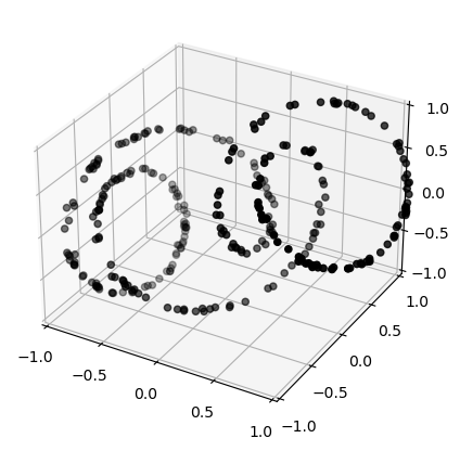
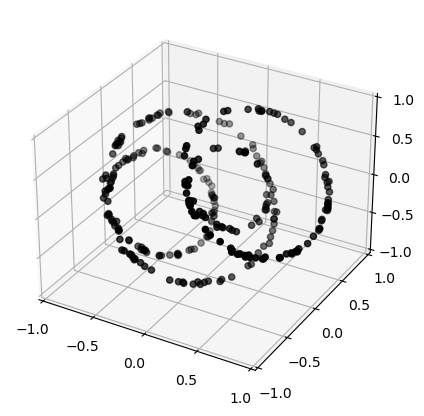
Figure 1: The input point cloud $X$, and its transformation after Step 1 (both projected in dimension $3$ through PCA for visualisation purposes).

3.3 Step 2: Lie-PCA

For Step 2, we consider the point cloud $X\subset\mathbb{R}^{n}$, having applied Step 1 or not, and wish to find $\mathfrak{sym}(\mathcal{O})$. We remind the reader that the symmetry group $\mathrm{Sym}(\mathcal{O})$ and its Lie algebra $\mathfrak{sym}(\mathcal{O})$ have been defined in Section 2.1.4. This step is based on the work developed in [15].

3.3.1  The Lie-PCA operator

Lie-PCA is based on the fact that, for all $x\in\mathcal{O}$, $\mathfrak{sym}(\mathcal{O})$ is contained in the set

$$S_{x}\mathcal{O}=\{A\in\mathrm{M}_{n}(\mathbb{R})\mid Ax\in\mathrm{T}_{x}\mathcal{O}\},$$

where $\mathrm{T}_{x}\mathcal{O}$ denotes the tangent space of the manifold $\mathcal{O}$ at $x$. As we have seen in Equation (2), $\mathfrak{sym}(\mathcal{O})$ is equal to the intersection $\cap_{x\in\mathcal{O}}S_{x}\mathcal{O}$. Now, having access only to the point cloud $X$, the authors of [15] propose to estimate $\mathfrak{sym}(\mathcal{O})$ via

$$\bigcap_{i=1}^{N}S_{x_{i}}\mathcal{O}=\ker\bigg{(}\sum_{i=1}^{N}\Pi\big{[}{(S_{x_{i}}\mathcal{O})^{\bot}}\big{]}\bigg{)},$$

where the projections $\Pi\big{[}(S_{x_{i}}\mathcal{O})^{\bot}\big{]}$ are seen as operators on $\mathrm{M}_{n}(\mathbb{R})$. In practice, the $S_{x_{i}}\mathcal{O}$ are unknown, and a robust estimation is to be found. It is shown that $\Pi_{(S_{x_{i}}\mathcal{O})^{\bot}}$ is equal to

$$A\mapsto\Pi\big{[}\mathrm{N}_{x_{i}}\mathcal{O}\big{]}\cdot A\cdot\Pi\big{[}\langle x_{i}\rangle\big{]},$$

where $\mathrm{N}_{x_{i}}\mathcal{O}$ is the normal space of $\mathcal{O}$ at $x_{i}$, $\langle x_{i}\rangle$ is the line spanned by $x_{i}$, and $\Pi\big{[}\mathrm{N}_{x_{i}}\mathcal{O}\big{]}$ and $\Pi\big{[}\langle x_{i}\rangle\big{]}$ denotes the projection matrices on these subspaces. By denoting $\widehat{\Pi}\big{[}\mathrm{N}_{x_{i}}X\big{]}$ an estimation of $\Pi_{\mathrm{N}_{x_{i}}\mathcal{O}}$ computed from the observation $X$, we replace the previous operator with

$$A\mapsto\widehat{\Pi}\big{[}\mathrm{N}_{x_{i}}X\big{]}\cdot A\cdot\Pi\big{[}\langle x_{i}\rangle\big{]}.$$

Further details on the estimation of normal spaces are provided below. Combining all the aforementioned aspects, a reliable estimation of $\mathfrak{sym}(\mathcal{O})$ can be obtained by computing the kernel of the operator $\Lambda\colon\mathrm{M}_{n}(\mathbb{R})\rightarrow\mathrm{M}_{n}(\mathbb{R})$ defined as

$$\Lambda(A)=\sum_{i=1}^{N}\widehat{\Pi}\big{[}\mathrm{N}_{x_{i}}X\big{]}\cdot A\cdot\Pi\big{[}\langle x_{i}\rangle\big{]}.$$

More accurately, $\mathfrak{sym}(\mathcal{O})$ should be sought as the linear subspace of $\mathrm{M}_{n}(\mathbb{R})$ spanned by the eigenvectors associated with almost-zero eigenvalues of $\Lambda$. We stress that $\Lambda$ is a symmetric operator, hence diagonalizable when seen as a $n^{2}\times n^{2}$ matrix.

3.3.2  Estimation of normal spaces

We now turn to the estimations $\widehat{\Pi}\big{[}\mathrm{N}_{x_{i}}X\big{]}$ of the normal spaces $\Pi\big{[}\mathrm{N}_{x_{i}}\mathcal{O}\big{]}$. First, we note that the problem of estimation of normal spaces is equivalent to the one for tangent spaces, since we have the relation

$$\Pi\big{[}\mathrm{T}_{x_{i}}\mathcal{O}\big{]}+\Pi\big{[}\mathrm{N}_{x_{i}}\mathcal{O}\big{]}=I$$

with $I$ the identity matrix. Indeed, $\mathrm{T}_{x_{i}}\mathcal{O}$ and $\mathrm{N}_{x_{i}}\mathcal{O}$ are complementary orthogonal subspaces. Now, estimating tangent spaces can be done through the common technique of local PCA [88, 52, 1, 60]. Given a real number $r>0$, called the scale parameter, this technique first computes the local covariance matrix of $X$ at scale $r$ and centered at $x_{i}$, defined as

$$\Sigma_{x_{i}}^{r}[X]=\frac{1}{|Y|}\sum_{y\in Y}(y-x_{i})(y-x_{i})^{\top},$$ (13)

where $Y=\{y\in X\mid\|y-x_{i}\|\leq r\}$ is the set of input points at distance at most $r$ from $x_{i}$. Now, given the dimension $l$ of $\mathcal{O}$, known in advance or estimated, we estimate $\mathrm{T}_{x_{i}}\mathcal{O}$ via the space spanned by the $l$ bottom eigenvectors of $\Sigma_{x_{i}}^{r}[X]$. In what follows, we denote by $\Pi_{x_{i}}^{l,r}[X]$ the projection on this space. We eventually consider the estimator

$$\widehat{\Pi}\big{[}\mathrm{N}_{x_{i}}X\big{]}=I-\Pi_{x_{i}}^{l,r}[X].$$

Due to the popularity of local PCA, probabilistic guarantees for this procedure can be found in several works, such as those cited above. Moreover, closely related variations have been studied, obtained by weighting the matrix $\Sigma_{x_{i}}^{r}[X]$, or by using $k$-neighbors [79, 15]. All of these works, however, state their results in probability, and not as deterministic inequalities, as we will need when analyzing our algorithm. This will be remedied in Section 5.2.3, which contains deterministic stability results for $\Pi_{x_{i}}^{r,l}[X]$ with respect to Wasserstein distance.

In actual implementations, the set $Y$ is obtained using the binary tree algorithm [10] from the Python library scikit-learn [71]. Besides, we stress that the accuracy of local PCA, in addition to its dependence on the geometry of $\mathcal{O}$ and the density of $X$, is highly affected by the parameter $r$, since too small values imply large variance, whereas bigger ones give biased estimations. We will derive in Lemmas 5.12 and 5.13 a theoretical range in which $r$ should be chosen, although, in practice, there is little ad hoc guidance in the choice.

3.3.3  Implementation

As presented in the original paper, the last step of Lie-PCA consists in computing the linear subspace of $\mathrm{M}_{n}(\mathbb{R})$ spanned by the $l$ bottom eigenvectors of $\Lambda$, offering an estimation of $\mathfrak{sym}(\mathcal{O})$. This procedure, however, is not suited to our context, since we seek $\mathfrak{h}$, which is only a subalgebra of $\mathfrak{sym}(\mathcal{O})$. An example is given by the unit sphere $S^{3}\subset\mathbb{R}^{4}$, which is an orbit of a representation of $\mathrm{SU}(2)$, but whose symmetry group is $\mathrm{SO}(4)$, of higher dimension. In this case, the inclusion of $\mathfrak{h}=\mathfrak{su}(2)$ in $\mathfrak{sym}(S^{3})=\mathfrak{so}(4)$ is not an equality. Consequently, instead of computing the eigenvectors of $\Lambda$, we simply compute the values it takes on the canonical basis of $\mathrm{M}_{n}(\mathbb{R})$, and save them in a $n^{2}\times n^{2}$ matrix. This will allow us, in Step 3, to propose an estimation for $\mathfrak{h}$. Our implementation of Lie-PCA is given in Algorithm 3.3.3 below. In addition, we illustrate some applications of Lie-PCA in Example 3.3.

   2 Step 2 of Algorithm 3.1 (Lie-PCA)

 

1:A point cloud $X=\{x_{i}\}_{i=1}^{N}$ in $\mathbb{R}^{n}$, a real number $r>0$ and an integer $l$.

2:The Lie-PCA operator $\Lambda$ computed in the canonical basis of $\mathrm{M}_{n}(\mathbb{R})$.

3:for $i=1,\dots,N$ do

4:     let $\overline{\Sigma}_{x_{i}}^{r}[X]$ be the local covariance matrix at scale $r$, as in Equation (13)

5:     let $\Pi_{x_{i}}^{l,r}[X]$ be the projection on its $l$ bottom eigenvectors

6:     $\widehat{\Pi}\big{[}\mathrm{N}_{x_{i}}X\big{]}\leftarrow I-\Pi_{x_{i}}^{l,r}[X]$

7:end for

8:$\Lambda\leftarrow\bigg{[}\sum_{i=1}^{N}\widehat{\Pi}\big{[}\mathrm{N}_{x_{i}}X\big{]}\cdot A_{v,w}\cdot\Pi\big{[}\langle x_{i}\rangle\big{]}\bigg{]}_{1\leq i,j\leq n}$ for $A_{v,w}$ the $(v,w)$-th canonical vector of $\mathrm{M}_{n}(\mathbb{R})$

 

Example 3.3.

Figure 2 illustrates applications of Lie-PCA to point clouds sampled on a circle in $\mathbb{R}^{2}$, a flat torus in $\mathbb{R}^{4}$, and a sphere in $\mathbb{R}^{3}$. They consist respectively of $100$, $500$ and $500$ points. These spaces correspond to orbits of representations of the Lie groups $\mathrm{SO}(2)$, $T^{2}$, and $\mathrm{SO}(3)$ respectively, which are also their symmetry groups. The algorithm shows excellent performance, as evidenced by the fact that the operator $\Lambda$ exhibits a few significantly small eigenvalues, the number of which corresponds to the dimension of the corresponding Lie group.

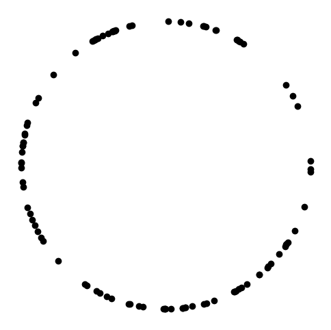
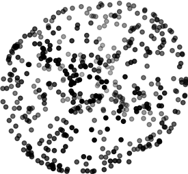
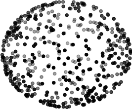
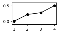
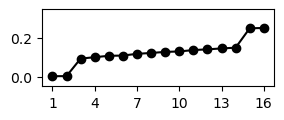
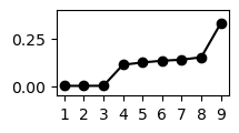
Figure 2: Results of Lie-PCA to data points sampled around the unit circle in $\mathbb{R}^{2}$ (left), the unit torus in $\mathbb{R}^{4}$ (middle, with data set reduced to dimension 3 through PCA for visualization purposes), and the unit sphere in $\mathbb{R}^{3}$ (right). One can infer the respective Lie algebra dimensions to be 1, 2, and 3 based on the graphs of eigenvalues of the matrix $\Lambda$, represented at the bottom.

Example 3.4.

We apply Step 2 to the point cloud $X$ presented in Example 3.1. The Lie-PCA operator has the following eigenvalues, given with 3 decimal places:

$$0.001,~{}0.102,~{}0.109,~{}0.112,~{}0.135,~{}0.145,~{}0.156,~{}0.212,$$

$$0.212,~{}0.233,~{}0.236,~{}0.247,~{}0.249,~{}0.259,~{}0.296,~{}0.296.$$

One is significantly small, suggesting that the symmetry group has dimension $1$, as expected.

3.4 Step 3: Closest Lie algebra

For the third step, we seek a Lie subalgebra $\widehat{\mathfrak{h}}$ of $\mathfrak{sym}(\mathcal{O})$ isomorphic to $\mathfrak{h}$. We propose two variations of this step: a general algorithm, and another one, valid only when $\mathfrak{h}=\mathfrak{sym}(\mathcal{O})$.

3.4.1  Formulation of the problem

As mentioned previously, $\mathfrak{sym}(\mathcal{O})$ can be estimated as the kernel of the Lie-PCA operator $\Lambda\colon\mathrm{M}_{n}(\mathbb{R})\rightarrow\mathrm{M}_{n}(\mathbb{R})$, or more exactly, as the set of matrices $A\in\mathrm{M}_{n}(\mathbb{R})$ for which $\|\Lambda(A)\|/\|A\|$ is small. However, Lie-PCA does not involve any information regarding the commutators, i.e., it only allows to estimate $\mathfrak{sym}(\mathcal{O})$ as if it were a linear subspace. In order to find $\mathfrak{h}$, one has to force a Lie algebra structure. This is done through $\mathcal{V}(G,\mathfrak{so}(n))$, the Stiefel variety of Lie subalgebras of $\mathfrak{so}(n)$ that are pushforwards by almost-faithful representations of $G$ (see Section 2.3.2). Its elements are the $d$-frames $(A_{1},\dots,A_{d})$ of $\mathfrak{so}(n)$ spanning a subalgebra isomorphic to $\mathfrak{g}$. We are invited to consider the program

$$\arg\min\sum_{i=1}^{d}\|\Lambda(A_{i})\|^{2}\;\;\;\text{s.t. }(A_{1},\dots,A_{d})\in\mathcal{V}(G,\mathfrak{so}(n)).$$ (14)

In order to implement this problem, the structure of $\mathcal{V}(G,\mathfrak{so}(n))$ must be known. This analysis has already been given in Section 2.3, and we summarize it now. The set $\mathfrak{orb}(G,n)$, defined in Equation (6), consists of a choice of tuples $\big{(}B^{\phi_{1}},\dots,B^{\phi_{p}}\big{)}$, where $(\phi_{1},\dots,\phi_{p})$ is a collection of irreducible representations of $G$ such that their sum $\bigoplus_{k=1}^{p}\phi_{k}$ has dimension $n$ and is orthogonal and almost-faithful, and where $B^{\phi}$ is defined as

$$B^{\phi}=\big{(}\mathrm{d}\phi(e_{1}),\dots,\mathrm{d}\phi(e_{d})\big{)},$$

for a fixed basis $(e_{i})_{i=1}^{d}$ of $\mathfrak{g}$. Moreover, the elements of $\mathfrak{orb}(G,n)$ have been chosen so as to generate non-orbit-equivalent representations (defined in Section (2.2.3)). Based on this initial set of tuples of irreducible representations, we have seen a few operations to generate new Lie algebras: their direct sum, the right-multiplication by a matrix $P\in\mathrm{O}(d)$, and the conjugation by a matrix $O\in\mathrm{O}(n)$. Moreover, as stated in Lemma 2.10, any element $(A_{1},\dots,A_{d})$ of $\mathcal{V}(G,\mathfrak{so}(n))$ can be obtained via this process: there exists a collection $(B^{1},\dots,B^{p})\in\mathfrak{orb}(G,n)$, and two matrices $P\in\mathrm{O}(d)$ and $O\in\mathrm{O}(n)$ such that, for all $i\in[1\dots d]$, we have

$$A_{i}=\sum_{j=1}^{d}P_{j,i}C_{j}~{}~{}~{}~{}~{}\mathrm{where}~{}~{}~{}~{}~{}C_{j}=O\mathrm{diag}\big{(}B^{k}_{j}\big{)}_{k=1}^{p}O^{\top}.$$

By injecting this expression in Equation (14), we observe a simplification:

$$\sum_{i=1}^{d}\bigg{\|}\Lambda\bigg{(}\sum_{j=1}^{d}P_{j,i}C_{j}\bigg{)}\bigg{\|}^{2} =\sum_{i=1}^{d}\sum_{j=1}^{d}\bigg{(}P_{j,i}^{2}\big{\|}\Lambda\big{(}C_{j}\big{)}\big{\|}^{2}+\sum_{j^{\prime}\neq j}P_{j,i}P_{j^{\prime},i}\big{\langle}\Lambda\big{(}C_{j}\big{)},\Lambda\big{(}C_{j^{\prime}}\big{)}\big{\rangle}\bigg{)}$$

$$=\sum_{j=1}^{d}\sum_{i=1}^{d}P_{j,i}^{2}\big{\|}\Lambda\big{(}C_{j}\big{)}\big{\|}^{2}+\sum_{j=1}^{d}\sum_{j^{\prime}\neq j}\sum_{i=1}^{d}P_{j,i}P_{j^{\prime},i}\big{\langle}\Lambda\big{(}C_{j}\big{)},\Lambda\big{(}C_{j^{\prime}}\big{)}\big{\rangle}$$

$$=\sum_{j=1}^{d}\big{\|}\Lambda\big{(}C_{j}\big{)}\big{\|}^{2}+0,$$

where we used on the last line the orthonormality of the rows of $P$. We deduce that the minimization problem is independent of the matrix $P$ chosen. Thus, we have the equivalent formulation of Equation (14), already stated in Equation (9):

$$\arg\min\sum_{j=1}^{d}\bigg{\|}\Lambda\bigg{(}O\mathrm{diag}\big{(}B^{k}_{j}\big{)}_{k=1}^{p}O^{\top}\bigg{)}\bigg{\|}^{2}\;\;\;\text{s.t. }\begin{cases}(B^{1},\dots,B^{p})\in\mathfrak{orb}(G,n),\\ O\in\mathrm{O}(n).\end{cases}$$

By definition of $\mathfrak{orb}(G,n)$, the tuples $(B^{1},\dots,B^{p})$ come from irreducible representations $(\phi_{1},\dots,\phi_{p})$, such that such that the corresponding Lie algebra is a $d$-dimensional subset of $\mathfrak{so}(n)$. Moreover, only one representative for each orbit-equivalence class is chosen. Let us denote by $|\mathfrak{orb}(G,n)|$ its cardinal. The program above naturally splits into $|\mathfrak{orb}(G,n)|$ minimization problems on $\mathrm{O}(n)$. In practice, such minimizations can be performed by gradient descent, as described in [2]. For the actual implementation, we used the Python package Pymanopt [87], which uses as a retraction map the so-called QR retraction [2]. Since the manifold $\mathrm{O}(n)$ is not connected, we minimization must be run twice: on $\mathrm{SO}(n)$ and on its complement. We then save the smallest cost. Algorithm 3.4.1 summarizes the steps necessary for solving this problem.

It is worth noting that a specific problem comes up when the Lie group $G$ is Abelian: the set of non-orbit-equivalent representations of $G$ in $\mathbb{R}^{n}$ may be infinite, as soon as $n\geq 4$. To circumvent this issue, we simply consider a finite number of them. In practice, we fix an integer $\omega_{\mathrm{max}}$, considered as a hyperparameter, and work with the irreducible representations whose weights are lower than $\omega_{\mathrm{max}}$ in absolute value. In Section 4, we will describe explicitly the set $\mathfrak{orb}(G,n)$ in the case of $\mathrm{SO}(2)$, $T^{d}$, $\mathrm{SU}(2)$ and $\mathrm{SO}(3)$, allowing to put the algorithm in practice.

   3 Pushforward Lie algebra of $G$ minimizing $\Lambda$ (Step 3 of Algorithm 3.1)

 

1:The Lie-PCA operator $\Lambda$ computed in the canonical basis of $\mathrm{M}_{n}(\mathbb{R})$, a compact Lie group $G$ of dimension $d$, and a list $\mathfrak{orb}(G,n)$ of pushforward algebras of tuples of irreps.

2:A basis $A^{*}=(A_{1}^{*},\dots,A_{d}^{*})$ formed by direct sum, right-multiplication, and conjugation of elements in $\mathfrak{orb}(G,n)$, that minimizes Equation (9).

3:Let L be the list of tuples $(A_{1}^{\phi},\dots,A_{d}^{\phi})$ obtained from the $(B^{\phi_{1}},\dots,B^{\phi_{p}})$’s in $\mathfrak{orb}(G,n)$ by putting $A_{j}^{\phi}=\mathrm{diag}\big{(}B^{\phi_{1}}_{j},\dots,B^{\phi_{p}}_{j}\big{)}$, and where $\phi=\bigoplus_{k=1}^{p}\phi_{k}$.

4:for $(A_{1}^{\phi},\dots,A_{d}^{\phi})$ in L do

5:     solve $~{}~{}~{}\mathrm{cost(\phi)}\leftarrow\arg\min\sum_{j=1}^{d}\big{\|}\Lambda\big{(}OA_{j}^{\phi}O^{\top}\big{)}\big{\|}^{2}~{}~{}~{}$ constrained to $O\in\mathrm{O}(n)$. Denote the minimizer as $O_{\phi}$.

6:end for

7:$\phi^{*}\leftarrow$ minimizer of cost.

8:$A^{*}\leftarrow(O_{\phi^{*}}A^{\phi^{*}}_{1}O_{\phi^{*}}^{\top},\dots,O_{\phi^{*}}A^{\phi^{*}}_{d}O_{\phi^{*}}^{\top})$.

 

Example 3.5.

Still considering the point cloud $X$ presented in Example 3.1, we apply Step 3 with $G=\mathrm{SO}(2)$, and with weights at most $\omega_{\mathrm{max}}=4$. There are 6 classes of orbit-equivalent representations of $\mathrm{SO}(2)$ in $\mathbb{R}^{4}$ with such weights. For each of them, we compute the minimum of Equation (9), and write it in the following table. We check that the algorithm correctly points the representation $\phi_{1}\oplus\phi_{4}$ as the most likely to generate the orbit underlying the points.

Weights	$(0,1)$	$(1,2)$	$(1,3)$	$(1,4)$	$(2,3)$	$(3,4)$
Costs	$0.003$	$0.002$	$0.0003$	$6.635\times 10^{-6}$	$0.006$	$0.009$

3.4.2  Other formulation of the problem

As mentioned earlier, in the original paper of Lie-PCA, the authors propose to estimate $\mathfrak{sym}(\mathcal{O})$ as $\langle A_{1},\dots,A_{d}\rangle$, the linear subspace of $\mathrm{M}_{n}(\mathbb{R})$ spanned by the $d$ bottom eigenvectors of $\Lambda$, where $d$ is a parameter, supposedly equal to the dimension of $\mathfrak{sym}(\mathcal{O})$. In certain cases, such as those of Example 3.3, $\mathfrak{sym}(\mathcal{O})$ has the dimension of $G$, hence $\langle A_{1},\dots,A_{d}\rangle$ can serve as an estimator of $\mathfrak{h}$. In this paragraph, we will suppose that it is the case. As raised by the authors, this linear subspace may not form a Lie algebra, in the sense that it may not be close under Lie bracket. Hence a natural step would consist in projecting $\langle A_{1},\dots,A_{d}\rangle$ onto the ‘closest Lie algebra’, which is left as an open question. As it turns out, a variation of Algorithm 3.4.1 gives a partial answer to this problem. Namely, by denoting $\mathcal{G}^{\text{Lie}}(d,\mathfrak{so}(n))$ the set of $d$-dimensional Lie subalgebras of $\mathfrak{so}(n)$ (introduced in Section 2.3.1), we are compelled to solve the program

$$\arg\min\big{\|}\Pi\big{[}\langle A_{i}\rangle_{i=1}^{d}\big{]}-\Pi\big{[}\mathfrak{h}\big{]}\big{\|}~{}~{}~{}~{}\text{s.t. }~{}~{}~{}~{}\mathfrak{h}\in\mathcal{G}^{\text{Lie}}(d,\mathfrak{so}(n)),$$

where we recall that, as it is common in the literature, we compute the distance between spaces as the Frobenius distance between their projection matrices. Here, we consider subspaces of $\mathfrak{so}(n)$, hence the corresponding projection matrices have size $n(n-1)/2\times n(n-1)/2$.

Unfortunately, due to the intricate nature of the space $\mathcal{G}^{\text{Lie}}(d,\mathfrak{so}(n))$, we were not able to find a way to directly minimize this problem. To circumvent this issue, we restrict $\mathcal{G}^{\text{Lie}}(d,\mathfrak{so}(n))$ to $\mathcal{G}(G,\mathfrak{so}(n))$, the set of Lie subalgebras of $\mathfrak{so}(n)$ coming from an almost-faithful representation of $G$ in $\mathbb{R}^{n}$, defined in Section 2.3.2. We are invited to consider the second problem

$$\arg\min\big{\|}\Pi\big{[}\langle A_{i}\rangle_{i=1}^{d}\big{]}-\Pi\big{[}\mathfrak{h}\big{]}\big{\|}~{}~{}~{}~{}\text{s.t. }~{}~{}~{}~{}\mathfrak{h}\in\mathcal{G}(G,\mathfrak{so}(n)).$$

which, this time, can be solved. Indeed, as a consequence of Lemma 2.10, any element of $\mathfrak{h}\in\mathcal{G}(G,\mathfrak{so}(n))$ can be obtained via a process similar to what has been described previously. Explicitly, there exists a $p$-tuple $(B^{1},\dots,B^{p})\in\mathfrak{orb}(G,n)$ and a matrix $O\in\mathrm{O}(n)$ such that the $d$-tuple $(O\mathrm{diag}(B^{\phi_{k}}_{1})_{k=1}^{p}O^{\top},\dots,O\mathrm{diag}(B^{\phi_{k}}_{d})_{k=1}^{p}O^{\top})$ forms a basis of $\mathfrak{h}$. Consequently, the minimization problem above can be decomposed into Equation (10) already mentioned:

$$\arg\min\big{\|}\Pi\big{[}\langle A_{i}\rangle_{i=1}^{d}\big{]}-\Pi\big{[}\langle O\mathrm{diag}(B^{k}_{i})_{k=1}^{p}O^{\top}\rangle_{i=1}^{d}\big{]}\big{\|}\;\;\;\text{s.t. }\begin{cases}(B^{1},\dots,B^{p})\in\mathfrak{orb}(G,n),\\ O\in\mathrm{O}(n).\end{cases}$$

This program naturally splits into $|\mathfrak{orb}(G,n)|$ minimization problems over $\mathrm{O}(n)$, just as it was the case for the minimization of Step 3, given in Equation (9).

We see that formulated as it is, the computational complexity of Step 3 and Step 3’ are comparable. In practice, we observed that performing a minimization over $\mathrm{O}(n)$ for the latter problem is slightly faster, this being due to the fact that the term in Equation (10) is less costly to calculate than in (9). Being slightly faster is, however, not the main interest of Step 3’. As we will develop in Sections 4.1.2 and 4.2.2, Equation (10) admits a convenient formulation in the case where $G$ is the torus, enabling us to derive a more reliable and significantly faster algorithm. We stress, nonetheless, that it comes at the cost of a theoretical limitation: when the Lie algebra $\mathfrak{h}$ is a strict subset of $\mathfrak{sym}(\mathcal{O})$, that is, when $d<\dim(\mathfrak{sym}(\mathcal{O}))$, then the $d$ bottom eigenvectors of $\Lambda$ may not cover $\mathfrak{h}$, hence the minimizer of Equation (10) may not be close.

We provide a high-level implementation of this program in Algorithm 3.4.2. As a technical detail, we point out that the bottom eigenvectors of the Lie-PCA operator may not be skew-symmetric matrices. This is corrected by the first two lines of the algorithm. In practice, as for all optimization problems of this paper, we use gradient descent, implemented in the Python package Pymanopt [87].

   4 Projection on closest pushforward Lie algebra of $G$ (Step 3’ of Algorithm 3.1)

 

1:An orthonormal basis $\{A_{i}\}_{i=1}^{d}$ for the estimated pushforward algebra in Step 2, a compact Lie group $G$ of dimension $d$, and a list $\mathfrak{orb}(G,n)$ of pushforward algebras of tuples of irreps.

2:A basis $A^{*}=(A_{1}^{*},\dots,A_{d}^{*})$ formed by direct sum, right-multiplication, and conjugation of elements in $\mathfrak{orb}(G,n)$, that minimizes Equation (10).

3:Make the basis $\{A_{i}\}_{i=1}^{d}$ skew-symmetric via $A_{i}\leftarrow\frac{1}{2}(A_{i}-A_{i}^{T})$

4:$\{A_{i}\}_{i=1}^{d}\leftarrow\text{Gram-Schmidt process applied to }\{A_{i}\}_{i=1}^{d}$;

5:Let L be the list of tuples $(A_{1}^{\phi},\dots,A_{d}^{\phi})$ obtained from the $(B^{\phi_{1}},\dots,B^{\phi_{p}})$’s in $\mathfrak{orb}(G,n)$ by putting $A_{j}^{\phi}=\mathrm{diag}\big{(}B^{\phi_{1}}_{j},\dots,B^{\phi_{p}}_{j}\big{)}$, and where $\phi=\bigoplus_{k=1}^{p}\phi_{k}$.

6:for $(A_{1}^{\phi},\dots,A_{d}^{\phi})$ in L do

7:     solve $~{}~{}~{}\mathrm{cost(\phi)}\leftarrow\arg\min\big{\|}\Pi\big{[}\langle A_{i}\rangle_{i=1}^{d}\big{]}-\Pi\big{[}\langle OA_{i}^{\phi}O^{\top}\rangle_{i=1}^{d}\big{]}\big{\|}~{}~{}~{}$ constrained to $O\in\mathrm{O}(n)$. Denote the minimizer as $O_{\phi}$.

8:end for

9:$\phi^{*}\leftarrow$ minimizer of cost.

10:$A^{*}\leftarrow(O_{\phi^{*}}A^{\phi^{*}}_{1}O_{\phi^{*}}^{\top},\dots,O_{\phi^{*}}A^{\phi^{*}}_{d}O_{\phi^{*}}^{\top})$.

 

Example 3.6.

We reproduce the same experiment as Example 3.5, now with Step 3’ instead of Step 3. For each of the $6$ non-orbit-equivalent representations of $\mathrm{SO}(2)$ in $\mathbb{R}^{4}$ with weights at most $4$, we compute the minimum of Equation (10), and write it in the following table. As expected, the representation $\phi_{1}\oplus\phi_{4}$ yields the minimal cost.

Weights	$(0,1)$	$(1,2)$	$(1,3)$	$(1,4)$	$(2,3)$	$(3,4)$
Costs	$0.004$	$0.002$	$0.002$	$4.29\times 10^{-5}$	$0.006$	$0.008$

3.5 Step 4: Distance to orbit

In the previous step, we have calculated the representation $\widehat{\phi}\colon G\rightarrow\mathrm{SO}(n)$ whose pushforward Lie algebra $\widehat{\mathfrak{h}}$ is closest to creating an orbit underlying the point cloud $X$, with closeness being computed at the level of Lie algebras. We now end our algorithm with a verification step, namely, we check whether $\widehat{\phi}$ does indeed generate an orbit containing $X$. To this end, we propose two alternatives: using the Hausdorff distance or the Wasserstein distance, both popular measures of distance in the literature. The orbit is defined as

$$\widehat{\mathcal{O}}_{x}=\widehat{\phi}(G)\cdot x=\big{\{}\exp(A)x\mid A\in\widehat{h}\big{\}},$$

where $\exp$ denotes the matrix exponential, and where $x$ is taken as any point of $X$.

3.5.1  Hausdorff distance

It is a measure of proximity between the subsets of the Euclidean space. Since the point cloud $X$ is thought as only a subset of the orbit, it is more appropriate to consider the non-symmetric Hausdorff distance $\mathrm{d}_{\mathrm{H}}\big{(}X|\widehat{\mathcal{O}}_{x}\big{)}$, defined as

$$\mathrm{d}_{\mathrm{H}}\big{(}A|B\big{)}=\adjustlimits{\sup}_{a\in A}{\inf}_{b\in B}\|a-b\|.$$

Note that we recover the (usual) Hausdorff distance as

$$\mathrm{d}_{\mathrm{H}}\big{(}A,B\big{)}=\max\{\mathrm{d}_{\mathrm{H}}\big{(}A|B\big{)},\mathrm{d}_{\mathrm{H}}\big{(}B|A\big{)}\}.$$

In practice, the distance between the subsets $\widehat{\mathcal{O}}_{x}$ and $X=\{x_{i}\}_{i=1}^{N}$ cannot be calculated directly, since $\widehat{\mathcal{O}}_{x}$ is a continuous manifold. This can be remedied through an approximation, by sampling a large but finite set of points on $\widehat{\mathcal{O}}_{x}$ and computing the distance between the finite sets. In this regard, efficient methods for computing the distance are described in [82], and implemented in the package SciPy in Python, that we use.

To generate a finite sample of $\widehat{\mathcal{O}}_{x}$, we use the surjectivity of the exponential map $\exp\colon\mathfrak{g}\rightarrow G$. As presented in Section 2.1.1. we have a commutative diagram

Moreover, let $\mathrm{diam}(G)$ denote the diameter of $G$, when endowed with a bi-invariant Riemannian structure, as discussed in Section 2.1.3. By definition of the diameter, the image of a ball of radius $\mathrm{diam}(G)$ around the origin of $\mathfrak{g}$ covers the whole group $G$. If $\delta$ is a Lispchitz constant for $\widehat{\phi}$, we deduce that matrix exponential of a ball of radius $\delta\times\mathrm{diam}(G)$ around the origin of $\mathfrak{h}$ will also cover the whole image $\phi(G)$, In other words, we have a parametrization

$$\widehat{\mathcal{O}}_{x}=\big{\{}\exp(A)x\mid A\in\mathfrak{h},\|A\|\leq\delta\times\mathrm{diam}(G)\big{\}}.$$

The Lie algebra $\mathfrak{h}$ being a $d$-dimensional vector subspace of $\mathfrak{so}(n)$, we can easily sample points on it, and deduce a sample of $\widehat{\mathcal{O}}_{x}$. More precisely, we consider a basis $\{A_{i}\}_{i=1}^{d}$ of $\mathfrak{h}$, choose a large and regularly-spaced finite subset of the unit sphere $S^{d}$ of $\mathbb{R}^{d}$, and build

$$\bigg{\{}\exp\bigg{(}\delta\times\mathrm{diam}(G)\sum_{i=1}^{d}t_{i}A_{i}\bigg{)}\cdot x\mid(t_{1}\dots,t_{d})\in S^{d}\bigg{\}}\subset\widehat{\mathcal{O}}_{x}.$$ (15)

We illustrate this procedure in Example 3.7.

Let us now suppose that the Hausdorff distance $\mathrm{d}_{\mathrm{H}}\big{(}X|\widehat{\mathcal{O}}_{x}\big{)}$ has been computed. Because a ‘close enough’ distance grows with dimension, it is not trivial to establish fixed thresholds to separate what are data close enough to an orbit to be considered a sample from it or not. In practice, one may vary the number of samples used in the estimation of the orbit, and observe whether or not the distance converges to a small error value. As another answer to this problem, we could compare $\mathrm{d}_{\mathrm{H}}\big{(}X|\widehat{\mathcal{O}}_{x}\big{)}$ to the theoretical upper bound given in Theorem 5.21. This bound, however, depends on certain unknown quantities, that would have to be estimated.

3.5.2  Wasserstein distance

Comparing the input data $X$ and the output orbit $\widehat{\mathcal{O}}_{x}$ can be realized, as an alternative, using the popular notion of distance offered by optimal transport. We recall that, given two probability measures $\mu$ and $\nu$ over $\mathbb{R}^{n}$, a transport plan between $\mu$ and $\nu$ is a probability measure $\pi$ over $\mathbb{R}^{n}\times\mathbb{R}^{n}$ whose marginals are $\mu$ and $\nu$. For any real number $p\geq 1$, the $p$-Wasserstein distance between $\mu$ and $\nu$ is defined as

$$\mathrm{W}_{p}(\mu,\nu)=\left(\inf_{\pi}\int\|x-y\|^{p}\mathrm{d}\pi(x,y)\right)^{\frac{1}{p}},$$

where the infimum is taken over all the transport plans $\pi$. An optimal transport plan is a $\pi$ that attains this infimum. If $q$ is such that $p\leq q$, then $\mathrm{W}_{p}(\mu,\nu)\leq\mathrm{W}_{q}(\mu,\nu)$ by Jensen’s inequality. In this article, we choose to work with the parameter $p=2$, which turned out to be the most convenient for deriving theoretical results in Section 5.

In this framework, we must associate probability measures to the subsets $X$ and $\widehat{\mathcal{O}}_{x}$. We choose for the former the empirical measure, defined as $\mu_{X}=\frac{1}{N}\sum_{i=1}^{N}\delta_{x_{i}}$, where $\delta$ denotes the Dirac mass. Regarding the latter, which is an orbit of $G$, a natural choice is the uniform measure $\mu_{\widehat{\mathcal{O}}_{x}}$. As defined in Section 2.2.3, it is the pushforward of the Haar measure on $G$:

$$\mu_{\widehat{\mathcal{O}}_{x}}=\big{(}\widehat{\phi}\cdot x\big{)}\mu_{G}.$$

In this context, the Wasserstein distance $\mathrm{W}_{2}\big{(}\mu_{X},\mu_{\widehat{\mathcal{O}}_{x}}\big{)}$ is a relevant measure of proximity, computing how close the supports $X$ and $\widehat{\mathcal{O}}_{x}$ are, and how uniform the distribution of $X$ is.

However, in the context of data analysis with the Wasserstein distance, it is common to allow $X$ to have a few anomalous points, that is, points far away from the underlying orbit $\mathcal{O}$. If $x$ is such a point, the estimated orbit $\widehat{\mathcal{O}}_{x}$ would not be a reliable approximation of $\mathcal{O}$. In order to circumvent this issue, we consider all the points of $X$, and define the average measure

$$\mu_{\widehat{\mathcal{O}}}=\frac{1}{N}\sum_{i=1}^{N}\mu_{\widehat{\mathcal{O}}_{x_{i}}}.$$

Eventually, the last step of our algorithm consists in computing $\mathrm{W}_{2}\big{(}\mu_{X},\mu_{\widehat{\mathcal{O}}}\big{)}$.

In practice, we face a problem similar to that of the Hausdorff distance: the support of $\mu_{\widehat{\mathcal{O}}}$ is infinite, and we are not aware of algorithms that would compute it exactly. Instead, we propose to use the approximation of Equation (15), so as to compute a finite sample on each orbit $\widehat{\mathcal{O}}_{x}$. We then gather all the samples in a set $\widehat{\mathcal{O}}^{\prime}$, and consider its empirical measure $\mu_{\widehat{\mathcal{O}}^{\prime}}$. The Wasserstein distance $\mathrm{W}_{2}\big{(}\mu_{X},\mu_{\widehat{\mathcal{O}}^{\prime}}\big{)}$, only involving discrete measures, can be computed using the package POT in Python [34], based on efficient implementations of the Sinkhorn algorithm, such as [24]. This is shown in Examples 3.7 and 3.8.

We stress that, compared to the Hausdorff distance, the Wasserstein distance has the advantage of being robust to the presence of outliers in $X$. Indeed, from its definition, we see that adding a few anomalous points to $X$ cannot change too much the value of $\mathrm{W}_{2}\big{(}\mu_{X},\mu_{\mathcal{O}}\big{)}$, hence the robustness against outliers. In Theorem 5.21, we will show that $\mathrm{W}_{2}\big{(}\mu_{X},\mu_{\widehat{\mathcal{O}}}\big{)}$ is small as long as the initial distance $\mathrm{W}_{2}\big{(}\mu_{X},\mu_{\mathcal{O}}\big{)}$ is, proving the robustness of our algorithm against anomalous points. This property is illustrated in Example 3.8, where we apply successfully the algorithm on a a data corrupted with noise. On the downside, we draw the reader’s attention to the fact that, in this framework, the point cloud $X$ is seen as a sample of the uniform distribution on $\mathcal{O}$, or a close distribution. It does not include the more general assumption of non-uniform distribution. In contrast, the Hausdorff distance is only sensible to the support, and may be small even when non-uniformly distributed.

Example 3.7.

We apply Step 4 on $X$, based on the optimal Lie algebra returned by Step 3 in Example 3.5. We select an arbitrary $x\in X$, and approximate the Hausdorff distance of Equation (11) by sampling $500$ points on the estimated orbit $\widehat{\mathcal{O}}_{x}$, yielding $\mathrm{d}_{\mathrm{H}}\big{(}X|\widehat{\mathcal{O}}_{x}\big{)}\approx 0.018$. As observed in Figure 3, $\widehat{\mathcal{O}}_{x}$ appears to fit $X$ correctly. Besides, to approximate the Wasserstein distance of Equation (12), we sample $50$ points on $\widehat{\mathcal{O}}_{x}$ for each $x\in X$, and obtain $\mathrm{W}_{2}\big{(}\mu_{X},\mu_{\widehat{\mathcal{O}}}\big{)}\approx 0.335$. In order to visualize the measure $\mu_{\widehat{\mathcal{O}}}$, we consider its kernel density estimator $f\colon\mathbb{R}^{4}\rightarrow[0,+\infty)$ with Gaussian kernel of bandwidth $0.1$, and represent its sublevel set $f^{-1}([0.5,+\infty))$. We observe on the figure its adequacy with $X$.

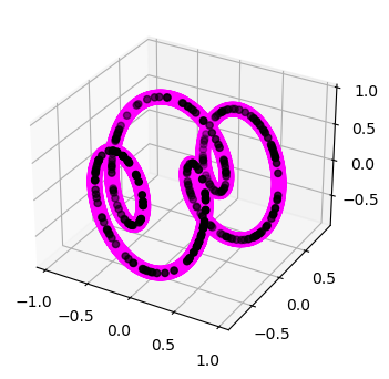
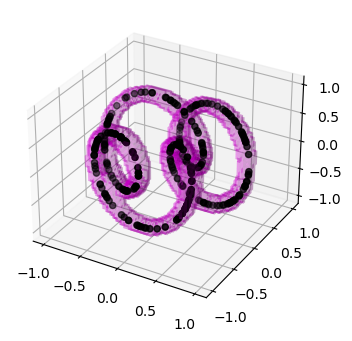
Figure 3: The point cloud $X$ in black, together with the estimated orbit $\widehat{\mathcal{O}}_{x}$ in magenta (left), and a sublevel set of a kernel density estimator on $\mu_{\widehat{\mathcal{O}}}$ (right).

Example 3.8.

We reproduce the running example of this section, starting from the same point cloud $X$ of cardinal $300$, presented in Example 3.1, to which we add an additive Gaussian noise of standard deviation $\sigma=0.03$, as well as $30$ points drawn uniformly in the cube $[-1,1]^{4}$. Algorithm 3.1 retrieves successfully the representation $\phi_{1}\oplus\phi_{4}$. However, by selecting an arbitrary $x\in X$, we obtain the Hausdorff distance $\mathrm{d}_{\mathrm{H}}\big{(}X|\widehat{\mathcal{O}}_{x}\big{)}\approx 1.128$, which we consider as large. It can be seen in Figure 4 that $\widehat{\mathcal{O}}_{x}$ does not fit $X$ correctly. On the other hand, the Wasserstein distance is $\mathrm{W}_{2}\big{(}\mu_{X},\mu_{\widehat{\mathcal{O}}}\big{)}\approx 0.392$, significantly better. We represent a sublevel set of a kernel density estimation on $\mu_{\widehat{\mathcal{O}}}$, similar to that of Example 3.7, which appears to match with $X$.

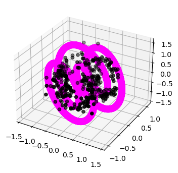
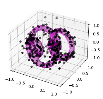
Figure 4: The corrupted version of the point cloud $X$ in black, together with the estimated orbit $\widehat{\mathcal{O}}_{x}$ in magenta (left), and a sublevel set of a kernel density estimator on $\mu_{\widehat{\mathcal{O}}}$ (right).

4 Additional algorithmic considerations

Algorithm 3.1, presented in the previous section, has to be adapted to the particular Lie group $G$ considered. More precisely, in Step 3, a list of irreps of $G$ must be provided, through the set $\mathfrak{orb}(G,n)$. In this section, we provide these lists in the case of $\mathrm{SO}(2)$, $T^{d}$, $\mathrm{SU}(2)$, and $\mathrm{SO}(3)$. Given any other group of interest, similar computations must be performed. However, it must be emphasized that, even if irreducible representations of compact Lie groups are well understood, it may be complicated to find explicit descriptions of them in the literature.

4.1 The algorithm for $\mathrm{SO}(2)$

We will observe that the set $\mathfrak{orb}(\mathrm{SO}(2),n)$ is closely linked to that of primitive integrals vectors, allowing an explicit description. We then propose a simplification of Step 3’.

4.1.1  Orbit-equivalence for $\mathrm{SO}(2)$

Let us recall the classification of irreps of $\mathrm{SO}(2)$, already given in Example 2.5: except the trivial representation $\phi_{0}\colon\mathrm{SO}(2)\rightarrow\mathrm{GL}_{1}(\mathbb{R})$, they are all of dimension $2$, and form the family $\{\phi_{k}\mid k\in\mathbb{Z}\setminus\{0\}\}$. In other words, irreps of $\mathrm{SO}(2)$ are parametrized by $\mathbb{Z}$, this parameter being called the weight. Let $n\geq 0$ be an integer. As a consequence of the decomposition into irreps, to any representation $\phi\colon\mathrm{SO}(2)\rightarrow\mathrm{GL}_{n}(\mathbb{R})$ corresponds a unique multiset $\{\{n_{1},\dots,n_{p}\}\}$ of integers such that $\phi$ is equivalent to the direct sum $\bigoplus_{k=1}^{p}\phi_{n_{k}}$. In order to simplify the notations to come, we will suppose that the dimension $n$ of the ambient space is even. In particular, $\{\{n_{1},\dots,n_{p}\}\}$ must contain an even number of zero values. The odd case $n+1$ is similar to that of $n$, since representations of $\mathrm{SO}(2)$ in $\mathbb{R}^{n+1}$ are obtained from representations of $\mathrm{SO}(2)$ in $\mathbb{R}^{n}$, to which we add the trivial representation $\phi_{0}$. In what follows, it will be convenient to denote by $\Lambda(\phi)$ the $(n/2)$-tuple containing all the nonzero integers in $\{\{n_{1},\dots,n_{p}\}\}$, and one zero for each pair of zeros. Let us write $\Lambda(\phi)=(k_{1},\dots,k_{n/2})$, whose ordering is, for the moment, arbitrary. We now suppose that the representation is orthogonal. Thus there exists an orthogonal matrix $O\in\mathrm{SO}(n)$ such that the pushforward Lie algebra $\mathfrak{h}=\mathrm{d}\phi(\mathfrak{g})$ is generated by the unit-norm skew-symmetric matrix $OB(k_{1},\dots,k_{n/2})O^{\top}$, where

$$B(k_{1},\dots,k_{n/2})=\frac{\mathrm{diag}\big{(}L(k_{1}),\dots,L(k_{n/2})\big{)}}{\sqrt{2}\big{\|}(k_{1},\dots,k_{n/2})\big{\|}}~{}~{}~{}~{}~{}\mathrm{and}~{}~{}~{}~{}~{}L(k)=\begin{pmatrix}0&-k\\ k&0\end{pmatrix}.$$ (16)

When the representation is trivial, we define $B(0,\dots,0)$ as the zero matrix.

We remind the reader that, as defined in Section 2.2.3, two representations $\phi$ and $\phi^{\prime}$ are said orbit-equivalent if there exists a matrix $O\in\mathrm{O}(n)$ such that $\mathrm{d}\phi(\mathfrak{g})=O\mathrm{d}\phi^{\prime}(\mathfrak{g})O^{\top}$. In the particular case of $\mathrm{SO}(2)$, we have a convenient equivalent characterization, that can be deduced from the equation above and the fact that conjugated matrices share the same eigenvalues. First of all, given a representation $\phi$, we can suppose that its weights $\Lambda(\phi)=(k_{1},\dots,k_{n/2})$ are non-negative and ordered, since this operation would yield an equivalent representation, hence orbit-equivalent. Moreover, two representations $\phi$ and $\phi^{\prime}$ are orbit-equivalent when there exists an $\alpha\in\mathbb{N}\setminus\{0\}$ such that $\Lambda(\phi)$ can be obtained from $\Lambda(\phi^{\prime})$ by multiplying each element by $\alpha$, or dividing each element by $\alpha$. We deduce that $\mathfrak{orb}(\mathrm{SO}(2),n)$ is in correspondence with the set of non-negative and ordered primitive integral vectors, defined as

$$\mathbb{N}^{n/2}_{\mathrm{prim}}=\big{\{}(k_{1},\dots,k_{n/2})\in\mathbb{N}^{n/2}\mid k_{1}\leq\dots\leq k_{n/2},~{}\mathrm{gcd}(k_{1},\dots,k_{n/2})=1\big{\}},$$

where we take $\mathrm{gcd}$ to denote the greatest common divisor. We deduce that, explicitely,

$$\mathfrak{orb}(\mathrm{SO}(2),n)=\big{\{}B(k_{1},\dots,k_{n/2})\mid(k_{1},\dots,k_{n/2})\in\mathbb{N}^{n/2}_{\mathrm{prim}}\big{\}}.$$

As a remark, we point out that $\mathbb{N}^{n/2}_{\mathrm{prim}}$ has been extensively studied in the context of Linnik’s problem in analytic number theory [61, 29, 28]. It is known that, as $r\to+\infty$, the sets

$$\big{\{}x/\|x\|\mid x\in\mathbb{N}^{n/2}_{\mathrm{prim}},~{}\|x\|\leq r\big{\}}$$

are equidistributed on the intersection of the sphere $S^{n/2-1}$ and the positive quadrant $H=\{(x_{1},\dots,x_{n/2})\in\mathbb{R}^{n/2}\mid 0\leq x_{1}\leq\dots\leq x_{n/2}\}$. That is to say, the sequence of empirical measures on these sets converge in distribution to the Lebsegue measure on $S^{n/2-1}\cap H$. We stress that the restriction to $H$ comes from the fact that, in our context, only nonnegative ordered primitive vectors are considered. In other words, the primitive vectors, in addition to being dense on the sphere, tend to be uniformly distributed.

Although we will not it use directly in this paper, the equidistribution property of $\mathbb{N}^{n/2}_{\mathrm{prim}}$ guides our intuition when defining, for a parameter $\omega_{\mathrm{max}}\in\mathbb{N}$, the set of orbit-equivalence classes of representations of weights at most $\omega_{\mathrm{max}}$:

$$\mathfrak{orb}(\mathrm{SO}(2),n,\omega_{\mathrm{max}})=\big{\{}B(k_{1},\dots,k_{n/2})\mid(k_{1},\dots,k_{n/2})\in\mathbb{N}^{n/2}_{\mathrm{prim}},~{}\max\{|k_{i}|\}_{k=1}^{n/2}\leq r\big{\}}.$$ (17)

Indeed, when running our algorithm, and as pointed out in Section 3.4.1, the infinite set $\mathfrak{orb}(\mathrm{SO}(2),n)$ must be restricted to a finite subset. Choosing the restriction above will tend to be ‘uniformly distributed’ on $\mathfrak{orb}(\mathrm{SO}(2),n)$. It will be studied further in Section 5.3.1, in the context of rigidity of Lie subalgebras.

Based on this explicit description of $\mathfrak{orb}(\mathrm{SO}(2),n)$, Step 3 of Algorithm 3.1 can be performed. An entire execution of the algorithm has already been given in Examples 3.1, 3.2, 3.4, 3.5 and 3.7, and we provide below the Examples 4.2 and 4.3.

4.1.2  Reformulation of Step 3’

The fact that $\mathfrak{so}(2)$ is one-dimensional allows for a significant simplification of the algorithm. To see so, we suppose that the first two steps have been performed. Instead of going through Step 3, we consider the variation Step 3’, presented in Section 3.4.2. Namely, we let $A$ be a unit eigenvector of the Lie-PCA operator $\Lambda$ associated to the smallest eigenvalue, skew-symmetrize it if it is not, and consider Equation (10), which reads

$$\arg\min\big{\|}\Pi\big{[}\langle A\rangle\big{]}-\Pi\big{[}\langle OB(k_{1},\dots,k_{n/2})O^{\top}\rangle\big{]}\big{\|}^{2}\;\;\;\text{s.t. }\begin{cases}(k_{1},\dots,k_{n/2})\in\mathbb{N}^{n/2}_{\mathrm{prim}},\\ O\in\mathrm{O}(n).\end{cases}$$

According to Lemma 2.9, this distance on the Grassmannian can be reformulated as

$$2\big{\|}A\pm OB(k_{1},\dots,k_{n/2})O^{\top}\big{\|}^{2},$$ (18)

where the sign is chosen so as to minimize the norm. A tuple $(k_{1},\dots,k_{n/2})$ being fixed, we recognize in Equation (18) what is known in the literature as the two-sided orthogonal Procrustes problem with one transformation: given two matrices $A$ and $B$, find an orthogonal matrix $O$ that minimizes $\|A-OBO^{T}\|$. When both matrices $A$ and $B$ are symmetric, it has been shown that the problem admits an explicit solution, based on the best pairing between their eigenvalues [76, 89]. In our context, the matrices are skew-symmetric, but the problem can be solved in a similar fashion. First, we consider the normal form of $A$: there exists a matrix $P\in\mathrm{O}(n)$ and $n/2$ non-negative real numbers $\alpha_{1}\leq\dots\leq\alpha_{n/2}$ such that

$$A=PB(\alpha_{1},\dots,\alpha_{n/2})P^{\top}.$$

Consider a weight $(k_{1},\dots,k_{n/2})\in\mathbb{N}^{n/2}_{\mathrm{prim}}$. By Hoffman-Wielandt inequality [46], the quantity

$$\big{\|}PB(\alpha_{1},\dots,\alpha_{n/2})P^{\top}-OB(k_{1},\dots,k_{n/2})O^{\top}\big{\|}^{2}$$

is lower bounded by $2\big{\|}x/\|x\|-y/\|y\|\big{\|}^{2}$, where $x=(\alpha_{i})_{i=1}^{n/2}$ and $y=(k_{i})_{i=1}^{n/2}$. Moreover, this bound is attained when $O=P$. We gather these conclusions in the following lemma.

Lemma 4.1.

Suppose that $G=\mathrm{SO}(2)$, $n$ is even, and by denote $(\alpha_{i})_{i=1}^{n/2}$ the ordered coefficients of the normal form of a skew-symmetric matrix $A$. Then Equation (10) is equivalent to

$$\arg\min f\big{(}(\alpha_{i})_{i=1}^{n/2},~{}(k_{i})_{i=1}^{n/2}\big{)}~{}~{}~{}~{}\mathrm{s.t.}~{}~{}~{}~{}(k_{i})_{i=1}^{n/2}\in\mathbb{N}^{n/2}_{\mathrm{prim}}$$ (19)

and where $f(x,y)=\big{\|}x/\|x\|-y/\|y\|\big{\|}^{2}$.

The lemma makes explicit a specific issue, occurring when the vector $x=(\alpha_{1},\dots,\alpha_{n/2})$ does not come from an integral vector, i.e., when it does not span a rational line. In this case, the map $y\in\mathbb{N}^{n/2}_{\mathrm{prim}}\mapsto f(x,y)$, although admitting $0$ as an infimum, does not admit a minimizer. Consequently, Step 3’ is ill-defined. Nevertheless, this detail is fixed by restricting $\mathbb{N}^{n/2}_{\mathrm{prim}}$ to the tuples of coordinates lower or equal to the parameter $\omega_{\mathrm{max}}$. In other words, we restrict the set of representations to $\mathfrak{orb}(\mathrm{SO}(2),n,\omega_{\mathrm{max}})$ defined in Equation (17). Under this assumption, we will derive in Lemma 5.16, in the next section, a lower bound on the nonzero values of $f$.

From a computational point of view, we obtain $(\alpha_{1},\dots,\alpha_{n/2})$ by reducing $A$ in normal form via Schur decomposition. The classical algorithm for such a reduction is based on Householder reflections, and implemented in the library numpy for Python [42], that we use. As a last remark, we point out that, instead of considering all non-negative ordered tuples of $\mathbb{N}^{n/2}_{\mathrm{prim}}$, we can restrict our list to those which do not contain zero nor repeated elements. Indeed, after Step 1, the point cloud $X$ is supposedly included in an orbit $\mathcal{O}$ that spans the whole ambient space. This is possible only when the representation has positive and unique weights.

Example 4.2.

We reproduce the experiment of Example 3.6, now using the minimization of Equation (19) instead of Equation (10). As expected, the weights $(1,4)$ are found as optimal, with a cost of $0.003$. Additionally, Step 4 yields $d_{\mathrm{H}}\big{(}X,\widehat{\mathcal{O}}_{x}\big{)}\approx 0.019$, a value considered as small.

Example 4.3.

We consider a representation of $\mathrm{SO}(2)$ in $\mathbb{R}^{10}$ with weights $(2,4,5,7,8)$, sample uniformly $600$ points on one of its orbits, that we corrupt with a Gaussian additive noise of standard deviation $\sigma=0.03$, and apply Algorithm 3.1 on it. Among the $251$ positive and strictly increasing primitive integral vectors of $\mathbb{N}^{5}$ with coordinates at most $\omega_{\mathrm{max}}=10$, Step 3’ recovers successfully the weights of the representation. We indicate in the table below the values of Equation (19) for the top $12$ tuples.

Weights	$(2,4,5,7,8)$	$(2,5,6,8,9)$	$(3,5,7,9,10)$	$(3,6,7,9,10)$	$(3,5,6,8,9)$	$(2,4,5,6,7)$
Costs	$0.028$	$0.032$	$0.037$	$0.037$	$0.038$	$0.044$
Weights	$(3,5,6,9,10)$	$(2,5,7,9,10)$	$(2,3,4,5,6)$	$(2,5,6,9,10)$	$(2,6,7,9,10)$	$(3,5,6,8,10)$
Costs	$0.046$	$0.055$	$0.057$	$0.058$	$0.058$	$0.058$

Last, we get from Step 4 the approximations $d_{\mathrm{H}}\big{(}X,\widehat{\mathcal{O}}_{x}\big{)}\approx 0.231$ and $\mathrm{W}_{2}\big{(}\mu_{X},\mu_{\widehat{\mathcal{O}}}\big{)}\approx 0.389$. As shown on Figure 5, both the estimated orbit $\widehat{\mathcal{O}}_{x}$ and the estimated measure $\mu_{\widehat{\mathcal{O}}}$, represented via a sublevel set of a kernel density estimator, appear to fit tightly the input point cloud.

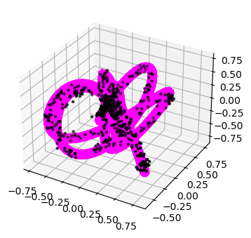
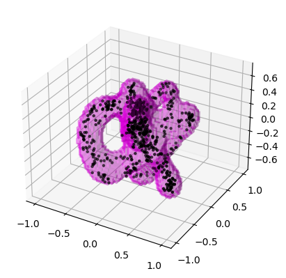
Figure 5: The input point cloud in black, the estimated orbit $\widehat{\mathcal{O}}_{x}$ in magenta (left), and a sublevel set of a kernel density estimator on $\mu_{\widehat{\mathcal{O}}}$ (right).

4.2 The algorithm for $T^{d}$

Employing standard ideas, we describe the set $\mathfrak{orb}(T^{d},n)$ as a direct generalization of $\mathfrak{orb}(\mathrm{SO}(2),n)$. The role of the primitive integral vectors is played by the primitive lattices of $\mathbb{Z}^{n/2}$. We also derive a simplification of Step 3’ in this case.

4.2.1  Orbit-equivalence for $T^{d}$

Let $d\in\mathbb{N}$ positive. As we have seen in Example 2.6, the irreps of the $d$-dimensional torus are parametrized by a weight $\lambda\in\mathbb{Z}^{d}$, where the zero weight corresponds to the trivial representation, and the other irreps have dimension $2$. A representation $\phi$ of $T^{d}$ in $\mathbb{R}^{n}$ can be decomposed into irreps, this decomposition forming a unique multiset $\{\{\lambda_{1},\dots,\lambda_{p}\}\}$ of elements of $\mathbb{Z}^{d}$. As we did for $\mathrm{SO}(2)$, we will suppose that $n$ is even. Moreover, we restrict our discussion to almost-faithful representations, implying that the weights are nonzero, and that $p=n/2$ and $n/2\geq d$. We will denote by $\Lambda(\phi)$ the $(n/2)\times d$ matrix of integers, whose columns are all the nonzero weights in $\{\{\lambda_{1},\dots,\lambda_{p}\}\}$. By renaming the variables, we write the columns as $\Lambda(\phi)=(\lambda_{1},\dots,\lambda_{n/2})$, where the order is chosen arbitrarily. In addition, we will denote by $(\pi_{1},\dots,\pi_{d})$ the rows of $\Lambda(\phi)$, alternatively described as $\pi_{i}=(\lambda_{1}^{i},\dots,\lambda_{n/2}^{i})$ for $i\in[1\dots d]$. By decomposition into irreps, there exists a matrix $O\in\mathrm{SO}(n)$ such that the pushforward Lie algebra $\mathfrak{h}=\mathrm{d}\phi(\mathfrak{g})$ admits the following basis:

$$\big{(}OB(\pi_{1})O^{\top},\dots,OB(\pi_{d})O^{\top}\big{)},$$

and where $B$ as been defined in Equation (16). We stress that this family may not be orthogonal.

We now consider the problem of classification of these representations up to equivalence. Given a representation $\phi$ with weights $\Lambda(\phi)$, we denote by $\langle\Pi(\phi)\rangle$ the corresponding integral lattice, defined as the following discrete subgroup of $\mathbb{R}^{n/2}$:

$$\langle\Pi(\phi)\rangle=\bigg{\{}\sum_{i=1}^{d}\alpha_{i}\pi_{i}\mid(\alpha_{1},\dots,\alpha_{d})\in\mathbb{Z}^{d}\bigg{\}}.$$

Since $\phi$ is almost-faithful, the lattice has rank $d$. It is a sublattice of the integral lattice $\mathbb{Z}^{n/2}$, also known as the weight lattice of the torus $T^{d}$. Their collection will be denoted $\mathcal{R}^{n/2,d}$. Next, let $\phi^{\prime}$ be another representation of $T^{d}$ in $\mathbb{R}^{n}$. Determining whether $\phi$ and $\phi^{\prime}$ are equivalent, based on lattice representations $\langle\Pi(\phi)\rangle$ and $\langle\Pi(\phi^{\prime})\rangle$, is a classical question of representation theory, involving the notions of root systems and Weyl groups. In the case of the torus, the problem is easily solved. Indeed, the representations are equivalent if and only if $\langle\Pi(\phi)\rangle$ can be obtained from $\langle\Pi(\phi^{\prime})\rangle$ via permutation of the axes and reflection along them. By denoting $\mathfrak{S}_{d}\times\{\pm 1\}^{d}$ this group of transformations, we can write the set of equivalence classes of (almost-faithful) representations of $T^{d}$ in $\mathbb{R}^{n}$ as the quotient

$$\mathrm{Rep}(T^{d},\mathbb{R}^{n})\simeq\faktor{\mathcal{R}^{n/2,d}}{\mathfrak{S}_{d}\times\{\pm 1\}^{d}}.$$

Combinatorially, it means that permuting of the columns of $\Pi(\phi)=(\lambda_{1},\dots,\lambda_{n/2})$, or multiplying some of them by $-1$, would yield an equivalent representation.

Next, the question of orbit-equivalence directly follows from the observations above. Indeed, we see that the representations $\phi$ and $\phi^{\prime}$ are orbit-equivalent if and only if one of the lattices $\langle\Pi(\phi)\rangle$ and $\langle\Pi(\phi^{\prime})\rangle$ is included in the other, after a series of permutation of the axes and reflection along them. It is thus natural to consider the primitive lattices of rank $d$, i.e., those sublattices of $\mathbb{Z}^{n/2}$ that are not contained in any larger integral lattice of the same rank. We denote by $\mathcal{R}^{n/2,d}_{\mathrm{prim}}$ their collection. As in the previous paragraph, we deduce a correspondence with the set of orbit-equivalence classes of the torus:

$$\mathrm{OrbRep}(T^{d},\mathbb{R}^{n})\simeq\faktor{\mathcal{R}^{n/2,d}_{\mathrm{prim}}}{\mathfrak{S}_{d}\times\{\pm 1\}^{d}}.$$

In particular, when $d=1$, we recognize the correspondence between $\mathrm{OrbRep}(\mathrm{SO}(2),n)$ and $\mathbb{N}^{n/2}_{\mathrm{prim}}$. Besides, we note that when $n/2=d$, there is only one primitive lattice: $\mathbb{Z}^{d}$ itself.

We mention, as a remark, that the set of primitive lattices $\mathcal{R}^{n/2,d}_{\mathrm{prim}}$ enjoys a similar equidistribution property than the primitive vectors. In order to state this result, let us denote, for any integral lattice $L\subset\mathbb{R}^{n/2,d}$, the space it spans as $V_{L}$. It is a linear subspace of $\mathbb{R}^{n/2}$, that we see as an element of $\mathcal{G}(d,n/2)$, the Grassmannian of $d$-dimensional planes of $\mathbb{R}^{n/2}$. We also denote by $d(L)$ the covolume of $L$, that is, the $d$-dimensional volume of a fundamental region, seen in the subspace $V_{L}$. As it has been shown, for instance in [75, 49], the sequence of sets

$$\big{\{}V_{L}\mid L\in\mathcal{R}^{n/2,d}_{\mathrm{prim}},~{}d(L)\leq r\big{\}}$$

equidistribute, when $r\to\infty$, to the uniform measure on $\mathcal{G}(d,n/2)$. Besides, we remind the reader that, in order to apply our algorithm, one must input a finite subset of $\mathfrak{orb}(T^{d},n)$, the Lie algebras of a set of representatives of orbit-equivalence classes. To do so, we choose a positive integer $\omega_{\mathrm{max}}$, and define $\mathfrak{orb}(T^{d},n,\omega_{\mathrm{max}})$ as those coming from representations with weights at most $\omega_{\mathrm{max}}$. The equidistribution property shows that it is an ‘accurate’ sample of $\mathfrak{orb}(T^{d},n)$.

In practice, the set $\mathcal{R}^{n/2,d}_{\mathrm{prim}}$ can be generated as follows: we first consider the set of all $(n/2)\times d$ matrices with integer coefficients of absolute value at most $\omega_{\mathrm{max}}$, then discard those who do not span a primitive rank lattice of rank $d$, and finally discard matrices when they span the same linear subspace. These conditions are easily verified via algebraic manipulations of their Smith normal form. In our case, however, lattices must be considered up to the action of $\mathfrak{S}_{d}\times\{\pm 1\}^{d}$. To do so, we simply associate to any lattice $L\in\mathcal{R}^{n/2,d}_{\mathrm{prim}}$ the collection of the $n!\times 2^{d}$ spaces $V_{L}$ obtained from it spans, after permutation and reflection of the axes. Another lattice $L^{\prime}$ will define an orbit-equivalent representation if these collections agree. We point out that, although yielding accurately the set $\mathfrak{orb}(T^{d},n,\omega_{\mathrm{max}})$, this procedure is arguably time and memory-consuming, and we expect that improvements could be defined.

4.2.2  Reformulation of Step 3’

We now inspect Step 3’ in the context of $G=T^{d}$. Let $A_{1},\dots,A_{d}$ be eigenvectors associated with the bottom $d$ eigenvalues of the Lie-PCA operator, as given by Step 2, that we skew-symmetrize if they are not, and orthonormalize. We suppose that, after this operation, they still form a free family, i.e., $\langle A_{1},\dots,A_{d}\rangle$ has dimension $d$. We see it as a point of the Grassmannian $\mathcal{G}(d,\mathfrak{so}(n))$ of $d$-planes of $\mathfrak{so}(n)$. The projection matrix

$$\Pi\big{[}\langle A_{1},\dots,A_{d}\rangle\big{]}$$

has dimension $n(n-1)/2\times n(n-1)/2$. Besides, for any lattice $L\in\mathcal{R}^{n/2,d}_{\mathrm{prim}}$, we consider an orthonormal basis $\pi_{1},\dots,\pi_{d}$ of its span, and build the skew-symmetric matrices $B(\pi_{i})=\mathrm{diag}(B(\pi_{i}^{k}))_{k=1}^{n/2}$ for all $j\in[1\dots n/2]$, where $B$ as been defined in Equation (16). We denote their span as $\mathcal{B}=\langle B(\pi_{1}),\dots,B(\pi_{d})\rangle$. Given a matrix $O\in\mathrm{O}(n)$, we consider the conjugated space $O\mathcal{B}O^{\top}$. With these notations, Equation (10) can be written as:

$$\arg\min\big{\|}\Pi\big{[}\langle A_{1},\dots,A_{d}\rangle\big{]}-\Pi\big{[}\langle OB(\pi_{1})O^{\top},\dots,OB(\pi_{d})O^{\top}\rangle\big{]}\big{\|}^{2}\;\;\;\text{s.t. }\begin{cases}L\in\mathcal{R}^{n/2,d}_{\mathrm{prim}},\\ O\in\mathrm{O}(n).\end{cases}$$ (20)

Using Lemma 2.9, we can reformulate it as

$$2\sum_{i=1}^{d}\bigg{(}1-\big{\|}\Pi\big{[}\mathcal{B}\big{]}(OA_{i}O^{\top})\big{\|}^{2}\bigg{)}.$$

In order to study this equation further, let us denote by $\mathcal{C}$ the subspace of $\mathfrak{so}(n)$ spanned by the $(2\times 2)$-block-diagonal skew-symmetric matrices. In particular, $\mathcal{B}$ is a linear subspace of $\mathcal{C}$. We see that, in order to minimize the previous equation, the matrices $O$ must also minimize

$$O\mapsto 2\sum_{i=1}^{d}\big{\|}\Pi\big{[}\mathcal{C}^{\bot}\big{]}(OA_{i}O^{\top})\big{\|}^{2}.$$ (21)

We recognize the problem of simultaneous reduction of a $d$-tuple of skew-symmetric matrices. When the $A_{i}$’s commute, this problem is solved by simply reducing each matrix to its normal form. When they do not, the usual closed-form reduction algorithms cannot be used, and optimization-based methods have been proposed [70, 63]. We will employ the first article: Equation (21) is minimized by a direct optimization on $\mathrm{O}(n)$ via projected gradient descent.

Let $O_{*}$ be a matrix that minimizes the equation. For each $i\in[1\dots d]$, the matrices $\Pi\big{[}\mathcal{C}^{\bot}\big{]}(O_{*}A_{i}O^{\top}_{*})$ takes the form $B(\rho_{i})$ for some $\rho_{i}\in\mathbb{R}^{n/2}$. The collection of the $\rho_{i}$’s span a rank $d$ lattice in $\mathbb{R}^{n/2}$. As a consequence, we see that Equation (20) is nothing but a distance between the lattices $\langle\rho_{i}\rangle_{i=1}^{d}$ and $\langle\pi_{i}\rangle_{i=1}^{d}$. We obtain a direct generalization of Lemma 4.1.

Lemma 4.4.

Suppose that $G=T^{d}$, $n$ is even, and denote by $(\rho_{i})_{i=1}^{d}$ the coefficients of an optimal simultaneous reduction of the matrices $(A_{i})_{i=1}^{d}$. Then Equation (10) is equivalent to

$$\underset{L\in\mathcal{R}_{d}^{n/2}}{\mathrm{arg~{}min}}\sum_{k=1}^{d}f\bigg{(}(\rho_{i}^{k})_{i=1}^{n/2},~{}(\pi_{i}^{k})_{i=1}^{n/2}\bigg{)},$$ (22)

where $f(x,y)=\big{\|}x/\|x\|-y/\|y\|\big{\|}^{2}$, and where $\langle\pi_{i}\rangle_{i=1}^{d}$ denotes any basis of the lattice $L$.

As it was the case for $\mathrm{SO}(2)$, we see that the minimizer of Equation (22) is ill-defined when $(\rho_{i})_{i=1}^{d}$ is not a rational point of the Grassmannian. However, this won’t make any difference in the application of our algorithm, since we restrict the lattices to those admitting a basis with coordinates upper bounded by the parameter $\omega_{\mathrm{max}}$. We have observed that this new formulation of Step 3’ allows for an extreme reduction in computation time. We provide two examples below, consisting of a representation of $T^{2}$ in $\mathbb{R}^{6}$ and one of $T^{3}$ in $\mathbb{R}^{8}$.

Example 4.5.

Figure 6 shows a uniform $750$-sample from an orbit of the representation $\phi_{(1,1)}\oplus\phi_{(1,2)}\oplus\phi_{(2,1)}$ of $T^{2}$ in $\mathbb{R}^{6}$, to which we apply Algorithm 3.1. Besides, we represent the eigenvalues of the Lie-PCA operator. We identify on this graph two significantly small eigenvalues, in accordance with the dimension of the symmetry group. We apply Step 3’, with the formulation of Equation (22), on the $18$ almost-faithful representations of $T^{2}$ in $\mathbb{R}^{6}$ up to orbit-equivalence, that we encode as a $2\times 3$ matrix. We indicate the best twelve values in the table below. The algorithm’s output is $\left(\begin{smallmatrix}0&1&1\\ 2&-2&1\end{smallmatrix}\right)$, that is, the representation $\phi_{(0,2)}\oplus\phi_{(1,-2)}\oplus\phi_{(1,1)}$, which is indeed orbit-equivalent to the original one. Step 4 yields the approximation $\mathrm{d}_{\mathrm{H}}\big{(}X|\widehat{\mathcal{O}}_{x}\big{)}\approx 0.071$, indicating a strong accordance between the input point cloud and the output orbit. As pointed out in Section 3.5.1, this approximation is obtained by sampling $K$ points on $\widehat{\mathcal{O}}_{x}$, with $K$ large, and calculating the Hausdorff distance between the finite point clouds. The bottom right graph of Figure 6 indicates the values of this approximation, for $K$ varying between $10$ and $80^{\prime}000$.

Type	$\left(\begin{smallmatrix}0&1&1\\ 2&-2&1\end{smallmatrix}\right)$	$\left(\begin{smallmatrix}1&1&2\\ -2&2&-1\end{smallmatrix}\right)$	$\left(\begin{smallmatrix}0&1&2\\ 2&-2&-1\end{smallmatrix}\right)$	$\left(\begin{smallmatrix}0&1&1\\ 1&-2&0\end{smallmatrix}\right)$	$\left(\begin{smallmatrix}0&1&1\\ 1&-2&-1\end{smallmatrix}\right)$	$\left(\begin{smallmatrix}0&1&2\\ 2&-2&1\end{smallmatrix}\right)$
Costs	$0.036$	$0.136$	$0.198$	$0.233$	$0.244$	$0.312$
Type	$\left(\begin{smallmatrix}0&1&2\\ 1&-2&-2\end{smallmatrix}\right)$	$\left(\begin{smallmatrix}0&1&2\\ 1&-2&-1\end{smallmatrix}\right)$	$\left(\begin{smallmatrix}1&2&2\\ -2&-2&1\end{smallmatrix}\right)$	$\left(\begin{smallmatrix}1&1&1\\ -2&-1&2\end{smallmatrix}\right)$	$\left(\begin{smallmatrix}0&1&2\\ 1&-2&0\end{smallmatrix}\right)$	$\left(\begin{smallmatrix}0&1&1\\ 1&-2&1\end{smallmatrix}\right)$
Costs	$0.331$	$0.348$	$0.388$	$0.447$	$0.457$	$0.472$

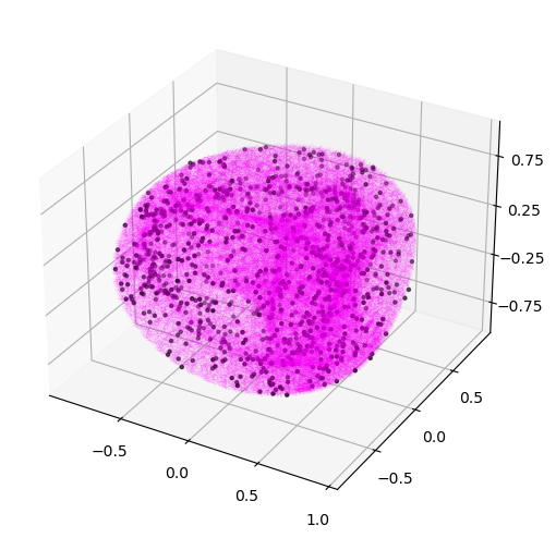
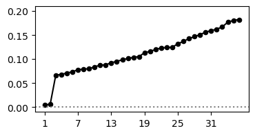
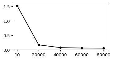
Figure 6: Right: the original point cloud (black) and the estimated orbit (magenta) by Algorithm 3.1. The tight fit suggests that the algorithm converged to the correct representation. Top left: eigenvalues of the Lie-PCA operator, where two small values are identified, corresponding to the dimension of the symmetry group, $T^{2}$. Bottom left: approximation of the Hausdorff distance between the point cloud and the orbit, as the approximation parameter $K$ increases.

Example 4.6.

We apply Algorithm 3.1 to a $1500$-sample an orbit of the representation $\phi_{(-1,0,-1)}\oplus\phi_{(1,0,0)}\oplus\phi_{(1,1,0)}\oplus\phi_{(-1,-1,-1)}$ of $T^{3}$ in $\mathbb{R}^{8}$. There are $10$ non-orbit-equivalent and almost-faithful representations of $T^{3}$ in $\mathbb{R}^{8}$ with weights in $\{-1,0,1\}$. We apply Step 3’ with the formulation of Equation (22) on these representations, and obtain as an output $\phi_{(0,0,1)}\oplus\phi_{(1,0,-1)}\oplus\phi_{(1,-1,-1)}\oplus\phi_{(0,-1,1)}$, which is indeed orbit-equivalent to the initial representation. Step 4 gives the Hausdorff distance $\mathrm{d}_{\mathrm{H}}\big{(}X|\widehat{\mathcal{O}}_{x}\big{)}\approx 0.058$, that we consider as a good fit.

4.3 The algorithm for $\mathrm{SU}(2)$ and $\mathrm{SO}(3)$

We now turn to the two non-Abelian groups of interest in this paper. We show that their notion of orbit-equivalence coincides with that of equivalence. In opposition to $T^{d}$, we did not obtain a simplification of Step 3’. We give several applications of Algorithm 3.1 on synthetic datasets.

4.3.1  Orbit-equivalence for $\mathrm{SU}(2)$

As pointed out in Section 2.2.3, if $G$ denotes a compact Lie group, then for any representation $\phi\colon G\rightarrow\mathrm{GL}_{n}(\mathbb{R})$ and any surjective homomorphism $f\colon G\rightarrow G$, the representation $f\circ\phi$ is orbit-equivalent to $\phi$. In the case of the torus $T^{d}$, these homomorphisms can be identified with $\mathrm{GL}_{d}(\mathbb{R})\cap\mathrm{M}_{d}(\mathbb{Z})$, the $d\times d$ integer matrices with nonzero determinant. This was the idea behind Sections 4.1 and 4.2, where we eventually described $\mathfrak{orb}(T^{d},n)$ as a quotient of the set of lattices. In the case of $\mathrm{SU}(2)$ or $\mathrm{SO}(3)$, however, this analysis is greatly simplified, due to the fact that their surjective homomorphism are automorphisms, which are in turn inner automorphisms.

Lemma 4.7.

Two orbit-equivalent representations of $G=\mathrm{SU}(2)$ or $\mathrm{SO}(3)$ are equivalent.

Proof.

Consider two representations $\phi,\phi^{\prime}\colon G\rightarrow\mathrm{GL}_{n}(\mathbb{R})$, with $\mathfrak{h}=\mathrm{d}\phi(\mathfrak{g})$ and $\mathfrak{h}^{\prime}=\mathrm{d}\phi^{\prime}(\mathfrak{g})$ their pushforward Lie algebras. We suppose that $\phi$ and $\phi^{\prime}$ are orbit-equivalent, meaning that there exists a matrix $M\in\mathrm{GL}_{n}(\mathbb{R})$ such that $h^{\prime}=M\mathfrak{h}M^{-1}$. In particular, the conjugation by $M$ induces an automorphism of $\mathfrak{h}$, that we denote by $u$. It is a property of the groups $\mathrm{SU}(2)$ and $\mathrm{SO}(3)$ that any automorphism of their Lie algebra comes from an automorphism of the group. That is, there exists an automorphism $f\colon G\rightarrow G$ such that $\mathrm{d}f=u$. This fact can be seen as a consequence of Ado’s theorem [45, Th. 7.4.1]. Moreover, these groups being of type $B_{n}$ in Dynkin diagram’s classification of Lie algebras, we know that their automorphisms are all inner automorphisms. In other words, there exists $g\in G$ such that $\forall h\in G,f(h)=ghg^{-1}$. The matrix $M^{\prime}=\phi(g)\in\mathrm{GL}_{n}(\mathbb{R})$ provides an equivalence between the representations $\phi$ and $\phi^{\prime}$. ∎

We are left with describing explicitly the set of equivalence classes of representations. Let us start with the group $\mathrm{SU}(2)$. Referring to Example 2.7, it admits one irrep in $\mathbb{R}^{k}$ for each $k\geq 1$ such that $k\equiv 1\pmod{2}$ or $k\equiv 0\pmod{4}$. We denote the corresponding representation by $\phi_{k}$. We deduce that the equivalence classes of representations of $\mathrm{SU}(2)$ in $\mathbb{R}^{n}$ are given by the partitions of $n$ into integers in $(2\mathbb{N}+1)\cup 4\mathbb{N}$. Let us denote this set as $\mathrm{Part}\big{(}n,(2\mathbb{N}+1)\cup 4\mathbb{N}\big{)}$. By denoting $B(k)=(B(k)_{1},B(k)_{2},B(k)_{3})$ the basis of the pushforward Lie Algebra of $\phi_{k}$ given in Appendix A.2.2, we obtain the explicit description

$$\mathfrak{orb}(\mathrm{SU}(2),n)=\big{\{}\big{(}B(k_{1}),\dots,B(k_{p})\big{)}\mid(k_{1},\dots,k_{p})\in\mathrm{Part}\big{(}n,(2\mathbb{N}+1)\cup 4\mathbb{N}\big{)}\big{\}}.$$

In the case of $\mathrm{SO}(3)$, only the irreps with $k=1$ or $k\equiv 0\pmod{4}$ are considered, yielding

$$\mathfrak{orb}(\mathrm{SO}(3),n)=\big{\{}\big{(}B(k_{1}),\dots,B(k_{p})\big{)}\mid(k_{1},\dots,k_{p})\in\mathrm{Part}\big{(}n,2\mathbb{N}+1\big{)}\big{\}}.~{}~{}~{}~{}~{}~{}~{}~{}~{}~{}$$

We note that the cardinal of both these sets is lower than the number of partitions of the integer $n$, that we know is equivalent to $\exp(\pi\sqrt{2n/3})/(4\sqrt{3}n)$. Moreover, these set being finite, we do not have to restrict them to $\omega_{\mathrm{max}}$, as we did for $\mathfrak{orb}(\mathrm{SO}(2),n,\omega_{\mathrm{max}})$ and $\mathfrak{orb}(T^{d},n,\omega_{\mathrm{max}})$.

4.3.2  Application of the algorithm

As described above, the classes of orbit-equivalent representations of $\mathrm{SU}(2)$ and $\mathrm{SO}(3)$ are given by the partitions of the integer $n$, respectively with odd terms and multiples of four, and only odd terms. In practice, these partitions are easily computed, for instance using the algorithm of [53]. Step 3 of Algorithm 3.1 is put in practice by parsing this list of partitions. This is illustrated in the seven examples below, for representations in the Euclidean space $\mathbb{R}^{n}$ with $n=5,7,11,6,8,9$ and $16$.

Example 4.8.

Using the explicit formulae for irreps of $\mathfrak{so}(3)$ in Appendix A.2.2, we apply the algorithm for the data $X$ of $1500$ points created from an orbit of the irreducible representation of $\mathrm{SO}(3)$ in $\mathbb{R}^{5}$. Namely, the pushforward Lie algebra is spanned by

$$\left(\begin{matrix}0&0&0&-1&0\\ 0&0&1&0&0\\ 0&-1&0&0&0\\ 1&0&0&0&-\sqrt{3}\\ 0&0&0&\sqrt{3}&0\end{matrix}\right),~{}~{}~{}\left(\begin{matrix}0&0&1&0&0\\ 0&0&0&1&0\\ -1&0&0&0&-\sqrt{3}\\ 0&-1&0&0&0\\ 0&0&\sqrt{3}&0&0\end{matrix}\right),~{}~{}~{}\mathrm{and}~{}~{}~{}\left(\begin{matrix}0&-2&0&0&0\\ 2&0&0&0&0\\ 0&0&0&-1&0\\ 0&0&1&0&0\\ 0&0&0&0&0\end{matrix}\right).$$

The left side of Figure 7 indicates the result of spectral analysis applied to this data, which makes it clear that a three-dimensional Lie algebra generates it, making $\mathfrak{su}(2)$ a good candidate. Through Step 3, we found that the three non-trivial representations of $\mathrm{SU}(2)$ in $\mathbb{R}^{5}$, associated to the partitions $(5)$, $(1,1,3)$ and $(3,4)$, have respective cost $0.001$, $0.011$ and $0.015$, confirming that the point cloud has been sampled on the irrep of $\mathrm{SO}(3)$. Through Step 4, we obtain the distance $\mathrm{d}_{\mathrm{H}}\big{(}X|\widehat{\mathcal{O}}_{x}\big{)}\approx 0.088$, evidence of a successful run of the algorithm. We give the graph of the estimated Hausdorff distances for different sample sizes on the right side of Figure 7.

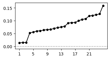
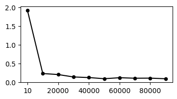
Figure 7: Left: eigenvalues of the Lie-PCA operator. Right: estimated Hausdorff distance $\mathrm{d}_{\mathrm{H}}\big{(}X|\widehat{\mathcal{O}}_{x}\big{)}$ for varying numbers of samples.

Example 4.9.

The non-trivial representations of $\mathrm{SU}(2)$ in $\mathbb{R}^{7}$ are given by the partitions

$$(1,1,1,1,3),~{}(1,1,1,4),~{}(1,1,5),~{}(1,3,3),~{}(3,4)~{}\mathrm{and}~{}(7).$$

Only the last two representations yield orbits which span the ambient space $\mathbb{R}^{7}$. We sample $3000$ points on them, denote the point clouds $X_{(3,4)}$, and $X_{(7)}$, and run Algorithm 3.1. The Lie-PCA operator, in Figure 8, exhibits respectively four and three small eigenvalues. According to the results of Step 3 in the following table, the algorithm has succeeded in identifying the representations. Step 4 yiels estimated orbits for $X_{(3,4)}$ and $X_{(7)}$ with Hausdorff distances approximately $0.032$ and $0.096$. These values can be considered as small, as seen in Figure 9.

Representation	$(1,1,1,1,3)$	$(1,1,1,4)$	$(1,1,5)$	$(1,3,3)$	$(3,4)$	$(7)$
Cost for $X_{(3,4)}$	$0.016$	$0.012$	$0.012$	$0.012$	$4\times 10^{-5}$	$0.013$
Cost for $X_{(7)}$	$0.027$	$0.029$	$0.026$	$0.027$	$0.027$	$0.025$

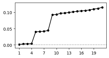
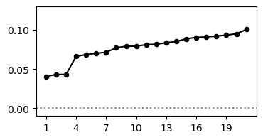
Figure 8: Eigenvalues of Lie-PCA operator on the orbits of the representations $(3.4)$ and $(7)$ of $\mathrm{SU}(2)$ in $\mathbb{R}^{7}$, restricted to the skew-symmetric matrices for visualization ease.

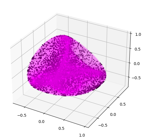
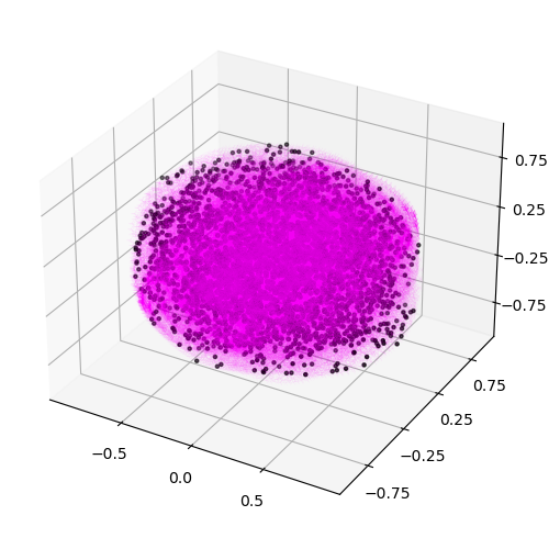
Figure 9: Left: a sample of an orbit of the representation $(3,4)$ of $\mathrm{SU}(2)$ in $\mathbb{R}^{7}$ (black) and the estimated orbit by Algorithm 3.1 (magenta). Right: same for the representation of partition $(7)$.

Example 4.10.

We reproduce Example 4.9, now in $\mathbb{R}^{11}$. The representations of $\mathrm{SU}(2)$ are given by the following admissible partitions of $11$, where we omit the $1$’s:

$$(3),~{}(4),~{}(5),~{}(3,3),~{}(3,4),~{}(7),~{}(3,5),~{}(4,4),~{}(8),~{}(3,3,3),~{}(4,5),~{}$$

$$(9),~{}(3,3,4),~{}(3,7),~{}(5,5),~{}(3,3,5),~{}(3,4,4),~{}(3,8),~{}(4,7),~{}~{}\mathrm{and}~{}(11).$$

We sample $5000$ points on orbits of the last three representations. In each case, Algorithm 3.1 outputs the correct representation, with Hausdorff distances respectively $0.077$, $0.107$ and $0.184$. Repeating the same experiment with drawing only $3000$ points yields $0.122$, $0.182$ and $0.239$.

Example 4.11.

Let $\mathcal{O}$ be the set of $2\times 3$ matrices with orthonormal rows, embedded in $\mathbb{R}^{6}$ by flattening. We create a set $X$ of $3000$ points uniformly sampled on $\mathcal{O}$, on which we apply Algorithm 3.1. Through Step 1, we observe that the covariance matrix of $X$ has eigenvalues between $0.159$ and $0.174$, hence we do not perform dimension reduction. The Lie-PCA operator, computed in Step 2, presents four significantly small eigenvalues. Among the four non-trivial representations of $\mathrm{SU}(2)$ in $\mathbb{R}^{6}$, Step 3 detects the partition $(3,3)$ as that yielding the minimal cost. It corresponds to a representation of $\mathrm{SO}(3)$. Finally, Step 4 outputs the distance $\mathrm{d}_{\mathrm{H}}\big{(}X|\widehat{\mathcal{O}}_{x}\big{)}\approx 0.091$, witnessing a good fit between the point cloud and the estimated orbit. These results are coherent with the fact that the initial set $\mathcal{O}$ is indeed an orbit of a representation of $\mathrm{SO}(3)$ in $\mathbb{R}^{6}$, namely, that coming from the action of $\mathrm{SO}(3)$ on $\mathrm{M}_{2,3}(\mathbb{R})$ by simultaneous multiplication of the rows. The orbit is the Stiefel manifold $\mathcal{V}(2,\mathbb{R}^{3})$, homeomorphic to $\mathrm{SO}(3)$.

Example 4.12.

We reproduce Example 4.11 in higher dimension: $\mathcal{O}$ now is the Stiefel manifold $\mathcal{V}(2,\mathbb{R}^{4})$ seen in $\mathrm{M}_{2,4}(\mathbb{R})$, i.e., it is the $2\times 3$ matrices with orthonormal rows. It carries a transitive action of $\mathrm{SO}(4)$. We generate a $10^{\prime}000$-sample $X$. By applying Algorithm 3.1 with $G=\mathrm{SO}(3)$, we expect to identify a sub-action induced by an inclusion $\mathrm{SO}(3)\hookrightarrow\mathrm{SO}(4)$. Up to orbit-equivalence, this group admits five distinct non-trivial representations in $\mathbb{R}^{8}$, indexed by

$$(1,1,1,1,1,3),~{}(1,1,1,5),~{}(1,7),~{}(1,1,3,3)~{}~{}\mathrm{and}~{}~{}(3,5).$$

Step 3 recognizes $(1,1,3,3)$ as the optimal representation. By choosing an arbitrary point $x\in X$, Step 4 yields the distance $\mathrm{d}_{\mathrm{H}}\big{(}X|\widehat{\mathcal{O}}_{x}\big{)}\approx 1.838$, showing that the orbit do not approximate $X$ correctly. The opposite Hausdorff distance, however, is small: $\mathrm{d}_{\mathrm{H}}\big{(}\widehat{\mathcal{O}}_{x}|X\big{)}\approx 0.571$. This suggests that we have generated a subset of $\mathcal{O}$. In order to verify this statement, we generate the set $\widehat{\mathcal{O}}=\{\widehat{\mathcal{O}}_{x}\mid x\in X\}$. The fitting is now correct: $\mathrm{d}_{\mathrm{H}}\big{(}X|\widehat{\mathcal{O}}\big{)}=0$ and $\mathrm{d}_{\mathrm{H}}\big{(}\widehat{\mathcal{O}}|X\big{)}\approx 0.642$. We deduce that the estimated action is not transitive.

Example 4.13.

In the same vein as Examples 4.11 and 4.12, let $\mathcal{O}$ be the $3\times 3$ special orthogonal matrices, embedded in $\mathbb{R}^{9}$, and $X$ a $3000$-sample. Since $\mathrm{SO}(3)$ acts transitively on itself, $\mathcal{O}$ can be seen as an orbit of it. While running Algorithm 3.1, Step 2 shows a Lie-PCA operator with six almost-zero eigenvalues. This coincides with the dimension of the isometry group of $\mathrm{SO}(3)$ given in Section 2.1.4, equal to $\mathrm{SO}(3)\rtimes\mathrm{SO}(3)\times\{\pm 1\}$. Among the twelve non-trivial representations of $\mathrm{SU}(2)$ in $\mathbb{R}^{9}$, Step 3 yields the following costs, where we omit the $1$’s in the partitions:

Representation	$(3,5)$	$(3,3,3)$	$(4,5)$	$(8)$	$(5)$	$(7)$
Cost	$2\times 10^{-5}$	$4\times 10^{-5}$	$0.001$	$0.001$	$0.03$	$0.004$
Representation	$(9)$	$(3,3)$	$(3,4)$	$(4,4)$	$(3)$	$(4)$
Cost	$0.004$	$0.006$	$0.007$	$0.009$	$0.011$	$0.013$

The optimum is given by the partition $(3,5)$. However, this Lie algebra does not seem to generate $X$: the Hausdorff distance, equal to $\mathrm{d}_{\mathrm{H}}\big{(}X|\widehat{\mathcal{O}}_{x}\big{)}\approx 2.658$, is large. In comparison, the distance from the orbit to $X$ is small: $\mathrm{d}_{\mathrm{H}}\big{(}\widehat{\mathcal{O}}_{x}|X\big{)}\approx 0.543$. This indicates that the representation $(3,5)$ yields an orbit that is only a subset of $\mathcal{O}$. As seen in the previous table, another good candidate is the representation $(3,3,3)$. We run Step 4 again, now using the optimal Lie algebra computed for this latter representation. The set $X$ is now well approached, since $\mathrm{d}_{\mathrm{H}}\big{(}X|\widehat{\mathcal{O}}_{x}\big{)}\approx 0.061$.

Example 4.14.

For our last example, we consider the embedding $\mathcal{G}(2,\mathbb{R}^{4})\hookrightarrow\mathbb{R}^{4\times 4}$ of the Grassmann manifold into the Euclidean space via projection matrices, and sample $5000$ points on it. Just as it was the case for the Stiefel manifold $\mathcal{V}(2,\mathbb{R}^{4})$ in Example 4.12, the group $\mathrm{SO}(4)$ acts transitively on $\mathcal{G}(2,\mathbb{R}^{4})$. By applying Algorithm 3.1 with $G=\mathrm{SO}(3)$, we identify $(1,3,5)$ as the optimal representation. Instead of computing $\widehat{\mathcal{O}}_{x}$ for a certain data point $x$, we consider their union $\widehat{\mathcal{O}}$. We eventually get $\mathrm{d}_{\mathrm{H}}\big{(}X|\widehat{\mathcal{O}}\big{)}=0$ and $\mathrm{d}_{\mathrm{H}}\big{(}\widehat{\mathcal{O}}|X\big{)}\approx 0.453$, showing a good fit.

5 Theoretical guarantees

In this section, we derive theoretical results regarding Algorithm 3.1, guaranteeing that the output $\widehat{\mathcal{O}}_{x}$ will be close to the underlying orbit $\mathcal{O}$. The quality of these results depends on the proximity of the input $X$ to the orbit $\mathcal{O}$. In the literature, two common measures of this proximity are the Hausdorff distance $\mathrm{d}_{\mathrm{H}}\big{(}X,\mathcal{O}\big{)}$ and the Wasserstein distance $\mathrm{W}_{2}(\mu_{X},\mu_{\mathcal{O}})$ (defined in Sections 3.5.1 and 3.5.2). Here, $\mu_{X}$ and $\mu_{\mathcal{O}}$ are measures associated with $X$ and $\mathcal{O}$, typically the empirical and uniform measures. We found that the Wasserstein distance is better suited to analyse our algorithm. Indeed, at its core is performed an estimation of normal spaces via local PCA. Such an operation is stable with respect to the Wasserstein, but not the Hausdorff distance.

Certain results of this section are stated for arbitrary probability measures $\mu$ and $\nu$ on $\mathbb{R}^{n}$, and others hold only with additional assumptions. In order to ensure clarity, the notation $\mu_{X}$ will denote exclusively the empirical measure on $X$, and $\mu_{\mathcal{O}}$ the uniform measure on $\mathcal{O}$. As recalled in Section 2.1.3, $\mu_{\mathcal{O}}$ can be seen as a pushforward of the Haar measure $\mu_{G}$, or, equivalently, as the restriction of the $l$-dimensional Hausdorff measure to it, where $l$ is its dimension.

Our investigation is organized as follows. In Section 5.1, we raise the issue of dimensionality reduction with PCA, in the context of Lie group orbits. Next, we analyse Lie-PCA in Section 5.2. We gather in Section 5.3 guarantees regarding the minimization problems involved in the algorithm. These results are brought together in Section 5.4, giving Theorem 5.21.

5.1 PCA and orthonormalization

As a general practice in data analysis, is it common to apply dimension reduction to the dataset $X$, allowing to reduce the computational cost of the algorithms to come. In our context, applying dimension reduction does not only allow to speed up our algorithm, it is also a crucial procedure for ensuring its consistency, as we will explain in Remark 5.20. However, not any dimension reduction algorithm can be used: supposing that the dataset $X$ lies on or close an orbit $\mathcal{O}$ of a representation of a Lie group $G$, we must ensure that the projected dataset still does. In this section, we will show how to project $X$ into $\langle\mathcal{O}\rangle$, the linear subspace spanned by $\mathcal{O}$, via the common method of PCA. More generally, one may wish to reduce the dimension further. The particular case of $G=\mathrm{SO}(2)$ and $T^{d}$ will be treated in Section 6.1.

Such a pre-processing step intervenes a second time in Step 1, where the points are normalized, so as to transform the representation into an orthogonal one. This step, as well as the PCA, involves the computation of the covariance matrix of $X$. In order to prove stability results with respect to the Wasserstein distance, we should use a definition of it adapted to measures. In this regard, we define the covariance matrix of a square-integrable measure $\mu$ on $\mathbb{R}^{n}$ as

$$\Sigma[\mu]=\int xx^{\top}\mathrm{d}\mu(x)=\int\|x\|^{2}\Pi\big{[}\langle x\rangle\big{]}\mathrm{d}\mu(x),$$ (23)

where $xx^{\top}$ represents the tensor product of the vector $x$ by itself, which is equal to the projection $\Pi\big{[}\langle x\rangle\big{]}$ when $x$ has norm $1$. This integral is a symmetric $n\times n$ matrix, hence diagonalizable. Given an integer $m$, PCA refers to the projection operator on any $m$ top eigenvectors of $\Sigma[\mu]$, that is, eigenvectors associated with the $m$ largest eigenvalues. It is denoted $\Pi^{m}_{\Sigma(\mu)}$. When $\mu$ is $\mu_{X}$, the empirical measure on a finite point cloud, we recover the usual definition of PCA.

We divide our analysis in two. Section 5.1.1 gathers results regarding covariance matrices, and applies them in the context of PCA. The same tools are employed in Section 5.1.2 to the problem of orthonormalization. We stress that the ideas developed in this section are not new; the originality lies in the effort to obtain explicit bounds, in terms of the Wasserstein distance.

5.1.1  Analysis of PCA

Our strategy to study the covariance matrix of $X$ consists in comparing it to $\Sigma[\mu_{\mathcal{O}}]$, the covariance of the orbit $\mathcal{O}$, that we consider as the ‘ideal’ case. Let $\phi\colon G\rightarrow\mathrm{M}_{n}(\mathbb{R})$ be a representation that generates the orbit. Let also $x_{0}\in\mathcal{O}$ an arbitrary point, that is fixed throughout this section. Any other point $x\in\mathcal{O}$ can be written $x=\phi(g)x_{0}$ for some $g\in G$. Using that $\mu_{\mathcal{O}}$ is the pushforward of the Haar measure $\mu_{G}$ on $G$, Equation (23) reads

$$\Sigma[\mu_{\mathcal{O}}]=\int\big{(}\phi(g)x_{0}\big{)}\cdot\big{(}\phi(g)x_{0}\big{)}^{\top}\mathrm{d}\mu_{G}(g).$$

We observe that its trace is equal to the moment of order two of $\|\mu_{\mathcal{O}}\|$:

$$\operatorname{tr}\big{(}\Sigma[\mu_{\mathcal{O}}]\big{)}=\int\operatorname{tr}\big{(}\big{(}\phi(g)x_{0}\big{)}\cdot\big{(}\phi(g)x_{0}\big{)}^{\top}\big{)}\mathrm{d}\mu_{G}(g)=\int\big{\|}\phi(g)x_{0}\big{\|}^{2}\mathrm{d}\mu_{G}(g)=\mathbb{E}[\|\mu_{\mathcal{O}}\|^{2}].$$ (24)

Now, let $\mathbb{R}^{n}=\bigoplus_{i=1}^{m}V_{i}$ be the decomposition of $\phi$ into irreps, and denote as $(\Pi\big{[}V_{i}\big{]})_{i=1}^{m}$ the projection matrices on these subspaces. We can decompose the previous equality in

$$\Sigma[\mu_{\mathcal{O}}]=\sum_{i=1}^{m}\underbrace{\int\phi_{i}(g)\bigg{(}\Pi\big{[}V_{i}\big{]}(x_{0})\cdot\Pi\big{[}V_{i}\big{]}(x_{0})^{\top}\bigg{)}\phi_{i}(g)^{\top}\mathrm{d}\mu_{G}(g)}_{C_{i}}.$$

Each $C_{i}$ is a symmetric matrix and is zero on the $V_{j}$’s for which $j\neq i$. Moreover, $C_{i}$ is zero if and only if $\Pi\big{[}V_{i}\big{]}(x_{0})=0$. We deduce that the kernel of $\Sigma[\mu_{\mathcal{O}}]$ is $\langle\mathcal{O}\rangle^{\bot}$. We now suppose that $\phi$ is orthogonal. In particular, $g\mapsto\|\phi(g)x_{0}\|$ is constant. We deduce that the variance $\mathbb{V}[\|\mu_{\mathcal{O}}\|]$ is zero, and that $\operatorname{tr}(\Sigma[\mu_{\mathcal{O}}])=\|x_{0}\|^{2}$. Besides, by Schur’s lemma, the $C_{i}$ are homotheties:

$$\Sigma[\mu_{\mathcal{O}}]=\sum_{i=1}^{m}\sigma_{i}^{2}\Pi\big{[}V_{i}\big{]}~{}~{}~{}~{}~{}~{}\mathrm{where}~{}~{}~{}~{}~{}\sigma_{i}^{2}=\frac{1}{\dim(V_{i})}\int\big{\|}\Pi\big{[}V_{i}\big{]}(x)\big{\|}^{2}\mathrm{d}\mu_{\mathcal{O}}(x)=\frac{\big{\|}\Pi\big{[}V_{i}\big{]}(x_{0})\big{\|}^{2}}{\dim(V_{i})}.$$

Note that, without further assumptions, the eigenvalues $(\sigma_{i}^{2})_{i=1}^{m}$ can be any vector of positive coordinates whose sum is $\|x_{0}\|^{2}$. In what follows, we will call homogeneous an orbit of an orthogonal representation whose eigenvalues are all equal. We see it as the most ‘regular’ orbit.

In this section, we do not make the hypothesis that the representation is orthogonal, but we deduce from this discussion that two quantities are naturally involved in the problem:

• The variance $\mathbb{V}[\|\mu_{\mathcal{O}}\|]$, which we see as a measure of deviation from orthogonality of $\mathcal{O}$. When the representation is orthogonal, it is zero.

• The ratio $\sigma_{\mathrm{max}}^{2}/\sigma_{\mathrm{min}}^{2}$ between the top and bottom nonzero eigenvalue of $\Sigma[\mu_{\mathcal{O}}]$, understood as a measure of homogeneity of $\mathcal{O}$. When the orbit is homogeneous, it is one.

The ideal case having been treated, we now turn to $X$. In order to study how accurately $\Sigma[\mu_{\mathcal{O}}]$ can be approximated by $\Sigma[\mu_{X}]$, we give a general stability result for covariance matrices. Combined with Davis-Kahan theorem (Lemma 5.3), we will deduce Proposition 5.4. We stress that the results to follow do not involve the hypothesis that the measure $\mu_{X}$ comes from a point cloud. Instead, we work in the broader setting of an arbitrary probability measure $\nu$.

Lemma 5.1.

For any two square-integrable measures $\mu$ and $\nu$ on $\mathbb{R}^{n}$, we have

$$\|\Sigma[\mu]-\Sigma[\nu]\|_{\mathrm{F}}\leq\big{(}2\mathbb{V}[\|\mu\|]^{1/2}+\mathrm{W}_{2}(\mu,\nu)\big{)}\mathrm{W}_{2}(\mu,\nu).$$

Proof.

Let $\pi$ and optimal transport plan for the Wasserstein distance $\mathrm{W}_{2}(\mu,\nu)$. We write

$$\|\Sigma[\mu]-\Sigma[\nu]\|_{\mathrm{F}} \leq\int\|xx^{\top}-yy^{\top}\|\mathrm{d}\pi(x,y)$$

$$\leq\int(\|x\|+\|y\|)\|x-y\|\mathrm{d}\pi(x,y)$$

$$\leq\sqrt{\int(\|x\|+\|y\|)^{2}\mathrm{d}\pi(x,y)}\cdot\sqrt{\int\|x-y\|^{2}\mathrm{d}\pi(x,y)},$$

where the second line follows from Lemma 5.2 stated below, and the last line from Hölder’s inequality. The second term of the product is equal to $\mathrm{W}_{2}(\mu,\nu)$. Concerning the first term, we introduce the quantity $\mathbb{E}[\|\mu\|]$ and use the subadditivity of the $L^{2}$-norm:

$$\sqrt{\int(\|x\|+\|y\|)^{2}\mathrm{d}\pi(x,y)} \leq\sqrt{\int(\|x\|-\mathbb{E}[\|\mu\|])^{2}\mathrm{d}\pi(x,y)}+\sqrt{\int(\|y\|-\mathbb{E}[\|\mu\|])^{2}\mathrm{d}\pi(x,y)}.$$

The first term of the sum is equal to $\mathbb{V}[\|\mu\|]^{1/2}$. We bound the second one using the triangle inequality $\|y\|-\mathbb{E}[\|\mu\|]\leq(\|x\|-\mathbb{E}[\|\mu\|])+\|y-x\|$ and the subadditivity:

$$\sqrt{\int(\|y\|-\mathbb{E}[\|\mu\|])^{2}\mathrm{d}\pi(x,y)}\leq\sqrt{\int(\|x\|-\mathbb{E}[\|\mu\|])+\|y-x\|])^{2}\mathrm{d}\pi(x,y)}\leq\mathbb{V}[\|\mu\|]^{\frac{1}{2}}+\mathrm{W}_{2}(\mu,\nu).$$

Adding these terms yields the inequality of the lemma. ∎

Lemma 5.2.

For every $x,y\in\mathbb{R}^{n}$, we have $\|xx^{\top}-yy^{\top}\|\leq(\|x\|+\|y\|)\|x-y\|$.

Proof.

The triangle inequality on $xx^{\top}-yy^{\top}=(x-y)x^{\top}+y(x-y)^{\top}$ yields

$$\|xx^{\top}-yy^{\top}\| \leq\|x-y\|\|x\|+\|y\|\|x-y\|=(\|x\|+\|y\|)\|x-y\|.\qed$$

Lemma 5.1 shows that the distance between the covariance matrices of two measures is small, provided that their Wasserstein distance is. We now wish to obtain a similar result for the PCA, that is, the projection matrices on their top eigenspaces. If $U$ and $V$ are linear subspaces of $\mathbb{R}^{n}$, we will quantify their proximity via $\|\Pi\big{[}U\big{]}-\Pi\big{[}V\big{]}\|_{\mathrm{F}}$, the Frobenius norm between their projections, just as we defined in Section 2.3.1 for subspaces of $\mathfrak{so}(n)$. We mention that

$$\|\Pi\big{[}U\big{]}-\Pi\big{[}V\big{]}\|_{\mathrm{F}}=\sqrt{2}\|\sin\Theta(U,V)\|,$$

where $\Theta(U,V)\in\mathbb{R}^{n}$ denotes the principal angles between $U$ and $V$. These are defined recursively, as the minimal angles between two unit vectors of the subspaces (see [25, Sec. 2]).

Now, let $A,B\in\mathrm{M}_{n}(\mathbb{R})$ be two symmetric matrices, $m\in[1\dots n]$ an integer, and $\Pi_{A}^{m},\Pi_{B}^{m}$ the projection matrices on the subspaces of $\mathbb{R}^{n}$ spanned by any top $m$ eigenvectors of $A$ and $B$. The problem of bounding $\|\Pi_{A}^{m}-\Pi_{B}^{m}\|_{\mathrm{F}}$ in terms of $\|A-B\|_{\mathrm{F}}$ is a classical question of matrix perturbation theory. The stability of eigenvalues is given by Weyl’s theorem: for any eigenvalue $\lambda$ of $A$, there exists an eigenvalue $\mu$ of $B$ such that $|\lambda-\mu|\leq\|A-B\|_{\mathrm{F}}$ [81, Cor. VI.4.10]. On the other hand, the stability of eigenspaces is given by Davis-Kahan theorem [25], which we reformulate in the following lemma, and will use on several occasions throughout the rest of this paper. Moreover, for a symmetric matrix in $\mathrm{M}_{n}(\mathbb{R})$ with sorted eigenvalues $\lambda_{1}\geq\dots\geq\lambda_{n}$, and an integer $m\in[1\dots n-1]$, we call $m^{\mathrm{th}}$ eigengap the difference $\lambda_{m}-\lambda_{m+1}$. As a consequence of Weyl’s theorem, if $\delta$ is the $m^{\mathrm{th}}$ eigengap of $A$, then that of $B$ is at least $\delta-2\|A-B\|_{\mathrm{F}}$.

Lemma 5.3.

(Davis-Kahan theorem) Let $A,B\in\mathrm{M}_{n}(\mathbb{R})$ be symmetric matrices, $m\in[1\dots n-1]$ an integer, and $\delta$ the $m^{\mathrm{th}}$ eigengap of $A$. If $\|A-B\|_{\mathrm{F}}<\delta/2$, then

$$\|\Pi_{A}^{m}-\Pi^{m}_{B}\|_{\mathrm{F}}\leq\sqrt{2}/\delta\|A-B\|_{\mathrm{F}}.$$

The result also holds if we consider the bottom eigenvectors instead of the top, or if we consider the operator norm instead of the Frobenius one.

Equipped with these results, we can derive our main proposition concerning PCA.

Proposition 5.4.

Let $\mathcal{O}\subset\mathbb{R}^{n}$ be the orbit of a representation, potentially non-orthogonal, $\mu_{\mathcal{O}}$ its uniform measure, $\Pi\big{[}\langle\mathcal{O}\rangle\big{]}$ the projection on its span, and $\sigma_{\mathrm{max}}^{2},\sigma_{\mathrm{min}}^{2}$ the top and bottom nonzero eigenvalues of $\Sigma[\mu_{\mathcal{O}}]$. Let also $\nu$ be a measure, $\Sigma[\nu]$ its covariance matrix, $\epsilon>0$ and $\Pi_{\Sigma[\nu]}^{>\epsilon}$ the projection on the subspace spanned by eigenvectors of eigenvalue at least $\epsilon$. We suppose

$$\frac{\mathrm{W}_{2}(\mu_{\mathcal{O}},\nu)}{\sigma_{\mathrm{min}}}<\bigg{(}\frac{\mathbb{V}\big{[}\|\mu_{\mathcal{O}}\|\big{]}}{\sigma_{\mathrm{min}}^{2}}+\frac{1}{2}\bigg{)}^{1/2}-\bigg{(}\frac{\mathbb{V}\big{[}\|\mu_{\mathcal{O}}\|\big{]}}{\sigma_{\mathrm{min}}^{2}}\bigg{)}^{1/2}$$

$$\mathrm{and}~{}~{}~{}~{}~{} \bigg{(}2\bigg{(}\frac{\mathbb{V}\big{[}\|\mu_{\mathcal{O}}\|\big{]}}{\sigma_{\mathrm{min}}^{2}}\bigg{)}^{1/2}+\frac{\mathrm{W}_{2}(\mu_{\mathcal{O}},\nu)}{\sigma_{\mathrm{min}}}\bigg{)}\cdot\bigg{(}\frac{\mathrm{W}_{2}(\mu_{\mathcal{O}},\nu)}{\sigma_{\mathrm{min}}}\bigg{)}<\frac{\epsilon}{\sigma_{\mathrm{min}}^{2}}\leq\frac{1}{2}.$$

Then we have the following bound between the pushforward measures after PCA:

$$\mathrm{W}_{2}\bigg{(}\Pi\big{[}\langle\mathcal{O}\rangle\big{]}\mu_{\mathcal{O}},~{}\Pi_{\Sigma[\nu]}^{>\epsilon}\nu\bigg{)}\bigg{/}\sigma_{\mathrm{min}}\leq 3(n+1)\cdot\bigg{(}\frac{\sigma_{\mathrm{max}}^{2}}{\sigma_{\mathrm{min}}^{2}}\bigg{)}\cdot\bigg{(}\frac{\mathrm{W}_{2}(\mu_{\mathcal{O}},\nu)}{\sigma_{\mathrm{min}}}\bigg{)}.$$

Proof.

We will first derive the following bound:

$$\big{\|}\Pi\big{[}\langle\mathcal{O}\rangle\big{]}-\Pi_{\Sigma[\nu]}^{>\epsilon}\big{\|}_{\mathrm{F}} \leq\frac{\sqrt{2}}{\sigma_{\mathrm{min}}^{2}}\bigg{(}2\mathbb{V}\big{[}\|\mu_{\mathcal{O}}\|\big{]}^{1/2}+\mathrm{W}_{2}(\mu_{\mathcal{O}},\nu)\bigg{)}\cdot\mathrm{W}_{2}(\mu_{\mathcal{O}},\nu).$$ (25)

Observe that the hypothesis can be written in the form of a quadratic polynomial in $\mathrm{W}_{2}(\mu_{\mathcal{O}},\nu)$:

$$\frac{\mathrm{W}_{2}(\mu_{\mathcal{O}},\nu)}{\sigma_{\mathrm{min}}}<\bigg{(}\frac{\mathbb{V}\big{[}\|\mu_{\mathcal{O}}\|\big{]}}{\sigma_{\mathrm{min}}^{2}}+\frac{1}{2}\bigg{)}^{1/2}-\bigg{(}\frac{\mathbb{V}\big{[}\|\mu_{\mathcal{O}}\|\big{]}}{\sigma_{\mathrm{min}}^{2}}\bigg{)}^{1/2}$$

$$~{}~{}~{}~{}~{}~{}~{}~{}~{}~{}~{}~{}~{}~{}~{}~{}~{}~{}~{}~{}~{}~{}~{}~{}~{}~{}~{}~{}~{}\iff\bigg{(}2\bigg{(}\frac{\mathbb{V}\big{[}\|\mu_{\mathcal{O}}\|\big{]}}{\sigma_{\mathrm{min}}^{2}}\bigg{)}^{1/2}+\frac{\mathrm{W}_{2}(\mu_{\mathcal{O}},\nu)}{\sigma_{\mathrm{min}}}\bigg{)}\cdot\bigg{(}\frac{\mathrm{W}_{2}(\mu_{\mathcal{O}},\nu)}{\sigma_{\mathrm{min}}}\bigg{)}<\frac{1}{2}.$$ (26)

By combining Lemma 5.1 with this second inequality, we obtain

$$\|\Sigma[\mu_{\mathcal{O}}]-\Sigma[\nu]\|_{\mathrm{F}} \leq\bigg{(}2\mathbb{V}\big{[}\|\mu_{\mathcal{O}}\|\big{]}^{1/2}+\mathrm{W}_{2}(\mu_{\mathcal{O}},\nu)\bigg{)}\cdot\mathrm{W}_{2}(\mu_{\mathcal{O}},\nu)<\frac{\sigma_{\mathrm{min}}^{2}}{2}.$$ (27)

Denote by $m$ the dimension of $\langle\mathcal{O}\rangle$, and consider the projections $\Pi_{\Sigma[\mu_{\mathcal{O}}]}^{m}$ and $\Pi^{m}_{\Sigma[\nu]}$ on the top $m$ eigenvectors of $\Sigma[\mu_{\mathcal{O}}]$ and $\Sigma[\nu]$. Note that the kernel of $\Sigma[\mu_{\mathcal{O}}]$ is $\langle\mathcal{O}\rangle^{\bot}$, and its $m^{\mathrm{th}}$ eigengap is $\sigma_{\mathrm{min}}^{2}$. With Equation (27), we deduce that the hypothesis of Lemma 5.3 is satisfied. It yields

$$\big{\|}\Pi_{\Sigma[\mu_{\mathcal{O}}]}^{m}-\Pi^{m}_{\Sigma[\nu]}\big{\|}_{\mathrm{F}} \leq\frac{\sqrt{2}}{\sigma_{\mathrm{min}}^{2}}\bigg{(}2\mathbb{V}\big{[}\|\mu_{\mathcal{O}}\|\big{]}^{1/2}+\mathrm{W}_{2}(\mu_{\mathcal{O}},\nu)\bigg{)}\cdot\mathrm{W}_{2}(\mu_{\mathcal{O}},\nu).$$

We will now identify the matrices $\Pi_{\Sigma[\mu_{\mathcal{O}}]}^{m}$ and $\Pi^{m}_{\Sigma[\nu]}$. Since the kernel of $\Sigma[\mu_{\mathcal{O}}]$ is $\langle\mathcal{O}\rangle^{\bot}$, we have $\Pi_{\Sigma[\mu_{\mathcal{O}}]}^{m}=\Pi\big{[}\langle\mathcal{O}\rangle\big{]}$. Besides, using Equation (27) and the assumption $\epsilon/\sigma_{\mathrm{min}}^{2}\leq 1/2$, we have that

$$\sigma_{\mathrm{min}}^{2}-\big{\|}\Sigma[\mu_{\mathcal{O}}]-\Sigma[\nu]\big{\|}_{\mathrm{F}}>\sigma_{\mathrm{min}}^{2}-\sigma_{\mathrm{min}}^{2}/2\geq\epsilon.$$

Similarly, Equation (27) and the assumption $\big{(}2\mathbb{V}\big{[}\|\mu_{\mathcal{O}}\|\big{]}^{1/2}+\mathrm{W}_{2}(\mu_{\mathcal{O}},\nu)\big{)}\cdot\mathrm{W}_{2}(\mu_{\mathcal{O}},\nu)<\epsilon$ yields

$$0+\big{\|}\Sigma[\mu_{\mathcal{O}}]-\Sigma[\nu]\big{\|}_{\mathrm{F}} \leq\big{(}2\mathbb{V}\big{[}\|\mu_{\mathcal{O}}\|\big{]}^{1/2}+\mathrm{W}_{2}(\mu_{\mathcal{O}},\nu)\big{)}\mathrm{W}_{2}(\mu_{\mathcal{O}},\nu)<\epsilon.$$

Consequently, by Weyl’s theorem for the stability of eigenvalues, $\Sigma[\nu]$ admits exactly $m$ eigenvalues greater or equal to $\epsilon$. Hence, we have $\Pi^{m}_{\Sigma[\nu]}=\Pi_{\Sigma[\nu]}^{>\epsilon}$. As a consequence of these equalities, we obtain Equation (25). Now, to prove the statement of the proposition, we apply the triangle inequality of the Wasserstein distance on the pushforward measures $\Pi\big{[}\langle\mathcal{O}\rangle\big{]}\mu_{\mathcal{O}}$ and $\Pi_{\Sigma[\nu]}^{>\epsilon}\nu$:

$$\mathrm{W}_{2}\big{(}\Pi\big{[}\langle\mathcal{O}\rangle\big{]}\mu_{\mathcal{O}},\Pi_{\Sigma[\nu]}^{>\epsilon}\nu\big{)} \leq\mathrm{W}_{2}\big{(}\Pi\big{[}\langle\mathcal{O}\rangle\big{]}\mu_{\mathcal{O}},\Pi_{\Sigma[\nu]}^{>\epsilon}\mu_{\mathcal{O}}\big{)}+\mathrm{W}_{2}\big{(}\Pi_{\Sigma[\nu]}^{>\epsilon}\mu_{\mathcal{O}},\Pi_{\Sigma[\nu]}^{>\epsilon}\nu\big{)}$$

$$\leq\big{\|}\Pi\big{[}\langle\mathcal{O}\rangle\big{]}-\Pi_{\Sigma[\nu]}^{>\epsilon}\big{\|}_{\mathrm{op}}\cdot{\mathbb{E}[\|\mu_{\mathcal{O}}\|^{2}]}^{1/2}+\big{\|}\Pi_{\Sigma[\nu]}^{>\epsilon}\big{\|}_{\mathrm{op}}\cdot\mathrm{W}_{2}(\mu_{\mathcal{O}},\nu).$$

The second term is equal to $\mathrm{W}_{2}(\mu_{\mathcal{O}},\nu)$. In order to bound the first one, we use the loose bound $\mathbb{E}[\|\mu_{\mathcal{O}}\|^{2}]=\operatorname{tr}\big{(}\Sigma[\mu_{\mathcal{O}}]\big{)}\leq n\sigma_{\mathrm{max}}^{2}$, seen in Equation (24). Combined with Equation (25), we get

$$\big{\|}\Pi\big{[}\langle\mathcal{O}\rangle\big{]}-\Pi_{\Sigma[\nu]}^{>\epsilon}\big{\|}_{\mathrm{op}}\cdot{\mathbb{E}[\|\mu_{\mathcal{O}}\|^{2}]}^{1/2}\leq\frac{\sqrt{2n}}{\sigma_{\mathrm{min}}}\bigg{(}\frac{\sigma_{\mathrm{max}}}{\sigma_{\mathrm{min}}}\bigg{)}\bigg{(}2\mathbb{V}\big{[}\|\mu_{\mathcal{O}}\|\big{]}^{1/2}+\mathrm{W}_{2}(\mu_{\mathcal{O}},\nu)\bigg{)}\mathrm{W}_{2}(\mu_{\mathcal{O}},\nu).$$

We simplify it with $\mathbb{V}\big{[}\|\mu_{\mathcal{O}}\|\big{]}\leq\mathbb{E}[\|\mu_{\mathcal{O}}\|^{2}]\leq n\sigma_{\mathrm{max}}^{2}$ and $\mathrm{W}_{2}(\mu_{\mathcal{O}},\nu)\leq\sigma_{\mathrm{min}}/\sqrt{2}\leq\sigma_{\mathrm{max}}/\sqrt{2}$:

$$\big{\|}\Pi\big{[}\langle\mathcal{O}\rangle\big{]}-\Pi_{\Sigma[\nu]}^{>\epsilon}\big{\|}_{\mathrm{op}}\cdot{\mathbb{E}[\|\mu_{\mathcal{O}}\|^{2}]}^{1/2}\leq\frac{\sqrt{2n}}{\sigma_{\mathrm{min}}}\bigg{(}\frac{\sigma_{\mathrm{max}}}{\sigma_{\mathrm{min}}}\bigg{)}\cdot\bigg{(}2\sqrt{n}+\frac{1}{\sqrt{2}}\bigg{)}\sigma_{\mathrm{max}}\cdot\mathrm{W}_{2}(\mu_{\mathcal{O}},\nu).$$

To conclude, we gather the terms and use the inequality $\sqrt{2n}\cdot\big{(}2\sqrt{n}+1/\sqrt{2}\big{)}\leq 3n+2$:

$$\mathrm{W}_{2}\big{(}\Pi\big{[}\langle\mathcal{O}\rangle\big{]}\mu_{\mathcal{O}},\Pi_{\Sigma[\nu]}^{>\epsilon}\nu\big{)} \leq\sqrt{2n}\cdot\bigg{(}2\sqrt{n}+\frac{1}{\sqrt{2}}\bigg{)}\cdot\bigg{(}\frac{\sigma_{\mathrm{max}}^{2}}{\sigma_{\mathrm{min}}^{2}}\bigg{)}\cdot\mathrm{W}_{2}(\mu_{\mathcal{O}},\nu)+\mathrm{W}_{2}(\mu_{\mathcal{O}},\nu)$$

$$\leq 3(n+1)\cdot\bigg{(}\frac{\sigma_{\mathrm{max}}^{2}}{\sigma_{\mathrm{min}}^{2}}\bigg{)}\cdot\mathrm{W}_{2}(\mu_{\mathcal{O}},\nu).\qed$$

We point out that Proposition 5.4 has an important consequence in practice: performing PCA on $X$ will give a new point cloud that is again close to the orbit of a representation. Indeed, if $\phi$ denotes the representation that generates $\mathcal{O}$, then the span of $\mathcal{O}$ is an invariant subspace of $\phi$, hence the projection $\Pi\big{[}\langle\mathcal{O}\rangle\big{]}(\mathcal{O})$ is still an orbit of a representation.

Besides, we note that the assumptions of the proposition are valid, provided that $\mathrm{W}_{2}(\mu_{\mathcal{O}},\nu)$ is small enough, and that the parameter $\epsilon$ is chosen in accordance with $\mathrm{W}_{2}(\mu_{\mathcal{O}},\nu)$. In practice, however, these conditions are hardly verifiable, since the quantities $\sigma_{\mathrm{max}}^{2}$, $\sigma_{\mathrm{min}}^{2}$ and $\mathbb{V}\big{[}\|\mu_{\mathcal{O}}\|\big{]}$ are unknown. In order to address this issue, we could try to estimate these quantities using the observation $X$, in a statistical fashion, although we did not go further in this direction.

Remark 5.5.

The stability of PCA, expressed in Proposition 5.4 above, involves the terms

$$\frac{\sigma_{\mathrm{max}}^{2}}{\sigma_{\mathrm{min}}^{2}},~{}~{}~{}~{}\frac{\mathbb{V}\big{[}\|\mu_{\mathcal{O}}\|\big{]}}{\sigma_{\mathrm{min}}^{2}}~{}~{}~{}~{}\mathrm{and}~{}~{}~{}~{}~{}\frac{\mathrm{W}_{2}(\mu_{\mathcal{O}},\nu)}{\sigma_{\mathrm{min}}}.$$

They correspond respectively to the homogeneity of $\mathcal{O}$, its deviation from orthogonality, and the quality of the sample $\nu$. Moreover, they are all invariant under rescaling. That is, multiplying the input $\mu_{\mathcal{O}}$ and $\nu$ by a fixed positive constant won’t modify their value. This is an important property, showing that the algorithm is not affected by the scale, hence works with intrinsic geometric features of the input. We will ensure this property in all the results to come.

5.1.2  Orthonormalization

The second part of Step 1 consists in computing $M=\sqrt{\Sigma[X]^{+}}$, the square root of the Moore–Penrose pseudo-inverse of the covariance matrix, and in translating $X$ by $M$. This step actually implements the orthogonalization of representations, a standard practice when working with Lie groups. In fact, along the way, we will implement a stronger result: $MX$ will be close to a homogeneous orbit, as defined in Section 5.1.1.

We recall that a representation $\phi\colon G\rightarrow\mathrm{M}_{n}(\mathbb{R})$ is orthogonal if it takes values in $\mathrm{O}(n)$, i.e., if the relation $\big{\langle}\phi(g)x,\phi(g)y\big{\rangle}=\langle x,y\rangle$ holds for all $g\in G$ and $x,y\in\mathbb{R}^{n}$, where we consider the usual Euclidean inner product. As recalled in Section 2.2.1, for any representation $\phi$ of a compact Lie group, there exists a positive-definite matrix $M\in\mathrm{M}_{n}(\mathbb{R})$ such that the conjugated representation $M\phi M^{-1}$ is orthogonal. Let us write down the classic construction of such a matrix. We define an inner product on $\mathbb{R}^{n}$ via

$$\langle x,y\rangle_{G}=\int\big{\langle}\phi(g)x,\phi(g)y\big{\rangle}\mathrm{d}\mu_{G}(g),$$

with $\mu_{G}$ the Haar measure. By construction, the representation is orthogonal with respect to this inner product. Let $K$ be the matrix of scalar products of the canonical basis vectors $(e_{i})_{i=1}^{n}$ of $\mathbb{R}^{n}$. It is a symmetric positive-definite matrix, and satisfy the relation $\langle x,y\rangle_{G}=\langle Kx,y\rangle$. By denoting $M=K^{1/2}$ a square root, the relation becomes $\langle x,y\rangle_{G}=\langle Mx,My\rangle$, and we see that the conjugated representation is orthogonal with respect to the usual inner product:

$$\big{\langle}M\phi(g)M^{-1}x,M\phi(g)M^{-1}y\big{\rangle}=\big{\langle}\phi(g)M^{-1}x,\phi(g)M^{-1}y\big{\rangle}_{G}=\big{\langle}M^{-1}x,M^{-1}y\big{\rangle}_{G}=\big{\langle}x,y\big{\rangle}.$$

In the context of this article, this construction of the matrix $M$ cannot be used, since we do not have access to the representation $\phi$, but only to a sample $X$ of an orbit $\mathcal{O}$ of it. However, it can be easily adapted. Indeed, with $\Sigma[\mu_{\mathcal{O}}]$ the covariance matrix of $\mathcal{O}$, and any matrix $M\in\mathrm{M}_{n}(\mathbb{R})$, we observe that Equation (23) yields

$$\Sigma[M\mu_{\mathcal{O}}]=\int\big{(}Mx)\big{(}Mx)^{\top}\mathrm{d}\mu_{\mathcal{O}}(x)=M\Sigma[\mu_{\mathcal{O}}]M^{\top}.$$

We remark that the choice of $M=\Sigma[\mu_{\mathcal{O}}]^{-1/2}$, the square root of the inverse of $\Sigma[\mu_{\mathcal{O}}]$, yields the particularly simple covariance matrix $\Sigma[M\mu_{\mathcal{O}}]=I$. Moreover, in this case, the conjugated representation $M\phi M^{-1}$ is orthogonal. Indeed, by definition of $\Sigma[\mu_{\mathcal{O}}]$, we have, for all $g\in G$,

$$\phi(g)^{-1}\Sigma[\mu_{\mathcal{O}}]=\Sigma[\mu_{\mathcal{O}}]\phi(g)^{-1}\top,$$

We deduce that $M\phi(g)M^{-1}$ is an orthogonal matrix. This justifies our choice of $M$. In addition, since $\Sigma[M\mu_{\mathcal{O}}]=I$, the ratio of its top and bottom eigenvalues is $1$, hence $M\mathcal{O}$ is a homogeneous orbit, as defined in Section 5.1.1. We could say that the orbit has been ‘orthonormalized’.

We now discuss the concrete implementation of this procedure, when the input is a point cloud $X$, or more generally a measure $\nu$ on $\mathbb{R}^{n}$. We suppose that PCA pre-processing has been applied successfully to $\mathcal{O}$ and $X$, hence that $\langle\mathcal{O}\rangle=\mathbb{R}^{n}$. In particular, $\Sigma[\mu_{\mathcal{O}}]$ is non-singular. We aim at showing that the square root $M=\Sigma[\nu]^{-1/2}$ allows to make the underlying representation orthogonal. To do so, we will follow the same strategy as we did when studying PCA: deriving an upper bound on the distance between $\Sigma[\nu]$ and $\Sigma[\mu_{\mathcal{O}}]$, expressed with the Wasserstein distance, and deducing that the output of our algorithm is consistent. In opposition to PCA, the following result does not involve projection on eigenspaces, and is more straightforward to prove.

Proposition 5.6.

Let $\mathcal{O}\subset\mathbb{R}^{n}$ be the orbit of a representation, potentially non-orthogonal, that spans $\mathbb{R}^{n}$. Let $\mu_{\mathcal{O}}$ be its uniform measure, and $\sigma_{\mathrm{max}}^{2},\sigma_{\mathrm{min}}^{2}$ the top and bottom eigenvalues of $\Sigma[\mu_{\mathcal{O}}]$. Let $\nu$ be a measure, and $\Sigma[\nu]$ its covariance matrix. We suppose that $\mathrm{W}_{2}(\mu_{\mathcal{O}},\nu)$ satisfies the first hypothesis of Proposition 5.4. Then $\Sigma[\nu]$ is positive-definite, and we have a bound

$$\mathrm{W}_{2}\bigg{(}\Sigma[\mu_{\mathcal{O}}]^{-1/2}\mu_{\mathcal{O}},~{}\Sigma[\nu]^{-1/2}\nu\bigg{)}$$

$$~{}~{}~{}~{}~{}~{}~{}~{}~{}~{}~{}~{}~{}~{}~{}~{}~{}~{}~{}~{}~{}\leq\big{(}\sqrt{2n}+2\big{)}\bigg{(}\frac{\sigma_{\mathrm{max}}}{\sigma_{\mathrm{min}}}\bigg{)}\bigg{(}\frac{\mathrm{W}_{2}(\mu_{\mathcal{O}},\nu)}{\sigma_{\mathrm{min}}}\bigg{)}^{1/2}\bigg{(}2\bigg{(}\frac{\mathbb{V}\big{[}\|\mu_{\mathcal{O}}\|\big{]}}{\sigma_{\mathrm{min}}^{2}}\bigg{)}^{1/2}+\frac{\mathrm{W}_{2}(\mu_{\mathcal{O}},\nu)}{\sigma_{\mathrm{min}}}\bigg{)}^{1/2}.$$

Proof.

The first step of the proof consists in showing the inequality

$$\big{\|}\Sigma[\mu_{\mathcal{O}}]^{-1/2}-\Sigma[\nu]^{-1/2}\big{\|}_{\mathrm{op}}\leq\frac{\sqrt{2}}{\sigma_{\mathrm{min}}^{2}}\cdot\bigg{(}2\mathbb{V}\big{[}\|\mu_{\mathcal{O}}\|\big{]}^{1/2}+\mathrm{W}_{2}(\mu_{\mathcal{O}},\nu)\bigg{)}^{1/2}\cdot\mathrm{W}_{2}(\mu_{\mathcal{O}},\nu)^{1/2}.$$ (28)

Let us recall a few relations regarding the operator norm of matrices. First, the inequality

$$\|A^{-1}-B^{-1}\|_{\mathrm{op}}\leq\|A-B\|_{\mathrm{op}}\cdot\|B^{-1}\|_{\mathrm{op}}\cdot\|A^{-1}\|_{\mathrm{op}}$$

is valid for any pair of invertible matrices. This relation comes from applying the submultiplicativity of the operator norm to the equality $A^{-1}-B^{-1}=A^{-1}(B-A)B^{-1}$. Now, if $A$ is a positive definite matrix, then $\|A\|_{\mathrm{op}}$ is equal to its top eigenvalue. Consequently, $\|A^{1/2}\|_{\mathrm{op}}=\|A\|_{\mathrm{op}}^{1/2}$ and $\|A^{-1}\|_{\mathrm{op}}=\lambda^{-1}$, with $\lambda$ its bottom eigenvalue. Moreover, it is known that

$$\|A^{1/2}-B^{1/2}\|_{\mathrm{op}}\leq\|A-B\|_{\mathrm{op}}^{1/2}.$$

Putting these relations together, we deduce

$$\|A^{-1/2}-B^{-1/2}\|_{\mathrm{op}} \leq\|A^{1/2}-B^{1/2}\|_{\mathrm{op}}\cdot\|A^{-{1/2}}\|_{\mathrm{op}}\cdot\|B^{-{1/2}}\|_{\mathrm{op}}$$

$$\leq\|A-B\|_{\mathrm{op}}^{1/2}\cdot\lambda^{-1/2}\cdot(\lambda-\|A-B\|_{\mathrm{op}})^{1/2},$$ (29)

where we used Weyl’s eigenvalues stability for the last term. We now apply these results in our context. In Equation (27) of the proof of Proposition 5.4, we have observed that

$$\|\Sigma[\mu_{\mathcal{O}}]-\Sigma[\nu]\|_{\mathrm{F}}\leq\bigg{(}2\mathbb{V}\big{[}\|\mu_{\mathcal{O}}\|\big{]}^{1/2}+\mathrm{W}_{2}(\mu_{\mathcal{O}},\nu)\bigg{)}\cdot\mathrm{W}_{2}(\mu_{\mathcal{O}},\nu)<\frac{\sigma_{\mathrm{min}}^{2}}{2}.$$

This second inequality, combined with the fact that the eigenvalues of $\Sigma[\mu_{\mathcal{O}}]$ are at least $\sigma_{\mathrm{min}}^{2}$, shows that $\Sigma[\nu]$ is non-singular. Moreover, the first and second inequality respectively yield

$$\big{\|}\Sigma[\mu_{\mathcal{O}}]-\Sigma[\nu]\big{\|}_{\mathrm{F}}^{1/2} \leq\bigg{(}2\mathbb{V}\big{[}\|\mu_{\mathcal{O}}\|\big{]}^{1/2}+\mathrm{W}_{2}(\mu_{\mathcal{O}},\nu)\bigg{)}^{1/2}\cdot\mathrm{W}_{2}(\mu_{\mathcal{O}},\nu)^{1/2},$$

$$\sigma_{\mathrm{min}}^{2}-\big{\|}\Sigma[\mu_{\mathcal{O}}]-\Sigma[\nu]\big{\|}_{\mathrm{F}} \geq\sigma_{\mathrm{min}}^{2}-\sigma_{\mathrm{min}}^{2}/2=\sigma_{\mathrm{min}}^{2}/2.$$

We eventually bound $\big{\|}\Sigma[\mu_{\mathcal{O}}]^{-1/2}-\Sigma[\nu]^{-1/2}\big{\|}_{\mathrm{op}}$ through the inequality of Equation (29):

$$\big{\|}\Sigma[\mu_{\mathcal{O}}]^{-1/2}-\Sigma[\nu]^{-1/2}\big{\|}_{\mathrm{op}} \leq\big{\|}\Sigma[\mu_{\mathcal{O}}]-\Sigma[\nu]\big{\|}_{\mathrm{F}}^{1/2}\cdot\sigma_{\mathrm{min}}^{-1}\cdot\big{(}\sigma_{\mathrm{min}}^{2}-\big{\|}\Sigma[\mu_{\mathcal{O}}]-\Sigma[\nu]\big{\|}_{\mathrm{F}}\big{)}^{-1/2}$$

$$\leq\bigg{(}2\mathbb{V}\big{[}\|\mu_{\mathcal{O}}\|\big{]}^{1/2}+\mathrm{W}_{2}(\mu_{\mathcal{O}},\nu)\bigg{)}^{1/2}\cdot\mathrm{W}_{2}(\mu_{\mathcal{O}},\nu)^{1/2}\cdot\frac{\sqrt{2}}{\sigma_{\mathrm{min}}^{2}}.$$

This is Equation (28) previously announced. Next, in order to prove the inequality of the proposition, we consider the pushforward measures and apply the triangle inequality:

$$\mathrm{W}_{2}\big{(} \Sigma[\mu_{\mathcal{O}}]^{-1/2}\mu_{\mathcal{O}},\Sigma[\nu]^{-1/2}\nu\big{)}$$

$$\leq\mathrm{W}_{2}\big{(}\Sigma[\mu_{\mathcal{O}}]^{-1/2}\mu_{\mathcal{O}},\Sigma[\nu]^{-1/2}\mu_{\mathcal{O}}\big{)}+\mathrm{W}_{2}\big{(}\Sigma[\nu]^{-1/2}\mu_{\mathcal{O}},\Sigma[\nu]^{-1/2}\nu\big{)}$$

$$\leq\big{\|}\Sigma[\mu_{\mathcal{O}}]^{-1/2}-\Sigma[\nu]^{-1/2}\big{\|}_{\mathrm{op}}\cdot{\mathbb{E}[\|\mu_{\mathcal{O}}\|^{2}]}^{1/2}+\big{\|}\Sigma[\nu]^{-1/2}\|_{\mathrm{op}}\cdot\mathrm{W}_{2}(\mu_{\mathcal{O}},\nu)$$

$$\leq\big{\|}\Sigma[\mu_{\mathcal{O}}]^{-1/2}-\Sigma[\nu]^{-1/2}\big{\|}_{\mathrm{op}}\bigg{(}{\mathbb{E}[\|\mu_{\mathcal{O}}\|^{2}]}^{1/2}+\mathrm{W}_{2}(\mu_{\mathcal{O}},\nu)\bigg{)}+\big{\|}\Sigma[\mu_{\mathcal{O}}]^{-1/2}\|_{\mathrm{op}}\cdot\mathrm{W}_{2}(\mu_{\mathcal{O}},\nu),$$

where we used $\big{\|}\Sigma[\nu]^{-1/2}\|_{\mathrm{op}}\leq\big{\|}\Sigma[\mu_{\mathcal{O}}]^{-1/2}\|_{\mathrm{op}}+\mathrm{W}_{2}(\mu_{\mathcal{O}},\nu)$ on the last line. The second term is equal to $\mathrm{W}_{2}(\mu_{\mathcal{O}},\nu)/\sigma_{\mathrm{min}}$. For the first one, we use the inequality $\mathrm{W}_{2}(\mu_{\mathcal{O}},\nu)\leq\sigma_{\mathrm{min}}/\sqrt{2}$, coming from the hypothesis, and $\mathbb{E}\big{[}\|\mu_{\mathcal{O}}\|^{2}\big{]}\leq\operatorname{tr}{\Sigma[\mu_{\mathcal{O}}]}\leq n\sigma_{\mathrm{max}}^{2}$, coming from Equation (24), to obtain

$$\mathbb{E}\big{[}\|\mu_{\mathcal{O}}\|^{2}\big{]}^{1/2}+\mathrm{W}_{2}(\mu_{\mathcal{O}},\nu)\leq\sqrt{n}\sigma_{\mathrm{max}}+\frac{\sigma_{\mathrm{min}}}{\sqrt{2}}\leq\frac{1}{\sqrt{2}}\big{(}\sqrt{2n}+1\big{)}\sigma_{\mathrm{max}}.$$

Combined with Equation (28), we deduce that

$$\big{\|}\Sigma[\mu_{\mathcal{O}}]^{-\frac{1}{2}}-\Sigma[\nu]^{-\frac{1}{2}}\big{\|}_{\mathrm{op}}\big{(}\mathbb{E}\big{[}\|\mu_{\mathcal{O}}\|^{2}\big{]}^{1/2}+\mathrm{W}_{2}(\mu_{\mathcal{O}},\nu)\big{)}$$

$$\leq\bigg{(}2\frac{\mathbb{V}\big{[}\|\mu_{\mathcal{O}}\|\big{]}^{1/2}}{\sigma_{\mathrm{min}}}+\frac{\mathrm{W}_{2}(\mu_{\mathcal{O}},\nu)}{\sigma_{\mathrm{min}}}\bigg{)}^{1/2}\cdot\bigg{(}\frac{\mathrm{W}_{2}(\mu_{\mathcal{O}},\nu)}{\sigma_{\mathrm{min}}}\bigg{)}^{1/2}\cdot\bigg{(}\sqrt{2n}+1\bigg{)}\frac{\sigma_{\mathrm{max}}}{\sigma_{\mathrm{min}}}.$$

We collect the terms to conclude:

$$\mathrm{W}_{2}\bigg{(}\Sigma[\mu_{\mathcal{O}}]^{-1/2}\mu_{\mathcal{O}},~{}\Sigma[\nu]^{-1/2}\nu\bigg{)}\leq$$

$$\bigg{(}\frac{\mathrm{W}_{2}(\mu_{\mathcal{O}},\nu)}{\sigma_{\mathrm{min}}}\bigg{)}+\big{(}\sqrt{2n}+1\big{)}\bigg{(}\frac{\sigma_{\mathrm{max}}}{\sigma_{\mathrm{min}}}\bigg{)}\bigg{(}\frac{\mathrm{W}_{2}(\mu_{\mathcal{O}},\nu)}{\sigma_{\mathrm{min}}}\bigg{)}^{1/2}\bigg{(}2\bigg{(}\frac{\mathbb{V}\big{[}\|\mu_{\mathcal{O}}\|\big{]}}{\sigma_{\mathrm{min}}^{2}}\bigg{)}^{1/2}+\frac{\mathrm{W}_{2}(\mu_{\mathcal{O}},\nu)}{\sigma_{\mathrm{min}}}\bigg{)}^{1/2}\bigg{)}.$$

Simplifying this equation gives the result of the proposition. ∎

We observe that in Proposition 5.6, the distance $\mathrm{W}_{2}\big{(}\Sigma[\mu_{\mathcal{O}}]^{-1/2}\mu_{\mathcal{O}},~{}\Sigma[\nu]^{-1/2}\nu\big{)}$ does not appear normalized by a constant, as it is the case for the other terms. This, however, does not contradict the invariance under rescaling, raised in Remark 5.5. Indeed, the distance is ‘dimensionless’, i.e., already invariant, since $\Sigma[\mu_{\mathcal{O}}]^{-1/2}\mu_{\mathcal{O}}$ and $\Sigma[\nu]^{-1/2}\nu$ are ‘normalized’ measures.

We now gather Propositions 5.4 and 5.6 to obtain our main result for Step 1. It shows that the orthonormalized measure $\sqrt{\Sigma[\nu]^{+}}\Pi_{\Sigma[\nu]}^{>\epsilon}\nu$, output of Step 1 defined in Equation (7), is close to $\sqrt{\Sigma[\mu_{\mathcal{O}}]^{+}}\Pi\big{[}\langle\mathcal{O}\rangle\big{]}\mu_{\mathcal{O}}$, which is the uniform measure on an orbit of an orthogonal representation that spans the ambient space, as it is wished in this pre-processing step.

Proposition 5.7.

Let $\mathcal{O}\subset\mathbb{R}^{n}$ be the orbit of a representation, potentially non-orthogonal, $\mu_{\mathcal{O}}$ its uniform measure, $\Pi\big{[}\langle\mathcal{O}\rangle\big{]}$ the projection on its span, and $\sigma_{\mathrm{max}}^{2},\sigma_{\mathrm{min}}^{2}$ the top and bottom nonzero eigenvalues of $\Sigma[\mu_{\mathcal{O}}]$. Besides, let $\nu$ be a measure, $\Sigma[\nu]$ its covariance matrix, $\epsilon>0$ and $\Pi_{\Sigma[\nu]}^{>\epsilon}$ the projection on the subspace spanned by eigenvectors with eigenvalue at least $\epsilon$. Suppose

$$\frac{\mathrm{W}_{2}(\mu_{\mathcal{O}},\nu)}{\sigma_{\mathrm{min}}}<\bigg{(}\bigg{(}\frac{\mathbb{V}\big{[}\|\mu_{\mathcal{O}}\|\big{]}}{\sigma_{\mathrm{min}}^{2}}+\frac{1}{2}\bigg{)}^{2}\bigg{)}^{1/2}-\bigg{(}\frac{\mathbb{V}\big{[}\|\mu_{\mathcal{O}}\|\big{]}}{\sigma_{\mathrm{min}}^{2}}\bigg{)}^{1/2}\bigg{)}\bigg{/}\bigg{(}3(n+1)\cdot\bigg{(}\frac{\sigma_{\mathrm{max}}^{2}}{\sigma_{\mathrm{min}}^{2}}\bigg{)}\bigg{)}$$

$$\mathrm{and}~{}~{}~{}~{}~{} \bigg{(}2\bigg{(}\frac{\mathbb{V}\big{[}\|\mu_{\mathcal{O}}\|\big{]}}{\sigma_{\mathrm{min}}^{2}}\bigg{)}^{1/2}+\frac{\mathrm{W}_{2}(\mu_{\mathcal{O}},\nu)}{\sigma_{\mathrm{min}}}\bigg{)}\cdot\bigg{(}\frac{\mathrm{W}_{2}(\mu_{\mathcal{O}},\nu)}{\sigma_{\mathrm{min}}}\bigg{)}<\frac{\epsilon}{\sigma_{\mathrm{min}}^{2}}\leq\frac{1}{2}.$$

Then we have the following bound between the pushforward measures after Step 1:

$$\mathrm{W}_{2}\bigg{(}\sqrt{\Sigma[\mu_{\mathcal{O}}]^{+}}\Pi\big{[}\langle\mathcal{O}\rangle\big{]}\mu_{\mathcal{O}},~{}\sqrt{\Sigma[\nu]^{+}}\Pi_{\Sigma[\nu]}^{>\epsilon}\nu\bigg{)}$$

$$\leq 8(n+1)^{3/2}\bigg{(}\frac{\sigma_{\mathrm{max}}^{3}}{\sigma_{\mathrm{min}}^{3}}\bigg{)}\bigg{(}\frac{\mathrm{W}_{2}(\mu_{\mathcal{O}},\nu)}{\sigma_{\mathrm{min}}}\bigg{)}^{1/2}\bigg{(}\bigg{(}\frac{\mathbb{V}\big{[}\|\mu_{\mathcal{O}}\|\big{]}}{\sigma_{\mathrm{min}}^{2}}\bigg{)}^{1/2}+\frac{\mathrm{W}_{2}(\mu_{\mathcal{O}},\nu)}{\sigma_{\mathrm{min}}}\bigg{)}^{1/2}.$$

Proof.

This assumption on $\mathrm{W}_{2}(\mu_{\mathcal{O}},\nu)$ is stronger than in Proposition 5.4. Thus its result holds:

$$\mathrm{W}_{2}\bigg{(}\Pi\big{[}\langle\mathcal{O}\rangle\big{]}\mu_{\mathcal{O}},~{}\Pi_{\Sigma[\nu]}^{>\epsilon}\nu\bigg{)}\bigg{/}\sigma_{\mathrm{min}}\leq\underbrace{3(n+1)\cdot\bigg{(}\frac{\sigma_{\mathrm{max}}^{2}}{\sigma_{\mathrm{min}}^{2}}\bigg{)}}_{\alpha}\cdot\bigg{(}\frac{\mathrm{W}_{2}(\mu_{\mathcal{O}},\nu)}{\sigma_{\mathrm{min}}}\bigg{)}.$$

Still using the assumption on $\mathrm{W}_{2}(\mu_{\mathcal{O}},\nu)$, we deduce that

$$\mathrm{W}_{2}\bigg{(}\Pi\big{[}\langle\mathcal{O}\rangle\big{]}\mu_{\mathcal{O}},~{}\Pi_{\Sigma[\nu]}^{>\epsilon}\nu\bigg{)}\bigg{/}\sigma_{\mathrm{min}}\leq\bigg{(}\frac{\mathbb{V}\big{[}\|\mu_{\mathcal{O}}\|\big{]}}{\sigma_{\mathrm{min}}^{2}}+\frac{1}{2}\bigg{)}^{2}\bigg{)}^{1/2}-\bigg{(}\frac{\mathbb{V}\big{[}\|\mu_{\mathcal{O}}\|\big{]}}{\sigma_{\mathrm{min}}^{2}}\bigg{)}^{1/2}.$$

Hence we can apply Proposition 5.6 on $\Pi\big{[}\langle\mathcal{O}\rangle\big{]}\mu_{\mathcal{O}}$ and $\Pi_{\Sigma[\nu]}^{>\epsilon}\nu$. They have been projected into the subspaces $\mathcal{O}$ and $X$ span, thus we can identify the inverse of the covariance matrices of the projected measures with the Moore-Penrose pseudo-inverse of the initial measures, therefore

$$\Sigma[\Pi\big{[}\langle\mathcal{O}\rangle\big{]}\mu_{\mathcal{O}}]^{-1/2}=\sqrt{\Sigma[\mu_{\mathcal{O}}]^{+}}\Pi\big{[}\langle\mathcal{O}\rangle\big{]}~{}~{}~{}~{}~{}\mathrm{and}~{}~{}~{}~{}~{}\Sigma[\Pi\big{[}\langle\mathcal{O}\rangle\big{]}\nu]^{-1/2}=\sqrt{\Sigma[\nu]^{+}}\Pi_{\Sigma[\nu]}^{>\epsilon}.$$

Following these notations, the result of the proposition reads

$$\mathrm{W}_{2}\bigg{(}\sqrt{\Sigma[\mu_{\mathcal{O}}]^{+}}\Pi\big{[}\langle\mathcal{O}\rangle\big{]}\mu_{\mathcal{O}},~{}\sqrt{\Sigma[\nu]^{+}}\Pi_{\Sigma[\nu]}^{>\epsilon}\nu\bigg{)}$$

$$\leq\big{(}\sqrt{2n}+2\big{)}\bigg{(}\frac{\sigma_{\mathrm{max}}}{\sigma_{\mathrm{min}}}\bigg{)}\cdot\bigg{(}\alpha\frac{\mathrm{W}_{2}(\mu_{\mathcal{O}},\nu)}{\sigma_{\mathrm{min}}}\bigg{)}^{1/2}\cdot\bigg{(}2\bigg{(}\frac{\mathbb{V}\big{[}\|\mu_{\mathcal{O}}\|\big{]}}{\sigma_{\mathrm{min}}^{2}}\bigg{)}^{1/2}+\alpha\frac{\mathrm{W}_{2}(\mu_{\mathcal{O}},\nu)}{\sigma_{\mathrm{min}}}\bigg{)}^{1/2}$$

$$\leq\alpha\big{(}\sqrt{2n}+2\big{)}\bigg{(}\frac{\sigma_{\mathrm{max}}}{\sigma_{\mathrm{min}}}\bigg{)}\cdot\bigg{(}\frac{\mathrm{W}_{2}(\mu_{\mathcal{O}},\nu)}{\sigma_{\mathrm{min}}}\bigg{)}^{1/2}\cdot\bigg{(}\bigg{(}\frac{\mathbb{V}\big{[}\|\mu_{\mathcal{O}}\|\big{]}}{\sigma_{\mathrm{min}}^{2}}\bigg{)}^{1/2}+\frac{\mathrm{W}_{2}(\mu_{\mathcal{O}},\nu)}{\sigma_{\mathrm{min}}}\bigg{)}^{1/2},$$

since $2\leq\alpha$. In order to simplify this expression, we use the following inequality, valid for $n\geq 0$:

$$\alpha\big{(}\sqrt{2n}+2\big{)}\bigg{(}\frac{\sigma_{\mathrm{max}}}{\sigma_{\mathrm{min}}}\bigg{)}=3(n+1)\big{(}\sqrt{2n}+2\big{)}\bigg{(}\frac{\sigma_{\mathrm{max}}^{3}}{\sigma_{\mathrm{min}}^{3}}\bigg{)}\leq 8(n+1)^{3/2}\bigg{(}\frac{\sigma_{\mathrm{max}}^{3}}{\sigma_{\mathrm{min}}^{3}}\bigg{)}.$$

Injected in the equation above, we obtain the result. ∎

Remark 5.8.

The stability of Step 1, expressed in Proposition 5.7, shows that the output distance is of order $\mathrm{W}_{2}(\mu_{\mathcal{O}},\nu)^{1/2}$. The linear dependence in $\mathrm{W}_{2}(\mu_{\mathcal{O}},\nu)$ has been lost in Proposition 5.6, because of the non-orthogonality of $\mathcal{O}$. However, when $\mathcal{O}$ comes from an orthogonal representation, we have $\mathbb{V}\big{[}\|\mu_{\mathcal{O}}\|\big{]}=0$, and the result of the proposition is a linear bound:

$$\mathrm{W}_{2}\bigg{(}\sqrt{\Sigma[\mu_{\mathcal{O}}]^{+}}\Pi\big{[}\langle\mathcal{O}\rangle\big{]}\mu_{\mathcal{O}},~{}\sqrt{\Sigma[\nu]^{+}}\Pi_{\Sigma[\nu]}^{>\epsilon}\nu\bigg{)}\leq 8(n+1)^{3/2}\bigg{(}\frac{\sigma_{\mathrm{max}}^{3}}{\sigma_{\mathrm{min}}^{3}}\bigg{)}\bigg{(}\frac{\mathrm{W}_{2}(\mu_{\mathcal{O}},\nu)}{\sigma_{\mathrm{min}}}\bigg{)}.$$

5.2 Analysis of Lie-PCA

This section is devoted to the study of Lie PCA, Step 2 of our algorithm. As presented in the original paper [15], it has been designed to estimate the symmetry group of a manifold $\mathcal{O}\subset\mathbb{R}^{n}$, based on the observation of a point cloud $X$ sampled on it. As written in Equation (8), Lie-PCA is based on the operator $\Lambda\colon\mathrm{M}_{n}(\mathbb{R})\rightarrow\mathrm{M}_{n}(\mathbb{R})$ defined as

$$\Lambda(A)=\sum_{1\leq i\leq N}\widehat{\Pi}\big{[}\mathrm{N}_{x_{i}}X\big{]}\cdot A\cdot\Pi\big{[}\langle x_{i}\rangle\big{]},$$

where $X=\{x_{i}\}_{i=1}^{N}$ is the input point cloud, and the $\widehat{\Pi}\big{[}\mathrm{N}_{x_{i}}X\big{]}$’s are $n\times n$ matrices, understood as estimators of the projection matrices on the normal spaces of the underlying manifold $\mathcal{O}$. In order to study the operator $\Lambda$ through the lenses of the Wasserstein distance, we must define a version of it adapted to measures. Given a measure $\mu$ on $\mathbb{R}^{n}$ with support satisfying $0\notin\mathrm{supp}(\mu)$, and any map $\mathrm{N}[\mu]\colon\mathrm{supp}(\mu)\rightarrow\mathrm{M}_{n}(\mathbb{R})$, we define the operator $\Lambda[\mu,\mathrm{N}[\mu]]\colon\mathrm{M}_{n}(\mathbb{R})\rightarrow\mathrm{M}_{n}(\mathbb{R})$ as

$$\Lambda[\mu,\mathrm{N}[\mu]](A)=\int\mathrm{N}[\mu](x)\cdot A\cdot\Pi\big{[}\langle x\rangle\big{]}\mathrm{d}\mu(x).$$

In particular, if $\mu=\mu_{\mathcal{O}}$ is the uniform measure on the orbit $\mathcal{O}$, and $\mathrm{N}[\mathcal{O}]\colon\mathcal{O}\rightarrow\mathrm{M}_{n}(\mathbb{R})$ is the map such that $\mathrm{N}[\mathcal{O}](x)=\Pi\big{[}\mathrm{N}_{x}\mathcal{O}\big{]}$, where $\mathrm{N}_{x}\mathcal{O}$ is the normal space of $\mathcal{O}$ at $x$, then $\Lambda[\mu_{\mathcal{O}},\mathrm{N}[\mathcal{O}]]$ is to be understood as the ideal Lie-PCA operator, that we wish to estimate. We denote it $\Lambda_{\mathcal{O}}$:

$$\Lambda_{\mathcal{O}}(A)=\int\Pi\big{[}\mathrm{N}_{x}\mathcal{O}\big{]}\cdot A\cdot\Pi\big{[}\langle x\rangle\big{]}\mathrm{d}\mu_{\mathcal{O}}(x).$$ (30)

As we show below, its kernel is $\mathfrak{sym}(\mathcal{O})$, hence it allows us to estimate the symmetry group.

We start by studying the ideal Lie-PCA operator $\Lambda_{\mathcal{O}}$ in Section 5.2.1. Next, we quantify in Section 5.2.2 the stability of $\Lambda$ under small variations of $X$. Conjugated with stability results for the estimation of normal spaces, that we gather in Section 5.2.3, we obtain the main result of this section, Proposition 5.15, that guarantees the accuracy of Lie-PCA in practice.

5.2.1  Consistency of Lie-PCA

We first consider the idealized setting where, instead of a point cloud $X$, we have access to the whole orbit $\mathcal{O}$, as well as $\mu_{\mathcal{O}}$, the uniform measure on it, the normal spaces $\mathrm{N}_{x}\mathcal{O}$, and the ideal Lie-PCA operator $\Lambda_{\mathcal{O}}$, defined in Equation (30). We show in the following proposition that its kernel is $\mathfrak{sym}(\mathcal{O})$, and study its eigenvalues, subsequently enabling us to obtain precise estimation results. From a statistical point of view, this result is a quantification of the confidence one has using Lie-PCA. We stress that such a study has already been initiated in the original paper, in the context of a point cloud observation [15, Sec. 4].

Proposition 5.9.

Let $\mathcal{O}$ be the orbit of a representation of a compact Lie group $G$ in $\mathbb{R}^{n}$, and $\Lambda_{\mathcal{O}}$ the ideal Lie-PCA operator. Then its kernel is equal $\mathfrak{sym}(\mathcal{O})$. Moreover, $\Lambda_{\mathcal{O}}$ is equivariant with respect to the action of $G$ on $\mathrm{M}_{n}(\mathbb{R})$ by conjugation. Last, when $\mathcal{O}$ is the sphere $S^{n-1}$, its nonzero eigenvalues are exactly $\delta_{n}$ and $\delta^{\prime}_{n}$ where

$$\delta_{n}=\frac{2(n-1)}{n(n(n+1)-2)}~{}~{}~{}~{}~{}~{}\mathrm{and}~{}~{}~{}~{}~{}~{}\delta^{\prime}_{n}=\frac{1}{n}.$$

Proof.

In this proof, we let $\Lambda$ denote the operator $\Lambda_{\mathcal{O}}$, and write $\phi\colon G\rightarrow\mathrm{GL}_{n}(\mathbb{R})$ the representation. We divide the proof into three steps, following the three statements of the proposition.

First step (Kernel of $\Lambda$). As shown in [15, Lemma 2], the product $\Pi\big{[}\mathrm{N}_{x}\mathcal{O}\big{]}\cdot A\cdot\Pi\big{[}\langle x\rangle\big{]}$ is equal to the projection $\Pi\big{[}(S_{x}\mathcal{O})^{\bot}\big{]}(A)$, where $S_{x}\mathcal{O}=\{A\in\mathrm{M}_{n}(\mathbb{R})\mid Ax\in\mathrm{T}_{x}\mathcal{O}\}$. Combined with the definition of $\Lambda$ in Equation (30), it follows that

$$\Lambda(A)=\int\Pi\big{[}(S_{x}\mathcal{O})^{\bot}\big{]}(A)\mathrm{d}\mu_{\mathcal{O}}(x).$$ (31)

Besides, we observe that, by the linearity of the integral,

$$\langle\Lambda(A),A\rangle=\int\big{\langle}\Pi\big{[}(S_{x}\mathcal{O})^{\bot}\big{]}(A),A\big{\rangle}\mathrm{d}\mu_{\mathcal{O}}(x)=\int\big{\|}\Pi\big{[}(S_{x}\mathcal{O})^{\bot}\big{]}(A)\big{\|}^{2}\mathrm{d}\mu_{\mathcal{O}}(x).$$ (32)

We now prove that the kernel of $\Lambda$ is $\mathfrak{sym}(\mathcal{O})$. Let $A$ be an eigenvector of $\Lambda$ with eigenvalue $\lambda$. In particular, $\langle\Lambda(A),A\rangle=\lambda\|A\|^{2}$. Injected in Equation (32), we get that $\lambda=0$ if and only if $A$ is orthogonal to $(S_{x}\mathcal{O})^{\bot}$ for each $x\in\mathcal{O}$, that is, if and only if $A\in\bigcap_{x\in\mathcal{O}}S_{x}\mathcal{O}$. Moreover, we have seen in Equation (2) that $\bigcap_{x\in\mathcal{O}}S_{x}\mathcal{O}=\mathfrak{sym}(\mathcal{O})$. In conclusion, the kernel of $\Lambda$ is $\mathfrak{sym}(\mathcal{O})$.

Second step (Equivariance property). In order to study $\Lambda$ further, we will derive another formulation. Let $x_{0}\in\mathcal{O}$ be a point, fixed until the end of the proof. Any other $x\in\mathcal{O}$ can be written $x=\phi(g)x_{0}$ for some $g\in G$. By a direct inspection of the definition of $S_{x}\mathcal{O}$, we see that

$$(S_{x}\mathcal{O})^{\bot} =\phi(g)\cdot(S_{x_{0}}\mathcal{O})^{\bot}\cdot\phi(g)^{-1}$$

$$\mathrm{and}~{}~{}~{}~{}~{}\Pi\big{[}(S_{x}\mathcal{O})^{\bot}\big{]}(A) =\phi(g)\cdot\Pi\big{[}(S_{x_{0}}\mathcal{O})^{\bot}\big{]}\bigg{(}\phi(g)^{-1}A\phi(g)\bigg{)}\cdot\phi(g)^{-1}.$$ (33)

Inserting Equation (5.2.1) into Equation (31) yields the expression:

$$\Lambda(A) =\int_{G}\phi(g)\cdot\Pi\big{[}(S_{x_{0}}\mathcal{O})^{\bot}\big{]}\bigg{(}\phi(g)^{-1}A\phi(g)\bigg{)}\cdot\phi(g)^{-1}\mathrm{d}(g),$$ (34)

with integral taken over the Haar measure on $G$. From this formula, we get that the relation

$$\phi(g)\Lambda(A)\phi(g)^{-1}=\Lambda\bigg{(}\phi(g)A\phi(g)^{-1}\bigg{)}$$

holds for all $A\in\mathrm{M}_{n}(\mathbb{R})$ and $g\in G$. In other words, $\Lambda$ is an equivariant operator from $\mathrm{M}_{n}(\mathbb{R})$ to itself, with respect to the action by conjugation of $G$. Consequently, by Schur’s lemma, there exists a decomposition $\mathrm{M}_{n}(\mathbb{R})=\bigoplus_{j=1}^{p}V_{j}$ of this representation into irreps such that for all $j\in[1\dots p]$, $\Lambda$ restricted to $V_{j}$ is a homothety. Their ratios are the eigenvalues of $\Lambda$.

Next, let $(B_{i})_{i=1}^{n-d}$ denote an orthonormal basis of $(S_{x_{0}}\mathcal{O})^{\bot}$. It has dimension $n-d$ since, as we see from its definition, its complement has dimension $d+n(n-1)$. For any $A\in\mathrm{M}_{n}(\mathbb{R})$, the orthogonal projection on $(S_{x_{0}}\mathcal{O})^{\bot}$ can be written as

$$\Pi\big{[}(S_{x_{0}}\mathcal{O})^{\bot}\big{]}(A)=\sum_{i=1}^{n-d}\langle A,B_{i}\rangle B_{i}.$$

Injected into Equation (34), and manipulating the matrix inner product, we see that

$$\langle\Lambda(A),A\rangle=\sum_{i=1}^{n-d}\int\langle A,\phi(g)B_{i}\phi(g)^{-1}\rangle^{2}\mathrm{d}(g).$$

These integrals are matrix coefficients, thus, Schur orthogonality relations allow to decompose

$$\int\langle A,\phi(g)B_{i}\phi(g)^{-1}\rangle^{2}\mathrm{d}(g) =\sum_{j=1}^{p}\int\langle\Pi\big{[}V_{j}\big{]}(A),\phi(g)\Pi\big{[}V_{j}\big{]}(B_{i})\phi(g)^{-1}\rangle^{2}\mathrm{d}(g)$$

$$=\sum_{j=1}^{p}\|\Pi\big{[}V_{j}\big{]}(A)\|^{2}\|\Pi\big{[}V_{j}\big{]}(B_{i})\|^{2}\dim(V_{j})^{-1}.$$

Taking the sum over the basis of $(S_{x_{0}}\mathcal{O})^{\bot}$ yields

$$\langle\Lambda(A),A\rangle =\sum_{i=1}^{n-d}\sum_{j=1}^{p}\|\Pi\big{[}V_{j}\big{]}(A)\|^{2}\|\Pi\big{[}V_{j}\big{]}(B_{i})\|^{2}\dim(V_{j})^{-1}=\sum_{j=1}^{p}\|\Pi\big{[}V_{j}\big{]}(A)\|^{2}\beta_{j}\dim(V_{j})^{-1},$$

where $\beta_{j}=\sum_{i=1}^{n-d}\|\Pi\big{[}V_{j}\big{]}(B_{i})\|^{2}$. We conclude that the eigenvalues of $\Lambda$ are exactly the

$$\beta_{j}\dim(V_{j})^{-1},~{}j\in[1\dots p].$$ (35)

Third step (Case $\mathcal{O}=S^{n-1}$). We now study the particular case where $\mathcal{O}$ is the unit sphere of $\mathbb{R}^{n}$. As we see from its definition in Equation (31), the Lie-PCA operator $\Lambda$ depends only on $\mathcal{O}$, and not on $G$. Thus, without loss of generality, we can suppose that $G$ is $\mathrm{SO}(n)$, acting canonically on $\mathbb{R}^{n}$. In this case, the action by conjugation on $\mathrm{M}_{n}(\mathbb{R})$ is well understood: it decomposes into three invariant subspaces, namely the space of the skew-symmetric matrices, the space generated by the identity matrix $I$, and the space of the symmetric matrices of trace zero. We will denote this decomposition as $\mathrm{M}_{n}(\mathbb{R})=\mathfrak{so}(n)\oplus V\oplus W$. As shown in the previous step, $\Lambda$ is an equivariant operator, hence its eigenspaces are precisely given by these three spaces.

The skew-symmetric matrices correspond to the eigenvalue $0$. Indeed, the symmetry group of $S^{n-1}$ is $\mathrm{SO}(n)$. Hence its Lie algebra, $\mathfrak{so}(n)$, forms the kernel of $\Lambda$, as proved in the first step.

To continue, let us observe that, for any $x_{0}\in S^{n-1}$, the normal space $\mathrm{N}_{x_{0}}\mathcal{O}$ is generated by $x_{0}$. Consequently, the subspace $(S_{x_{0}}\mathcal{O})^{\bot}$, of dimension $1=n-(n-1)$, is generated by the projection matrix $\Pi\big{[}\langle x_{0}\rangle\big{]}$. By a direct computation, one sees that the projection of $\Pi\big{[}\langle x_{0}\rangle\big{]}$ on $V$ is equal to $I/n$. Applying Equation (35), we obtain that $V$ is associated with the eigenvalue

$$\frac{\|I/n\|^{2}}{\dim(V)}=\frac{1}{n}.$$

Last, we turn to $W$, the symmetric matrices of trace zero. The projection of $\Pi\big{[}\langle x_{0}\rangle\big{]}$ on it is equal to $\Pi\big{[}\langle x_{0}\rangle\big{]}-I/n$. Just as before, we deduce that $W$ is associated with the eigenvalue

$$\frac{\|\Pi\big{[}\langle x_{0}\rangle\big{]}-I/n\|^{2}}{\dim(W)}=\frac{1-1/n}{n(n+1)/2-1},$$

which is equal to the quantity $\delta_{n}$ in the statement of the proposition. ∎

Remark 5.10.

In Proposition 5.9, it is not possible to obtain an ‘universal’ lower bound on the nonzero eigenvalues of $\Lambda_{\mathcal{O}}$, i.e., a bound that would be independent of $\mathcal{O}$, even with $n$ or $G$ being fixed. To illustrate this, let us consider the representation $\phi\colon\mathrm{SO}(2)\rightarrow\mathrm{GL}_{4}(\mathbb{R})$ with distinct positive weights $(\omega_{1},\omega_{2})$. Let $\epsilon>0$, $x_{0}=(1,0,\epsilon,0)$ a point, and $\mathcal{O}$ its orbit. Explicitly,

$$\mathcal{O}=\big{\{}\big{(}\cos(\omega_{1}\theta),\sin(\omega_{1}\theta),\epsilon\cos(\omega_{2}\theta),\epsilon\sin(\omega_{2}\theta)\big{)}\mid\theta\in\mathrm{SO}(2)\big{\}}.$$

As we compute in Appendix A.2.3, the Lie-PCA operator $\Lambda_{\mathcal{O}}$ admits three nonzero eigenvalues:

$$\frac{\epsilon^{2}}{2(1+\epsilon^{2})}\frac{w_{1}^{2}+w_{2}^{2}}{w_{1}^{2}+(\epsilon w_{2})^{2}},~{}~{}~{}~{}~{}\frac{1}{8}\bigg{(}1+\frac{1}{1+\epsilon^{2}}\frac{(w_{1}-\epsilon^{2}w_{2})^{2}}{w_{1}^{2}+(\epsilon w_{2})^{2}}\bigg{)},~{}~{}~{}~{}~{}\frac{1}{8}\bigg{(}1+\frac{1}{1+\epsilon^{2}}\frac{(w_{1}+\epsilon^{2}w_{2})^{2}}{w_{1}^{2}+(\epsilon w_{2})^{2}}\bigg{)}.$$

When $\epsilon$ tends to zero, this first eigenvalue goes to zero. This shows that there is no lower bound on the nonzero eigenvalues. Nonetheless, an interesting observation can be made in the case where $\epsilon=1$. This corresponds to a homogeneous orbit, that is, an orbit whose covariance matrix is a homothety, as evoked in Section 5.1.1. In this case, the eigenvalues above become

$$\frac{1}{4},~{}~{}~{}~{}~{}\frac{1}{8}\bigg{(}1+\frac{(w_{1}-w_{2})^{2}}{2(w_{1}^{2}+w_{2}^{2})}\bigg{)}~{}~{}~{}~{}~{}\frac{1}{8}\bigg{(}1+\frac{(w_{1}+w_{2})^{2}}{2(w_{1}^{2}+w_{2}^{2})}\bigg{)},$$

all belonging to the interval $[1/8,1/4]$. More generally, we have observed experimentally that, for a homogeneous orbit $\mathcal{O}$ in $\mathbb{R}^{n}$, the nonzero eigenvalues of $\Lambda_{\mathcal{O}}$ belong to $[1/n^{2},1/n]$, leaving open the possibility of an ‘universal’ lower bound in this case.

5.2.2  Stability of Lie-PCA

We now study the stability of the Lie-PCA operator, with respect to small variations in Wasserstein distance. Let $\mu$ and $\nu$ be two measures on $\mathbb{R}^{n}$, $\mathrm{N}[\mu]\colon\mathrm{supp}(\mu)\rightarrow\mathrm{M}_{n}(\mathbb{R})$ and $\mathrm{N}[\nu]\colon\mathrm{supp}(\nu)\rightarrow\mathrm{M}_{n}(\mathbb{R})$ two maps, and consider the corresponding operators $\Lambda[\mu,\mathrm{N}[\mu]]$ and $\Lambda[\nu,\mathrm{N}[\nu]]$. We wish to give an upper bound on the operator norm $\|\Lambda[\mu,\mathrm{N}[\mu]]-\Lambda[\nu,\mathrm{N}[\nu]]\|_{\mathrm{op}}$. As can be expected, this bound will depend on the Wasserstein distance between $\mu$ and $\nu$, but also between $\mathrm{N}[\mu]$ and $\mathrm{N}[\nu]$. In order to obtain explicit bounds, we choose an optimal transport plan $\pi$ for the Wasserstein distance $\mathrm{W}_{2}(\mu,\nu)$, and define

$$\Omega=\int\|\mathrm{N}[\mu](x)-\mathrm{N}[\nu](y)\|\mathrm{d}\pi(x,y).$$ (36)

This quantity is a measure of the distance between the estimations of normal spaces. We prove in this section a lemma that formulates the stability of the Lie-PCA operator in terms of $\mathrm{W}_{2}(\mu,\nu)$ and $\Omega$. In the next section, we will show how $\Omega$ can be bounded by $\mathrm{W}_{2}(\mu,\nu)$, once a specific normal space estimator has been chosen, and provided regularity conditions on $\mu$.

Lemma 5.11.

If the essential suprema $\sup(\|\mathrm{N}[\mu]\|)$ and $\sup(\|\mu\|^{-1})$ are finite, then it holds

$$\|\Lambda[\mu,\mathrm{N}[\mu]]-\Lambda[\nu,\mathrm{N}[\nu]]\|_{\mathrm{op}}\leq 2\sup(\|\mathrm{N}[\mu]\|)\sup(\|\mu\|^{-1})\mathrm{W}_{2}(\mu,\nu)+\Omega.$$

Proof.

By definition of the operator norm, we have

$$\|\Lambda[\mu,\mathrm{N}[\mu]]-\Lambda[\nu,\mathrm{N}[\nu]]\|_{\mathrm{op}}=\sup\|\Lambda[\mu,\mathrm{N}[\mu]](A)-\Lambda[\nu,\mathrm{N}[\nu]](A)\|$$

where the supremum is taken over all matrices $A$ such that $\|A\|=1$. Let $A$ be such a matrix. We first use the inequality

$$\|\Lambda[\mu,\mathrm{N}[\mu]](A)-\Lambda[\nu,\mathrm{N}[\nu]]\| \leq\int\big{\|}N[\mu](x)\cdot A\cdot\Pi\big{[}\langle x\rangle\big{]}-N[\nu](y)\cdot A\cdot\Pi\big{[}\langle y\rangle\big{]}\big{\|}\mathrm{d}\pi(x,y).$$

The term under the integral is upper bounded by

$$\underbrace{\|\mathrm{N}[\mu](x)\cdot A\cdot(\Pi\big{[}\langle x\rangle\big{]}-\Pi\big{[}\langle y\rangle\big{]})\|}_{(\mathrm{a})}+\underbrace{\|(\mathrm{N}[\mu](x)-\mathrm{N}[\nu](y))\cdot A\cdot\Pi\big{[}\langle y\rangle\big{]}\|}_{\mathrm{(b)}}.$$ (37)

In order to bound Term (a), we use the submultiplicativity of the Frobenius norm:

$$\|\mathrm{N}[\mu](x)\cdot A\cdot(\Pi\big{[}\langle x\rangle\big{]}-\Pi\big{[}\langle y\rangle\big{]})\|\leq\|\mathrm{N}[\mu](x)\|\cdot\|A\|\cdot\|\Pi\big{[}\langle x\rangle\big{]}-\Pi\big{[}\langle y\rangle\big{]}\|.$$ (38)

By writing $\Pi\big{[}\langle x\rangle\big{]}=(x/\|x\|)\cdot(x/\|x\|)^{\top}$ and $\Pi\big{[}\langle y\rangle\big{]}=(y/\|y\|)\cdot(y/\|y\|)^{\top}$, we see that Lemma 5.2, stated in Section 5.1.1, yields $\|\Pi\big{[}\langle x\rangle\big{]}-\Pi\big{[}\langle y\rangle\big{]}\|\leq\|x/\|x\|-y/\|y\|\|$. Moreover,

$$\bigg{\|}\frac{x}{\|x\|}-\frac{y}{\|y\|}\bigg{\|} =\frac{1}{\|x\|\|y\|}\bigg{\|}\|y\|x-\|x\|y\bigg{\|}$$

$$\leq\frac{1}{\|x\|\|y\|}\bigg{(}\bigg{\|}\|y\|x-\|y\|y\bigg{\|}+\bigg{\|}\|y\|y-\|x\|y\bigg{\|}\bigg{)}=\frac{2}{\|x\|}\|x-y\|.$$

We eventually deduce from Equation (38) that Term (a) is upper bounded by $\sup(\|\mathrm{N}[\mu]\|)\cdot 1\cdot 2\sup(\|\mu\|^{-1})\|x-y\|$. Consequently, its integral over the transport plan $\pi$ is bounded by

$$2\sup(\|\mathrm{N}[\mu]\|)\sup(\|\mu\|^{-1})\int\|x-y\|\mathrm{d}\pi(x,y)\leq 2\sup(\|\mathrm{N}[\mu]\|)\sup(\|\mu\|^{-1})\mathrm{W}_{2}(\mu,\nu),$$ (39)

where we applied Jensen’s inequality. To finish the proof, we turn to Term (b). The projection matrix $\Pi\big{[}\langle y\rangle\big{]}$ has Frobenius norm equal to $1$. Thus, the integral of Term (b) is upper bounded by $\int\|(\mathrm{N}[\mu](x)-\mathrm{N}[\nu](y))\|\mathrm{d}\pi(x,y)$, that is, $\Omega$. Injecting this inequality and Equation (39) in Equation (37) yields the result. ∎

5.2.3  Stability of normal space estimation

In order to turn Lemma 5.11 into a result applicable in practice, we need to choose a method for estimating normal spaces, and bound the term $\Omega$ defined in Equation (36). For any $x\in\mathcal{O}$, we denote by $\mathrm{N}_{x}\mathcal{O}$ the normal space of $\mathcal{O}$ at $x$. Besides, let $X=\{x_{i}\}_{i=1}^{N}$ denote the observed point cloud. As discussed in Section 3.3.2, for any integer $i\in[0\dots N]$, we chose as an estimator of $\Pi\big{[}\mathrm{N}_{x_{i}}\mathcal{O}\big{]}$ the matrix

$$\widehat{\Pi}\big{[}\mathrm{N}_{x_{i}}X\big{]}=I-\Pi_{x_{i}}^{l,r}[X],$$ (40)

where $\Pi_{x_{i}}^{l,r}[X]$ is the projection matrix on any $l$ top eigenvectors of the local covariance matrix $\Sigma_{x_{i}}^{r}[X]$ centered at $x_{i}$ and at scale $r$, itself defined as

$$\Sigma_{x_{i}}^{r}[X]=\frac{1}{|Y|}\sum_{y\in Y}(y-x_{i})(y-x_{i})^{\top},$$

where $Y=\{y\in X\mid\|y-x_{i}\|\leq r\}$, the set input points at distance at most $r$ from $x_{i}$. These notions directly translate in the measure-theoretical framework: if $\mu$ is a measure on $\mathbb{R}^{n}$, we define its local covariance matrix centered at $x$ at scale $r$ as

$$\Sigma_{x}^{r}[\mu]=\int_{\mathcal{B}(x,r)}(y-x)(y-x)^{\top}\frac{d\mu(x)}{\mu(\mathcal{B}(x,r))},$$

where $\mathcal{B}(x,r)$ is the closed ball of $\mathbb{R}^{n}$ centered at $x$ and of radius $r$. Just as in the discrete case, we denote by $\Pi_{x}^{l,r}[\mu]$ the projection matrix on any $l$ top eigenvectors of $\Sigma_{x}^{r}[\mu]$.

It is direct to see that, if $\mu$ is the empirical measure on the finite point cloud $X$, then $\Sigma^{r}_{x}[X]$ and $\Sigma^{r}_{x}[\mu]$ coincide for every $x\in X$. That is to say, one is able to study discrete covariance matrices via their measure-theoretic formulations. Besides, if $\mu=\mu_{\mathcal{M}}$ is a ‘regular enough’ measure on a submanifold $\mathcal{M}\subset\mathbb{R}^{n}$ of dimension $l$, and $x\in\mathcal{M}$, then it is known that $(l+2)/r^{2}\cdot\Sigma_{x}^{r}[\mu_{\mathcal{M}}]$ tends to $\Pi\big{[}\mathrm{T}_{x}\mathcal{M}\big{]}$ when $r$ goes to zero, with $\Pi\big{[}\mathrm{T}_{x}\mathcal{M}\big{]}$ the projection matrix on the tangent space. In order to study how accurate this estimation is, it is natural to consider the following decomposition, which can be seen as a bias-variance trade-off. For any $x,y\in\mathbb{R}^{n}$,

$$\bigg{\|}\frac{1}{l+2}\Pi\big{[}\mathrm{T}_{x}\mathcal{M}\big{]}-\frac{1}{r^{2}}\Sigma_{y}^{r}[\nu]\bigg{\|}_{\mathrm{F}}$$

$$\leq\underbrace{\bigg{\|}\frac{1}{l+2}\Pi\big{[}\mathrm{T}_{x}\mathcal{M}\big{]}-\frac{1}{r^{2}}\Sigma_{x}^{r}[\mu_{\mathcal{M}}]\bigg{\|}_{\mathrm{F}}}_{\mathrm{consistency}}+\underbrace{\bigg{\|}\frac{1}{r^{2}}\Sigma_{x}^{r}[\mu_{\mathcal{M}}]-\frac{1}{r^{2}}\Sigma_{y}^{r}[\mu_{\mathcal{M}}]\bigg{\|}_{\mathrm{F}}}_{\mathrm{spatial~{}stability}}+\underbrace{\bigg{\|}\frac{1}{r^{2}}\Sigma_{y}^{r}[\mu_{\mathcal{M}}]-\frac{1}{r^{2}}\Sigma_{y}^{r}[\nu]\bigg{\|}_{\mathrm{F}}}_{\mathrm{measure~{}stability}}.$$

In order to bound on these quantities, one needs additional assumptions, in particular regarding the geometry of $\mathcal{M}$. We state below a result that involves the reach of $\mathcal{M}$, denoted $\mathrm{reach}(\mathcal{M})$. It is a quantity associated to submanifolds of $\mathbb{R}^{n}$, and is closely connected to the notion of curvature. We refer the reader to [31] for an exposition of this notion.

Lemma 5.12 ([85]).

Let $\mathcal{M}\subset\mathbb{R}^{n}$ be a compact $\mathcal{C}^{2}$-submanifold of dimension $l$ and $\mu_{\mathcal{M}}$ a measure, absolutely continuous with respect to the $l$-dimensional Hausdorff measure restricted to $\mathcal{M}$, and such that its density $f$ is $L$-Lipschitz (with respect to the geodesic distance) and bounded by $f_{\mathrm{min}},f_{\mathrm{max}}>0$. Moreover, let $\nu$ be any measure on $\mathbb{R}^{n}$, $p\geq 1$ a real number, and choose $x\in\mathcal{M}$, $y\in\mathbb{R}^{n}$ and $r>0$ such that

$$\|x-y\|\leq\bigg{(}\frac{\mathrm{W}_{p}(\mu,\nu)}{r^{l-1}}\bigg{)}^{\frac{1}{2}}~{}~{}~{}~{}~{}~{}\mathrm{and}~{}~{}~{}~{}~{}~{}~{}4\bigg{(}\frac{\mathrm{W}_{p}(\mu,\nu)}{V_{l}f_{\mathrm{min}}(23/24)^{l}}\bigg{)}^{\frac{1}{l+1}}\leq r<\frac{1}{2}\mathrm{reach}(\mathcal{M}).$$

where $V_{l}$ is the volume of the unit ball of $\mathbb{R}^{l}$. Then it holds that

$$\bigg{\|}\Pi\big{[}\mathrm{T}_{x}\mathcal{M}\big{]}-\frac{l+2}{r^{2}}\Sigma_{y}^{r}[\nu]\bigg{\|}_{\mathrm{F}}\leq cr+c^{\prime}\|x-y\|+c^{\prime\prime}\bigg{(}\frac{\mathrm{W}_{p}(\mu,\nu)}{r^{l+1}}\bigg{)}^{\frac{1}{2}},$$

where the constants are given in Equations (41), (42) and (43). Moreover, if the left-hand term of the inequality is lower than $1/2$, then

$$\big{\|}\Pi\big{[}\mathrm{T}_{x}\mathcal{M}\big{]}-\Pi_{y}^{l,r}[\nu]\big{\|}_{\mathrm{F}}\leq\sqrt{2}\bigg{(}cr+c^{\prime}\|x-y\|+c^{\prime\prime}\bigg{(}\frac{\mathrm{W}_{p}(\mu,\nu)}{r^{l+1}}\bigg{)}^{\frac{1}{2}}\bigg{)}.$$

Proof.

The lemma is a consequence of the three following bounds, whose proofs are given in [85] under the names Proposition 4.1, Lemma 4.5 and Lemma 4.7. The first states that, for any $r<\mathrm{reach}(\mathcal{M})/2$ and $x\in\mathcal{M}$, one has

$$\bigg{\|}\frac{l+2}{r^{2}}\Sigma_{x}^{r}[\mu_{\mathcal{M}}]-\Pi\big{[}\mathrm{T}_{x}\mathcal{O}\big{]}\bigg{\|}_{\mathrm{F}}\leq cr$$

$$\mathrm{with}~{}~{}~{}~{}~{} c=\frac{6(l+2)}{\mathrm{reach}(M)}+\frac{l+2}{f_{\mathrm{min}}}\bigg{(}\frac{24}{23}\bigg{)}^{l}\bigg{(}20L\bigg{(}\frac{5}{4}\bigg{)}^{l}+\frac{f_{\mathrm{max}}l}{2\mathrm{reach}(\mathcal{M})}\bigg{(}5+2^{l}+2\bigg{(}\frac{5}{2}\bigg{)}^{l}\bigg{)}\bigg{)}.$$ (41)

Secondly, for $r<\mathrm{reach}(\mathcal{M})/2$, $x\in\mathcal{M}$ and $y\in\mathbb{R}^{n}$ such that $\|x-y\|<r/4$, it holds that

$$\bigg{\|}\frac{l+2}{r^{2}}\Sigma_{x}^{r}[\mu_{\mathcal{M}}]-\frac{l+2}{r^{2}}\Sigma_{y}^{r}[\mu_{\mathcal{M}}]\bigg{\|}_{\mathrm{F}}\leq c^{\prime}\|x-y\|~{}~{}~{}~{}\mathrm{with}~{}~{}~{}~{}c^{\prime}=l2^{l+1}\bigg{(}1+4\frac{5^{l-1}}{3^{l}}\bigg{)}\bigg{(}\frac{30}{23}\bigg{)}^{l}\frac{f_{\mathrm{max}}}{f_{\mathrm{min}}}.$$ (42)

Last, for any $y\in\mathbb{R}^{n}$ at distance at most $(\mathrm{W}_{p}(\mu,\nu)/r^{l-1})^{\frac{1}{2}}$ from $\mathrm{supp}(\mu)$, and for $r$ such that $\mathrm{W}_{p}(\mu,\nu)\leq\min(1,V_{l}f_{\mathrm{min}}(23/24)^{l})(r/4)^{l+1}$ and $\leq r<\frac{1}{2}\mathrm{reach}(\mathcal{M})$, one has

$$\bigg{\|}\frac{l+2}{r^{2}}\Sigma_{y}[\mu]-\frac{l+2}{r^{2}}\Sigma_{y}[\nu]\bigg{\|}_{\mathrm{F}}\leq c^{\prime\prime}\bigg{(}\frac{\mathrm{W}_{p}(\mu,\nu)}{r^{l+1}}\bigg{)}^{\frac{1}{2}}$$

$$\mathrm{with}~{}~{}~{}~{}~{}c^{\prime\prime}=l2^{l+1}(l+2)\bigg{(}2^{l-1}+2\frac{12\cdot 5^{l-1}+1}{3^{l}}+2^{l+3}\bigg{(}\bigg{(}\frac{3}{2}\bigg{)}^{l-1}+1\bigg{)}\bigg{)},$$ (43)

and where $V_{l}$ denotes the volume of the unit ball of $\mathbb{R}^{l}$. Summing these inequalities gives the bound on $\|\Pi\big{[}\mathrm{T}_{x}\mathcal{M}\big{]}-\frac{l+2}{r^{2}}\Sigma_{y}^{r}[\nu]\|_{\mathrm{F}}$. The second statement is directly obtained by application of Davis-Kahan theorem (Lemma 5.3), and observing that the $l^{\mathrm{th}}$ eigengap of $\Pi\big{[}\mathrm{T}_{x}\mathcal{M}\big{]}$ is $1$. ∎

Based on this lemma, we deduce a bound on the quantity $\Omega$ introduced in Equation (36). In this context, the manifold $M$ is the orbit $\mathcal{O}$, and the measure $\mu_{M}$ is the uniform measure on $\mathcal{O}$, permitting a simplification of the constants $c$, $c^{\prime}$ and $c^{\prime\prime}$.

Lemma 5.13.

Let $\mathcal{O}$ be an orbit of representation of a compact Lie group in $\mathbb{R}^{n}$, $l$ its dimension, and $\mu_{\mathcal{O}}$ the uniform measure on it. Let also $\nu$ be any measure on $\mathbb{R}^{n}$ and $\pi$ an optimal transport plan for $\mathrm{W}_{2}(\mu_{\mathcal{O}},\nu)$. Let $r>0$ be such that

$$\big{(}6\rho\big{)}^{2}\mathrm{W}_{2}(\mu_{\mathcal{O}},\nu)^{\frac{1}{l+1}}\leq r\leq\big{(}6\rho\big{)}^{-1}~{}~{}~{}~{}\mathrm{where}~{}~{}~{}~{}~{}\rho=\bigg{(}16l(l+2)6^{l}\bigg{)}\frac{\max(\mathrm{vol}(\mathcal{O}),\mathrm{vol}(\mathcal{O})^{-1})}{\min(1,\mathrm{reach}(\mathcal{O}))}.$$

Then it holds that

$$\int\big{\|}\Pi\big{[}\mathrm{N}_{x}\mathcal{O}\big{]}-\big{(}I-\Pi_{y}^{r,l}[\nu]\big{)}\big{\|}_{\mathrm{F}}\mathrm{d}\pi(x,y)\leq\sqrt{2}\rho\bigg{(}r+3\bigg{(}\frac{\mathrm{W}_{2}(\mu_{\mathcal{O}},\nu)}{r^{l+1}}\bigg{)}^{1/2}\bigg{)}.$$

Proof.

We first observe that, as a consequence of the relation $I=\Pi\big{[}\mathrm{T}_{x}\mathcal{O}\big{]}+\Pi\big{[}\mathrm{N}_{x}\mathcal{O}\big{]}$, the integral is equal to $\int\|\Pi\big{[}\mathrm{T}_{x}\mathcal{O}\big{]}-\Pi_{y}^{r,l}[\nu]\|\mathrm{d}\pi(x,y)$. We split it into the set $\Delta$ and its complement $\Delta^{\complement}$, where we define $\Delta=\{(x,y)\in\mathbb{R}^{n}\times\mathbb{R}^{n}\mid\|x-y\|\leq\alpha\}$, and $\alpha=(\mathrm{W}_{2}(\mu_{\mathcal{O}},\nu)/r^{l-1})^{\frac{1}{2}}$. As it will be clearer later in the proof, the constant $\alpha$ has been chosen so as to calibrate the contributions of $\Delta$ and $\Delta^{\complement}$. On the set $\Delta^{\complement}$, Markov’s inequality yields

$$\pi\big{(}\Delta^{\complement}\big{)} =\pi\big{(}\big{\{}(x,y)\in\mathbb{R}^{n}\times\mathbb{R}^{n}\mid\|x-y\|^{2}\geq\alpha^{2}\big{\}}\big{)}\leq\bigg{(}\frac{\mathrm{W}_{2}(\mu_{\mathcal{O}},\nu)}{\alpha}\bigg{)}^{2}.$$

Since $(\mathrm{W}_{2}(\mu_{\mathcal{O}},\nu)/\alpha)^{2}=\mathrm{W}_{2}(\mu_{\mathcal{O}},\nu)r^{l-1}$, we deduce that

$$\int_{\Delta^{\complement}}\big{\|}\Pi\big{[}\mathrm{T}_{x}\mathcal{O}\big{]}-\Pi_{y}^{r,l}[\nu]\|_{\mathrm{F}}\mathrm{d}\pi(x,y) \leq\sup\big{\|}\Pi\big{[}\mathrm{T}_{x}\mathcal{O}\big{]}-\Pi_{y}^{r,l}[\nu]\|_{\mathrm{F}}\cdot\pi(\Delta^{\complement})$$

$$\leq 2\sqrt{l}\mathrm{W}_{2}(\mu_{\mathcal{O}},\nu)r^{l-1}.$$ (44)

We now turn to the set $\Delta$. For $(x,y)\in\Delta$, the hypotheses of Lemma 5.12 are satisfied, hence

$$\bigg{\|}\Pi\big{[}\mathrm{T}_{x}\mathcal{O}\big{]}-\frac{l+2}{r^{2}}\Sigma_{y}^{r}[\nu]\bigg{\|}_{\mathrm{F}}\leq cr+c^{\prime}\|x-y\|+c^{\prime\prime}\bigg{(}\frac{\mathrm{W}_{2}(\mu_{\mathcal{O}},\nu)}{r^{l+1}}\bigg{)}^{\frac{1}{2}}.$$ (45)

Moreover, in our context, we have $L=0$ and $f_{\mathrm{min}}=f_{\mathrm{min}}=\mathrm{vol}(\mathcal{O})^{-1}$, where the volume of $\mathcal{O}$ refers to its $l$-dimensional Hausdorff measure. Simple manipulations show that we have

$$c\leq\max(\mathrm{vol}(\mathcal{O}),\mathrm{vol}(\mathcal{O})^{-1})\frac{16l(l+2)}{\mathrm{reach}(\mathcal{O})}\bigg{(}\frac{60}{23}\bigg{)}^{l},~{}~{}~{}~{}~{}c^{\prime}\leq 4l\bigg{(}\frac{100}{23}\bigg{)}^{l}~{}~{}~{}~{}~{}\mathrm{and}~{}~{}~{}~{}~{}c^{\prime\prime}\leq 16l(l+2)6^{l}.$$

In particular, they are all lower than

$$\rho=\bigg{(}16l(l+2)6^{l}\bigg{)}\frac{\max(\mathrm{vol}(\mathcal{O}),\mathrm{vol}(\mathcal{O})^{-1})}{\min(1,\mathrm{reach}(\mathcal{O}))}.$$

Thus, we deduce from Equation (45) that

$$\bigg{\|}\Pi\big{[}\mathrm{T}_{x}\mathcal{O}\big{]}-\frac{l+2}{r^{2}}\Sigma_{y}^{r}[\nu]\bigg{\|}_{\mathrm{F}} \leq\rho r+\rho\|x-y\|+\rho\bigg{(}\frac{\mathrm{W}_{2}(\mu_{\mathcal{O}},\nu)}{r^{l+1}}\bigg{)}^{\frac{1}{2}}\leq\frac{1}{6}+\frac{1}{6}+\frac{1}{6}=\frac{1}{2}.$$

The fact that each term bounded by $1/6$ comes from the hypothesis of the lemma regarding $r$. As a consequence, we can apply the second point of Lemma 5.12 and get

$$\bigg{\|}\Pi\big{[}\mathrm{T}_{x}\mathcal{O}\big{]}-\Pi_{y}^{r,l}[\nu]\bigg{\|}_{\mathrm{F}} \leq\sqrt{2}\rho\bigg{(}r+\|x-y\|+\bigg{(}\frac{\mathrm{W}_{2}(\mu_{\mathcal{O}},\nu)}{r^{l+1}}\bigg{)}^{\frac{1}{2}}\bigg{)}.$$

Integrating this expression over $\Delta$ yields

$$\int_{\Delta}\big{\|}\Pi\big{[}\mathrm{T}_{x}\mathcal{O}\big{]}-\Pi_{y}^{r,l}[\nu]\|_{\mathrm{F}}\mathrm{d}\pi(x,y) \leq\sqrt{2}\rho\bigg{(}r+\int_{\Delta}\|x-y\|\mathrm{d}\pi(x,y)+\bigg{(}\frac{\mathrm{W}_{2}(\mu_{\mathcal{O}},\nu)}{r^{l+1}}\bigg{)}^{\frac{1}{2}}\bigg{)}$$

$$\leq\sqrt{2}\rho\bigg{(}r+\mathrm{W}_{2}(\mu_{\mathcal{O}},\nu)+\bigg{(}\frac{\mathrm{W}_{2}(\mu_{\mathcal{O}},\nu)}{r^{l+1}}\bigg{)}^{\frac{1}{2}}\bigg{)},$$

where we used Jensen’s inequality on the second line. Combined with Equation (5.2.3), we get a bound on the full integral:

$$\int\big{\|}\Pi\big{[}\mathrm{T}_{x}\mathcal{O}\big{]}-\Pi_{y}^{r,l}[\nu]\|_{\mathrm{F}}\mathrm{d}\pi\leq 2\sqrt{l}\mathrm{W}_{2}(\mu_{\mathcal{O}},\nu)r^{l-1}+\sqrt{2}\rho\bigg{(}r+\mathrm{W}_{2}(\mu_{\mathcal{O}},\nu)+\bigg{(}\frac{\mathrm{W}_{2}(\mu_{\mathcal{O}},\nu)}{r^{l+1}}\bigg{)}^{\frac{1}{2}}\bigg{)}.$$

Besides, using the hypothesis on $r$, we see that

$$2\sqrt{l}\mathrm{W}_{2}(\mu_{\mathcal{O}},\nu)r^{l-1}\leq\sqrt{2}\rho\bigg{(}\frac{\mathrm{W}_{2}(\mu_{\mathcal{O}},\nu)}{r^{l+1}}\bigg{)}^{\frac{1}{2}}~{}~{}~{}~{}~{}\mathrm{and}~{}~{}~{}~{}~{}\mathrm{W}_{2}(\mu_{\mathcal{O}},\nu)\leq\bigg{(}\frac{\mathrm{W}_{2}(\mu_{\mathcal{O}},\nu)}{r^{l+1}}\bigg{)}^{\frac{1}{2}},$$

and the result of the lemma follows. ∎

Remark 5.14.

The inequality of Lemma 5.13 can be seen as a bias-variance trade-off, the former being $r$, and the latter $(\mathrm{W}_{2}(\mu_{\mathcal{O}},\nu)/r^{l+1})^{1/2}$. In other words, the estimation of tangent and normal spaces is more accurate when $r$ is small but becomes less stable with respect to variations. Besides, a word should be said about the exponent $1/2$ on the Wasserstein distance. In the general context of localization of measures, it can be shown that this exponent is optimal [85, Remark 4.9]. However, when it comes to the estimation of tangent spaces via local PCA, we do not know whether it can be improved. We stress that any improvement of the bound in Lemma 5.12 would result in a direct improvement of Lemma 5.13, and other results to come.

A direct combination of Lemmas 5.11 and 5.13 yields our main result regarding Lie-PCA.

Proposition 5.15.

Let $\mathcal{O}$ be an orbit of representation a compact Lie group in $\mathbb{R}^{n}$, $l$ its dimension, and its $\mu_{\mathcal{O}}$ the uniform measure. Let also $X\subset\mathbb{R}^{n}$ be a finite point cloud and $\mu_{X}$ be its empirical measure. We consider the ideal Lie-PCA operator $\Lambda_{\mathcal{O}}$, and the operator $\Lambda$ computed from $X$ using the estimators of normal spaces defined in Equation (40). Let $r>0$ and $\rho$ be such as in Lemma 5.13. Then it holds that

$$\|\Lambda_{\mathcal{O}}-\Lambda\|_{\mathrm{op}}\leq\sqrt{2}\rho\bigg{(}r+4\bigg{(}\frac{\mathrm{W}_{2}(\mu_{\mathcal{O}},\mu_{X})}{r^{l+1}}\bigg{)}^{1/2}\bigg{)}.$$

5.3 Stability of minimization problems

The execution of the algorithm involves a minimization program, either during Step 3, formulated in Equation (9), or during Step 3’, formulated in Equation (10). In both cases, it consists of several minimizations over $\mathrm{O}(n)$, solved in practice with gradient descent. Studying the accuracy of such algorithms is, in general, a difficult problem to tackle. Indeed, their outputs depend crucially on the stopping criterion chosen by the user, and are subject to numerical errors. But most of all, minimization via gradient descent seeks only a local minimum. Instead of diving into the study of these issues, which is out of the scope of this paper, we will consider that the algorithms always return a global minimum. Our objective with this section is to prove that the global minima of Equations (9) and (10) are close to the ‘ideal’ object: a Lie algebra that underlies the data.

At the core of this analysis lies the question of rigidity of Lie subalgebras, which we introduce in Section 5.3.1. We then derive stability results for Step 3 and Step 3’ in Section 5.3.2, enabling us to deduce in Section 5.3.3 the consistency of Step 4.

5.3.1  Rigidity of Lie subalgebras

Let us recall the context of this paper: $\mathcal{O}$ is an orbit of a representation of a compact Lie group in $\mathbb{R}^{n}$ and $X$ is a finite point cloud. We write $\Lambda$ for the Lie-PCA operator obtained from $X$ and the estimation of its normal spaces via local PCA. Moreover, the ideal Lie-PCA operator, obtained by replacing $X$ with $\mathcal{O}$, is denoted $\Lambda_{\mathcal{O}}$. Let us consider Step 3, that we perform with an input compact Lie group denoted $G$, and whose Lie algebra is $\mathfrak{g}$. We consider the formulation given in Equation (14):

$$\arg\min\sum_{i=1}^{d}\|\Lambda(A_{i})\|^{2}\;\;\;\text{s.t. }(A_{1},\dots,A_{d})\in\mathcal{V}(\mathfrak{g},\mathfrak{so}(n)).$$

As a first approximation to study this equation, we consider the ideal case $\Lambda_{\mathcal{O}}$. This operator can be diagonalized as $\Lambda_{\mathcal{O}}=\sum_{j=1}^{p}\lambda_{j}\Pi\big{[}V_{j}\big{]}$, where the eigenspaces are orthogonal and satisfy $\mathrm{M}_{n}(\mathbb{R})=\bigoplus_{j=1}^{p}V_{j}$. As shown in Proposition 5.9, its kernel is equal to $\mathfrak{sym}(\mathcal{O})$, i.e., the eigenvalue $0$ is associated to the eigenspace $\mathfrak{sym}(\mathcal{O})$. Denoting $\lambda$ its smallest nonzero eigenvalue, it holds

$$\lambda\cdot\Pi\big{[}\mathfrak{sym}(\mathcal{O})^{\bot}\big{]}~{}\leq~{}\Lambda_{\mathcal{O}}.$$

The sum $\sum_{i=1}^{d}\|\Lambda_{\mathcal{O}}(A_{i})\|^{2}$ is equal to zero precisely when the frame $(A_{1},\dots,A_{d})$ is included in $\mathfrak{sym}(\mathcal{O})$. Moreover, by denoting $\Pi\big{[}\langle A_{i}\rangle_{i=1}^{d}\big{]}$ the projection on the space they span, we deduce

$$\lambda\cdot\big{\|}\Pi\big{[}\mathfrak{sym}(\mathcal{O})^{\bot}\big{]}\Pi\big{[}\langle A_{i}\rangle_{i=1}^{d}\big{]}\big{\|}_{\mathrm{F}}^{2}~{}\leq~{}\sum_{i=1}^{d}\|\Lambda_{\mathcal{O}}(A_{i})\|^{2}.$$ (46)

The Frobenius norm $\big{\|}\Pi\big{[}\mathfrak{sym}(\mathcal{O})^{\bot}\big{]}\Pi\big{[}\langle A_{i}\rangle_{i=1}^{d}\big{]}\big{\|}_{\mathrm{F}}^{2}$ can be understood as a sort of distance between the spaces $\Pi\big{[}\mathfrak{sym}(\mathcal{O})^{\bot}\big{]}$ and $\Pi\big{[}\langle A_{i}\rangle_{i=1}^{d}\big{]}$, adapted to the case where they potentially are of different dimensions. Indeed, when their dimensions coincide, we have

$$\big{\|}\Pi\big{[}\mathfrak{sym}(\mathcal{O})^{\bot}\big{]}\Pi\big{[}\langle A_{i}\rangle_{i=1}^{d}\big{]}\big{\|}_{\mathrm{F}}^{2}~{}=~{}\sum_{i=1}^{d}\big{(}1-\|\Pi\big{[}\mathfrak{sym}(\mathcal{O})\big{]}(A_{i})\|^{2}\big{)}~{}=~{}\frac{1}{2}\big{\|}\Pi\big{[}\mathfrak{sym}(\mathcal{O})\big{]}-\Pi\big{[}\langle A_{i}\rangle_{i=1}^{d}\big{]}\big{\|}^{2},$$

where we recognize the distance between subspaces defined in Section 2.3.1 (see Equation (5)).

Back to the original problem, and as consequence of this discussion, we are compelled to study the minimum of the function

$$\mathfrak{h}\mapsto\big{\|}\Pi\big{[}\mathfrak{s}^{\bot}\big{]}\Pi\big{[}\mathfrak{h}\big{]}\big{\|}_{\mathrm{F}}^{2}~{}~{}~{}~{}\mathrm{where}~{}~{}~{}~{}\mathfrak{h}\in\mathcal{G}(G,\mathfrak{so}(n)),$$

and where $\mathfrak{s}$ is a Lie subalgebra of $\mathfrak{so}(n)$ and $\mathcal{G}(G,\mathfrak{so}(n))$ the Grassmann variety of pushforward Lie algebras of $G$. We have seen in Section 2.3.2 that the connected components of $\mathcal{G}(G,\mathfrak{so}(n))$ are generated by the action of $\mathrm{O}(n)$ on it by conjugation, yielding the quotient space $\mathfrak{orb}(G,n)$. Let us consider one such component, denoting $(B^{1},\dots,B^{p})\in\mathfrak{orb}(G,n)$ an element, and $\mathfrak{h}=\langle\mathrm{diag}\big{(}B^{k}_{j}\big{)}_{k=1}^{p}\rangle_{i=1}^{d}$ the corresponding Lie algebra. On this component, the function above reads

$$O\mapsto\big{\|}\Pi\big{[}\mathfrak{s}^{\bot}\big{]}\Pi\big{[}O\mathfrak{h}O^{\top}\big{]}\big{\|}_{\mathrm{F}}^{2}~{}~{}~{}~{}~{}\mathrm{where}~{}~{}~{}~{}~{}O\in\mathrm{O}(n).$$

If a certain conjugated Lie algebra $O\mathfrak{h}O^{\top}$ belongs to $\mathfrak{s}$, then the minimum of this function is zero. Otherwise, is it positive, and finding a lower bound has already been studied in the context of rigidity of Lie subalgebras. Namely, the $d$-dimensional Lie subalgebra $\mathfrak{h}\subset\mathfrak{so}(n)$ is called rigid if its orbit $\{O\mathfrak{h}O^{\top}\mid O\in\mathrm{O}(n)\}$, seen in the space of $d$-dimensional Lie subalgebra of $\mathfrak{so}(n)$, admits a neighborhood consisting only of isomorphic Lie subalgebras. It is, in general, a hard problem to determine which Lie subalgebras are rigid [7]. As a positive result, a sufficient condition for rigidity can be defined from the cohomology of $\mathfrak{h}$ [23]. Another instance of the literature where rigidity is involved is that of switched linear systems. In this context, it has been studied the closely related problem of recovering the Lie subalgebra $\mathfrak{h}$, based on the observation of a sufficiently close vector space $\mathcal{A}\subset\mathfrak{so}(n)$ [5, 4]. Our problem is similar.

As it will be clearer in the next section, quantifying the rigidity of the Lie algebra $\mathfrak{h}$ reveals to be crucial to state explicit consistency results for our algorithm. To this end, we define

$$\Gamma(G,n)=\inf_{\mathfrak{h},\mathfrak{s}}\big{\|}\Pi\big{[}\mathfrak{s}^{\bot}\big{]}\Pi\big{[}\mathfrak{h}\big{]}\big{\|}_{\mathrm{F}}^{2},$$ (47)

where the infimum is taken over all the pairs $(\mathfrak{h},\mathfrak{s})$ where $\mathfrak{h}\in\mathcal{G}(\mathfrak{g},\mathfrak{so}(n))$ and $\mathfrak{s}$ is a Lie subalgebra of $\mathfrak{so}(n)$, pushforward of any compact Lie group, and that does not contain any conjugation $O\mathfrak{h}O^{\top}$ for $O\in\mathrm{O}(n)$. When there are no such pairs, we set $\Gamma(G,n)=+\infty$.

When $G$ is $\mathrm{SU}(2)$ or $\mathrm{SO}(3)$, this infimum is greater than zero. This comes from the fact that, being fixed an ambient dimension $n$, only a finite number of non-equivalent representations exist. If the group is Abelian, however, the infimum may be zero. In this case, we restrict the definition of $\Gamma(G,n)$ to the finite set of representations used in the algorithm (described in Section 4.1.1). More precisely, given a positive integer $\omega_{\mathrm{max}}$, we define $\Gamma(G,n,\omega_{\mathrm{max}})$ as in Equation (47), but imposing the additional assumption that the Lie subalgebras $\mathfrak{h}$ and $\mathfrak{s}$ are spanned by matrices whose spectra comes from a primitive integral vector of coordinates at most $\omega_{\mathrm{max}}$. The following lemma gives a lower bound on this quantity.

Lemma 5.16.

For any compact Lie group $G$, it holds that $\Gamma(G,n,\omega_{\mathrm{max}})\geq 4/(n\omega_{\mathrm{max}}^{2})$.

Proof.

We start with $G=\mathrm{SO}(2)$. Without loss of generality, we suppose that $n$ is even, and define $m=n/2$. Let $\mathfrak{h}$ and $\mathfrak{s}$ be as in Equation (47). Let $A$ be a skew-symmetric matrix that spans $\mathfrak{h}$, and that we choose of unit norm. We have

$$\big{\|}\Pi\big{[}\mathfrak{s}^{\bot}\big{]}\Pi\big{[}\mathfrak{h}\big{]}\big{\|}_{\mathrm{F}}^{2}~{}=~{}\big{\|}\Pi\big{[}\mathfrak{s}^{\bot}\big{]}(A)\big{\|}_{\mathrm{F}}^{2}~{}=~{}\inf_{B\in\mathfrak{s}}\big{\|}B-A\big{\|}_{\mathrm{F}}^{2}.$$ (48)

Let $B\in\mathfrak{s}$ be of unit norm. The matrices $A$ and $B$ are skew-symmetric, hence there exists two $m$-tuples of nonnegative real numbers $(\lambda_{i})_{i=1}^{m}$ and $(\lambda^{\prime}_{i})_{i=1}^{m}$ such that their spectra takes the form

$$\pm{i\mkern 1.0mu}\lambda_{1}/\delta,~{}\dots,~{}\pm{i\mkern 1.0mu}\lambda_{m}/\delta~{}~{}~{}~{}\mathrm{and}~{}~{}~{}~{}\pm{i\mkern 1.0mu}\lambda_{1}^{\prime}/\delta^{\prime},~{}\dots,~{}\pm{i\mkern 1.0mu}\lambda_{m}^{\prime}/\delta^{\prime}$$

with $\delta=\sqrt{2\sum_{i=1}^{m}\lambda_{i}^{2}}$, $\delta^{\prime}=\sqrt{2\sum_{i=1}^{m}(\lambda_{i}^{\prime})^{2}}$, with ${i\mkern 1.0mu}$ the imaginary unit. By assumption, the $\lambda_{i}$’s and $\lambda_{i}^{\prime}$’s can be chosen as integers lower or equal to $\omega_{\mathrm{max}}$. Hoffman-Wielandt inequality reads

$$\|B-A\|^{2}\geq 2\sum_{i=1}^{m}\bigg{(}\frac{\lambda_{i}}{\delta}-\frac{\lambda_{i}^{\prime}}{\delta^{\prime}}\bigg{)}^{2}.$$

Note that, in Equation (48), $B$ does not have to be of unit norm. The polynomial

$$t\mapsto 2\sum_{i=1}^{m}\bigg{(}\frac{\lambda_{i}}{\delta}-t\frac{\lambda_{i}^{\prime}}{\delta^{\prime}}\bigg{)}^{2},$$

where $t\geq 0$, admits as a minimum the value

$$2\bigg{(}1-\bigg{(}\frac{1}{\delta\delta^{\prime}}\sum_{i=1}^{m}\lambda_{i}\lambda_{i}^{\prime}\bigg{)}^{2}\bigg{)}.$$

Let us suppose that the $m$-tuples are distinct. That is, there exists $k\in[1\dots m]$ such that $\lambda_{k}\neq\lambda_{k}^{\prime}$. We compute:

$$2\bigg{(}1-\bigg{(}\frac{1}{\delta\delta^{\prime}}\sum_{i=1}^{m}\lambda_{i}\lambda_{i}^{\prime}\bigg{)}^{2}\bigg{)} =2\bigg{(}\bigg{(}\frac{1}{\delta^{2}}\sum_{i=1}^{m}\lambda_{i}^{2}\bigg{)}^{2}-\bigg{(}\frac{1}{\delta\delta^{\prime}}\sum_{i=1}^{m}\lambda_{i}\lambda_{i}^{\prime}\bigg{)}^{2}\bigg{)}$$

$$=2\bigg{(}\frac{1}{\delta^{2}}\sum_{i=1}^{m}\lambda_{i}^{2}+\frac{1}{\delta\delta^{\prime}}\sum_{i=1}^{m}\lambda_{i}\lambda_{i}^{\prime}\bigg{)}\bigg{(}\frac{1}{\delta^{2}}\sum_{i=1}^{m}\lambda_{i}^{2}-\bigg{(}\frac{1}{\delta\delta^{\prime}}\sum_{i=1}^{m}\lambda_{i}\lambda_{i}^{\prime}\bigg{)}$$

$$=2\cdot 2\sum_{i=1}^{m}\frac{\lambda_{i}}{\delta}\bigg{(}\frac{\lambda_{i}}{\delta}-\frac{\lambda_{i}^{\prime}}{\delta^{\prime}}\bigg{)}\geq 4\frac{\lambda_{k}}{\delta}\bigg{(}\frac{\lambda_{k}}{\delta}-\frac{\lambda_{k}^{\prime}}{\delta^{\prime}}\bigg{)}.$$

Using that $|\lambda_{k}-\lambda_{k}^{\prime}|\geq 1$ and $\delta,\delta^{\prime}\leq\sqrt{2m\omega_{\mathrm{max}}^{2}}$, we finally obtain

$$2\bigg{(}1-\bigg{(}\frac{1}{\delta\delta^{\prime}}\sum_{i=1}^{m}\lambda_{i}\lambda_{i}^{\prime}\bigg{)}^{2}\bigg{)}\geq 4\cdot\frac{1}{\sqrt{2m\omega_{\mathrm{max}}^{2}}}\cdot\frac{1}{\sqrt{2m\omega_{\mathrm{max}}^{2}}}\geq\frac{2}{m\omega_{\mathrm{max}}^{2}}=\frac{4}{n\omega_{\mathrm{max}}^{2}}.$$

We deduce the claim of the lemma. More generally, when $G$ is a compact Lie group, the bound still holds, since $\big{\|}\Pi\big{[}\mathfrak{s}^{\bot}\big{]}\Pi\big{[}\mathfrak{h}\big{]}\big{\|}_{\mathrm{F}}^{2}$ is lower bounded by $\big{\|}\Pi\big{[}\mathfrak{s}^{\bot}\big{]}(A)\big{\|}_{\mathrm{F}}^{2}$ for any unit $A\in\mathfrak{h}$. ∎

5.3.2  Minimization of Equation (9)

We now deduce a stability result for Step 3. As a direct consequence of the rigidity of Lie subalgebras, we obtain conditions under which Equation (9) is minimized precisely for an element of $\mathfrak{orb}(G,n)$ that yields the underlying subalgebra $\mathfrak{h}$. The minimizer $\widehat{\mathfrak{h}}$, however, may not be close to $\mathfrak{h}$. This latter problem, known as stability of Lie subalgebras, is known to be more subtle than its rigidity equivalent [23, Remark 5.13]. We circumvent this issue by working with the quantity $\Gamma(G,n,\omega_{\mathrm{max}})$.

Lemma 5.17.

Let $\mathcal{O}$ be an orbit of a compact Lie group in $\mathbb{R}^{n}$, $X$ a finite point cloud, and $G$ a compact Lie group of dimension $d$. Let $\lambda$ be the smallest nonzero eigenvalue of $\Lambda_{\mathcal{O}}$, and denote $\alpha=\|\Lambda-\Lambda_{\mathcal{O}}\|_{\mathrm{op}}$. Let $(B^{1},\dots,B^{p})\in\mathfrak{orb}(G,n)$ and $\mathfrak{h}\subset\mathfrak{so}(n)$ the Lie algebra they span.

• Suppose that $\alpha\leq\lambda\Gamma(G,n)/2(2d+1)$. Then the minimum in Equation (9) is not greater than $\lambda\Gamma(G,n)/2$ if and only if there exists $O\in\mathrm{O}(n)$ such that $O\mathfrak{h}O^{\bot}\subset\mathfrak{sym}(\mathcal{O})$. If so, let $\widehat{h}$ be a minimizer. Under the assumption that $\mathfrak{sym}(\mathcal{O})$ and $\mathfrak{h}$ have equal dimensions, there exists $O\in\mathrm{O}(n)$ such that $\widehat{h}=O\mathfrak{sym}(\mathcal{O})O^{\top}$ and $\|\Pi\big{[}\widehat{h}\big{]}-\Pi\big{[}\mathfrak{sym}(\mathcal{O})\big{]}\|_{\mathrm{F}}\leq\sqrt{2(2d+1)\alpha/\lambda}$.

• Suppose that $\alpha\leq\lambda\Gamma(\mathrm{SO}(2),n,\omega_{\mathrm{max}})/2(2d+1)$ for an integer $\omega_{\mathrm{max}}>0$ and that the Lie algebras $\mathfrak{sym}(\mathcal{O})$ and $\mathfrak{h}$ are spanned by matrices whose spectra come from a primitive integral vector of coordinates at most $\omega_{\mathrm{max}}$. If the minimum in Equation (9) is not greater than $\lambda\Gamma(G,n)/2$, then it is minimized for a Lie subalgebra $\widehat{h}$ such that for all $A\in\widehat{h}$, there exists $B\in\mathfrak{sym}(\mathcal{O})$ and $O\in\mathrm{O}(n)$ with $A=OBO^{\top}$ and $\|A-B\|_{\mathrm{F}}\leq\sqrt{2(2d+1)\alpha/\lambda}$.

Proof.

We split the proof in two, following the statements of the lemma.

First point. Let $\phi=\bigoplus_{k=1}^{p}\phi_{k}$ be an almost-faithful representation of $G$ in $\mathbb{R}^{n}$, with $B^{1},\dots,B^{p}$ the corresponding Lie algebras, and denote $C_{j}=\mathrm{diag}\big{(}B^{k}_{j}\big{)}_{k=1}^{p}$ for all $j\in[1\dots d]$. Let $\mathfrak{h}$ be the Lie algebra spanned by the $C_{j}$’s. We are dealing with Equation (9), consisting of the minimization of $f^{\mathfrak{h}}\colon\mathrm{O}(n)\rightarrow\mathbb{R}$ defined below, together with its ideal counterpart, denoted $f^{\mathfrak{h}}_{\mathcal{O}}$:

$$f^{\mathfrak{h}}(O)=\sum_{j=1}^{d}\big{\|}\Lambda\big{(}OC_{j}O^{\top}\big{)}\big{\|}^{2}~{}~{}~{}~{}~{}\mathrm{and}~{}~{}~{}~{}~{}f^{\mathfrak{h}}_{\mathcal{O}}(O)=\sum_{j=1}^{d}\big{\|}\Lambda_{\mathcal{O}}\big{(}OC_{j}O^{\top}\big{)}\big{\|}^{2}.$$

Using the notation $\alpha=\|\Lambda-\Lambda_{\mathcal{O}}\|_{\mathrm{op}}$, we get that, for all $O\in\mathrm{O}(n)$,

$$|f^{\mathfrak{h}}_{\mathcal{O}}(O)-f^{\mathfrak{h}}(O)| \leq\sum_{j=1}^{d}\big{(}\big{\|}\Lambda_{\mathcal{O}}\big{(}OC_{j}O^{\top}\big{)}\big{\|}+\big{\|}\Lambda\big{(}OC_{j}O^{\top}\big{)}\big{\|}\big{)}\big{(}\big{\|}\Lambda_{\mathcal{O}}\big{(}OC_{j}O^{\top}\big{)}\big{\|}-\big{\|}\Lambda\big{(}OC_{j}O^{\top}\big{)}\big{\|}\big{)}$$

$$\leq\sum_{j=1}^{d}2\|\Lambda_{\mathcal{O}}\|_{\mathrm{op}}\|\Lambda\|_{\mathrm{op}}\cdot\alpha\leq d\cdot 2\cdot\alpha.$$

That is to say, $\|f^{\mathfrak{h}}_{\mathcal{O}}-f^{\mathfrak{h}}\|_{\infty}\leq 2d\alpha$. Besides, we have derived in Equation (46) the lower bound

$$\lambda\big{\|}\Pi\big{[}\mathfrak{sym}(\mathcal{O})^{\bot}\big{]}\Pi\big{[}O\mathfrak{h}O^{\top}\big{]}\big{\|}_{\mathrm{F}}^{2}\leq f^{\mathfrak{h}}_{\mathcal{O}}(O).$$

Now, two cases are to be distinguished. If a certain $O\mathfrak{h}O^{\top}$ belongs to $\mathfrak{sym}(\mathcal{O})$, then $f^{\mathfrak{h}}_{\mathcal{O}}$ admits zero as a minimum. It follows that $\min f^{\mathfrak{h}}\leq\|f^{\mathfrak{h}}_{\mathcal{O}}-f^{\mathfrak{h}}\|_{\infty}\leq 2d\alpha$. Otherwise, $\mathfrak{sym}(\mathcal{O})$ does not contain a conjugation of $\mathfrak{h}$ and we deduce from the definition of $\Gamma(G,n)$, in Equation (47), that $\min f^{\mathfrak{h}}_{\mathcal{O}}\geq\lambda\Gamma(G,n)$. Hence, $\min f^{\mathfrak{h}}\geq\lambda\Gamma(G,n)-2d\alpha$, which is, by assumption on $\alpha$, greater or equal to $\lambda\Gamma(G,n)/2$, itself greater than $\alpha$. We deduce the first statement.

Next, we suppose that $\mathfrak{sym}(\mathcal{O})$ and $\widehat{h}$ have the same dimension. Let $\mathfrak{h}$ be such that $\min f^{\mathfrak{h}}\leq\lambda\Gamma(G,n)/2$. As shown above, this implies that $\min f^{\mathfrak{h}}\leq 2d\alpha$. Let $\mathcal{O}_{*}$ be a minimizer of $f_{\mathfrak{h}}$, and $\widehat{\mathfrak{h}}=O_{*}\mathfrak{h}O_{*}^{\bot}$ the corresponding Lie subalgebra. We have

$$f^{\mathfrak{h}}_{\mathcal{O}}(O_{*})\leq\min f^{\mathfrak{h}}+\|f^{\mathfrak{h}}_{\mathcal{O}}-f^{\mathfrak{h}}\|_{\infty}\leq\alpha+2d\alpha.$$

By hypothesis, this quantity is lower or equal to $\lambda\Gamma(G,n)/2$. We deduce that

$$\big{\|}\Pi\big{[}\mathfrak{sym}(\mathcal{O})^{\bot}\big{]}\Pi\big{[}O_{*}\mathfrak{h}O_{*}^{\top}\big{]}\big{\|}_{\mathrm{F}}^{2}\leq\frac{1}{\lambda}f^{\mathfrak{h}}_{\mathcal{O}}(O_{*})\leq\frac{(2d+1)\alpha}{\lambda}\leq\frac{1}{2}\Gamma(G,n).$$

Together with the definition of $\Gamma(G,n)$, we deduce that $\mathfrak{sym}(\mathcal{O})$ contains a conjugation of $O_{*}\mathfrak{h}O_{*}^{\top}$. That is, there exists $O\in\mathrm{O}(n)$ such that $O\mathfrak{h}\mathcal{O}^{\bot}\subset\mathfrak{sym}(\mathcal{O})$. Since the dimensions are equal, it follows that $\mathfrak{sym}(\mathcal{O})=O\mathfrak{h}\mathcal{O}^{\bot}$. For this same reason, we have that

$$\big{\|}\Pi\big{[}\mathfrak{sym}(\mathcal{O})^{\bot}\big{]}\Pi\big{[}O_{*}\mathfrak{h}O_{*}^{\top}\big{]}\big{\|}_{\mathrm{F}}^{2}=\frac{1}{2}\|\Pi\big{[}\widehat{h}\big{]}-\Pi\big{[}\mathfrak{sym}(\mathcal{O})\big{]}\|_{\mathrm{F}}^{2},$$

and we deduce the bound $\|\Pi\big{[}\widehat{h}\big{]}-\Pi\big{[}\mathfrak{sym}(\mathcal{O})\big{]}\|_{\mathrm{F}}^{2}\leq 2(2d+1)\alpha/\lambda$.

Second point. We now suppose the assumptions of the second point of the lemma. Since $\Gamma(\mathrm{SO}(2),n,\omega_{\mathrm{max}})\leq\Gamma(G,n)$, the conclusions of the first point are still valid. Let $\mathfrak{h}$ be such that $\min f^{\mathfrak{h}}\leq\lambda\Gamma(\mathrm{SO}(2),n,\omega_{\mathrm{min}})/2$. Let $O_{*}$ be a minimizer of $f^{\mathfrak{h}}$. We still have

$$\big{\|}\Pi\big{[}\mathfrak{sym}(\mathcal{O})^{\bot}\big{]}\Pi\big{[}O_{*}\mathfrak{h}O_{*}^{\top}\big{]}\big{\|}_{\mathrm{F}}^{2}\leq\frac{(2d+1)\alpha}{\lambda}\leq\frac{1}{2}\Gamma(\mathrm{SO}(2),n,\omega_{\mathrm{max}}).$$

Thus, for any unit norm matrix $A\in O_{*}\mathfrak{h}O_{*}^{\top}$, there exists a matrix $B\in\mathfrak{sym}(\mathcal{O})$ such that

$$\|A-B\|_{\mathrm{F}}^{2}\leq\frac{1}{2}\Gamma(\mathrm{SO}(2),n,\omega_{\mathrm{max}}).$$

By normalizing the matrix $B$, we obtain

$$\bigg{\|}A-\frac{B}{\|B\|}\bigg{\|}_{\mathrm{F}}^{2}\leq 2\|A-B\|_{\mathrm{F}}^{2}\leq\Gamma(\mathrm{SO}(2),n,\omega_{\mathrm{max}}).$$

We deduce, by definition of $\Gamma(\mathrm{SO}(2),n,\omega_{\mathrm{max}})$, that $A$ and $B/\|B\|$ admit the same spectrum. Hence, there exists $O\in\mathrm{O}(n)$ such that $B/\|B\|=OAO^{\top}$, as announced in the lemma. ∎

Note that this proof, and hence the lemma, are still valid with Equation (10) instead of (9).

5.3.3  Stability of Step 4

We now study the last step of our algorithm. Let $\mu_{\mathcal{O}}$ and $\mu_{X}$ denote respectively the uniform measure on $\mathcal{O}$ and the empirical measure on $X$. Moreover, let $\widehat{\mathfrak{h}}$ be the Lie algebra output by Step 3 or Step 3’. The execution of Step 4 consists in either choosing a point $x\in X$, forming the estimated orbit $\widehat{\mathcal{O}}_{x}$ and computing the Hausdorff distance $\mathrm{d}_{\mathrm{H}}\big{(}X|\widehat{\mathcal{O}}_{x}\big{)}$, or forming the estimated measure and computing $\mu_{\widehat{\mathcal{O}}}$ the Wasserstein distance $\mathrm{W}_{2}\big{(}\mu_{X},\mu_{\widehat{\mathcal{O}}}\big{)}$. We remind the reader that these objects are defined as

$$\widehat{\mathcal{O}}_{x} =\big{\{}\exp(A)x\mid A\in\widehat{\mathfrak{h}}\big{\}}~{}~{}~{}~{}~{}~{}~{}\mathrm{and}~{}~{}~{}~{}~{}~{}~{}\mu_{\widehat{\mathcal{O}}}=\frac{1}{N}\sum_{i=1}^{N}\mu_{\widehat{\mathcal{O}}_{x_{i}}}.$$

As one sees on this definition, and because of the matrix exponential, little inaccuracies in $\widehat{\mathfrak{h}}$ may result in huge discrepancies between $\widehat{\mathcal{O}}_{x}$ and $\mathcal{O}$. To avoid this issue, we recall that, when restricted to conjugated skew-symmetric matrices, the matrix exponential is $1$-Lipschitz.

Lemma 5.18.

Let $A\in\mathfrak{so}(n)$ and $O\in\mathrm{O}(n)$. Then for all $t\in\mathbb{R}$, it holds that

$$\|\exp(tA)-\exp(tOAO^{\top})\|_{\mathrm{F}}\leq\|A-OAO^{\top}\|_{\mathrm{F}}.$$

Proof.

Without loss of generality, we can suppose that $A$ is block diagonal. There exists an integer $m\leq n/2$ and $m$ real numbers $\omega_{1},\dots,\omega_{m}$ such that we can write

$$A =\mathrm{diag}\big{(}L(\omega_{1}),\dots,L(\omega_{m})\big{)}$$

$$\mathrm{and}~{}~{}~{}~{}~{}\exp(tA) =\mathrm{diag}\big{(}R(t\omega_{1}),\dots,R(t\omega_{m})\big{)},$$

with potentially zeros in the end, and where $L(\cdot)$ and $R(\cdot)$ are the $2\times 2$ matrices defined in Example 2.2. We have the identity $R(t\omega_{1})=\cos(t\omega_{i})I+\sin(t\omega_{i})L(\omega_{i})$. That is, we can write

$$\exp(tA)=\mathrm{diag}\big{(}\cos(t\omega_{1})I,\dots,\cos(t\omega_{m})I\big{)}+\mathrm{diag}\big{(}\sin(t\omega_{1})L(\omega_{1}),\dots,\sin(t\omega_{m})L(\omega_{m})\big{)}.$$

Now, let $e_{1},\dots,e_{n}$ denote the canonical basis of $\mathbb{R}^{n}$. For any integer $i\in[0,n]$, and $j$ the corresponding index in $[0,m]$, we deduce that

$$\|\exp(tA)e_{i}-O\exp(tA)O^{\top}e_{i}\|^{2}\leq(\cos(t\omega_{j})^{2}+\sin(t\omega_{j})^{2})\|A-B\|^{2}=\|A-B\|^{2}.$$

Summing this expression over all the $e_{i}$’s yields $\|\exp(tA)-\exp(tOAO^{\top})\|_{\mathrm{F}}\leq\|A-OAO^{\top}\|_{\mathrm{F}}$. ∎

We finally deduce a stability result for Step 4. Our bound on the Hausdorff distance holds in general, whereas that for the Wasserstein distance is valid only under the assumption that $G$ and $\mathfrak{sym}(\mathcal{O})$ have the same dimension. This is because we use in this paper the non-symmetric definition of the Hausdorff distance $\mathrm{d}_{\mathrm{H}}(\widehat{\mathcal{O}}_{x}\mid\mathcal{O})$, which is small when $\widehat{\mathcal{O}}_{x}$ is close to be a subset of $\mathcal{O}$. On the contrary, the Wasserstein distance $\mathrm{W}_{2}\big{(}\mu_{\mathcal{O}},\mu_{\widehat{\mathcal{O}}}\big{)}$ compares $\mu_{\mathcal{O}}$ and $\mu_{\widehat{\mathcal{O}}}$ symetrically.

Proposition 5.19.

Let $\mathcal{O}\subset\mathbb{R}^{n}$ be an orbit, $X$ a point cloud, and $\widehat{\mathfrak{h}}\subset\mathfrak{so}(n)$ a Lie subalgebra. Let $\delta$ be the maximal distance from $\mathcal{O}$ to the origin.

• Suppose that there exists $\beta\geq 0$ such that for all $A\in\widehat{h}$, there exists $B\in\mathfrak{sym}(\mathcal{O})$ and $O\in\mathrm{O}(n)$ for which $A=OBO^{\top}$ and $\|A-B\|_{\mathrm{F}}\leq\beta$. Then for all $x\in X$, we have

  $$\mathrm{d}_{\mathrm{H}}(\widehat{\mathcal{O}}_{x}\mid\mathcal{O})\leq(\beta+1)\mathrm{d}_{\mathrm{H}}(X\mid\mathcal{O})+\beta\delta.$$

• Suppose that there exists $\beta\geq 0$ and a matrix $O\in\mathrm{O}(n)$ such that $\widehat{h}=O\mathfrak{sym}(\mathcal{O})O^{\top}$ and $\|\Pi\big{[}\widehat{h}\big{]}-\Pi\big{[}\mathfrak{sym}(\mathcal{O})\big{]}\|_{\mathrm{F}}\leq\beta$. Then it holds

  $$\mathrm{W}_{2}\big{(}\mu_{\widehat{\mathcal{O}}},\mu_{\mathcal{O}}\big{)}\leq\mathrm{W}_{2}(\mu_{\mathcal{O}},\mu_{X})+\beta\delta.$$

Proof.

In this proof, we denote $\epsilon=\mathrm{d}_{\mathrm{H}}(X\mid\mathcal{O})$. Let $y\in\mathcal{O}$ such that $\|x-y\|\leq\epsilon$. We consider the intermediate sets

$$\widehat{\mathcal{O}}_{x} =\{\exp(A)x\mid A\in\widehat{\mathfrak{h}}\},~{}~{}~{}\mathcal{O}_{x}=\{\exp(B)x\mid B\in\mathfrak{sym}(\mathcal{O})\},~{}~{}~{}\mathcal{O}_{y}=\{\exp(B)y\mid B\in\mathfrak{sym}(\mathcal{O})\}.$$

Note that we have $\mathcal{O}_{y}=\mathcal{O}$, since $y\in\mathcal{O}$, and the exponential of $\mathfrak{sym}(\mathcal{O})$ yields the group $\mathrm{Sym}(\mathcal{O})$, which acts transitively on $\mathcal{O}$. The triangle inequality for the Hausdorff distance reads

$$\mathrm{d}_{\mathrm{H}}(\widehat{\mathcal{O}}_{x}\mid\mathcal{O}_{y})\leq\mathrm{d}_{\mathrm{H}}(\widehat{\mathcal{O}}_{x}\mid\mathcal{O}_{x})+\mathrm{d}_{\mathrm{H}}(\mathcal{O}_{x}\mid\mathcal{O}_{y}).$$

The second term is upper bounded by $\|x-y\|$, hence by $\epsilon$. Regarding the first term, let us first consider an element $A\in\widehat{\mathfrak{h}}$ of norm $1$, and, by hypothesis, $B\in\mathfrak{sym}(\mathcal{O})$ and $O\in\mathrm{O}(n)$ such that $B=OAO^{\top}$ and $\|B-A\|_{\mathrm{F}}\leq\beta$. As stated in Lemma 5.18, for any $t\in\mathbb{R}$, we have

$$\|\exp(tA)-\exp(tB)\|_{\mathrm{F}}\leq\beta.$$

In particular, the Hausdorff distance between $\{\exp(tA)x\mid t\in\mathbb{R}\}$ and $\{\exp(tB)x\mid t\in\mathbb{R}\}$ is upper bounded by $\beta\|x\|$. Taking the union over all $A\in\widehat{\mathfrak{h}}$, we deduce that $\mathrm{d}_{\mathrm{H}}(\widehat{\mathcal{O}}_{x}\mid\mathcal{O}_{x})\leq\beta\|x\|$. Gathering the two inequalities yields $\mathrm{d}_{\mathrm{H}}(\widehat{\mathcal{O}}_{x}\mid\mathcal{O}_{y})\leq\beta\|x\|+\epsilon$. Injecting $\|x\|\leq\|y\|+\epsilon=\delta+\epsilon$ yields the first point of the proposition.

Next, we consider the second scenario of the proposition. We build a transport plan between $\mu_{\mathcal{O}}$ and $\mu_{\widehat{\mathcal{O}}}$ as follows. Let $\pi$ be a transport plan for $\mathrm{W}_{2}(\mu_{\mathcal{O}},\mu_{X})$. For any point $x\in X$ and $y\in\mathcal{O}$, let $\pi_{(x,y)}$ denote the deterministic transport plan between $\mu_{\widehat{\mathcal{O}}_{x}}$ and $\mu_{\mathcal{O}}$ obtained from

$$\{\exp(A)x\mid A\in\widehat{\mathfrak{h}}\}=\widehat{\mathcal{O}}_{x} \longmapsto\mathcal{O}$$

$$\exp(A)x \longmapsto O\exp(A)O^{\top}y.$$

This map is surjective as a consequence of the hypothesis $\widehat{h}=O\mathfrak{sym}(\mathcal{O})O^{\top}$. Moreover, it holds

$$\|\exp(A)x-O\exp(A)O^{\top}y\| \leq\|\exp(A)x-\exp(A)y\|+\|\exp(A)y-O\exp(A)O^{\top}y\|$$

$$\leq\|x-y\|+\beta\|y\|\leq\|x-y\|+\beta\delta.$$

Finally, let $\pi^{*}$ denote the measure obtained by integrating the $\pi_{(x,y)}$’s over $\pi$. More precisely, $\pi^{*}$ is defined, for any test function $\psi\colon\mathbb{R}^{n}\times\mathbb{R}^{n}\rightarrow\mathbb{R}$, as

$$\int\psi(x,y)\mathrm{d}\pi^{*}(x,y)=\int\bigg{(}\int\psi(x^{\prime},y^{\prime})\mathrm{d}\pi_{(x,y)}(x^{\prime},y^{\prime})\bigg{)}\mathrm{d}\pi(x,y).$$

It is a transport plan between $\mu_{\mathcal{O}}$ and $\mu_{\widehat{\mathcal{O}}}$. We compute:

$$\mathrm{W}_{2}^{2}(\mu_{\mathcal{O}},\mu_{\widehat{\mathcal{O}}}) \leq\int\|x-y\|^{2}\mathrm{d}\pi^{*}(x,y)$$

$$=\int\bigg{(}\int\|x^{\prime}-y^{\prime}\|^{2}\mathrm{d}\pi_{(x,y)}(x^{\prime},y^{\prime})\bigg{)}\mathrm{d}\pi(x,y)$$

$$\leq\int\bigg{(}\|x-y\|+\beta\delta\bigg{)}^{2}\mathrm{d}\pi(x,y)\leq\bigg{(}\mathrm{W}_{2}(\mu_{\mathcal{O}},\mu_{X})+\beta\delta\bigg{)}^{2},$$

the last inequality coming from the subadditivity of the $L^{2}$ norm. The proposition follows. ∎

As a consequence of Proposition 5.19 and the triangle inequality for the Hausdorff and Wasserstein distances, we obtain the following bounds on the quantities computed in Step 4:

$$\mathrm{d}_{\mathrm{H}}\big{(}X|\widehat{\mathcal{O}}_{x}\big{)} \leq(\beta+1)\mathrm{d}_{\mathrm{H}}(X\mid\mathcal{O})+\beta\delta$$

$$\mathrm{W}_{2}\big{(}\mu_{X},\mu_{\widehat{\mathcal{O}}}\big{)} \leq 2\mathrm{W}_{2}(\mu_{\mathcal{O}},\mu_{X})+\beta\delta.$$

In practice, one may expect the distances $\mathrm{d}_{\mathrm{H}}(X\mid\mathcal{O})$ or $\mathrm{W}_{2}(\mu_{\mathcal{O}},\mu_{X})$ to be small—this hypothesis corresponding to an input $X$ sampled close enough to the underlying data $\mathcal{O}$. In order to bound the quantities above, it remains to show that $\beta$ also is small. This is indeed the case, as a consequence of all the results obtained so far. We formulate this fact in the following theorem.

Remark 5.20.

As pointed out in Section 5.1, the dimension reduction implemented in Step 1 has a significant importance on the algorithm. Indeed, by projecting $\mathcal{O}$ onto $\langle\mathcal{O}\rangle$, the subspace it spans, we ensure that the elements $O\in\mathrm{Sym}(\mathcal{O})\setminus\{I\}$ act non-trivially on $\mathcal{O}$. Otherwise, and as evoked in Section 2.1.4, there would exist symmetries $O$ satisfying $Ox=x$ for all $x\in\mathcal{O}$. If such a matrix has been obtained via Step 3, then the orbit $\widehat{\mathcal{O}}_{x}$ will be a singleton. Although satisfying the statement of Proposition 5.19, it has little interest from a data analysis perspective.

5.4 Consistency of the algorithm

We arrive at our main theorem by stacking the results obtained previously. It states that, as long as the point cloud $X$ is sampled close enough to the underlying orbit $\mathcal{O}$, Algorithm 3.1 returns an accurate estimation of $\mathcal{O}$, either in the form of an orbit $\widehat{\mathcal{O}}_{x}$ close to being contained in $\mathcal{O}$, or of a probability measure $\mu_{\widehat{\mathcal{O}}}$ close to its uniform measure. The closeness between $X$ and $\mathcal{O}$ is quantified by both the Hausdorff and Wasserstein distance in the former case, and only by the Wasserstein distance in the latter. Remind that the algorithm, in addition to $X$, takes as an input a compact Lie group $G$, and the parameters $\epsilon$, $l$, $r$ and $\omega_{\mathrm{max}}$, corresponding respectively to the threshold for dimension reduction (Step 1), the dimension and radius of local PCA (Step 2), and a bound on the spectra of Lie algebras (Step 3 and Step 3’). Our result requires that $l$ be equal to the dimension of $\mathcal{O}$, and $\omega_{\mathrm{max}}$ be large enough so as to contain $\mathfrak{sym}(\mathcal{O})$.

Moreover, we remind the reader our analysis has involved constants of four different natures. Namely, the orthogonality and homogeneity of $\mathcal{O}$ are quantified through $\mathbb{V}\big{[}\|\mu_{\mathcal{O}}\|\big{]}/\sigma_{\mathrm{min}}^{2}$ and $\sigma_{\mathrm{max}}^{2}/\sigma_{\mathrm{min}}^{2}$ (see Section 5.1.1), the robustness of Lie-PCA via its bottom nonzero eigenvalue $\lambda$ (see Section 5.2.1), the geometry of the orbit with $\mathrm{vol}(\mathcal{O})$ and $\mathrm{reach}(\mathcal{O})$ (see Section 5.2.3), and finally the rigidity of Lie subalgebras with $\Gamma(G,n)$ and $\Gamma(G,n,\omega_{\mathrm{max}})$ (see Section 5.3.1).

Theorem 5.21.

Let $G$ be a compact Lie group of dimension $d$, $\mathcal{O}$ an orbit of an almost-faithful representation of it in $\mathbb{R}^{n}$, potentially non-orthogonal, and $l$ its dimension. Let $\mu_{\mathcal{O}}$ be the uniform measure on $\mathcal{O}$, $\sigma_{\mathrm{max}}^{2}$ and $\sigma_{\mathrm{min}}^{2}$ the top and bottom nonzero eigenvalues of the covariance matrix $\Sigma[\mu_{\mathcal{O}}]$, and $\lambda$ the bottom nonzero eigenvalue of the ideal Lie-PCA operator $\Lambda_{\mathcal{O}}$. Denote $\widetilde{\mathcal{O}}=\sqrt{\Sigma[\mu_{\mathcal{O}}]^{+}}\mathcal{O}$ the orthonormalized orbit. Besides, let $X\subset\mathbb{R}^{n}$ be a finite point cloud and $\mu_{X}$ its empirical measure. Lastly, choose a positive integer $\omega_{\mathrm{max}}$. Define the quantities

$$\omega=\frac{\mathrm{W}_{2}(\mu_{\mathcal{O}},\mu_{X})}{\sigma_{\mathrm{min}}},~{}~{}~{}~{}~{}~{}~{}~{}~{} \upsilon=\bigg{(}\frac{\mathbb{V}\big{[}\|\mu_{\mathcal{O}}\|\big{]}}{\sigma_{\mathrm{min}}^{2}}\bigg{)}^{1/2},$$

$$\widetilde{\omega}=4(n+1)^{3/2}\bigg{(}\frac{\sigma_{\mathrm{max}}^{3}}{\sigma_{\mathrm{min}}^{3}}\bigg{)}\bigg{(}\omega(\upsilon+\omega)\bigg{)}^{1/2},~{}~{}~{}~{}~{}~{}~{}~{}~{} \rho=\bigg{(}16l(l+2)6^{l}\bigg{)}\frac{\max(\mathrm{vol}(\widetilde{\mathcal{O}}),\mathrm{vol}(\widetilde{\mathcal{O}})^{-1})}{\min(1,\mathrm{reach}(\widetilde{\mathcal{O}}))},$$

$$\gamma=\begin{cases}\big{(}4(2d+1)\sqrt{2}\big{)}^{-1}\cdot\lambda\cdot\Gamma(\mathrm{SO}(2),n,\omega_{\mathrm{max}})~{}~{}\text{if \ref{item:step3}},\\ \big{(}4(2d+1)\sqrt{2}\big{)}^{-1}\cdot\lambda\cdot\Gamma(G,n,\omega_{\mathrm{max}})~{}~{}~{}~{}~{}~{}~{}\text{if \ref{item:step3}'}.\end{cases}~{}~{}~{}~{}~{}~{}~{}~{}~{}~{}~{}~{}~{}~{}~{}~{}~{}~{}~{}~{}~{}~{}~{}~{}~{}~{}~{}~{}~{}~{}~{}~{}~{}~{}~{}~{}~{}$$

Suppose that $\omega$ is small enough, so as to satisfy

$$\omega<\bigg{(}\bigg{(}\upsilon^{2}+\frac{1}{2}\bigg{)}^{1/2}-\upsilon\bigg{)}\bigg{/}\bigg{(}3(n+1)\frac{\sigma_{\mathrm{max}}^{2}}{\sigma_{\mathrm{min}}^{2}}\bigg{)},~{}~{}~{}~{}~{}~{}\widetilde{\omega}\leq\min\bigg{\{}\bigg{(}\frac{1}{6\rho}\bigg{)}^{3(l+1)},\frac{\gamma^{l+3}}{16},\bigg{(}\frac{\gamma}{(6\rho)^{2}}\bigg{)}^{l+1}\bigg{\}}.$$

Choose two parameters $\epsilon$ and $r$ in the following nonempty sets:

$$\epsilon \in\bigg{(}(2\upsilon+\omega)\omega\sigma_{\mathrm{min}}^{2},~{}\frac{1}{2}\sigma_{\mathrm{min}}^{2}\bigg{]},~{}~{}~{}~{}~{}~{}r\in\bigg{[}\big{(}6\rho\big{)}^{2}\cdot\widetilde{\omega}^{1/(l+1)},~{}\big{(}6\rho\big{)}^{-1}\bigg{]}\cap\bigg{[}\big{(}4/\gamma\big{)}^{2/(l+1)}\cdot\widetilde{\omega}^{1/(l+1)},~{}\gamma\bigg{]}.$$

Let $\widehat{\mathcal{O}}_{x}$ and $\mu_{\widehat{\mathcal{O}}}$ be the output of Algorithm 3.1 performed on $X$ with the parameters $G$, $\epsilon$, $r$, $l$, $\omega_{\mathrm{max}}$ and an arbitrary $x\in X$. We suppose that the minimization problems are computed exactly.

• With Step 3, we make the additional assumption that $\mathfrak{sym}(\mathcal{O})$ is spanned by matrices whose spectra come from primitive integral vectors of coordinates at most $\omega_{\mathrm{max}}$. It holds that

  $$\mathrm{d}_{\mathrm{H}}(\widehat{\mathcal{O}}_{x}\mid\widetilde{\mathcal{O}})\leq\sqrt{2}\frac{\mathrm{d}_{\mathrm{H}}\big{(}X\mid\mathcal{O}\big{)}}{\sigma_{\mathrm{min}}}+3\sqrt{dn}\bigg{(}dn\frac{\rho}{\lambda}\bigg{)}^{1/2}\bigg{(}r+4\bigg{(}\frac{\widetilde{\omega}}{r^{l+1}}\bigg{)}^{1/2}\bigg{)}^{1/2}.$$ (49)

• With Step 3’, we make the additional assumption that $G=\mathrm{Sym}(\mathcal{O})$. It holds that

  $$\mathrm{W}_{2}\big{(}\mu_{\widehat{\mathcal{O}}},\mu_{\widetilde{\mathcal{O}}}\big{)}\leq\frac{1}{\sqrt{2}}\frac{\mathrm{W}_{2}(\mu_{X},\mu_{\mathcal{O}})}{\sigma_{\mathrm{min}}}+3\sqrt{dn}\bigg{(}\frac{\rho}{\lambda}\bigg{)}^{1/2}\bigg{(}r+4\bigg{(}\frac{\widetilde{\omega}}{r^{l+1}}\bigg{)}^{1/2}\bigg{)}^{1/2}.$$ (50)

Proof.

We will verify each step of the algorithm, first considering an execution with Step 3, and then with Step 3’. Before entering into the proof, we verify that if $\omega$ satisfies the assumptions of the theorem, then the intervals given for $\epsilon$ and $r$ are non-empty.

Study of the intervals. The first inequality on $\omega$ implies $\omega<(\upsilon^{2}+1/2)^{1/2}-\upsilon)$. As we have observed in Equation (26), this inequality is equivalent to $(2\upsilon+\omega)\omega<1/2$. In particular, the interval for $\epsilon$ is non-empty. Next, we study the set for $r$. It reads

$$\bigg{[}\big{(}6\rho\big{)}^{2}\cdot\widetilde{\omega}^{1/(l+1)},~{}\big{(}6\rho\big{)}^{-1}\bigg{]}\cap\bigg{[}\big{(}4/\gamma\big{)}^{2/(l+1)}\cdot\widetilde{\omega}^{1/(l+1)},~{}\gamma\bigg{]}.$$

As a direct consequence of the assumptions $\widetilde{\omega}\leq\big{(}6\rho\big{)}^{-3(l+1)}$ and $\widetilde{\omega}\leq\gamma^{l+3}/4^{2}$, we see that both the intervals are non-empty. Let us prove that they intersect. It is enough to show the following relations on their opposite endpoints:

$$\big{(}6\rho\big{)}^{-1}\nless\big{(}4/\gamma\big{)}^{2/(l+1)}\cdot\widetilde{\omega}^{1/(l+1)}~{}~{}~{}~{}\mathrm{and}~{}~{}~{}~{}\gamma\nless\big{(}6\rho\big{)}^{2}\cdot\widetilde{\omega}^{1/(l+1)},$$

or, equivalently,

$$\big{(}6\rho\big{)}^{-1}\cdot\big{(}4/\gamma\big{)}^{-2/(l+1)}\geq\widetilde{\omega}^{1/(l+1)}~{}~{}~{}~{}\mathrm{and}~{}~{}~{}~{}\gamma\cdot\big{(}6\rho\big{)}^{-2}\geq\widetilde{\omega}^{1/(l+1)},$$

This second inequality is already an assumption of the theorem. Concerning the first one, we remark that the two assumptions above on $\widetilde{\omega}$ can be rewritten $\widetilde{\omega}^{1/(l+1)}\leq\big{(}6\rho\big{)}^{-3}$ and $\widetilde{\omega}^{1/(l+1)}\leq\gamma\big{(}\gamma/4\big{)}^{2/(l+1)}$. Next, we decompose

$$\widetilde{\omega}^{1/(l+1)}=\bigg{(}\widetilde{\omega}^{1/(l+1)}\bigg{)}^{1/3}\cdot\bigg{(}\widetilde{\omega}^{1/(l+1)}\bigg{)}^{2/3} \leq\bigg{(}\big{(}6\rho\big{)}^{-3}\bigg{)}^{1/3}\cdot\bigg{(}\gamma\big{(}\gamma/4\big{)}^{2/(l+1)}\bigg{)}^{2/3}$$

$$=\big{(}6\rho\big{)}^{-1}\cdot\bigg{(}4/\gamma\bigg{)}^{-2/(l+1)}\cdot\bigg{(}\gamma^{l+2}4^{2}\bigg{)}^{1/3(l+1)}.$$

Besides, by definition, we have $\gamma\leq\big{(}4(2d+1)\sqrt{2}\big{)}^{-1}<4^{-2}$. Therefore, the term $\big{(}\gamma^{l+2}4^{2}\big{)}^{1/3(l+1)}$ is lower than $1$, and we deduce the wanted inequality:

$$\widetilde{\omega}^{1/(l+1)}\leq\big{(}6\rho\big{)}^{-1}\cdot\big{(}4/\gamma\big{)}^{-2/(l+1)}.$$

Step 1. We now study the algorithm step by step. To start, let us define the orthonormalized sets and the pushforward measures

$$\widetilde{\mathcal{O}} =\sqrt{\Sigma[\mu_{\mathcal{O}}]^{+}}\Pi\big{[}\langle\mathcal{O}\rangle\big{]}\mathcal{O}, \widetilde{X}=\sqrt{\Sigma[\nu]^{+}}\Pi_{\Sigma[\nu]}^{>\epsilon}X,$$

$$\mu_{\widetilde{\mathcal{O}}} =\sqrt{\Sigma[\mu_{\mathcal{O}}]^{+}}\Pi\big{[}\langle\mathcal{O}\rangle\big{]}\mu_{\mathcal{O}},~{}~{}~{}~{} \mu_{\widetilde{X}}=\sqrt{\Sigma[\nu]^{+}}\Pi_{\Sigma[\nu]}^{>\epsilon}\mu_{X}.$$

We note that $\mu_{\widetilde{\mathcal{O}}}$ and $\mu_{\widetilde{X}}$ are respectively the uniform measure on $\widetilde{\mathcal{O}}$ and the empirical measure on $\widetilde{X}$. Moreover, $\mu_{\widetilde{X}}$ is the output of Step 1. Besides, we have seen that the first assumption of the theorem regarding $\omega$ is equivalent to the first assumption of Proposition 5.7. Together with the hypothesis on $\epsilon$, which is equivalent to its second assumption, we deduce this proposition can be used. It reads

$$\mathrm{W}_{2}(\mu_{\widetilde{\mathcal{O}}},\mu_{\widetilde{X}})\leq 4(n+1)^{3/2}\bigg{(}\frac{\sigma_{\mathrm{max}}^{3}}{\sigma_{\mathrm{min}}^{3}}\bigg{)}\bigg{(}\omega(\upsilon+\omega)\bigg{)}^{1/2}.$$

In order to simplify the formulas to come, we will denote this quantity by $\widetilde{\omega}$.

Step 2. Let us denote by $\Lambda_{\widetilde{\mathcal{O}}}$ the ideal Lie-PCA operator on $\widetilde{\mathcal{O}}$, and $\Lambda$ that computed from $\widetilde{X}$. The hypothesis on $r$, given by the first interval, yields

$$\big{(}6\rho\big{)}^{2}\mathrm{W}_{2}(\mu_{\widetilde{\mathcal{O}}},\mu_{\widetilde{X}})^{1/(l+1)}\leq r\leq\big{(}6\rho\big{)}^{-1}.$$

Hence the assumptions of Proposition 5.15 are satisfied. We deduce the bound

$$\|\Lambda_{\widetilde{\mathcal{O}}}-\Lambda\|_{\mathrm{op}} \leq\sqrt{2}\rho\bigg{(}r+4\bigg{(}\frac{\mathrm{W}_{2}(\mu_{\widetilde{\mathcal{O}}},\mu_{\widetilde{X}})}{r^{l+1}}\bigg{)}^{1/2}\bigg{)}\leq\sqrt{2}\rho\bigg{(}r+4\bigg{(}\frac{\widetilde{\omega}}{r^{l+1}}\bigg{)}^{1/2}\bigg{)}.$$

Step 3. Let $(A_{1}^{*},\dots,A_{d}^{*})$ be a minimizer of Equation (9), and $\widehat{h}\subset\mathfrak{so}(n)$ the space it spans. From the hypothesis $r\geq\big{(}\widetilde{\omega}4^{2}/\gamma^{2}\big{)}^{1/(l+1)}$ we deduce

$$4\bigg{(}\frac{\widetilde{\omega}}{r^{l+1}}\bigg{)}^{1/2}\leq\gamma.$$

Together with the other bound $r\leq\gamma$, we obtain

$$\|\Lambda_{\widetilde{\mathcal{O}}}-\Lambda\|_{\mathrm{op}}\leq\sqrt{2}\rho\bigg{(}r+4\bigg{(}\frac{\widetilde{\omega}}{r^{l+1}}\bigg{)}^{1/2}\bigg{)}\leq\sqrt{2}\rho(\gamma+\gamma)=\sqrt{2}\rho\cdot 2\gamma.$$ (51)

Moreover, by definition of $\gamma$, we have

$$\sqrt{2}\rho\cdot 2\gamma=\frac{\lambda}{2(2d+1)}\Gamma(\mathrm{SO}(2),n,\omega_{\mathrm{max}}).$$

Consequently, the assumption of the second point of Lemma 5.17 is verified. We deduce that the elements of $\widehat{\mathfrak{h}}$ are conjugated to elements of $\mathfrak{sym}(\mathcal{O})$. More precisely, for all $A\in\widehat{\mathfrak{h}}$ there exists $B\in\mathfrak{sym}(\mathcal{O})$ and $O\in\mathrm{O}(n)$ such that $A=OBO^{\top}$ and $\|A-B\|_{\mathrm{F}}\leq\beta$, where

$$\beta^{2} =2(2d+1)\|\Lambda_{\widetilde{\mathcal{O}}}-\Lambda\|_{\mathrm{op}}/\lambda$$

$$\leq 2(2d+1)\sqrt{2}\cdot\frac{\rho}{\lambda}\cdot\bigg{(}r+4\bigg{(}\frac{\widetilde{\omega}}{r^{l+1}}\bigg{)}^{1/2}\bigg{)}.$$

Moreover, we deduce from this first equality that $\beta\leq 1$.

Step 4. The existence of the constant $\beta$ allows us to apply Proposition 5.19. Since the orbit $\widetilde{\mathcal{O}}$ is orthonormalized, the covariance matrix $\Sigma[\mu_{\widetilde{\mathcal{O}}}]$ is the identity, and the norm $\|\mu_{\widetilde{\mathcal{O}}}\|$ is constant. Besides, as we have seen in Equation (24), $\mathbb{E}[\|\mu_{\widetilde{\mathcal{O}}}\|^{2}]=\operatorname{tr}\big{(}\Sigma[\mu_{\widetilde{\mathcal{O}}}]\big{)}$. We deduce the radius of $\widetilde{\mathcal{O}}$ is $\sqrt{n}$. This is the constant $\delta$ appearing in the proposition. We obtain

$$\mathrm{d}_{\mathrm{H}}(\widehat{\mathcal{O}}_{x}\mid\widetilde{\mathcal{O}}) \leq(\beta+1)\mathrm{d}_{\mathrm{H}}(\widetilde{X}\mid\widetilde{\mathcal{O}})+\beta\delta$$

$$\leq 2\mathrm{d}_{\mathrm{H}}(\widetilde{X}\mid\widetilde{\mathcal{O}})+\beta\sqrt{n}$$

$$\leq 2\mathrm{d}_{\mathrm{H}}(\widetilde{X}\mid\widetilde{\mathcal{O}})+\bigg{(}n\cdot 2(2d+1)\sqrt{2}\bigg{)}^{1/2}\bigg{(}\frac{\rho}{\lambda}\bigg{)}^{1/2}\bigg{(}r+4\bigg{(}\frac{\widetilde{\omega}}{r^{l+1}}\bigg{)}^{1/2}\bigg{)}^{1/2}.$$ (52)

We simplify this expression by injecting the inequality $\big{(}2(2d+1)\sqrt{2}\big{)}^{1/2}\leq 3\sqrt{d}$, valid for all $d\geq 1$. Last, we wish to replace $\mathrm{d}_{\mathrm{H}}(\widetilde{X}\mid\widetilde{\mathcal{O}})$ with a term involving $\mathrm{d}_{\mathrm{H}}(X\mid\mathcal{O})$. To do so, we use the definitions of $\widetilde{\mathcal{O}}$ and $\widetilde{X}$:

$$\mathrm{d}_{\mathrm{H}}\big{(}\widetilde{X}\mid\widetilde{\mathcal{O}}\big{)} =\mathrm{d}_{\mathrm{H}}\bigg{(}\sqrt{\Sigma[\nu]^{+}}\Pi_{\Sigma[\nu]}^{>\epsilon}X\mid\sqrt{\Sigma[\mu_{\mathcal{O}}]^{+}}\Pi\big{[}\langle\mathcal{O}\rangle\big{]}\mathcal{O}\bigg{)}$$

$$\leq\big{\|}\sqrt{\Sigma[\nu]^{+}}-\sqrt{\Sigma[\mu_{\mathcal{O}}]^{+}}\big{\|}_{\mathrm{op}}\cdot\mathrm{d}_{\mathrm{H}}\bigg{(}\Pi_{\Sigma[\nu]}^{>\epsilon}X\mid\Pi\big{[}\langle\mathcal{O}\rangle\big{]}\mathcal{O}\bigg{)}$$

$$\leq\big{\|}\sqrt{\Sigma[\nu]^{+}}-\sqrt{\Sigma[\mu_{\mathcal{O}}]^{+}}\big{\|}_{\mathrm{op}}\cdot\big{\|}\Pi_{\Sigma[\nu]}^{>\epsilon}-\Pi\big{[}\langle\mathcal{O}\rangle\big{]}\big{\|}_{\mathrm{op}}\cdot\mathrm{d}_{\mathrm{H}}\big{(}X\mid\mathcal{O}\big{)}.$$

We recall that the operator norm is not greater than the Frobenius norm. Moreover, bounds for $\big{\|}\sqrt{\Sigma[\nu]^{+}}-\sqrt{\Sigma[\mu_{\mathcal{O}}]^{+}}\big{\|}_{\mathrm{F}}$ and $\big{\|}\Pi_{\Sigma[\nu]}^{>\epsilon}-\Pi\big{[}\langle\mathcal{O}\rangle\big{]}\big{\|}_{\mathrm{op}}$ have been obtained respectively in Equations (25) and (28) of Propositions 5.4 and 5.6. We obtain that the product is upper bounded by

$$\big{\|}\sqrt{\Sigma[\nu]^{+}}-\sqrt{\Sigma[\mu_{\mathcal{O}}]^{+}}\big{\|}_{\mathrm{op}}\cdot\big{\|}\Pi_{\Sigma[\nu]}^{>\epsilon}-\Pi\big{[}\langle\mathcal{O}\rangle\big{]}\big{\|}_{\mathrm{op}}$$

$$\leq \frac{2}{\sigma_{\mathrm{min}}^{4}}\bigg{(}2\mathbb{V}\big{[}\|\mu_{\mathcal{O}}\|\big{]}^{1/2}+\mathrm{W}_{2}(\mu_{\mathcal{O}},\mu_{X})\bigg{)}^{3/2}\cdot\mathrm{W}_{2}(\mu_{\mathcal{O}},\mu_{X})^{3/2}.$$

Besides, we have seen that the first assumption on $\omega$ is equivalent to

$$\bigg{(}2\mathbb{V}\big{[}\|\mu_{\mathcal{O}}\|\big{]}^{1/2}+\mathrm{W}_{2}(\mu_{\mathcal{O}},\nu)\bigg{)}\cdot\mathrm{W}_{2}(\mu_{\mathcal{O}},\nu)\leq\frac{1}{2}\sigma_{\mathrm{min}}^{2}.$$

We obtain the wanted inequality:

$$\mathrm{d}_{\mathrm{H}}\big{(}\widetilde{X}\mid\widetilde{\mathcal{O}}\big{)}\leq\frac{2}{\sigma_{\mathrm{min}}^{4}}\cdot\bigg{(}\frac{1}{2}\sigma_{\mathrm{min}}^{2}\bigg{)}^{3/2}\cdot\mathrm{d}_{\mathrm{H}}\big{(}X\mid\mathcal{O}\big{)}=\frac{1}{\sqrt{2}\sigma_{\mathrm{min}}}\mathrm{d}_{\mathrm{H}}\big{(}X\mid\mathcal{O}\big{)}.$$ (53)

Together with Equation (52), we eventually deduce Equation (49) of the theorem.

Step 3’ and Step 4. We now consider the execution of the algorithm with Step 3’. The proof is similar. Let $\widehat{h}\subset\mathfrak{so}(n)$ denote the Lie algebra spanned by a minimizer of Equation (10). Just as we have obtained in Equation (51), the hypotheses $r\geq\big{(}\widetilde{\omega}4^{2}/\gamma^{2}\big{)}^{1/(l+1)}$ and $r\leq\gamma$ yield

$$\|\Lambda_{\widetilde{\mathcal{O}}}-\Lambda\|_{\mathrm{op}}\leq\frac{\lambda}{2(2d+1)}\Gamma(G,n,\omega_{\mathrm{max}}).$$

Therefore we can apply Lemma 5.17, which states that $\widehat{h}$ is conjugated to $\mathfrak{sym}(\mathcal{O})$. More precisely, there exists $O\in\mathrm{O}(n)$ such that $\widehat{h}=O\mathfrak{sym}(\mathcal{O})O^{\top}$ and

$$\|\Pi\big{[}\widehat{h}\big{]}-\Pi\big{[}\mathfrak{sym}(\mathcal{O})\big{]}\|_{\mathrm{F}}\leq\beta~{}~{}~{}~{}~{}\mathrm{where}~{}~{}~{}~{}~{}\beta^{2} =2(2d+1)\|\Lambda_{\widetilde{\mathcal{O}}}-\Lambda\|_{\mathrm{op}}/\lambda$$

$$\leq 3^{2}\cdot d\cdot\frac{\rho}{\lambda}\cdot\bigg{(}r+4\bigg{(}\frac{\widetilde{\omega}}{r^{l+1}}\bigg{)}^{1/2}\bigg{)}.$$

The existence of such a $\beta$ allows us to apply Proposition 5.19, which yields

$$\mathrm{W}_{2}\big{(}\mu_{\widehat{\mathcal{O}}},\mu_{\mathcal{O}}\big{)}\leq\mathrm{W}_{2}(\mu_{\widetilde{\mathcal{O}}},\mu_{\widetilde{X}})+\beta\delta.$$

As previously, and since the orbit $\widetilde{\mathcal{O}}$ is orthonormal, we have $\delta=\sqrt{n}$. To conclude the proof, we express $\mathrm{W}_{2}(\mu_{\widetilde{\mathcal{O}}},\mu_{\widetilde{X}})$ in terms of $\mathrm{W}_{2}(\mu_{\mathcal{O}},\mu_{X})$ via the inequalities

$$\mathrm{W}_{2}\big{(}\mu_{\widetilde{X}},\mu_{\widetilde{\mathcal{O}}}\big{)} =\mathrm{W}_{2}\bigg{(}\sqrt{\Sigma[\nu]^{+}}\Pi_{\Sigma[\nu]}^{>\epsilon}\mu_{X},\sqrt{\Sigma[\mu_{\mathcal{O}}]^{+}}\Pi\big{[}\langle\mathcal{O}\rangle\big{]}\mu_{\mathcal{O}}\bigg{)}$$

$$\leq\big{\|}\sqrt{\Sigma[\nu]^{+}}-\sqrt{\Sigma[\mu_{\mathcal{O}}]^{+}}\big{\|}_{\mathrm{op}}\cdot\mathrm{W}_{2}\bigg{(}\Pi_{\Sigma[\nu]}^{>\epsilon}\mu_{X},\Pi\big{[}\langle\mathcal{O}\rangle\big{]}\mu_{\mathcal{O}}\bigg{)}$$

$$\leq\big{\|}\sqrt{\Sigma[\nu]^{+}}-\sqrt{\Sigma[\mu_{\mathcal{O}}]^{+}}\big{\|}_{\mathrm{op}}\cdot\big{\|}\Pi_{\Sigma[\nu]}^{>\epsilon}-\Pi\big{[}\langle\mathcal{O}\rangle\big{]}\big{\|}_{\mathrm{op}}\cdot\mathrm{W}_{2}\big{(}\mu_{X},\mu_{\mathcal{O}}\big{)}.$$

We have seen in Equation (53) that this product of norms is upper bounded by $1/\big{(}\sqrt{2}\sigma_{\mathrm{min}}\big{)}$. We eventually deduce Equation (50) of the theorem. ∎

Remark 5.22.

Both Equations (49) and (50) justify the correctness of Algorithm 3.1, in the sense that if the parameters are correctly chosen and are small, then the output of the algorithm is close to the unknown underlying orbit $\mathcal{O}$. Namely, one reads on these equations that the significant quantities to obtain a correct output are $\mathrm{d}_{\mathrm{H}}\big{(}X|\mathcal{O}\big{)}$ or $\mathrm{W}_{2}\big{(}\mu_{X},\mu_{\mathcal{O}}\big{)}$, the initial distance between the data and the underlying object, but also $r$ and $\big{(}\widetilde{\omega}/r^{l+1}\big{)}^{1/2}$, the quantities reflecting the bias-variance trade-off when estimating tangent spaces, as discussed in Remark 5.14. Let us comment this point further. We see that the trade-off is optimized when $r$ is equal to $4\big{(}\widetilde{\omega}/r^{l+1}\big{)}^{1/2}$, that is, when $r$ is of order $\widetilde{\omega}^{1/(l+3)}$. Moreover, as we have observed in Remark 5.8, in the case where the input orbit is not orthogonal—that is, when $\upsilon>0$—then $\widetilde{\omega}$ has order $\mathrm{W}_{2}\big{(}\mu_{X},\mu_{\mathcal{O}}\big{)}^{1/2}$. We conclude, as a rule of thumb, that an ‘optimal’ parameter $r$ must be chosen of order $\mathrm{W}_{2}\big{(}\mu_{X},\mu_{\mathcal{O}}\big{)}^{1/2(l+3)}$. For such a choice, the asymptotic behavior of Equation (50), using the big-$\Theta$ notation, is

$$\mathrm{W}_{2}\big{(}\mu_{\widehat{\mathcal{O}}},\mu_{\widetilde{\mathcal{O}}}\big{)}=\Theta\bigg{(}\mathrm{W}_{2}\big{(}\mu_{X},\mu_{\mathcal{O}}\big{)}^{1/4(l+3)}\bigg{)}.$$

Compared to the first term of Equation (50), of order $\Theta\big{(}\mathrm{W}_{2}\big{(}\mu_{X},\mu_{\mathcal{O}}\big{)}\big{)}$, this latter term, being raised to the power of $1/4(l+3)$, is crucially slower. This shows that the ‘slowest’ step of the algorithm is that of estimating normal spaces.

6 Applications

We now apply Algorithm 3.1, which we call LieDetect, to some machine learning problems, already introduced in Examples 1.1, 1.2, and 1.3. More than an extensive list of tasks involving compact Lie groups, this section is aimed at identifying and justifying the conditions which guarantee the effectiveness of the methods developed throughout this work.

6.1 Pixel permutations

Let us model a pixel gray-scale $m_{x}\times m_{y}$ image as a signal $f:[1\dots m_{x}]\times[1\dots m_{y}]\to\mathbb{R}$ and define its lift $f^{\uparrow}$ as the signal’s natural embedding in the space $\mathbb{R}^{n}$, for $n=m_{x}\times m_{y}$. We may assume, for simplicity, $n$ to be even and the set of embedded images to span $\mathbb{R}^{n}$. Consider a permutation $\sigma$ applied to the pixel grid. It generates, from $f$, the new image $f^{\prime}=f\circ\sigma$. Visually, such a transformation $\sigma$ only rearranges the pixels of the images, leaving quantities such as total brightness conserved (see the top of Figure 10). If we denote the permutation matrix associated with $\sigma$ by the same variable, then the lifts are related by $f^{\prime\uparrow}=\sigma\cdot f^{\uparrow}$.

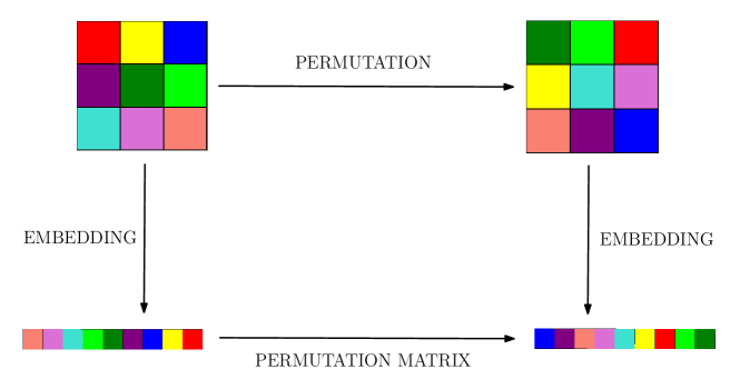
Figure 10: Diagram identifying two signals permutation apart from each other on a $3\times 3$ grid, where each color represents the signals’ value at the pixels. Notice the diagram to commute.

Several important properties of permutation matrices are noteworthy to be recalled. For example, by construction, it is easy to see that if $\sigma$ is a permutation matrix, then it is an orthogonal transformation on $\mathbb{R}^{n}$. Besides, if $\sigma$ and $\sigma^{\prime}$ are two permutations on the grid, then the composition $\sigma\circ\sigma^{\prime}$ also is a permutation, whose associated permutation matrix is given by the product $\sigma\cdot\sigma^{\prime}$. Consequently, if $\Sigma$ is a group of grid permutations, we may define an orthogonal representation by considering its permutation matrices. This shows that every group of permutations is a subgroup of $\mathrm{O}(n)$. We might be interested to determine whether these also are contained in smaller Lie groups, something that is achieved for the special cases below.

Given a permutation group $\Sigma$ and an initial signal $f$, its orbit $\{\sigma\cdot f^{\uparrow}\mid\sigma\in\Sigma\}$ is a subset of $\mathbb{R}^{n}$, and is included in the orbit of a representation of a compact Lie group. An instructive case is that of a cyclic group $G$, say of order $p$, generated by a permutation $\sigma$. Supposing that the permutation is even, the corresponding matrix is special orthogonal, hence can be written as $\exp(2\pi L/p)$ for a certain skew-symmetric matrix $L$. We see that the orbit takes the form

$$\big{\{}\exp(2\pi mL/p)\cdot f^{\uparrow}\mid m\in[0\dots p-1]\big{\}}.$$

In particular, it is a subset of the orbit of $f^{\uparrow}$ under the representation of $\mathrm{SO}(2)$ in $\mathbb{R}^{n}$ given by $\theta\mapsto\exp(2\pi\theta L)$. The lemma below shows that this observation holds for any Abelian group $\Sigma$, and that, in addition, the orbit can be projected in lower-dimensional subspaces, provided that they are chosen in accordance with the covariance matrix of the orbit.

Lemma 6.1.

Consider point cloud $X=\{x_{i}\}_{i=1}^{N}$ of $\mathbb{R}^{n}$ generated by the application of an Abelian permutation group $\Sigma$ of rank $d$ to an initial image, and which has been centered, i.e., $\sum_{i=1}^{N}x_{i}=0$. Then $X$ lies on an orbit of a representation of the torus $T^{d}$. More precisely, there exists a representation $\phi\colon T^{d}\rightarrow\mathrm{SO}(n)$, a point $x\in\mathbb{R}^{n}$, and $p_{1},\dots,p_{d}\in\mathbb{Z}^{d}$ such that

$$X=\big{\{}\phi\big{(}2\pi m_{1}/p_{1},\dots,2\pi m_{d}/p_{d}\big{)}\cdot x\mid m_{1}\in[0\dots p_{1}-1],~{}\dots,~{}m_{d}\in[0\dots p_{d}-1]\big{\}}.$$

Moreover, suppose the point cloud is projected into a subspace that is a sum of eigenspaces the data’s covariance matrix, all of which have even dimensions. Then it lies on an orbit of $T^{d}$.

Proof.

We first suppose that $\Sigma$ has rank one, that is to say, is generated by a permutation matrix $\sigma$, and denote its order as $p$. If $x$ is any point of $X$, we can write

$$X=\big{\{}\sigma^{m}x\mid m\in[0\dots p-1]\big{\}}.$$

We distinguish two cases. If $\sigma$ is an even permutation, then it has matrix determinant $1$. That is, it belongs to $\mathrm{SO}(n)$, hence there exists a skew-symmetric matrix $L$ such that $\sigma=\exp(2\pi L/p)$. The powers of $\sigma$ takes the form $\exp(2\pi mL/p)$ for $m\in[0\dots p-1]$, and we deduce that $X$ is included in the orbit of $x$ under the representation $\theta\mapsto\exp(2\pi\theta L/p)$ of $\mathrm{SO}(2)$.

On the other hand, if $\sigma$ is an odd permutation, then it does not admit a real logarithm. In this case, we remember that $\sigma$ has eigenvalues $1$ and $-1$. The first comes from the fact that the vector $w=(1,\dots,1)\in\mathbb{R}^{n}$ is stabilized by $\sigma$, and the second is obtained from the decomposition of $\sigma$ into disjoint cycles. Let $w^{\prime}$ denote an eigenvector associated to $-1$. We have an orthogonal decomposition $\mathbb{R}^{n}=V\oplus\langle w\rangle\oplus\langle w^{\prime}\rangle$. The matrix $\sigma$ stabilizes $V$. Consequently, in this decomposition of $\mathbb{R}^{n}$, it can be written

$$\sigma=\mathrm{diag}\big{(}O^{\prime},1,-1\big{)}$$

for a certain $O^{\prime}\in\mathrm{O}(n-1)$. The submatrix $\mathrm{diag}(1,-1)$ has determinant $-1$, hence that of $O^{\prime}$ is $1$, meaning that it admits a real logarithm: $O^{\prime}=\exp(2\pi L/p)$. Besides, we note that the action of $\sigma$ on $X$ is the same as that of

$$\sigma^{\prime}=\mathrm{diag}\big{(}O^{\prime},-1,-1\big{)}.$$

Indeed, the data has been centered, hence the point $x$ is orthogonal to the penultimate axis $\langle w\rangle$. Moreover, $\sigma^{\prime}$ is now a matrix of determinant $1$, reducing to the first case.

More generally, let us suppose that $\Sigma$ has rank $d$, generated by a set of permutations $\{\sigma_{1},\dots,\sigma_{d}\}$ of order $p_{1},\dots,p_{d}$. As we have seen above, each $\sigma_{i}$ can be written as $\exp(2\pi L_{i}/p_{i})$ for a certain skew-symmetric matrix $L_{i}$. Moreover, since the matrices $\sigma_{i}$’s commute by assumption, we can choose the $L_{i}$’s to commute. We conclude that $X$ is included in the orbit of $x$ under the well-defined representation of $T^{d}$:

$$(\theta_{1},\dots,\theta_{d})\longmapsto\prod_{j=1}^{d}\exp(2\pi\theta_{j}L_{j}/p_{j}).$$

Next, we prove the second part of the lemma, starting with the case $d=1$, and supposing, without loss of generality, that $n$ is even. The point cloud $X$ can be written as $\{\phi(2\pi m/p)\cdot x\mid m\in[0\dots p-1]\}$ for some representation $\phi$ of $\mathrm{SO}(2)$. By decomposition into irreps, there exists $\omega\in\mathbb{Z}^{n/2}$ and basis of $\mathbb{R}^{n}$ where $\phi$ is equal to

$$\theta\longmapsto\mathrm{diag}\big{(}R(\omega_{1}),\dots,R(\omega_{n/2})\big{)}.$$

and where $R$ is the $2\times 2$ rotation matrix defined in Example 2.2. Moreover, using the explicit expression given in Lemma A.1 (in Appendix A.2.4), the covariance matrix of $X$ takes the form

$$\frac{1}{2}\begin{pmatrix}x_{1}^{2}+x_{2}^{2}&&&&&\\ &x_{1}^{2}+x_{2}^{2}&&&&\\ &&\ddots&&&\\ &&&&x_{n-1}^{2}+x_{n}^{2}&\\ &&&&&x_{n-1}^{2}+x_{n}^{2}\end{pmatrix}.$$

In particular, if $\lambda$ is any eigenvalue, then the eigenspace associated with $\lambda$ is a sum of stable planes of the representation. We deduce the statement of the lemma. More generally, the result still holds if $\Sigma$ has rank $d$, because the covariance matrix can still be written as a diagonal matrix, with repeated eigenvalues on the stable planes. ∎

Example 6.2 (Gorillas on circle).

Consider a dataset formed of 65 3-channel gorilla images with $120\times 130$ pixels each. As illustrated by the left-side of Figure 11, these images are formed by subsequent applications of the translation group $\Sigma=\langle(0,2)\rangle\simeq\mathbb{Z}/65\mathbb{Z}$ to any initial image, meaning that the respective embeddings lie exactly on an orbit of this $\Sigma$ in $\mathbb{R}^{120\times 130\times 3}$. Alternatively, by Lemma 6.1, these embeddings must also be samples of an orbit of $T^{1}=\mathrm{SO}(2)$ on this space, whose specific representation type can be given by LieDetect. The middle image of Figure 11 indicates the bottom eigenvalues of Step 2’s $\Lambda$ when applied to the embedded gorilla images, with dimension reduced to 6 through PCA. With only one eigenvalue particularly small, it is noteworthy that the result of Lemma 6.1 in this particular case may be directly observed through the application of LieDetect’s Step 2. The estimated representation type for this problem was of weights $(1,2,3)$. Good convergence of Algorithm 3.1 in this case can be confirmed by the right-most image of Figure 11, where the reconstructed orbit (magenta) is visually identified very close to the embedded figures (black)—in fact, the estimated Hausdorff distance was of only $0.0071$.

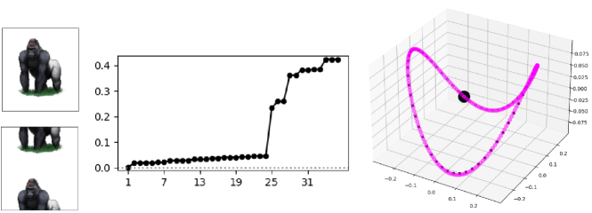
Figure 11: Left: sample of the data set of gorilla images translated in a $\mathrm{SO}(2)$-like permutation group. Middle: bottom eigenvalues of the Lie-PCA operator $\Lambda$, where one solution is clearly distinguishable. Right: estimated orbit (magenta) for the orbit of the embedded figures in dimension 6, and reduced, through PCA, to dimension 3 for visualization purposes.

Example 6.3 (Gorillas on torus).

Let us generalize the prior example to higher dimensions. In [84], the author used Rips filtrations, together with the newly introduced Stiefel-Whitney filtrations, in a data set of gorilla images, now translated horizontally and vertically (Figure 12) to identify the embedded point cloud of 3900 images of size $130\times 120$ as lying on the surface of a torus $T^{2}$, where each of the points corresponds to a translation on the group $\mathbb{Z}/60\mathbb{Z}\times\mathbb{Z}/65\mathbb{Z}$ applied to some of the gorilla images.

We can, however, consider this torus as the representation of the group itself on the embedding space through an injection map and, as such, inquire about the representation’s weights. Using again a 3-channel framework, we reduce the data’s dimension to 6 by PCA and apply LieDetect to the output. The rightmost plot of Figure 12 shows the result of Step 2, where a solution space of dimension 2 can be clearly identified. Using that the skew-symmetrized outputs of Step 2 commute up to $10^{-13}$ in matrix Frobenius norm, we apply the normal matrices solution to torus data, giving the representation type of $(1,1,2)$ and $(1,37,38)$. The Hausdorff distance was only $0.015$, which consider small.

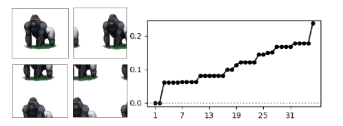
Figure 12: Left: sample of the data set of gorilla images translated in a $T^{2}$-like permutation group. Right: bottom eigenvalues of the matrix $\Sigma$, where two values are clearly distinguishable.

6.2 Harmonic analysis

Below, we suggest an application, in the context of regression with abstract harmonic analysis, of the knowledge of the data set to be close to representation orbit. Although this example could be fully derived from the harmonic analysis of finite Abelian groups, without mentioning Lie theory at all, if we were given only the data set as a point cloud in $\mathbb{R}^{120\times 130\times 3}$, it would require a lot of creativity to realize that it corresponds to pixel permutations of the same image, whereas the fact that they lie on the surface of an orbit of a $T^{2}$ representation is achievable by simply applying LieDetect.

Example 6.4 (Regression via harmonic analysis).

Let us refer back to the gorillas on torus data set $\{f_{i}\}_{i=1}^{N}$ of Example 6.3, observed to correspond to a torus representation orbit (see Figure 12). Because of its equivalence with the torus $T^{2}$, any function $F\colon\{f_{i}\}_{i=1}^{N}\rightarrow\mathbb{C}$ with domain the set of images may be seen as the restriction $\widetilde{F}|_{\{f_{i}\}_{i=1}^{N}}$ of a map $\widetilde{F}:T^{2}\to\mathbb{C}$, which is enough well-behaved so to be expressed as

$$\widetilde{F}(\theta_{1},\theta_{2})=\sum_{n_{1},n_{2}\in\mathbb{Z}}\widehat{f}(n_{1},n_{2})\exp(2\pi i\theta_{1}n_{1})\cdot\exp(2\pi i\theta_{2}n_{2})$$

for the usual coordination $(\theta_{1},\theta_{2})$ of $T^{2}$ and the Fourier coefficients $\widehat{f}$, as defined in Example 2.8. In particular, let us consider the map $F$ that indicates the gorilla’s head center position $(x,y)$, for $(x,y)$ in the permutation group $\mathbb{Z}/{120}\mathbb{Z}\times\mathbb{Z}/{130}\mathbb{Z}$. We may calculate it as

$$\widetilde{F}(\theta_{1},\theta_{2})=\sum_{n_{x},n_{y}\in\mathbb{Z}}\widehat{f}(n_{x},n_{y})\exp(2\pi i\theta_{1}n_{x}/N_{x})\cdot\exp(2\pi i\theta_{2}n_{y}/N_{y}),$$

where $N_{x}$ and $N_{y}$ are, respectively, the orders of the generators of translation in the horizontal and vertical directions (here $N_{x}=60$ and $N_{y}=65$). Notice that, because $\widehat{f}(n_{x},n_{y})$ are just coefficients, they may be learned through linear regression. For instance, in [64], the authors give a Maximum Likelihood Estimation (MLE) of the regression vector $\beta$ for complex coefficients as

$$\widehat{{\beta}}=(A^{\dagger}A)^{-1}A^{\dagger}\vec{F}(i,j),$$

where the dagger represents the complex conjugate, $\vec{F}(x,y)$ is the set of all outputs of $F$, and $A$ is the regressor matrix that, for a fixed pair $(x,y)$, takes here the form

$$A(x,y)=\begin{pmatrix}\exp\big{(}2\pi i\big{(}-\nu_{\mathrm{max}}\frac{x}{N_{x}}-\nu_{\mathrm{max}}\frac{y}{N_{y}}\big{)}\big{)}\\ \exp\big{(}2\pi i\big{(}-\nu_{\mathrm{max}}\frac{x}{N_{x}}-(\nu_{\mathrm{max}}+1)\frac{y}{N_{y}}\big{)}\big{)}\\ \vdots\\ \exp\big{(}2\pi i\big{(}(-\nu_{\mathrm{max}}+1)\frac{x}{N_{x}}-\nu_{\mathrm{max}}\frac{y}{N_{y}}\big{)}\big{)}\\ \vdots\\ \exp\big{(}2\pi i\big{(}\nu_{\mathrm{max}}\frac{x}{N_{x}}+\nu_{\mathrm{max}}\frac{y}{N_{y}}\big{)}\big{)}\\ \end{pmatrix}^{\top}.$$

Notice that $\nu_{\mathrm{max}}$, the maximal frequency, is a natural number hyperparameter which, the bigger it becomes, the finer an approximation of $F$ we achieve. Of course, the best result happens only at the limit of infinite; nevertheless, because the series is known to converge for every input, for most functions, taking values of $\nu_{\mathrm{max}}$ of order $10$ is often enough. We will call, from now on, this whole framework of estimating $F$ through the harmonic decomposition of the torus a ‘harmonic analysis model’.

Figure 13 illustrates this regression problem: we consider the Gaussian $130\times 120$ pixels filter, displayed at the first column and convolute it with each of the images, therefore creating the map $F:\{f_{i}\}_{i=1}^{N}\to\mathbb{R}$. The second column shows the result of component-wise multiplying this filter with one of the images, that is, the sub-operation of convolution before summing the elements. From it, we see that convolution erases the area outside the white region of the filter, meaning that because the gorilla is of darker shades than the background, the more of it that lies in the blank region, the larger $F$ becomes. The third column of Figure 13 is a color map of $F$ for each of the images, where the coordinates $(x,y)$ are used to represent the gorilla with head at $(2x,2y)$. Finally, the last column shows the reconstruction of the function $F$ through harmonic analysis, where the full data set was used and $\nu_{\mathrm{max}}$ was set to $10$. The almost perfect agreement of these last two plots suggests good convergence of the model, even for such a ‘small’ number of parameters.

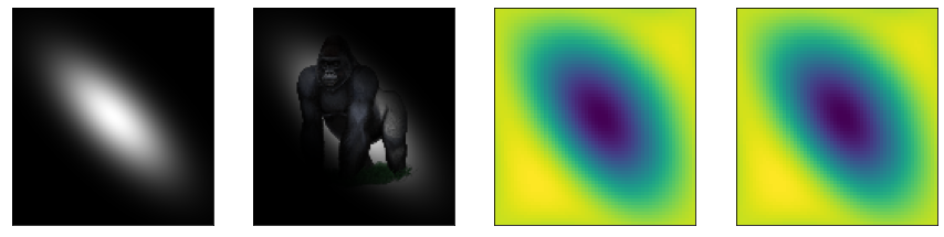
Figure 13: First: Gaussian filter to be convoluted with images. Second: component-wise product of Gaussian filter and centralized gorilla image. Third: color plot indicating the map $F$ of the gorilla translated to a point $(x,y)$ and the Gaussian filter. Fourth: reconstruction of the map $F$ reconstruction through the harmonic analysis model, as indicated in the text.

Nonetheless, in making the rightmost plot of Figure 13, the full data set available was used, something unfitting for an actual regression problem. Therefore, to access the harmonic analysis model’s predictive power, we separated the data, here seen as the images (inputs) and respective values of $F$ (output) into a training set of $90\%$ the original size, and a test set with the remaining $10\%$. Besides, to assess its performance, we compare its results to three other classical machine learning models. Figure 14 shows the predictions of the models, trained only with the train data set, to all the translated images, whereas Table 1 shows the observed mean squared error on test data. Although in both cases harmonic analysis is identified to perform better, we stress that this list of models is far from exhaustive and it is very likely that fine-tuning extra hyperparameters on the random forest and neural networks implementations would allow for models that suppress the Lie group oriented technique. Moreover, the embedded gorilla images have a close-to-zero deviation from the underlying torus manifold, which is very unlikely to happen in applications. The point, however, is that through the geometric knowledge of data, competitive solutions to machine learning tasks are possible, indicating that the methods described in this article represent not only gains in terms of explainability but also in terms of accuracy itself.

Model	MSE on test data
Harmonic analysis	0.02057
Random Forest	$0.09336$
Support Vector Machine	$24.91$
Neural Network	$25.33$

Table 1: Models trained on $90\%$ of the gorilla image data set (left column) and their test mean squared error (right column). The harmonic analysis model was estimated as described in the main text. The random forest used sklearn’s implementation default parameters. For the SVM, we used RBF kernel and grid search on the sets $\{0.1,1,10,100,1000\}$ and $\{0.1,0.2,0.5,1\}$ for the parameters $C$ and $\epsilon$, respectively. Finally, different neural network architectures with further $10\%$ data dedicated to validation were tested and the reported result corresponds to the prediction of the one which achieved smallest MSE on test data.

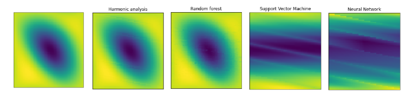
Figure 14: First figure left: color plot of the target function. Four figures right: color plots of estimated function by different models using $90\%$ of available data, as describe in Table

6.3 Hamiltonian systems

As mentioned in Example 1.3, Lie group actions also play an important role in physics, which can be exemplified in the study of Hamiltonian systems. These systems can here be understood as fully described, for all time $t\in\mathbb{R}$, by a position vector $\textbf{q}(t)\in\mathbb{R}$, an associated momenta vector $\textbf{p}(t)\in\mathbb{R}$, and a function $H$ called the Hamiltonian and often equal to the system’s total mechanical energy, such that the system’s evolution in time is dictated by Hamilton’s equations

$$\frac{\mathrm{d}\textbf{p}}{\mathrm{d}t}=-\frac{\partial H}{\partial\textbf{q}}~{}~{}~{}~{}~{}~{}~{}~{}~{}~{}~{}~{}~{}~{}\frac{\mathrm{d}\textbf{q}}{\mathrm{d}t}=\frac{\partial H}{\partial\textbf{p}}.$$

On other words, letting $\textbf{z}=(\textbf{q},\textbf{p})$,

$$\frac{\mathrm{d}\textbf{z}}{\mathrm{d}t}=\begin{pmatrix}0&I_{n}\\ -I_{n}&0\end{pmatrix}\textbf{z}=\omega\textbf{z},$$

where the tensor $\omega$ is the canonical symplectic form in $\mathbb{R}^{2n}$. In general, physical information about the systems is retrieved through observables, that is, real-valued smooth functions $f:\mathbb{R}^{2n}\to\mathbb{R}$. One may impose, through the introduction of Poisson brackets, an infinite dimensional Lie algebra structure in the set of observables by

$$\{f,g\}=-\mathrm{d}f^{\top}\cdot\omega\cdot\mathrm{d}g=\sum_{a=1}^{n}\frac{\partial f}{\partial q_{a}}\frac{\partial g}{\partial p_{a}}-\frac{\partial f}{\partial p_{a}}\frac{\partial g}{\partial q_{a}}.$$

Moreover, an observable is called conserved if its value does not change through time. Assuming the Hamiltonian to have no time dependence, a statement equivalent to the conservation of energy, we have that $f$ is conserved if and only if, in terms of Poisson bracket,

$$0=\frac{\mathrm{d}f}{\mathrm{d}t}=\{H,f\}.$$

Back to Lie groups, we see that a representation $L:G\to\mathrm{GL}_{2n}(\mathbb{R})$ on $\mathbb{R}^{2n}$ preserves the the system’s dynamics only if

$$L(g)^{*}\omega=\omega~{}~{}~{}~{}\forall g\in G,$$

in which case $L$ is said to be a symplectomorphism or canonical. If the group $G$ is compact, then the existence of a symplectic representation on $\mathbb{R}^{2n}$ implies a canonical map from the group’s Lie algebra $\mathfrak{g}$ to the set of observables under Poisson brackets, known as the comoment map [30, 91]. Moreover, an observable $f$ is conserved if and only if it is an image of some comoment map derived from a symplectic action of a Lie group $G$ in $\mathbb{R}^{2n}$. Although it is not true that only when the motion $\textbf{z}(t)$ lies on the orbit of a Lie group symplecitmorphism that there are conserved observables, the converse is true, that is, if we have as data a set of $\textbf{z}(t)$ that lies on a hypersurface of $H$, which also coincides with the orbit of a symplectomorphism, then there is a subalgebra of observables isomorphic to $\mathfrak{g}$. This suggests the usefulness of determining whether a point cloud sampled on a hypersurface of $H$ also lies on an orbit of an unknown Lie group, and of determining which group that is.

We will give here two examples of applications of LieDetect to data sets representing the state space of physical systems. The first is not directly related to the conservation of quantities, although it is the orbit of a $\mathrm{SO}(2)$ representation, allowing the construction of some missing configurations (i.e., orbit completion). The second transforms the usual angular momentum conservation into data, letting the comoment map formalism be used.

Example 6.5 (Multidimensional harmonic oscillator).

Consider a particle in $\mathbb{R}^{n}$, with $n$ sets of perpendicular springs attached to it, as visualized in Figure 15. By aligning the coordinate axes with the $n$ directions of the springs’ attachment, the system’s total energy, in the regime of Hooke’s law, becomes,

$$H=\sum_{i=1}^{n}\frac{p_{i}^{2}}{2m}+\frac{k_{i}q_{i}^{2}}{2},$$

where $m$ is the particle’s mass, here taken to be $m=1$, and $k_{i}$ are constants, related to each spring’s material and length. Applying Hamilton’s equation to this energy, we have

$$\begin{split}\dot{q_{i}}=p_{i}~{}~{}~{}~{}~{}~{}~{}~{}~{}~{}~{}~{}~{}~{}\dot{p}_{i}=-k_{i}q_{i},\end{split}$$

for which, assuming the particle is released from rest at some initial position $\mathbf{q}(0)$, solves for

$$q_{i}=q_{i}(0)\cos(\sqrt{k_{i}}t)~{}~{}~{}~{}~{}~{}~{}~{}~{}~{}~{}~{}~{}~{}p_{i}=-\sqrt{k_{i}}\sin(\sqrt{k_{i}}t).$$

The curve the system traces in phase space is an orbit of a $\mathrm{SO}(2)$ representation: letting

$$M=\text{diag}\bigg{(}\frac{1}{q_{1}^{2}(0)},\frac{1}{k_{1}},\dots,\frac{1}{q_{n}^{2}(0)},\frac{1}{k_{n}}\bigg{)},$$

we define the $\mathrm{SO}(2)$ representation in $\mathbb{R}^{n}$, following the notations of Example 2.3, as

$$\phi=M^{1/2}\big{(}\phi_{-\sqrt{k_{1}}}\oplus\dots\oplus\phi_{-\sqrt{k_{n}}}\big{)}M^{-1/2},$$

which is a representation of normalized weights $(\sqrt{k_{1}},\dots,\sqrt{k_{n}})$, provided the ratios between them can be always chosen to be integers, otherwise the system does not describe a $\mathrm{SO}(2)$-orbit.

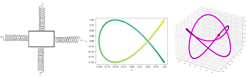
Figure 15: Left: diagram of a two-dimensional harmonic oscillator. Middle: positions of a full revolution on the $x$ (horizontal) and $y$ (vertical) coordinates of the harmonic oscillator with $k_{x}=4$ and $k_{y}=9$ released from rest at the point $x_{0}=y_{0}=1$. Right: 300 samples from the phase space curve (black) normalized via Step 1 to the unit sphere, together with the predicted orbit (magenta) computed with Algorithm 3.1.

Consequently, if readings of the particle’s position and momenta are available as a data set, we may apply Algorithm 3.1 not only to discover the ratio between the unknown constants $k_{i}$ but also to complete the orbit by generating points in the phase space that, although the system passes through, are not measured. Moreover, we recall that the related conserved quantity to this action corresponds to the energy $H$ itself, allowing us to derive such an important law of physics from data only. Figure 15 shows the application of LieDetect to data consisting of $N=300$ points simulated for a system with parameters

$$x_{0}=y_{0}=1,~{}~{}~{}~{}~{}k_{x}=9~{}~{}~{}~{}~{}\mathrm{and}~{}~{}~{}~{}~{}k_{y}=4,$$

and for the time $t$ equally spaced on the interval $[0,3\cdot 2\pi]$. The underlying representation has weights $(\sqrt{k_{x}},\sqrt{k_{y}})=(3,2)$. We start noticing that, unless all the parameters are equal, the orbit does not already lie on a sphere of $\mathbb{R}^{4}$, making Step 1 necessary. On the other hand, as the orbit spans the ambient space, no prior dimension reduction with PCA is required. As the graphs of Figure 15 suggest, the algorithm seems to converge well to the expected orbit. This fact is confirmed by the table below, showing the costs obtained by the minimization program in Step 3 as a function of the weights, exhibiting $(2,3)$ as the optimal representation.

Weights	$(1,1)$	$(1,2)$	$(1,3)$	$(2,3)$
Costs	$0.077$	$0.031$	$0.139$	$1.059\times 10^{-9}$

Example 6.6 (Conservation of angular momentum).

Consider the symplectic action of $\mathrm{SO}(3)$ on the cotangent bundle $\mathrm{T}^{*}\mathcal{M}\simeq\mathbb{R}^{6}$ of $\mathcal{M}=\mathbb{R}^{3}$ given by $O\cdot(\textbf{q},\textbf{p})=(O\cdot\textbf{q},O\cdot\textbf{p})$, and suppose $H$ is a system’s energy which is conserved by this action, meaning that $U(\textbf{q})$ may only depend on radial coordinates. These systems are called central forces and examples range from the interaction between point charges to Kepler’s planetary motion. A well-known fact from Hamiltonian mechanics [91] is that there exists a comoment map $P$, taking the usual basis elements $X_{i}$ from $\mathfrak{so}(3)$ (Example 2.1) to observables $\mathbb{R}^{6}\rightarrow\mathbb{R}$, and which is given by

$$P(L_{i})=(\mathbf{p}\times\mathbf{q})_{i}=\mathbf{l}_{i},$$

where $i\in\{1,2,3\}$, meaning that the quantity $\mathbf{l}$, known by physicists as angular momentum, is conserved for central forces problems. Moreover, only scalar multiples of the angular momentum vectors are possible images of the comoment map $P$, for this particular representation of $\mathrm{SO}(3)$.

LieDetect can be used to identify this conservation of angular momentum from data. For example, suppose we gathered as lab data an orbit of this representation (of course, without previous knowledge that it is an orbit of a representation), which can be achieved, for example, by recording the states of classical electrons in different hydrogen atoms. Here, we have 1000 points sampled uniformly on the orbits of radii 1 on the split three-dimensional subspaces, after an application of some random orthogonal change of coordinates. Although this data lies on an orbit of a $\mathrm{SO}(3)$-representation of weights $(1,1)$, straight applying LieDetect, without PCA, to the whole phase space data would yield incorrect results (left side of Figure 16). This is because there would be a subspace fully perpendicular to the orbit, forcing the Lie-PCA operator $\Lambda$ to have many more small eigenvalues than it should. This issue can be solved in two steps: first, we apply PCA to reduce the data’s dimension to 3 and confirm that this is, in fact, a representation of $\mathrm{SO}(3)$ (center of Figure 16); then, we split the original full set in $\mathbb{R}^{6}$ into position and coordinates, apply LieDetect to each subset, and therefore show that the representations are of the same weights, with the full orthogonal change of coordinates given by the block sum of the identified matrices (right side of Figure 16). Because we derive the representation to be of weights $(1,1)$, we have by the above arguments that the scalar multiples of the angular momentum vector must be conserved in this type of system.

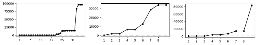
Figure 16: Eigenvalues of Lie-PCA $\Lambda$ for the full data set (left), for the data set with dimension reduced to 3 through PCA (center), and for the projection onto position coordinates (right).

7 Conclusion

We presented in Algorithm 3.1 what we believe to be the first method in literature to identify, in an unsupervised fashion, Lie group representation orbits in point clouds. Moreover, because we estimate the equivalence class of the representation in the process, the algorithm can be used to reconstruct the orbit, eventually allowing to determine which compact Lie groups generate the orbit. There are several constraints assumed in the application of the algorithm, that we have made explicit in Theorem 5.21, and which we aim to sequentially loose in future works.

The first line of expansion consists in lifting the representation constraint. This does not only mean expanding Algorithm 3.1 to non-linear actions on point clouds, although it definitely is a direction to further explore, but also consists in considering more inventive maps from Lie groups. For example, there is in Physics literature a genuine interest on projective representations, which are maps $\phi:G\to\mathrm{GL}(m,\mathbb{C})/\mathbb{C}^{*}I$, where $\mathbb{C}^{*}I$ is the set of nonzero multiples of the identity. These non-traditional representations are the most well-known objects used in the traditional theory of classification of $\mathrm{Spin}(n)$ complex representations, giving rise to the definition of the geometric objects known as ‘spinors’ . Similar derivations of spinors can be achieved by means of Clifford algebras, as briefly introduced in [9]. Besides, infinite dimensional representations, due to their natural translation to vector field theory and their important role in quantum mechanics, are also worth exploring.

Expanding the methods to more general groups also deserves to be investigated. Starting with finite groups, these have already received a fair share of literary interest in machine learning. Many, if not all, of the properties used in deriving Algorithm 3.1, such as orthogonality of general representations and classification of the irreducible ones, also work for this class of groups. For more general Lie groups, though, many of the properties here assumed fail to hold. In fact, although some of the non-compact cases such as Poincaré and Lorentz’s groups have their representations well-studied for decades, this does not mean that they are easy to work with. For both of these cases, for example, no non-trivial finite-dimensional representation is unitary [91], which deeply impact our computations. On the other hand, given a general manifold $\mathcal{M}$ embedded in some $\mathbb{R}^{n}$, the description of its symmetry group, $\mathrm{Sym}(\mathcal{M})$, may easily skip the compact boundary, justifying the interest in these less-well-behaved scenarios.

Finally, the methods here explored seem to present a fruitful field of applications to machine learning. As reviewed in Section 1, all existing architectures, including equivariant neural networks, do not require precise knowledge of representation types nor, sometimes, of the acting Lie group to properly work. We believe, on the other hand, that this important knowledge, which can be attained through Algorithm 3.1, may be used to suggest different inference architectures, which have the potential to overcome many of the challenges faced by current Lie group-aware techniques. Notice that these challenges do not necessarily restrict themselves to improvements in prediction capacity: in the many distinct areas discussed here, where Lie groups play a significant role—i.e., image processing, harmonic analysis, and classical mechanics—the existing techniques have already shown significant success, and the extra knowledge of the representation will probably signify better accuracy. Yet, there are many fields, such as particle physics, where the knowledge of the precise representation type becomes crucial, and machine learning algorithms that incorporate the precise representation equivalence class in their architecture may prove to be the correct form of addressing the inference tasks.

Acknowledgements.

The original work behind this paper was developed for HE’s master’s thesis, supervised by RT. We are mostly in debt to César Camacho, who was HE’s co-advisor, as well as the members of the thesis jury, Clément Maria, Eduardo Mendes, and Jameson Cahill, not only for agreeing in evaluating the original work but also for many valuable inputs.

Appendix A Additional comments

A.1 Notations

Notation conventions are summarized in the table below.

Symbol	Meaning
$\langle v_{1},\dots,v_{N}\rangle$	Vector subspace spanned by the vectors $v_{1},\dots,v_{N}\in\mathbb{R}^{n}$
$[i\dots j]$	The set of integers between $i$ and $j$ included
$X$	A finite subset of $\mathbb{R}^{n}$
$\mathrm{diag}(A_{1},\dots,A_{n})$	Block-diagonal matrix whose blocks are the matrices $A_{1},\dots,A_{n}$
$\langle A,B\rangle_{\mathrm{F}}$ or $\langle A,B\rangle$,	Frobenius inner product and Frobenius norm of matrices $A,B\in\mathrm{M}_{n}(\mathbb{R})$
$\|A\|_{\mathrm{F}}$ or $\|A\|$	(also known as the $L^{2}$-norm or Euclidean norm)
$\|A\|_{\mathrm{op}}$	Operator norm of a matrix $A\in\mathrm{M}_{n}(\mathbb{R})$
$\Pi\big{[}V\big{]}$ or $\Pi_{V}$	Orthogonal projection matrix on a subspace $V\subset\mathbb{R}^{n}$ or $V\subset\mathfrak{so}(n)$
$\mathrm{Isom}(\mathcal{M})$,	Isometry (resp. symmetry) group of a Riemannian manifold $\mathcal{M}$
$\mathrm{Sym}(\mathcal{M})$	isometrically embedded in $\mathbb{R}^{n}$ (see Section 2.1.4)
$\mathrm{T}_{x}\mathcal{M}$, $\mathrm{N}_{x}\mathcal{M}$	The tangent (resp. normal) space of a submanifold $\mathcal{M}\subset\mathbb{R}^{n}$ at $x\in\mathcal{M}$
$G$, $\mathfrak{g}$, $\phi$, $\mathcal{O}$	A Lie group, a Lie algebra, a representation, an orbit of representation
$\widehat{\mathfrak{h}}$, $\widehat{\phi}$, $\widehat{\mathcal{O}}_{x}$, $\mu_{\widehat{\mathcal{O}}}$	Outputs of Algorithm 3.1 (defined in Section 3.5)
$\text{Rep}(G,\mathbb{R}^{n})$,	The equivalence classes (resp. orbit-equivalence classes) of almost-
$\text{OrbRep}(G,\mathbb{R}^{n})$	faithful representations of the Lie group $G$ in $\mathbb{R}^{n}$ (see Section 2.2.3)
$\text{Irr}(G)$	A set consisting of a choice of an orthogonal representative
	for each equivalence class of irreps of the Lie group $G$
$\mathfrak{orb}(G,n)$	Pushforward algebras $\big{\{}\big{(}B^{\phi_{1}},\dots,B^{\phi_{p}}\big{)}\mid(\phi_{1},\dots,\phi_{p})\in\mathrm{OrbRep}(G,n)\big{\}}$
	for an arbitrary choice of orthogonal representatives (see Section 2.3.2)
$\mathcal{G}^{\mathrm{Lie}}(d,\mathfrak{so}(n))$,	The Grassmannian (resp. Stiefel) variety of $d$-dimensional
$\mathcal{V}^{\mathrm{Lie}}(d,\mathfrak{so}(n))$	Lie subalgebras of $\mathfrak{so}(n)$ (see Section 2.3.1)
$\mathcal{G}(G,\mathfrak{so}(n))$,	The Grassmannian (resp. Stiefel) variety of $d$-dimensional
$\mathcal{V}(G,\mathfrak{so}(n))$	Lie subalgebras of $\mathfrak{so}(n)$ pushforward from $G$ (see Section 2.3.2)
$\Lambda$	Lie-PCA operator (defined in Equation (8))
$\Lambda_{\mathcal{O}}$	Ideal Lie-PCA operator (defined in Equation (30))
$\mathrm{d}_{\mathrm{H}}\big{(}X|Y\big{)}$	Non-symmetric Hausdorff distance (resp. Hausdorff distance)
$\mathrm{d}_{\mathrm{H}}(X,Y)$	between two compact subsets $X,Y\subset\mathbb{R}^{n}$ (see Section 3.5.1)
$\mathrm{W}_{p}(\mu,\nu)$	Wasserstein distance between $p$-integrable measures (see Section 3.5.2.)
$\mu_{X}$, $\mu_{G}$, $\mu_{\mathcal{O}}$	Empirical measure on a point cloud $X$, Haar measure on
	a compact Lie group $G$, uniform measure on an orbit $\mathcal{O}$
$\Sigma[\mu]$	Covariance matrix of the measure $\mu$ (defined in Equation (23))
$\Gamma(G,n)$	Rigidity of the derived representations of $G$ in $\mathbb{R}^{n}$ (resp. with
$\Gamma(G,n,\omega_{\max})$	weights at most $\omega_{\max}$) (defined in Equation (47))

A.2 Supplementary results

A.2.1  Isometry and symmetry groups

Proof of Equation (2).

As it is the case for any Lie subgroup of $\mathrm{GL}_{n}(\mathbb{R})$, we have the equality

$$\mathfrak{sym}(\mathcal{M})=\big{\{}A\in\mathrm{M}_{n}(\mathbb{R})\mid\forall t\in\mathbb{R},~{}\exp(tA)\in\mathrm{Sym}(\mathcal{M})\big{\}}.$$ (54)

It can be found for instance in [77, Th. 4.1]. Let us first show that the set defined in Equation (54) is equal to that of Equation (2). If $A$ is a matrix such that $\exp(tA)\in\mathrm{Sym}(\mathcal{M})$ for all $t\in\mathbb{R}$, then for any $x\in\mathcal{M}$ the curve $t\mapsto\exp(tA)x$ lies in $\mathcal{M}$, hence its derivative at $0$, equal to $Ax$, lies in $\mathrm{T}_{x}\mathcal{M}$. Conversely, suppose that $A$ satisfies $Ax\in\mathrm{T}_{x}\mathcal{M}$ for all $x\in\mathcal{M}$. Then for any $x_{0}\in\mathcal{M}$, the curve $\gamma\colon t\mapsto\exp(tA)x_{0}$ has derivative $\gamma^{\prime}(t)=A\gamma(t)$, hence $\gamma^{\prime}(t)\in\mathrm{T}_{\gamma(t)}\mathcal{M}$, provided that $\gamma(t)\in\mathcal{M}$. Consequently, the curve $\gamma$ satisfies an ordinary partial differential equation on the submanifold $\mathcal{M}$, showing that $\gamma(t)$ lies in $\mathcal{M}$. ∎

A.2.2  Irreps of $\mathfrak{su}(2)$

As mentioned in Example 2.7, using the double covering $\mathrm{SU}(2)\rightarrow\mathrm{SO}(3)$, any representation $\mathrm{SO}(3)$ yields a representation of $\mathrm{SU}(2)$, although the converse is not true. This may be expressed by parametrizing the complex irreducible representations of $\mathrm{SU}(2)$ through $m\in\mathbb{Z}^{+}$ (i.e., $\widehat{\mathrm{SU}}(2)=\mathbb{Z}^{+}$) or, following Physics literature, by $j=m/2\in\frac{1}{2}\mathbb{N}^{+}$. Then it is well known that while the representations with integer $j$ may be derived from (complex) representations of $\mathrm{SO}(3)$, the ones for half-integer $j$ may only be derived from the double cover $\mathrm{SU}(2)$ [91]. Moreover, the ones for integer $j$ are said to be of the real type, whereas the others are of quaternionic type [51]. Although all representations $\phi_{j}$ of real type may be transformed in real representations of $\mathfrak{su}(2)$ by a simple change of coordinates, defining representations in $\mathbb{R}^{2j+1}$, for representations of quaternionic type, this is only achievable if $2j\equiv 1\>(\text{mod }4)$, in which case the representation dimension is of $4j+2$ [50]. Therefore, if $\mathbb{R}^{n}$ receives a real irreducible representation of $\mathrm{SU}(2)$, then either $n$ is odd, in which case the representation is also a representation of $\mathrm{SO}(3)$, or $n$ is a multiple of 4. Moreover, for each choice of $n$, at most one representation of these groups can exist up to equivalence.

In [16], Campoamor-Stursberg derives the matrix elements of the real irreducible representations of $\mathrm{SO}(3)$ and $\mathrm{SU}(2)$. For the usual basis of $\mathfrak{so}(3)$, the commutators are given by

$$[L_{i},L_{j}]=\epsilon_{ijk}L_{k}$$

for the Levi-Civita symbol $\epsilon_{ijk}$. Denoting the weights as $j\in\frac{1}{2}\mathbb{N}$, when $j$ is an integer, the corresponding representation of $\mathfrak{su}(2)$ is of dimension $2j+1$ and have standard basis

$$\begin{split}[\mathrm{d}\phi(L_{1})]_{k,l}&=\bigg{(}\frac{1+(-1)^{k-1}}{2}\bigg{)}\bigg{(}\delta^{l}_{k+3}a_{\big{\lfloor}\frac{k+1}{2}\big{\rfloor}}+\delta^{l+1}_{k}a_{\big{\lfloor}\frac{k-1}{2}\big{\rfloor}}\bigg{)}\\ &\;\;\;-\bigg{(}a_{j}+\sqrt{\frac{j^{2}+j}{2}}\bigg{)}(\delta^{l}_{2j+1}\delta_{k}^{2j}-\delta^{l}_{2j}\delta^{2j+1}_{k})\\ &\;\;\;-\bigg{(}\frac{1+(-1)^{k}}{2}\bigg{)}\bigg{(}\delta^{l}_{k+1}a_{\big{\lfloor}\frac{k}{2}\big{\rfloor}}+\delta^{l+3}_{k}a_{\big{\lfloor}\frac{k-2}{2}\big{\rfloor}}\bigg{)}\\ [\mathrm{d}\phi(L_{2})]_{k,l}&=\delta^{l}_{k+2}a_{\big{\lfloor}\frac{k+1}{2}\big{\rfloor}}-\delta_{k}^{l+2}a_{\big{\lfloor}\frac{k-1}{2}\big{\rfloor}}\\ &\;\;\;-\bigg{(}a_{j}+\sqrt{\frac{j^{2}+j}{2}}\bigg{)}(\delta^{l}_{2j_{1}}\delta^{2j-1}_{k}-\delta^{l}_{2j-1}\delta_{k}^{2j+1})\\ [\mathrm{d}\phi(L_{3})]_{k,l}&=\frac{1}{4}\times[1+(-1)^{k}]\delta^{l+1}_{k}(2j+2-k)\\ &\;\;\;+[(-1)^{k}-1]\delta^{k+1}_{l}(2j+1-k),\\ \mathrm{where}~{}~{}~{}~{}~{}~{}~{}~{}~{}~{}~{}~{}~{}~{}~{}~{}~{}a_{l}&=\sqrt{\frac{2lj-l(l-1)}{4}},1\leq l\leq j,~{}~{}~{}~{}~{}~{}~{}~{}~{}~{}~{}~{}~{}~{}~{}~{}~{}~{}~{}~{}~{}~{}~{}~{}~{}~{}~{}~{}~{}~{}~{}\end{split}$$

and $\lfloor r\rfloor$ is the usual floor function. For half-integer $j$ such that $2j\equiv 1\pmod{4}$, the representation has dimension $4j+2$ and has standard basis

$$\begin{split}[\mathrm{d}\phi_{j}(L_{1})]_{k,l}&=\bigg{(}\frac{1+(-1)^{k-1}}{2}\bigg{)}\bigg{(}\delta^{l}_{k+3}a_{\big{\lfloor}\frac{k+1}{2}\big{\rfloor}}+\delta^{l+1}_{k}a_{\big{\lfloor}\frac{k-1}{2}\big{\rfloor}}\bigg{)}\\ &\;\;\;-\bigg{(}\frac{1+(-1)^{k-1}}{2}\bigg{)}(\delta^{l}_{k+1}a_{\big{\lfloor}\frac{k}{2}\big{\rfloor}}+\delta^{l+3}_{k}a_{\big{\lfloor}\frac{k-2}{2}\big{\rfloor}})\\ [\mathrm{d}\phi(L_{2})]_{k,l}&=\delta^{l}_{k+2}a_{\big{\lfloor}\frac{k+1}{2}\big{\rfloor}}-\delta_{k}^{l+2}a_{\big{\lfloor}\frac{k-1}{2}\big{\rfloor}}\\ [\mathrm{d}\phi(L_{3})]_{k,l}&=\frac{1}{4}\times[1+(-1)^{k}]\delta^{l+1}_{k}(2j+2-k)+[(-1)^{k}-1]\delta^{k+1}_{l}(2j+1-k).\end{split}$$

For other values of $j$, no real irreducible representations of $\mathfrak{su}(2)$ are possible.

A.2.3  Computations for Remark 5.10

Consider the representation $\phi\colon\mathrm{SO}(2)\rightarrow\mathrm{GL}_{4}(\mathbb{R})$ with distinct positive weights $(\omega_{1},\omega_{2})$, a real number $\epsilon>0$, $x_{0}=(1,0,\epsilon,0)\in\mathbb{R}^{4}$, and its orbit

$$\mathcal{O}=\big{\{}\big{(}\cos(\omega_{1}\theta),\sin(\omega_{1}\theta),\epsilon\cos(\omega_{2}\theta),\epsilon\sin(\omega_{2}\theta)\big{)}\mid\theta\in\mathrm{SO}(2)\big{\}}.$$

The tangent vector at $x_{0}$ is equal to $(0,\omega_{1},0,\epsilon\omega_{2})$. We then deduce from a computation that $(S_{x_{0}}\mathcal{O})^{\bot}$ admits $(B_{1},B_{2},B_{3})$ as an orthonormal basis, where

$$B_{1}=\begin{pmatrix}1&0&\epsilon&0\\ 0&0&0&0\\ 0&0&0&0\\ 0&0&0&0\end{pmatrix},~{}~{}~{}~{}~{}B_{2}=\begin{pmatrix}0&0&0&0\\ 0&0&0&0\\ 1&0&\epsilon&0\\ 0&0&0&0\end{pmatrix},~{}~{}~{}~{}~{}B_{3}=\begin{pmatrix}0&0&0&0\\ \epsilon\omega_{2}&0&\epsilon^{2}\omega_{2}&0\\ 0&0&0&0\\ -\omega_{1}&0&-\epsilon\omega_{1}&0\end{pmatrix}.$$

Besides, the representation $\phi$ on $\mathbb{R}^{4}$ induces a representation on $\mathrm{M}_{4}(\mathbb{R})$ by conjugation. Its restriction to $\mathfrak{so}(4)$ decomposes into irreps as $\mathfrak{so}(4)=\langle A_{1}\rangle\oplus\langle A_{2}\rangle\oplus\langle A_{3},A_{4}\rangle\oplus\langle A_{5},A_{6}\rangle$, where

$$A_{1}=\begin{pmatrix}0&-w_{1}&0&0\\ w_{1}&0&0&0\\ 0&0&0&-w_{2}\\ 0&0&w_{2}&0\end{pmatrix},~{}A_{2}=\begin{pmatrix}0&-w_{2}&0&0\\ w_{2}&0&0&0\\ 0&0&0&w_{1}\\ 0&0&-w_{1}&0\end{pmatrix},~{}A_{3}=\begin{pmatrix}0&0&0&-1\\ 0&0&1&0\\ 0&-1&0&0\\ 1&0&0&0\end{pmatrix},$$

$$A_{4}=\begin{pmatrix}0&0&1&0\\ 0&0&0&1\\ -1&0&0&0\\ 0&-1&0&0\end{pmatrix},~{}~{}~{}~{}~{}~{}~{}~{}~{}A_{5}=\begin{pmatrix}0&0&0&-1\\ 0&0&-1&0\\ 0&1&0&0\\ 1&0&0&0\end{pmatrix},~{}~{}~{}~{}~{}~{}~{}~{}~{}A_{6}=\begin{pmatrix}0&0&1&0\\ 0&0&0&-1\\ -1&0&0&0\\ 0&1&0&0\end{pmatrix}.$$

As we have seen in the proof of Proposition 5.9, these subspaces are stabilized by the action of $\mathrm{SO}(2)$ by conjugation. Moreover, the first one, $\langle A_{1}\rangle$, is the kernel of $\Lambda_{\mathcal{O}}$. We can compute the eigenvalues of the other subspaces with the formula in Equation (35). They are respectively:

$$\sum_{i=1}^{3}\big{\langle}A_{2}/\|A_{2}\|,B_{i}/\|B_{i}\|\big{\rangle}^{2} =\frac{\epsilon^{2}}{2(1+\epsilon^{2})}\frac{w_{1}^{2}+w_{2}^{2}}{w_{1}^{2}+(\epsilon w_{2})^{2}},$$

$$\frac{1}{2}\bigg{(}\sum_{i=1}^{3}\big{\langle}A_{3}/\|A_{3}\|,B_{i}/\|B_{i}\|\big{\rangle}^{2}+\sum_{i=1}^{3}\big{\langle}A_{4}/\|A_{4}\|,B_{i}/\|B_{i}\|\big{\rangle}^{2}\bigg{)} =\frac{1}{8}\bigg{(}1+\frac{1}{1+\epsilon^{2}}\frac{(w_{1}-\epsilon^{2}w_{2})^{2}}{w_{1}^{2}+(\epsilon w_{2})^{2}}\bigg{)},$$

$$\frac{1}{2}\bigg{(}\sum_{i=1}^{3}\big{\langle}A_{5}/\|A_{5}\|,B_{i}/\|B_{i}\|\big{\rangle}^{2}+\sum_{i=1}^{3}\big{\langle}A_{6}/\|A_{6}\|,B_{i}/\|B_{i}\|\big{\rangle}^{2}\bigg{)} =\frac{1}{8}\bigg{(}1+\frac{1}{1+\epsilon^{2}}\frac{(w_{1}+\epsilon^{2}w_{2})^{2}}{w_{1}^{2}+(\epsilon w_{2})^{2}}\bigg{)}.$$

A.2.4  Computations for Section 6.1

Lemma A.1.

Let $n$ be even, $\omega\in\mathbb{Z}^{n/2}$, and consider the corresponding representation of $\mathrm{SO}(2)$:

$$\phi\colon\theta\longmapsto\mathrm{diag}\big{(}R(2\pi\omega_{1}\theta),\dots,R(2\pi\omega_{n/2}\theta)\big{)}.$$

Let $p$ be an integer that is a multiple of all the $\omega_{i}$, $x\in\mathbb{R}^{n}$ a nonzero point, and define the set $X=\{\phi(2\pi m/p)x\mid m\in[0\dots p-1]\}$. Then the covariance matrix of $X$ is

$$\Sigma[X]=\frac{1}{2}\begin{pmatrix}x_{1}^{2}+x_{2}^{2}&&&&&\\ &x_{1}^{2}+x_{2}^{2}&&&&\\ &&\ddots&&&\\ &&&&x_{n-1}^{2}+x_{n}^{2}&\\ &&&&&x_{n-1}^{2}+x_{n}^{2}\end{pmatrix}.$$

Proof.

Let us denote $d=n/2$. Explicitly, $X$ is the set of the points

$$x_{m}=\begin{pmatrix}\cos(2\pi m\omega_{1}/p)x_{1}-\sin(2\pi m\omega_{1}/p)x_{2}\\ \sin(2\pi m\omega_{1}/p)x_{1}+\cos(2\pi m\omega_{1}/p)x_{2}\\ \vdots\\ \cos(2\pi m\omega_{1}/p)x_{n-1}-\sin(2\pi m\omega_{1}/p)x_{n}\\ \sin(2\pi m\omega_{1}/p)x_{n-1}+\cos(2\pi m\omega_{1}/p)x_{n}\end{pmatrix},$$ (55)

for $m\in[0\dots p-1]$. Denote the $ij$-th entry of $\Sigma[X]$ by $a_{ij}$. We wish to show that

1. $\frac{1}{p}\sum_{i}a_{2i+1}^{2}=\frac{1}{p}\sum_{i}a_{2i+2}^{2}=\frac{1}{2}(x_{2i+1}^{2}+x_{2i+2}^{2})$ for $0\leq i<d-1$,

2. $\frac{1}{p}\sum_{i}a_{2i+1}a_{2i+2}=0$ for $0\leq i<d-1$,

3. $\frac{1}{p}\sum_{i}a_{2i+1}a_{2j+1}=\frac{1}{|\sigma|}\sum_{i}a_{2i+1}a_{2j+2}=0$ for $0\leq i\neq j<d-1$.

In order to prove Item 1, we expand the product $a_{2i+1}^{2}$ and apply Equations (57) and (59) stated in Lemma A.2 below. Similarly, Item 2 is proven by expanding $a_{2i+1}a_{2i+2}$ and using Equations (57) and (59). In the same vein, we obtain Item 3 from $a_{2i+1}a_{2j+1}$ with Equation (58). ∎

Lemma A.2.

We have

$$\sum_{k=0}^{n-1}\cos(2\pi\omega k/n)=0~{}~{}~{}\text{and}~{}~{}~{}\sum_{k=0}^{n-1}\sin(2\pi\omega k/n)=0$$ (56)

when $0<\omega<n$ is any integer,

$$\begin{split}\sum_{k=0}^{n-1}\cos(2\pi\omega k/n)\sin(2\pi\nu k/n)=0\end{split}$$ (57)

when $0<\omega,\nu<n$ are any integers,

$$\begin{split}\sum_{k=0}^{n-1}\cos(2\pi\omega k/n)\cos(2\pi\nu k/n)=\sum_{k=0}^{n-1}\sin(2\pi\omega k/n)\sin(2\pi\nu k/n)=0\end{split}$$ (58)

when $0<\omega,\nu<n$ are different integers and

$$\begin{split}\sum_{k=0}^{n-1}\cos(2\pi\omega k/n)^{2}=\sum_{k=0}^{n-1}\sin(2\pi\omega k/n)^{2}=\frac{n}{2}\end{split}$$ (59)

when $0<\omega<n/2$ is any integer.

Proof.

We start by proving Equation (56). Let $\rho=\exp(2i\pi/n)$ be the $n$-root of unity. It holds

$$\rho^{\omega k}=\exp(2i\pi\omega k/n)=\cos(2\pi\omega k/n)+i\sin(2\pi\omega k/n).$$

Hence the first part of the lemma boils down to proving that $\sum_{k=0}^{n-1}\rho^{\omega k}=0$. We write

$$\sum_{k=0}^{n-1}\rho^{\omega k}=\frac{1-(\rho^{\omega})^{n}}{1-\rho^{\omega}}=\frac{1-(\rho^{n})^{\omega}}{1-\rho^{\omega}}=\frac{1-1}{1-\rho^{\omega}}=0,$$

as wanted. Now, we recall the relations

1. $\cos(a)\cos(b)=\frac{1}{2}(\cos(a+b)+\cos(a-b))$,

2. $\sin(a)\sin(b)=\frac{1}{2}(-\cos(a+b)+\cos(a-b))$,

3. $\cos(a)\sin(b)=\frac{1}{2}(\sin(a+b)-\sin(a-b))$,

4. $\sin(a)\cos(b)=\frac{1}{2}(\sin(a+b)+\sin(a-b))$,

We directly obtain the formulae for the sums as follows: Equation (57) comes from Item 3 and Equation (56), Equation (58) comes from Items 1 and 2 and Equation (56), and Equation (59) comes from Items 1 and 2 and Equation (56). ∎

References

- [1] Eddie Aamari and Clément Levrard. Nonasymptotic rates for manifold, tangent space and curvature estimation. The Annals of Statistics, 47(1):177 – 204, 2019.
- [2] P-A Absil, Robert Mahony, and Rodolphe Sepulchre. Optimization algorithms on matrix manifolds. In Optimization Algorithms on Matrix Manifolds. Princeton University Press, 2009.
- [3] Alejandro Adem and Frederick R Cohen. Commuting elements and spaces of homomorphisms. Mathematische Annalen, 338(3):587–626, 2007.
- [4] Andrei A Agrachev, Yuliy Baryshnikov, and Daniel Liberzon. Towards robust Lie-algebraic stability conditions for switched linear systems. In 49th IEEE Conference on Decision and Control (CDC), pages 408–413. IEEE, 2010.
- [5] Andrei A Agrachev and Daniel Liberzon. Lie-algebraic stability criteria for switched systems. SIAM Journal on Control and Optimization, 40(1):253–269, 2001.
- [6] Thomas John Baird. Cohomology of the space of commuting n–tuples in a compact Lie group. Algebraic & Geometric Topology, 7(2):737–754, 2007.
- [7] Josefina Barrionuevo, Paulo Tirao, and Diego Sulca. Deformations and rigidity in varieties of Lie algebras. Journal of Pure and AppLied Algebra, 227(3):107217, 2023.
- [8] Erik J Bekkers, Maxime W Lafarge, Mitko Veta, Koen AJ Eppenhof, Josien PW Pluim, and Remco Duits. Roto-translation covariant convolutional networks for medical image analysis. In Medical Image Computing and Computer Assisted Intervention–MICCAI 2018: 21st International Conference, Granada, Spain, September 16-20, 2018, Proceedings, Part I, pages 440–448. Springer, 2018.
- [9] Johan G Belinfante and Bernard Kolman. A survey of Lie groups and Lie algebras with applications and computational methods. SIAM, 1989.
- [10] Jon Louis Bentley. Multidimensional binary search trees used for associative searching. Communications of the ACM, 18(9):509–517, 1975.
- [11] Alexander Bogatskiy, Brandon Anderson, Jan Offermann, Marwah Roussi, David Miller, and Risi Kondor. Lorentz group equivariant neural network for particle physics. In International Conference on Machine Learning, pages 992–1002. PMLR, 2020.
- [12] Jean-Daniel Boissonnat, André Lieutier, and Mathijs Wintraecken. The reach, metric distortion, geodesic convexity and the variation of tangent spaces. Journal of applied and computational topology, 3:29–58, 2019.
- [13] Theodor Bröcker and Tammo Tom Dieck. Representations of compact Lie groups, volume 98. Springer Science & Business Media, 2013.
- [14] Blanche Buet, Gian Paolo Leonardi, and Simon Masnou. A varifold approach to surface approximation. Archive for Rational Mechanics and Analysis, 226:639–694, 2017.
- [15] Jameson Cahill, Dustin G Mixon, and Hans Parshall. Lie PCA: Density estimation for symmetric manifolds. Applied and Computational Harmonic Analysis, 65:279–295, 2023.
- [16] Rutwig Campoamor-Stursberg. An elementary derivation of the matrix elements of real irreducible representations of SO(3). Symmetry, 7(3):1655–1669, 2015.
- [17] Élie Cartan. La théorie des groupes finis et continus et l’analysis situs. Gauthier-Villars, 1952.
- [18] Benjamin Chidester, Tianming Zhou, Minh N Do, and Jian Ma. Rotation equivariant and invariant neural networks for microscopy image analysis. Bioinformatics, 35(14):i530–i537, 07 2019.
- [19] Gregory S Chirikjian. Engineering applications of noncommutative harmonic analysis: with emphasis on rotation and motion groups. CRC press, 2000.
- [20] Taco Cohen and Max Welling. Learning the irreducible representations of commutative Lie groups. In International Conference on Machine Learning, pages 1755–1763. PMLR, 2014.
- [21] Taco Cohen and Max Welling. Group equivariant convolutional networks. In International conference on machine learning, pages 2990–2999. PMLR, 2016.
- [22] Taco S. Cohen, Mario Geiger, Jonas Koehler, and Max Welling. Spherical CNNs, 2018.
- [23] Marius Crainic, Florian Schätz, and Ivan Struchiner. A survey on stability and rigidity results for Lie algebras. Indagationes Mathematicae, 25(5):957–976, 2014.
- [24] Marco Cuturi. Sinkhorn distances: Lightspeed computation of optimal transport. In C.J. Burges, L. Bottou, M. Welling, Z. Ghahramani, and K.Q. Weinberger, editors, Advances in Neural Information Processing Systems, volume 26. Curran Associates, Inc., 2013.
- [25] Chandler Davis and William Morton Kahan. The rotation of eigenvectors by a perturbation. III. SIAM Journal on Numerical Analysis, 7(1):1–46, 1970.
- [26] Nima Dehmamy, Robin Walters, Yanchen Liu, Dashun Wang, and Rose Yu. Automatic symmetry discovery with Lie algebra convolutional network. Advances in Neural Information Processing Systems, 34:2503–2515, 2021.
- [27] Sander Dieleman, Kyle W Willett, and Joni Dambre. Rotation-invariant convolutional neural networks for galaxy morphology prediction. Monthly notices of the royal astronomical society, 450(2):1441–1459, 2015.
- [28] W Duke, A Granville, and Z Rudnick. An introduction to the Linnik problems. Equidistribution in number theory, an introduction, 237:197–216, 2007.
- [29] William Duke. Hyperbolic distribution problems and half-integral weight Maass forms. Inventiones mathematicae, 92(1):73–90, 1988.
- [30] Marián Fecko. Differential geometry and Lie groups for physicists. Cambridge university press, 2006.
- [31] Herbert Federer. Curvature measures. Transactions of the American Mathematical Society, 93(3):418–491, 1959.
- [32] Marc Finzi, Samuel Stanton, Pavel Izmailov, and Andrew Gordon Wilson. Generalizing convolutional neural networks for equivariance to Lie groups on arbitrary continuous data. In International Conference on Machine Learning, pages 3165–3176. PMLR, 2020.
- [33] Marc Finzi, Max Welling, and Andrew Gordon Wilson. A practical method for constructing equivariant multilayer perceptrons for arbitrary matrix groups. In International conference on machine learning, pages 3318–3328. PMLR, 2021.
- [34] Rémi Flamary, Nicolas Courty, Alexandre Gramfort, Mokhtar Z. Alaya, Aurélie Boisbunon, Stanislas Chambon, Laetitia Chapel, Adrien Corenflos, Kilian Fatras, Nemo Fournier, Léo Gautheron, Nathalie T.H. Gayraud, Hicham Janati, Alain Rakotomamonjy, Ievgen Redko, Antoine Rolet, Antony Schutz, Vivien Seguy, Danica J. Sutherland, Romain Tavenard, Alexander Tong, and Titouan Vayer. POT: Python Optimal Transport. Journal of Machine Learning Research, 22(78):1–8, 2021.
- [35] Gerald B Folland. A course in abstract harmonic analysis, volume 29. CRC press, 2016.
- [36] Shmuel Friedland. Simultaneous similarity of matrices. Advances in mathematics, 50(3):189–265, 1983.
- [37] Fabian Fuchs, Daniel Worrall, Volker Fischer, and Max Welling. SE(3)-transformers: 3D roto-translation equivariant attention networks. Advances in Neural Information Processing Systems, 33:1970–1981, 2020.
- [38] Fabian Bernd Fuchs. Learning invariant representations in neural networks. PhD thesis, University of Oxford, 2021.
- [39] Marcell Gaál. On certain generalized isometries of the special orthogonal group. Archiv der Mathematik, 110:61–70, 2018.
- [40] Joseph A Gallian. Contemporary abstract algebra. Chapman and Hall/CRC, 2021.
- [41] David Griffiths. Introduction to elementary particles. John Wiley & Sons, 2020.
- [42] Charles R. Harris, K. Jarrod Millman, Stéfan J. van der Walt, Ralf Gommers, Pauli Virtanen, David Cournapeau, Eric Wieser, Julian Taylor, Sebastian Berg, Nathaniel J. Smith, Robert Kern, Matti Picus, Stephan Hoyer, Marten H. van Kerkwijk, Matthew Brett, Allan Haldane, Jaime Fernández del Río, Mark Wiebe, Pearu Peterson, Pierre Gérard-Marchant, Kevin Sheppard, Tyler Reddy, Warren Weckesser, Hameer Abbasi, Christoph Gohlke, and Travis E. Oliphant. Array programming with NumPy. Nature, 585(7825):357–362, sep 2020.
- [43] Irina Higgins, David Amos, David Pfau, Sebastien Racaniere, Loic Matthey, Danilo Rezende, and Alexander Lerchner. Towards a definition of disentangled representations. arXiv preprint arXiv:1812.02230, 2018.
- [44] Peter T Highnam. Optimal algorithms for finding the symmetries of a planar point set. Information Processing Letters, 22:219–222, 1986.
- [45] Joachim Hilgert and Karl-Hermann Neeb. Structure and geometry of Lie groups. Springer Science & Business Media, 2011.
- [46] Alan J Hoffman and Helmut W Wielandt. The variation of the spectrum of a normal matrix. In Selected Papers Of Alan J Hoffman: With Commentary, pages 118–120. World Scientific, 2003.
- [47] William C Hoffman. The Lie algebra of visual perception. Journal of mathematical Psychology, 3(1):65–98, 1966.
- [48] William C Hoffman. The neuron as a Lie group germ and a Lie product. Quarterly of Applied Mathematics, 25(4):423–440, 1968.
- [49] Tal Horesh and Yakov Karasik. Equidistribution of primitive lattices in Rn. The Quarterly Journal of Mathematics, page haad008, 2023.
- [50] Gerald Itzkowitz, Sheldon Rothman, and Helen Strassberg. A note on the real representations of SU(2,C). Journal of Pure and Applied Algebra, 69(3):285–294, 1991.
- [51] Nagayoshi Iwahori. On real irreducible representations of Lie algebras. Nagoya Mathematical Journal, 14:59–83, 1959.
- [52] Daniel N Kaslovsky and François G Meyer. Non-asymptotic analysis of tangent space perturbation. Information and Inference: a Journal of the IMA, 3(2):134–187, 2014.
- [53] Jerome Kelleher and Barry O’Sullivan. Generating all partitions: a comparison of two encodings. arXiv preprint arXiv:0909.2331, 2009.
- [54] Risi Kondor and Shubhendu Trivedi. On the generalization of equivariance and convolution in neural networks to the action of compact groups. In International Conference on Machine Learning, pages 2747–2755. PMLR, 2018.
- [55] Maxime W Lafarge, Erik J Bekkers, Josien PW Pluim, Remco Duits, and Mitko Veta. Roto-translation equivariant convolutional networks: Application to histopathology image analysis. Medical Image Analysis, 68:101849, 2021.
- [56] Hugo Larochelle, Dumitru Erhan, Aaron Courville, James Bergstra, and Yoshua Bengio. An empirical evaluation of deep architectures on problems with many factors of variation. In Proceedings of the 24th International Conference on Machine Learning, ICML ’07, page 473–480, New York, NY, USA, 2007. Association for Computing Machinery.
- [57] Yann LeCun, Yoshua Bengio, et al. Convolutional networks for images, speech, and time series. The handbook of brain theory and neural networks, 3361(10):1995, 1995.
- [58] Yann LeCun, Bernhard Boser, John S Denker, Donnie Henderson, Richard E Howard, Wayne Hubbard, and Lawrence D Jackel. Backpropagation applied to handwritten zip code recognition. Neural computation, 1(4):541–551, 1989.
- [59] John M Lee. Introduction to smooth manifolds. Springer, 2013.
- [60] Uzu Lim, Harald Oberhauser, and Vidit Nanda. Tangent space and dimension estimation with the Wasserstein distance. arXiv preprint arXiv:2110.06357, 2021.
- [61] Y.V. Linnik and Y.V. Linnik. Ergodic properties of algebraic fields. Ergebnisse der Mathematik und ihrer Grenzgebiete, 1968.
- [62] AA Lopatin. Orthogonal invariants of skew-symmetric matrices. Linear and Multilinear Algebra, 59(8):851–862, 2011.
- [63] Frank C Meinecke. Simultaneous diagonalization of skew-symmetric matrices in the symplectic group. In Latent Variable Analysis and Signal Separation: 10th International Conference, LVA/ICA 2012, Tel Aviv, Israel, March 12-15, 2012. Proceedings 10, pages 147–154. Springer, 2012.
- [64] Kenneth S Miller. Complex linear least squares. Siam Review, 15(4):706–726, 1973.
- [65] John Milnor. Curvatures of left invariant metrics on Lie groups. Advances in Mathematics, 21(3):293–329, 1976.
- [66] Niloy J Mitra, Mark Pauly, Michael Wand, and Duygu Ceylan. Symmetry in 3D geometry: Extraction and applications. In Computer Graphics Forum, volume 32, pages 1–23. Wiley Online Library, 2013.
- [67] Maher Moakher. Means and averaging in the group of rotations. SIAM journal on matrix analysis and applications, 24(1):1–16, 2002.
- [68] Sumner B Myers and Norman Earl Steenrod. The group of isometries of a Riemannian manifold. Annals of Mathematics, pages 400–416, 1939.
- [69] E Noether. Invariant variation problems, Translated by MA Tavel. Transport Theory and Stat. Phys, 1:186–207, 1918.
- [70] Guido Nolte, Frank C Meinecke, Andreas Ziehe, and Klaus-Robert Müller. Identifying interactions in mixed and noisy complex systems. Physical Review E, 73(5):051913, 2006.
- [71] F. Pedregosa, G. Varoquaux, A. Gramfort, V. Michel, B. Thirion, O. Grisel, M. Blondel, P. Prettenhofer, R. Weiss, V. Dubourg, J. Vanderplas, A. Passos, D. Cournapeau, M. Brucher, M. Perrot, and E. Duchesnay. Scikit-learn: Machine learning in Python. Journal of Machine Learning Research, 12:2825–2830, 2011.
- [72] Fritz Peter and Hermann Weyl. Die vollständigkeit der primitiven darstellungen einer geschlossenen kontinuierlichen gruppe. Mathematische Annalen, 97(1):737–755, 1927.
- [73] David Pfau, Irina Higgins, Alex Botev, and Sébastien Racanière. Disentangling by subspace diffusion. Advances in Neural Information Processing Systems, 33:17403–17415, 2020.
- [74] R. W. Richardson. Conjugacy classes of -tuples in Lie algebras and algebraic groups. Duke Mathematical Journal, 57(1):1 – 35, 1988.
- [75] Wolfgang M Schmidt. The distribution of sublattices of Zm. Monatshefte für Mathematik, 125:37–81, 1998.
- [76] Peter H. Schönemann. On two-sided orthogonal Procrustes problems. Psychometrika, 33:19–33, 1968.
- [77] Mark R Sepanski. Compact Lie groups. Springer, 2007.
- [78] Zeyun Shi, Pierre Alliez, Mathieu Desbrun, Hujun Bao, and Jin Huang. Symmetry and orbit detection via Lie-algebra voting. In Computer Graphics Forum, volume 35, pages 217–227. Wiley Online Library, 2016.
- [79] Amit Singer and H-T Wu. Vector diffusion maps and the connection Laplacian. Communications on pure and applied mathematics, 65(8):1067–1144, 2012.
- [80] Jascha Sohl-Dickstein, Ching Ming Wang, and Bruno A Olshausen. An unsupervised algorithm for learning Lie group transformations. arXiv preprint arXiv:1001.1027, 2010.
- [81] Gilbert W Stewart and Ji-guang Sun. Matrix perturbation theory. Academic press, 1990.
- [82] Abdel Aziz Taha and Allan Hanbury. An efficient algorithm for calculating the exact Hausdorff distance. IEEE transactions on pattern analysis and machine intelligence, 37(11):2153–2163, 2015.
- [83] Nathaniel Thomas, Tess Smidt, Steven Kearnes, Lusann Yang, Li Li, Kai Kohlhoff, and Patrick Riley. Tensor field networks: Rotation-and translation-equivariant neural networks for 3D point clouds. arXiv preprint arXiv:1802.08219, 2018.
- [84] Raphaël Tinarrage. Computing persistent Stiefel–Whitney classes of line bundles. Journal of Applied and Computational Topology, 6(1):65–125, 2022.
- [85] Raphaël Tinarrage. Recovering the homology of immersed manifolds. Discrete & Computational Geometry, pages 1–86, 2023.
- [86] Enrique Torres Giese and Denis Sjerve. Fundamental groups of commuting elements in Lie groups. Bulletin of the London Mathematical Society, 40(1):65–76, 2008.
- [87] James Townsend, Niklas Koep, and Sebastian Weichwald. Pymanopt: A Python toolbox for optimization on manifolds using automatic differentiation. Journal of Machine Learning Research, 17(137):1–5, 2016.
- [88] Hemant Tyagi, Elıf Vural, and Pascal Frossard. Tangent space estimation for smooth embeddings of Riemannian manifolds. Information and Inference: A Journal of the IMA, 2(1):69–114, 2013.
- [89] Shinji Umeyama. An eigendecomposition approach to weighted graph matching problems. IEEE transactions on pattern analysis and machine intelligence, 10(5):695–703, 1988.
- [90] Maurice Weiler and Gabriele Cesa. General E(2)-equivariant steerable CNNs. Advances in Neural Information Processing Systems, 32, 2019.
- [91] Peter Woit, Woit, and Bartolini. Quantum theory, groups and representations. Springer, 2017.
- [92] Jan D Wolter, Tony C Woo, and Richard A Volz. Optimal algorithms for symmetry detection in two and three dimensions. The Visual Computer, 1:37–48, 1985.
- [93] Daniel E Worrall, Stephan J Garbin, Daniyar Turmukhambetov, and Gabriel J Brostow. Harmonic networks: Deep translation and rotation equivariance. In Proceedings of the IEEE Conference on Computer Vision and Pattern Recognition, pages 5028–5037, 2017.
- [94] Dmitry Yarotsky. Universal approximations of invariant maps by neural networks. Constructive Approximation, 55(1):407–474, 2022.