Mapper of the IGM Spin Temperature (MIST): Instrument Overview

Abstract

Context. The observation of the global $21$ cm signal produced by neutral hydrogen gas in the intergalactic medium (IGM) during the Dark Ages, Cosmic Dawn, and Epoch of Reionization requires measurements with extremely well-calibrated wideband radiometers.

Aims. We describe the design and characterization of the Mapper of the IGM Spin Temperature (MIST), which is a new ground-based, single-antenna, global $21$ cm experiment.

Methods. The design of MIST was guided by the objectives of avoiding systematics from an antenna ground plane and cables around the antenna, as well as maximizing the instrument’s on-sky efficiency and portability for operations at remote sites.

Results. We have built two MIST instruments, which observe in the range $25$–$105$ MHz. For the $21$ cm signal, this frequency range approximately corresponds to redshifts $55.5>z>12.5$, encompassing the Dark Ages and Cosmic Dawn. The MIST antenna is a horizontal blade dipole of $2.42$ m in length, $60$ cm in width, and $52$ cm in height above the ground. This antenna operates without a metal ground plane. The instruments run on $12$ V batteries and have a maximum power consumption of $17$ W. The batteries and electronics are contained in a single receiver box located under the antenna. We present the characterization of the instruments using electromagnetic simulations and lab measurements. We also show sample sky measurements from recent observations at remote sites in California, Nevada, and the Canadian High Arctic. These measurements indicate that the instruments perform as expected. Detailed analyses of the sky measurements are left for future work.

1 Introduction

The measurement of the $21$ cm line from neutral hydrogen gas in the intergalactic medium (IGM) has been recognized as a promising way to map the evolution of the Universe during its first billion years and as the only way to observe the Dark Ages (Hogan & Rees, 1979; Madau et al., 1997; Shaver et al., 1999; Rees, 2000; Tozzi et al., 2000; Barkana & Loeb, 2001; Loeb & Zaldarriaga, 2004; Furlanetto et al., 2006).

The observation frequency of the $21$ cm signal from redshift $z$ is given by $\nu=1420\;\mathrm{MHz}\times(1+z)^{-1}$. Therefore, measurements of neutral hydrogen before the end of the epoch of reionization (EoR) have to be conducted at $\nu<220$ MHz. Several radio experiments are trying to detect this cosmological signal. They can be classified into those targetting the sky-averaged or global component, and antenna arrays focussing on spatial anisotropies. Ground-based global $21$ cm experiments include ASSASSIN (McKinley et al., 2020), CTP (Nhan et al., 2019), EDGES (Monsalve et al., 2017b; Bowman et al., 2018), LEDA (Bernardi et al., 2016; Price et al., 2018), LWA-SV (Dilullo et al., 2020), PRI^ZM (Philip et al., 2019), REACH (de Lera Acedo et al., 2022; Razavi-Ghods et al., 2023), SARAS (Singh et al., 2017, 2022), and SITARA (Thekkeppattu et al., 2022). Space-based global signal missions and concepts include DAPPER (Burns, 2021), DSL/Hongmeng (Shi et al., 2022b), LuSEE Night (Bale et al., 2023), and PRATUSH . Arrays targeting the $21$ cm spatial anisotropies from the ground include HERA (DeBoer et al., 2017), LOFAR (van Haarlem et al., 2013), MWA (Tingay et al., 2013), NenuFAR (Zarka et al., 2020), OVRO-LWA (Garsden et al., 2021), and SKA-Low (Koopmans et al., 2015). Space-based array concepts include CoDEX (Koopmans et al., 2021), the DSL/Hongmeng array (Chen et al., 2021; Shi et al., 2022a), FARSIDE (Burns, 2021), and OLFAR (Bentum et al., 2020).

In this paper, we introduce the Mapper of the IGM Spin Temperature (MIST), which is a new ground-based experiment trying to detect the global $21$ cm signal. The brightness temperature of this signal is given by (Furlanetto et al., 2006)

$$T_{b}(z)\approx 9x_{H}(z)\left[1-\frac{T_{cmb}(z)}{T_{spin}(z)}\right]\sqrt{1+z}\;\;\;\mathrm{mK},$$ (1)

where $x_{H}$ is the mean hydrogen neutral fraction, $T_{cmb}$ is the temperature of the cosmic microwave background, and $T_{spin}$ is the $21$ cm spin temperature. $T_{b}$ can be represented as a frequency spectrum using the redshift-to-frequency mapping for the $21$ cm line. Two absorption features are expected in this spectrum: one from the Dark Ages and the other from the Cosmic Dawn. The Dark Ages feature has a center at $\approx 17$ MHz ($z\approx 80$), an amplitude of $\approx 40$ mK, and a full width at half maximum (FWHM) of $\approx 25$ MHz (Furlanetto et al., 2006; Pritchard & Loeb, 2008; Mondal & Barkana, 2023). The absorption feature from the Cosmic Dawn is centered somewhere in the range $\approx 45$–$130$ MHz ($30\gtrsim z\gtrsim 10$) and has an amplitude of up to $\approx 250$ mK. The exact shape of the Cosmic Dawn feature depends on the astrophysical characteristics of the first stars, galaxies, and black holes (Tozzi et al., 2000; Furlanetto, 2006; Pritchard & Loeb, 2010; Cohen et al., 2017; Mirocha et al., 2018).

One of the main challenges in the global $21$ cm measurement is the presence of diffuse foreground contamination. This contamination is at least four orders of magnitude stronger than the signal, and dominated by Galactic and extragalactic synchrotron radiation (e.g., Voytek et al., 2014; Bernardi et al., 2016). Radio point sources that also affect this measurement include Cas A, Cyg A, Tau A, and Vir A (Helmboldt & Kassim, 2009; de Gasperin et al., 2020), while Jupiter and the Sun can have a significant transient contribution below $\approx 40$ MHz (e.g., Panchenko et al., 2013; Sasikumar Raja et al., 2022). Other serious challenges to this measurement include very stringent instrument calibration requirements (Monsalve et al., 2017a), human-made radio-frequency interference (RFI) (Offringa et al., 2015; Dyson et al., 2021), and absorption, emission, and refraction from the Earth’s ionosphere (Vedantham et al., 2014; Rogers et al., 2015; Sokolowski et al., 2015; Datta et al., 2016; Shen et al., 2021).

In Bowman et al. (2018), the EDGES global $21$ cm experiment made the only detection claim of the Cosmic Dawn absorption feature to date. The reported signal has a flattened Gaussian shape, an amplitude of $0.5_{-0.2}^{+0.5}$ K, a center at $78\pm 1$ MHz, and a FWHM of $19_{-2}^{+4}$ MHz. The ranges in each parameter represent $\pm 3$-sigma uncertainty, which is mainly systematic. The reported best-fit amplitude is at least twice as large as expected in standard models, which has motivated theorists to propose physical scenarios for the early Universe not typically considered before the EDGES result (e.g., Muñoz & Loeb, 2018; Fialkov & Barkana, 2019; Mirocha & Furlanetto, 2019). However, the large absorption and unexpected flattened Gaussian shape have also produced skepticism about the cosmological interpretation of the feature (Hills et al., 2018; Singh & Subrahmanyan, 2019; Sims & Pober, 2020). Alternative explanations that have been suggested include instrumental systematics, such as resonances in the metal ground plane under the EDGES antenna (Bradley et al., 2019), and contributions from other sources in the sky, such as polarized Galactic emission (Spinelli et al., 2019). The SARAS3 experiment recently reported a non-detection of the EDGES signal using measurements with a vertical monopole antenna floating in a lake (Singh et al., 2022). This null result has a significance of $<2$-sigma when considering both the uncertainty of SARAS3 as well as the uncertainty of the reported EDGES signal, but it nonetheless increases the pressure to determine the origin of the EDGES feature. Whether or not the EDGES signal is cosmological, detecting and validating the global $21$ cm signal from the Dark Ages and Cosmic Dawn will require measurements from different experiments.

The MIST instrument is a single-antenna, single-polarization, total-power radiometer that observes the sky at $25$–$105$ MHz, which for the $21$ cm signal corresponds to redshifts $55.5>z>12.5$. This range represents a large fraction of the range where the Dark Ages and Cosmic Dawn absorption features are expected to be found. The instrument has been designed to achieve the performance required for detection while remaining highly portable for transportation to remote radio-quiet sites. A significant difference between MIST and other wideband-dipole, total-power radiometers, such as EDGES, LEDA, PRI^ZM, and REACH, is its operation without a metal ground plane over the soil. This choice eliminates systematic effects associated with finite ground planes and their physical limitations, with the tradeoff of folding soil properties into MIST’s electromagnetic performance. The unique instrumental approach, combined with observations from multiple locations and terrestrial latitudes, will enable MIST to significantly contribute to the detection of the global $21$ cm signal through independent measurements subject to different experimental factors.

We have built two copies of the MIST instrument, which we deployed in the field for the first time in 2022. Specifically, we conducted observations from Deep Springs Valley in California, Death Valley in Nevada, and the McGill Arctic Research Station (MARS) in the Canadian High Arctic.

This paper is organized as follows. Section 2 provides a general description of the MIST instruments. Section 3 describes the calibration formalism for the sky measurements. In Section 4 we show the characteristics of the MIST antenna and discuss its sensitivity to the electrical properties of the soil. In Section 5 we provide details about the balun, which acts as an interface between the antenna and the receiver. Section 6 describes the receiver electronics and laboratory calibration. In Section 7 we present sample field measurements that provide an initial view of the instrument’s performance. We summarise this paper in Section 8.

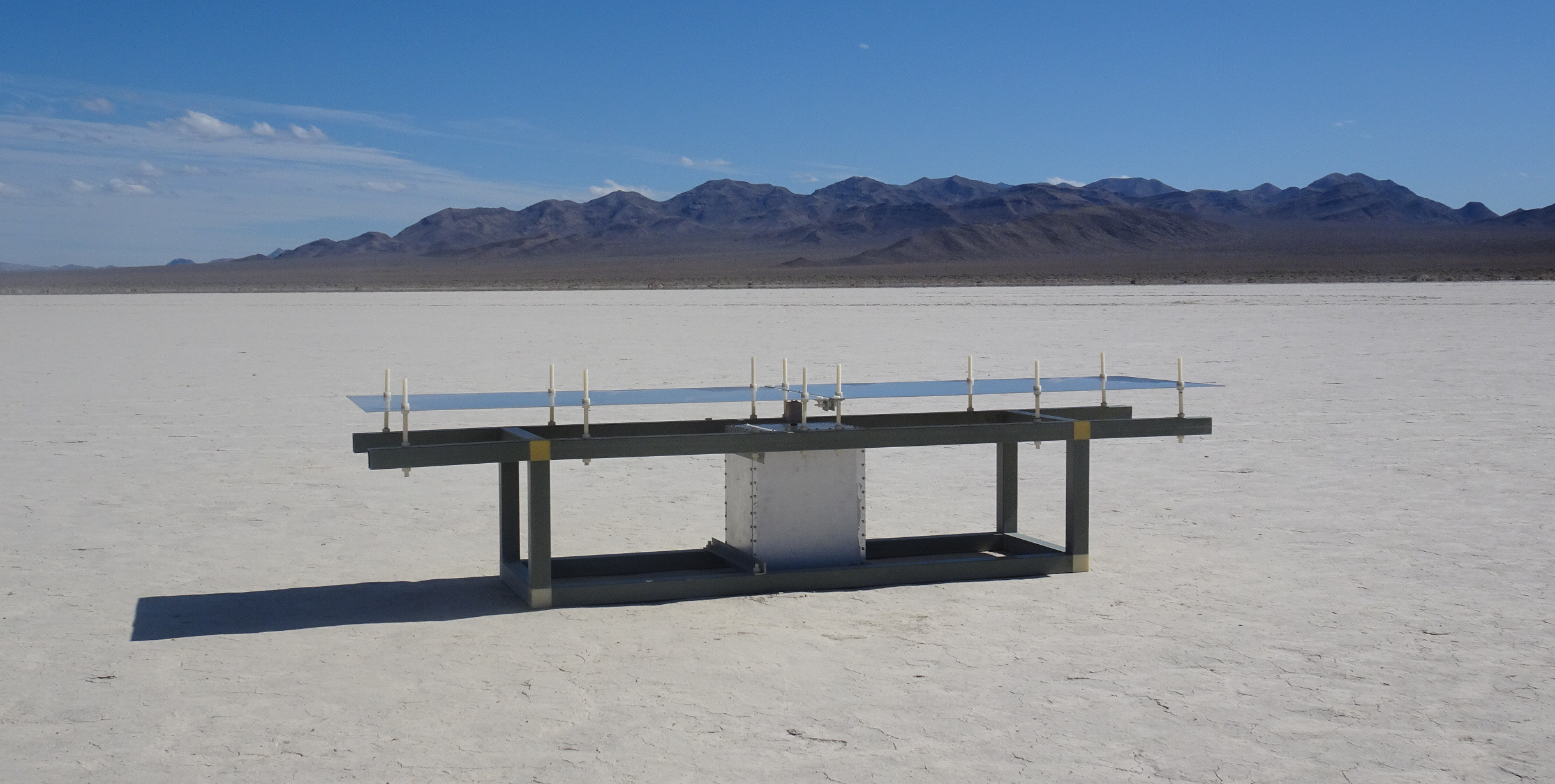
Figure 1: One of the two MIST instruments during sky observations in Death Valley, Nevada, in May 2022.

2 General description

The MIST instrument is a single-antenna, single-polarization, total power radiometer. The design of the instrument is motivated by the following objectives:

1. Have an antenna beam pattern above the soil that peaks at the zenith and decreases toward the horizon. This pattern would maximize the sensitivity of the instrument to the sky signal, and minimize the sensitivity to features of the terrain and sky blockage by mountains (Bassett et al., 2021).

2. Avoid using a metal ground plane. In addition to reducing the probability of instrumental resonances (Bradley et al., 2019), this choice would eliminate the possibility of signal reflections produced by the electrical discontinuity between the edges of the ground plane and the soil (Mahesh et al., 2021; Spinelli et al., 2022; Rogers et al., 2022). Operating without a ground plane increases the ground loss. However, the ground loss can in principle be estimated using electromagnetic simulations and then removed during data analysis. Observations from different sites could be leveraged to test for systematic effects related to ground loss.

3. Keep the instrument small and of low power consumption. These characteristics would enable the operation of the instrument with small batteries and facilitate its transportation to remote sites. In a small instrument, the radio-frequency (RF) paths would be short, increasing the accuracy with which key calibration parameters, in particular of the receiver, could be measured.

4. Avoid using cables outside of the receiver box. By avoiding cables we would eliminate their potential impact on the antenna performance, reduce emission of self-generated RFI, and simplify the design for electromagnetic simulations.

From the guidelines above, we arrived at a design based on a horizontal $2.42$ m tip-to-tip blade dipole antenna made of solid aluminum panels. The antenna operates $52$ cm above the soil and without a metal ground plane. The instrument is powered by four $12$ V, $18$ Ah batteries, and has a maximum power consumption of $17$ W. Except for a small balun, all the electronics of the instrument, including the batteries, are contained in a single aluminum receiver box of size $40.5$ cm $\times$ $33.5$ cm $\times$ $26$ cm located under the antenna. The antenna and receiver box are supported by a frame made of fiberglass tubes and angles, acrylonitrile butadiene styrene (ABS) plastic elbows, and nylon rods, screws, and nuts. The full frequency range of the radiometer is $0$–$125$ MHz but the sky observations are limited to the range $25$–$105$ MHz. The high-frequency end of this range is imposed by the reduced performance of the analog-to-digital converter (ADC) above $105$ MHz. The low-frequency end of the range is imposed by the reduced efficiency of the antenna combined with a significant increase in the shortwave RFI below $25$ MHz at most locations. The average FWHM of the antenna beam directivity across $25$–$105$ MHz is $\approx 85^{\circ}$.

Figure 1 shows a picture of one of the instruments deployed in Death Valley in May 2022. Figure 2 shows a schematic of the instrument and Table 1 lists the instrument’s dimensions.

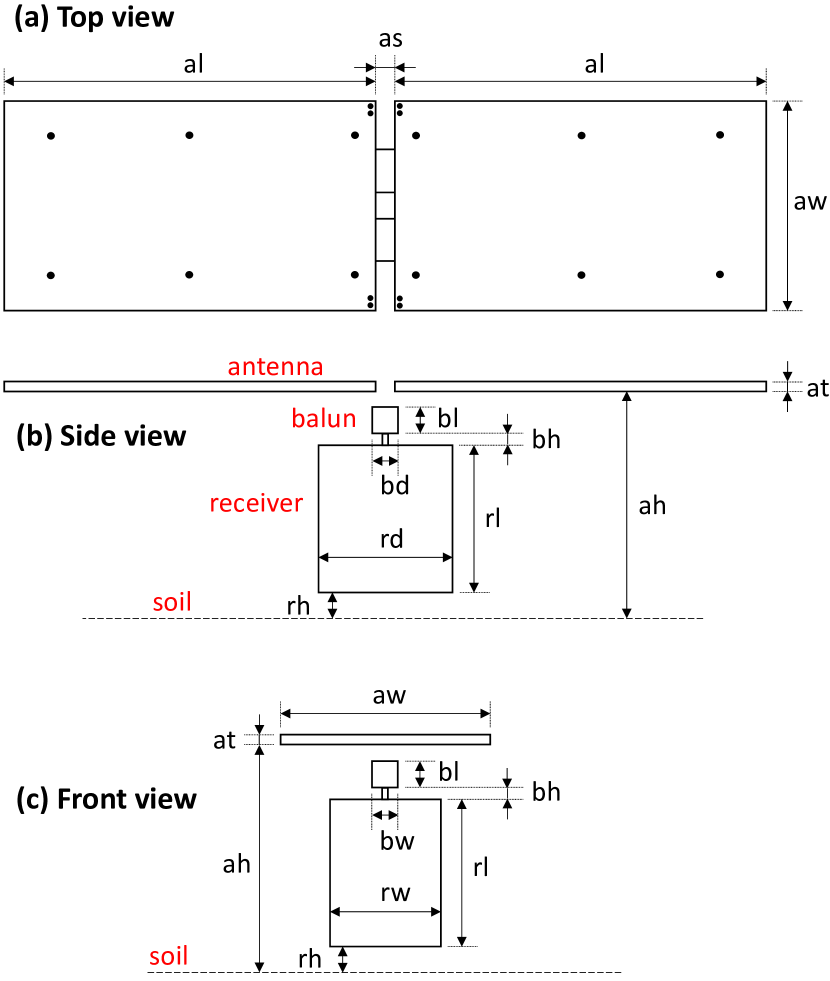
Figure 2: Schematic of the MIST instrument (not to scale). The dimensions are listed in Table 1.

3 Calibration formalism

Before describing the instrument in detail, here we summarize the mathematical model used by MIST for the sky measurements.

3.1 Sky contribution to the antenna temperature

The contribution from the sky to the antenna temperature is given by

$$T_{S}(\nu)=\frac{\int_{0}^{2\pi}\int_{0}^{\pi/2}T_{sky}(\theta,\phi,\nu)D(\theta,\phi,\nu)\sin\theta d\theta d\phi}{\int_{0}^{2\pi}\int_{0}^{\pi/2}D(\theta,\phi,\nu)\sin\theta d\theta d\phi},$$ (2)

where $T_{sky}$ is the sky brightness temperature spatial distribution; $D$ is the antenna beam directivity; $\theta$ and $\phi$ are the antenna zenith and azimuth angles, respectively; and $\nu$ is frequency.

The antenna temperature measured at the input of the calibrated receiver is modeled as

$$T_{A}(\nu)=\eta(\nu)T_{S}(\nu)+\left[1-\eta(\nu)\right]T_{phys},$$ (3)

where $\eta$ is the efficiency in the measurement of $T_{S}$ accounting for passive sources of loss, and $T_{phys}$ is the physical temperature associated with the passive sources of loss. MIST’s on-sky efficiency corresponds to the multiplication of three factors: (1) the radiation efficiency, $\eta_{rad}$, which accounts for resistive loss due to finite electrical conductivity in and around the antenna; (2) the beam efficiency, $\eta_{beam}$, which corresponds to the fraction of the beam solid angle toward the sky relative to the total; and (3) the balun efficiency, $\eta_{balun}$, representing the efficiency of the signal transmission through the balun used between the antenna excitation port and the receiver input. Assuming the same physical temperature for the three passive sources of loss, which typically corresponds to the ambient temperature, Equation 3 can be solved for the sky contribution to obtain

$$T_{S}=\frac{T_{A}-\left[1-\eta_{rad}\eta_{beam}\eta_{balun}\right]T_{phys}}{\eta_{rad}\eta_{beam}\eta_{balun}}.$$ (4)

3.2 Receiver calibration

The antenna temperature calibrated at the receiver input is related to the power spectral density (PSD) measured by the receiver, $P_{A}$, by

$$T_{A}(\nu)=\frac{P_{A}(\nu)}{g_{R}(\nu)}-T_{R}(\nu),$$ (5)

where $g_{R}$ is the receiver gain and $T_{R}$ is the receiver temperature. We determine $g_{R}$ and $T_{R}$ with the method developed in Rogers & Bowman (2012) and Monsalve et al. (2017a). In this method, the receiver input is continuously switched in the field between three positions: (1) the antenna, (2) an internal ambient load, and (3) the internal ambient load in series with an active noise source. In addition, external calibration standards of different noise temperatures and reflection coefficients are measured in the lab. These external standards provide the absolute calibration to the receiver. With some rearrangement of the PSD equations for the three receiver input positions presented in Monsalve et al. (2017a), $g_{R}$ and $T_{R}$ can be written as (dropping the frequency dependences of all the quantities for brevity)

$$g_{R} =\left(\frac{1}{K_{0}}\right)\left[\frac{P_{L+NS}-P_{L}}{C_{1}\left(T^{a}_{L+NS}-T^{a}_{L}\right)}\right],$$ (6)

$$T_{R}= K_{0}\Biggl{\{}P_{L}\left[\frac{C_{1}\left(T^{a}_{L+NS}-T^{a}_{L}\right)}{P_{L+NS}-P_{L}}\right]-(T^{a}_{L}-C_{2})\Biggl{\}}$$

$$+K_{U}T_{U}+K_{C}T_{C}+K_{S}T_{S}.$$ (7)

Here, $P_{L}$ and $P_{L+NS}$ are the PSDs from the internal ambient load and ambient plus noise source, respectively; $T^{a}_{L}$ and $T^{a}_{L+NS}$ are assumed values for the noise temperatures of the internal ambient load and ambient plus noise source, respectively; $C_{1}$ is an absolute multiplicative correction to the difference $T^{a}_{L+NS}-T^{a}_{L}$; $C_{2}$ is an absolute additive correction to $T^{a}_{L}$; and $T_{U}$, $T_{C}$, and $T_{S}$ are the noise wave parameters of the receiver front-end in the formalism of Meys (1978). $C_{1}$, $C_{2}$, $T_{U}$, $T_{C}$, and $T_{S}$ are referred to as the absolute receiver calibration parameters, which we determine using the measurements from the external calibration standards (Monsalve et al., 2017a). The $K$ parameters in Equations 6 and 7 capture the impedance mismatch between the antenna and the receiver input, and are given by:

$$K_{0} =\frac{1-|\Gamma_{R}|^{2}}{\left(1-|\Gamma_{A}|^{2}\right)|F|^{2}},$$ (8)

$$K_{U} =\frac{|\Gamma_{A}|^{2}}{1-|\Gamma_{A}|^{2}},$$ (9)

$$K_{C} =\frac{|\Gamma_{A}|}{\left(1-|\Gamma_{A}|^{2}\right)|F|}\cos\alpha,$$ (10)

$$K_{S} =\frac{|\Gamma_{A}|}{\left(1-|\Gamma_{A}|^{2}\right)|F|}\sin\alpha,$$ (11)

$$F =\frac{\sqrt{1-|\Gamma_{R}|^{2}}}{1-\Gamma_{A}\Gamma_{R}},$$ (12)

$$\alpha =\mathrm{arg}(\Gamma_{A}F),$$ (13)

where $\Gamma_{A}$ is the reflection coefficient of the antenna, including the effect of the balun, and $\Gamma_{R}$ is the reflection coefficient looking into the receiver input.

4 Antenna

Similarly to other experiments (e.g., Cummer et al., 2022; Anstey et al., 2022), in MIST we explored a variety of antenna types. In addition to having a zenith-pointing beam (Section 2), the antenna must produce a good impedance match with the receiver (Section 3.2) and have a geometry that is easy to simulate electromagnetically. After considering the tradeoffs between these criteria, we selected a horizontal blade dipole antenna for MIST.

The blade dipole antenna was introduced for global $21$ cm measurements by EDGES-2 in Mozdzen et al. (2016). However, in MIST we use this antenna without a ground plane, which represents a significant difference. Moreover, in MIST all the dimensions of the antenna and instrument (Table 1) are different from those in EDGES. These differences offer a valuable opportunity for the cross-checking of systematics between MIST and EDGES. The differences between MIST and other current experiments are even more substantial. In particular, SARAS uses a vertical monopole over water (Singh et al., 2022) and REACH uses two antenna types: a hexagonal dipole and a conical log-spiral, both above a $20$ m $\times$ $20$ m metal ground plane that is suspended above the soil (de Lera Acedo et al., 2022). With its unique characteristics, the MIST antenna represents a significant contribution to the experimental parameter space of global $21$ cm instruments.

Table 1: Dimensions of the MIST instrument. The parameters correspond to those in the schematic of Figure 2.

Dimension	Parameter	Value [m]
antenna panel length	al	$1.2$
antenna panel width	aw	$0.6$
antenna panel thickness	at	$0.003$
antenna panel separation	as	$0.02$
antenna panel height	ah	$0.52$
receiver length	rl	$0.405$
receiver width	rw	$0.26$
receiver depth	rd	$0.335$
receiver height	rh	$0.02$
balun length	bl	$0.05$
balun width	bw	$0.03$
balun depth	bd	$0.037$
balun height	bh	$0.022$

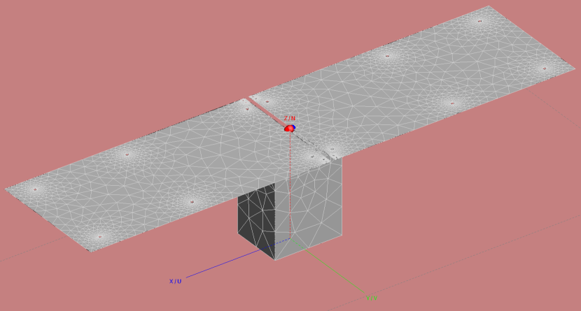
Figure 3: Screenshot of the FEKO electromagnetic simulations.

4.1 Electromagnetic simulations

We use electromagnetic simulations with the FEKO software to predict the parameters of the MIST antenna necessary for the calibration of the sky measurements —radiation efficiency, beam directivity, beam efficiency, and reflection coefficient (Section 3). In FEKO, we use the method of moments solver, which is the most suited for radiation problems involving electrically large structures.

4.1.1 Simulation geometry

The simulation geometry includes the antenna panels, balun, and receiver box, following the schematic of Figure 2 and dimensions of Table 1. The geometry also includes soil, which extends to infinity in the horizontal direction and depth. Figure 3 shows a screenshot of the simulations. The antenna panels are modeled as $3$ mm thick aluminum sheets. Each panel includes the holes illustrated in Figure 2: six of these holes connect to the support frame, and the four holes near the edge are used to fine-tune the panel-to-panel separation distance. The excitation port is simulated as a voltage source in the middle of a wire connecting the two antenna panels. The diameter of the wire is $1$ mm, which matches the diameter of the real wires that connect the antenna to the balun (Section 5). The simulated wire is modeled as a perfect electric conductor because the effect of the finite conductivity of the real wires is included in the S-parameters of the balun. The balun and receiver box are modeled as hollow boxes with $1.6$ mm thick aluminum walls, matching the real instrument. We use an electrical conductivity of $3.816\times 10^{7}$ Sm^-1 for aluminum (Gardiol, 1984). The antenna support frame (made out of fiberglass, nylon, and ABS plastic) does not have a significant effect on the antenna response and is not included in the simulations.

4.1.2 Soil models

The performance of the antenna depends very strongly on the electrical parameters of the soil: specifically, the conductivity ($\sigma$) and relative permittivity ($\epsilon_{r}$). In real soils, $\sigma$ and $\epsilon_{r}$ are spatially inhomogeneous. However, in FEKO it is only possible to design infinite soil models with variations as a function of depth. These variations are implemented using horizontal layers of different $\sigma$ and $\epsilon_{r}$ (Spinelli et al., 2022). To simplify the modeling and work within the capabilities of FEKO, for MIST we must choose observation sites where the soil is very close to flat and any variations primarily occur as a function of depth.

To explore the effect of soil on the MIST antenna performance, we run FEKO simulations with nine models for the soil. The characteristics of the models are listed in Table 2. Five of these models, labeled “nominal” and 1L_xx, are single-layer models. These models intend to mimic the optimistic scenario in which, from the point of view of the antenna, the soil can be well described as effectively uniform. The nominal model, which in this paper is used as a reference, has values $\sigma_{1}=0.01$ Sm^-1 and $\epsilon_{r1}=6$. In the 1L_xx models, the value of one of the parameters is changed relative to the nominal model, with the xx part of the label being used to identify the change. Specifically, c+ (c-) corresponds to an increase (decrease) in conductivity to $0.1$ ($0.001$) Sm^-1, and p+ (p-) represents an increase (decrease) in relative permittivity to $10$ ($2$). The values we use for $\sigma$ and $\epsilon_{r}$ fall within the ranges reported for several geological materials that we could encounter at our observation sites. For instance, snow and freshwater ice typically have $0\lesssim\sigma\lesssim 0.01$ Sm^-1 and $2\lesssim\epsilon_{r}\lesssim 6$. For sand, silt, and clay, $\sigma$ and $\epsilon_{r}$ strongly depend on moisture level and span the wide ranges $10^{-7}$–$10^{0}$ Sm^-1 and $2$–$40$, respectively (Reynolds, 2011). Our choices for the parameter values, in particular, closely match the values reported by Sutinjo et al. (2015) for the soil at the Inyarrimanha Ilgari Bundara, the CSIRO Murchison Radio-astronomy Observatory, with different moisture levels. Our values are also consistent with the soil measurements done by Spinelli et al. (2022) at the Owens Valley Radio Observatory for dry and wet conditions.

As shown in Table 2, our last four soil models, labeled 2L_xx, are two-layer models. The purpose of these models is to represent the more realistic situation in which there is a change in the soil parameters at some depth from the surface. In these models, the top layer has a thickness $L=1$ m and the same conductivity and permittivity as the nominal case, while the bottom layer extends to infinite depth and has a different value of either conductivity or permittivity. In each case, the parameter change made to the bottom layer is indicated in the model name, similarly to the single-layer models. Furthermore, the conductivity and relative permittivity values assigned to the bottom layer in the c+, c-, p+, and p- cases are the same as for the single-layer models. As an example, one observation site where the soil could be well represented by a two-layer model is MARS during the summer. At that site, the soil in the summer consists of an unfrozen top layer and a permanently frozen, or “permafrost”, bottom layer (e.g., Pollard et al., 2009; Wilhelm et al., 2011). We leave for future work the exploration of a wider range of soil models, including models with more than two layers (which were studied in Spinelli et al. (2022) for the LEDA experiment), and models that account for the fact that in real soils the conductivity and permittivity vary as a function of frequency (e.g., Revil, 2013).

4.1.3 Simulation settings

The simulations are conducted in the range $25$–$125$ MHz with a resolution of $1$ MHz. Although the sky measurements are currently analyzed up to $105$ MHz, the simulations extend up to $125$ MHz anticipating a future increase in the bandwidth of MIST. In FEKO, we use the fine mesh size setting and double-precision calculations. Using the $64$ cores of an AMD Ryzen Threadripper PRO 5995WX processor, each simulation takes $\approx 60$ minutes.

Next, we describe the results of the FEKO simulations for the radiation efficiency, beam directivity, beam efficiency, and reflection coefficient at the dipole excitation port.

Table 2: Soil models used in the FEKO simulations of MIST. Five of these models are single-layer models (“nominal” and 1L_xx) and four are two-layer models (2L_xx). The layers are characterized in terms of their electrical conductivity ($\sigma$) and relative permittivity ($\epsilon_{r}$). In the two-layer models, the thickness of the top layer is $L=1$ m.

Model	# layers	$\sigma_{1}$ [Sm-1]	$\epsilon_{r1}$	$\sigma_{2}$ [Sm-1]	$\epsilon_{r2}$
nominal	1	$0.01$	$6$
1L_c+	1	$0.1$	$6$
1L_c-	1	$0.001$	$6$
1L_p+	1	$0.01$	$10$
1L_p-	1	$0.01$	$2$
2L_c+	2	$0.01$	$6$	$0.1$	$6$
2L_c-	2	$0.01$	$6$	$0.001$	$6$
2L_p+	2	$0.01$	$6$	$0.01$	$10$
2L_p-	2	$0.01$	$6$	$0.01$	$2$

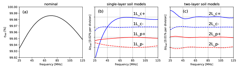
Figure 4: (a) Radiation efficiency for the nominal soil model. (b) and (c) Differences in radiation efficiency between the alternative soil models and the nominal model. For example, for model 1L_c+, $\Delta\eta_{rad}=\eta_{rad,\;\texttt{1L\_c+}}-\eta_{rad,\;nominal}$. In panels (b) and (c), the zero-points for the differences are the labeled horizontal grid lines.

4.2 Radiation efficiency

The radiation efficiency of the antenna, $\eta_{rad}$, is defined as the ratio of radiated power to input power. $\eta_{rad}$ relates the beam gain, $G$, to the beam directivity by

$$G(\theta,\phi,\nu)=\eta_{rad}(\nu)D(\theta,\phi,\nu).$$ (14)

In this definition, the efficiency only considers resistive, or “ohmic”, loss in the antenna and conductive regions visible to the antenna, and not impedance mismatch or external losses, such as ground loss (Stutzman & Thiele, 1998). In our FEKO simulations, we assign the finite conductivity of aluminum to the antenna panels, balun, and receiver box, and the conductivities of Table 2 to the soil. This information enables FEKO to calculate and directly provide $\eta_{rad}$ and $G$. The beam directivity is a derived quantity and obtained from $\eta_{rad}$ and $G$ (Section 4.3).

Figure 4 shows the radiation efficiency for the nine FEKO simulations. Panel (a) shows that for the nominal soil model, the efficiency is in the range $99.93\%$–$99.99\%$ and has a smooth frequency dependence. This high efficiency is expected for the high conductivity of the instrument’s aluminum surfaces. Panels (b) and (c) show the difference in the radiation efficiency for the alternative soil models relative to the nominal model. The main takeaway of these panels is the confirmation that the radiation efficiency is sensitive to the characteristics of the soil, in addition to those of the instrument’s surfaces. For our single-layer (two-layer) models, the largest change is $\approx 0.08\%$ ($\approx 0.007\%$). Although small compared to the total efficiency, these changes are comparable to, or larger than, the ratio between the global $21$ cm signal and the diffuse astrophysical foreground, which is $\approx 0.01\%$ for the Cosmic Dawn and smaller for the Dark Ages. This comparison highlights the need to accurately determine and account for the radiation efficiency in order to minimize biases in the $21$ cm signal estimation.

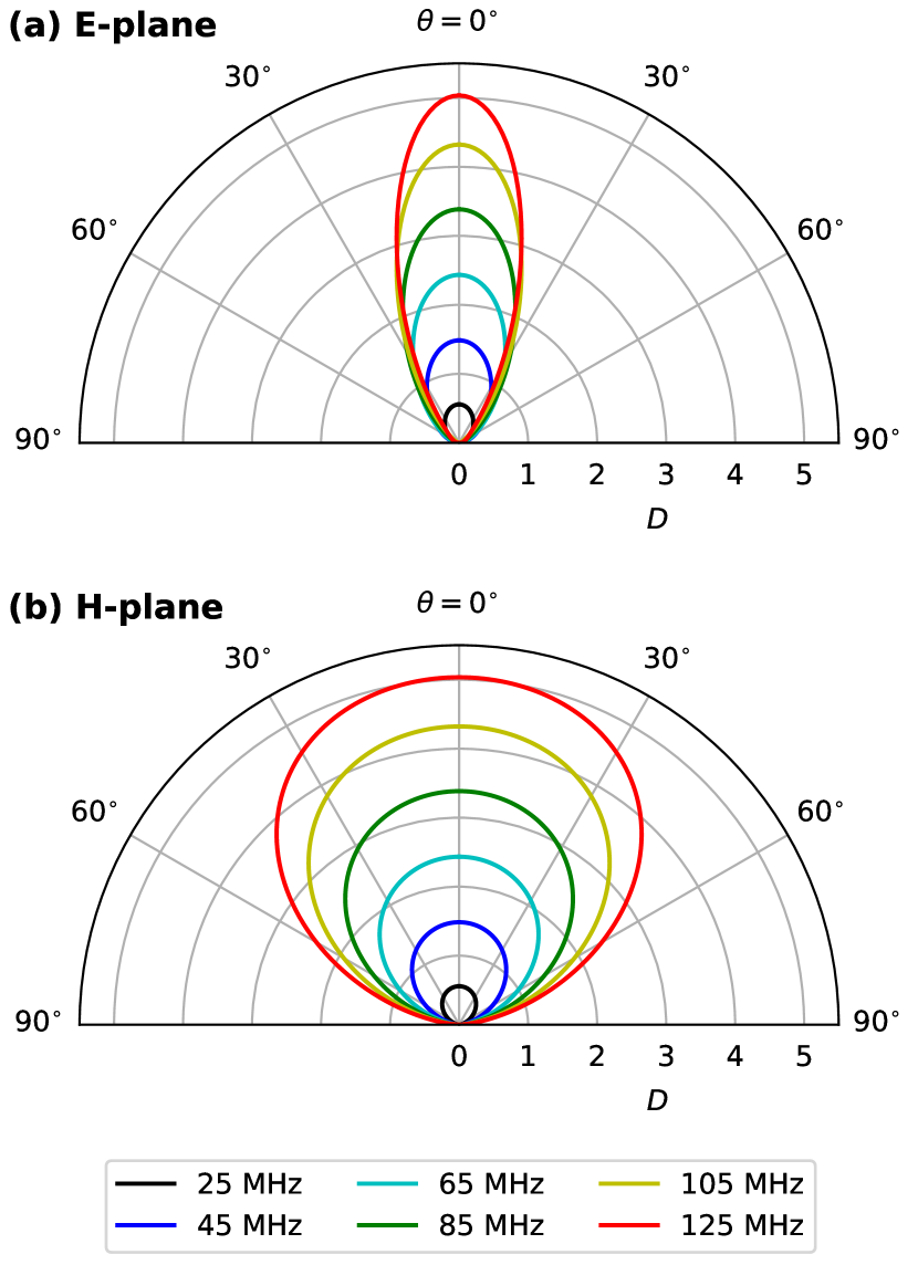
Figure 5: Antenna beam directivity for the nominal soil model in the E- and H- planes at six frequencies.

4.3 Beam directivity

We compute the beam directivity as $D=\eta_{rad}^{-1}$G using the gain and radiation efficiency provided by FEKO. The directivity is only computed for the top hemisphere because FEKO cannot provide the gain in the soil when the soil has non-zero electrical conductivity. In MIST, the effect of the directivity in the soil is accounted for through the beam efficiency, which is calculated using the top-hemisphere directivity (Section 4.4).

Figure 5 shows slices of the directivity every $20$ MHz for the nominal soil model. The slices are shown for the E- and H- planes, which are parallel and perpendicular to the antenna excitation axis (i.e., the antenna’s length), respectively. The directivity peaks at the zenith and is minimized at the horizon, satisfying one of the main design objectives for the antenna (Section 2). The peak directivity increases monotonically from $\approx 0.6$ to $\approx 5.1$ between $25$ and $125$ MHz, and the directivity pattern is wider in the H-plane at all frequencies.

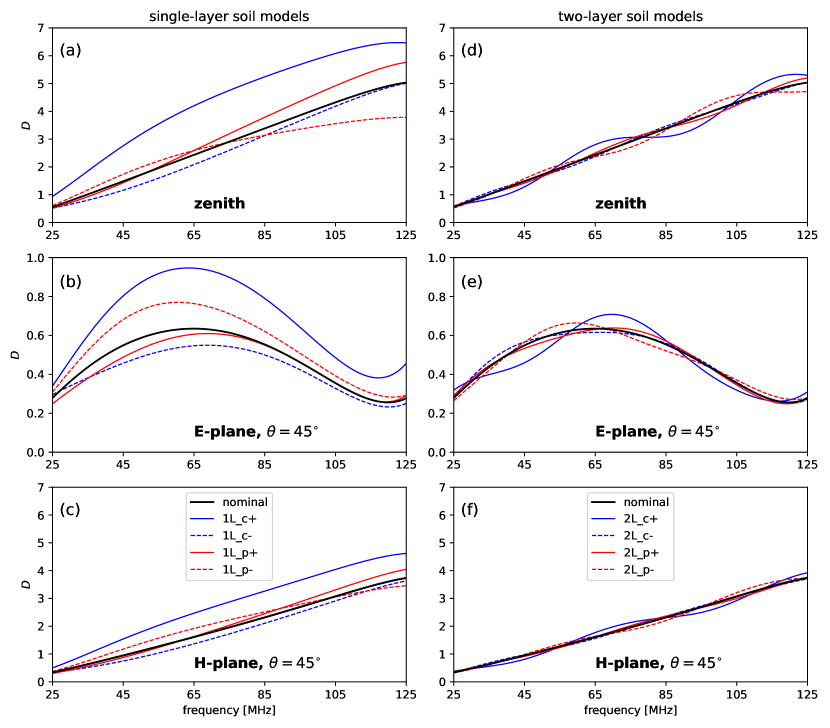
Figure 6: Antenna beam directivity for all the soil models at three reference puncture points: (top row) zenith; (middle row) E-plane at $\theta=45^{\circ}$; and (bottom row) H-plane at $\theta=45^{\circ}$.

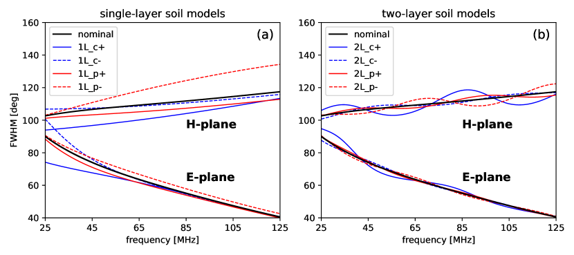
Figure 7: FWHM of the antenna beam directivity in the E- and H-planes for all the soil models.

Figure 6 shows the directivity for the nine soil models at three reference puncture points: (1) the zenith, (2) the E-plane at $\theta=45^{\circ}$, and (3) the H-plane at $\theta=45^{\circ}$. In this figure, we identify the following important points:

1. The directivity is very sensitive to the properties of the soil. As expected, the effects are larger when the changes in the soil extend all the way to the surface, which occurs in the single-layer models. For these models, the directivity increases with conductivity across most of the frequency range. In particular, the directivity for model 1L_c+ is $>20\%$, and at some frequencies $>50\%$, higher than the nominal. Changes in permittivity also produce significant changes in the directivity, but the sign of the changes evolves with frequency.

2. The uniformity of the single-layer soil models results in a directivity that is relatively smooth across frequency. For two-layer models, changes in the bottom layer introduce ripples which, for the $1$ m thickness of the top layer, have a period of $\approx 50$ MHz.

3. At the zenith and the H-plane puncture point, the directivity increases with frequency for all soil models to values that, at the highest frequencies, are $>3$. At the E-plane puncture point, the directivity is always $<1$ and peaks at $\approx 55$–$75$ MHz. The directivities at the E- and H-plane puncture points indicate that the beam is wider in the H-plane for all the soil models.

As a direct quantification of the beam width, Figure 7 shows the FWHM of the directivity pattern in the E- and H-planes for the nine soil models. For all the models, the FWHM is larger in the H-plane than in the E-plane. Moreover, in the H-plane the FHWM increases with frequency while in the E-plane it decreases. For our soil models, the H-plane FWHM is in the range $85^{\circ}$–$107^{\circ}$ at $25$ MHz, increasing to $113^{\circ}$–$135^{\circ}$ at $125$ MHz. In the E-plane, the FWHM is in the range $74^{\circ}$–$101^{\circ}$ at $25$ MHz, decreasing to $39^{\circ}$–$43^{\circ}$ at $125$ MHz. In both planes, the FWHM increases with decreasing permittivity at the soil surface, as seen when comparing single-layer cases 1L_p+ and 1L_p- with the nominal. Similarly to the directivity (Figure 6), the frequency evolution of the FWHM for the single-layer models is relatively smooth. For the two-layer models, the FWHM shows ripples with a period of $\approx 50$ MHz and a peak amplitude of up to $\approx 8^{\circ}$ with respect to the nominal model. The amplitude of the ripples is larger in the H-plane than in the E-plane.

The beam directivity of a global $21$ cm instrument has a very strong impact on the accuracy of the signal recovery (e.g., Mahesh et al., 2021; Anstey et al., 2022; Cummer et al., 2022; Spinelli et al., 2022). In a future paper (Monsalve et al., in prep.), we will discuss the $21$ cm signal extraction accuracy expected for the MIST beam directivity and different soil characteristics.

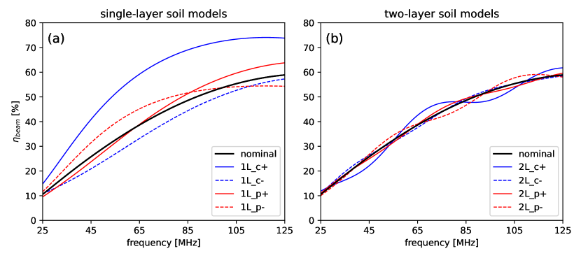
Figure 8: Beam efficiency for all the soil models.

4.4 Beam efficiency

We define the beam efficiency, $\eta_{beam}$, as the solid angle of the beam directivity in the top hemisphere divided by the solid angle over the full sphere, i.e.,

$$\eta_{beam}(\nu)=\frac{1}{4\pi}\int_{0}^{2\pi}\int_{0}^{\pi/2}D(\theta,\phi,\nu)\sin\theta d\theta d\phi.$$ (15)

This efficiency is equivalent to one minus the ground loss fraction. Figure 8 shows the beam efficiency for the nine soil models. The main trend observed across models is an increase of the efficiency with frequency. The efficiency is in the range $9\%$–$15\%$ at $25$ MHz, increasing to $54\%$–$74\%$ at $125$ MHz. The efficiency also increases with the conductivity at the soil surface, as seen when comparing single-layer cases 1L_c+ and 1L_c- with the nominal. This dependence is consistent with intuition: the efficiency would be $100\%$ if the soil surface had infinite conductivity, or if an infinitely large and infinitely conducting ground plane were used. As expected from the directivity and FWHM plots (Figures 6 and 7), the beam efficiency has a relatively smooth frequency evolution for single-layer models, while for two-layer models it contains ripple-like structure. This structure has a period of $\approx 50$ MHz and a peak amplitude of up to $\approx 5\%$ with respect to the nominal model.

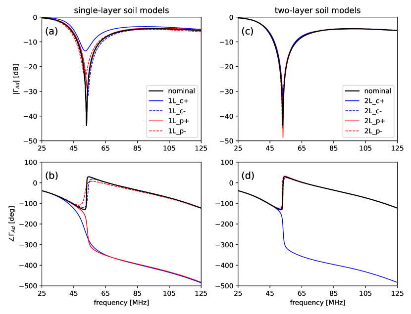
Figure 9: Reflection coefficient at the dipole excitation port for all the soil models.

4.5 Reflection coefficient at dipole excitation port

Our FEKO simulations provide the reflection coefficient of the antenna at the dipole excitation port, $\Gamma_{Ad}$. The reflection coefficient at the balun output, $\Gamma_{A}$, which is the quantity required for receiver calibration (Section 3.2), is described in Section 5.2.

Figure 9 shows $\Gamma_{Ad}$. At the excitation port, the main characteristic of the reflection magnitude (top row) is a resonant feature at $\approx 52$ MHz, where the magnitude reaches a minimum. From this resonance, the magnitude increases monotonically toward lower frequencies until it reaches $\approx 0$ dB at $25$ MHz. The magnitude also increases toward higher frequencies and has a peak of $\approx-4$ dB at $90$–$95$ MHz. For single-layer models, the reflection magnitude shows a strong dependence on soil parameters. The largest effect is at the resonance, where the magnitude varies from $\approx-15$ to $-45$ dB across our models. The soil parameters also affect the resonance frequency. Specifically, this frequency decreases with conductivity and increases with permittivity. For our models, these changes are within a few MHz. For two-layer models, changes in the bottom layer produce changes in reflection magnitude that are typically within $2$ dB, except at the resonance.

The bottom row of Figure 9 shows the reflection phase. The phase has a predominantly descending slope and a relatively fast $\approx 180^{\circ}$ transition at the resonance. Changes in the soil impact the phase primarily around the resonance. For most of our models, when going through the resonance from lower to higher frequencies the phase increases. However, for some models the phase decreases, leading to a $\approx 360^{\circ}$ difference across models above the resonance. The negative slope of the phase corresponds to the antenna delay. Except around the resonance, the delay is similar across our models. Specifically, the phase change between $25$ and $45$ MHz (below the resonance) is $\approx 60^{\circ}$, corresponding to a delay of $\approx(60^{\circ}/360^{\circ})\times(20\;\mathrm{MHz})^{-1}\approx 8\;\mathrm{ns}$. Between $55$ and $125$ MHz (above the resonance) the phase change is $\approx 150^{\circ}$ and the delay is $\approx 6$ ns.

4.6 Variation of top layer thickness

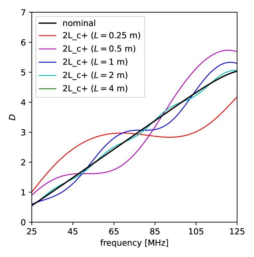
Figure 10: Ripples in the antenna beam directivity at the zenith for the 2L_c+ two-layer soil model. The only parameter being varied is the thickness of the top layer, $L$. The directivity for the nominal single-layer model is also shown for reference. Relative to the nominal directivity, as $L$ increases, both the amplitude and period of the ripples decrease. The directivity for $L=4$ m (green line) is not visible because it is almost perfectly overlapped by the nominal directivity. The dependence of the ripples on $L$ observed in this example is, qualitatively, representative of the other antenna parameters discussed in Section 4.

So far, the results we have shown for two-layer soil models correspond to cases in which the thickness of the top layer is $L=1$ m. Here, we present one example of how the ripples produced by two-layer models change when the top layer thickness is varied in the range $0.25$–$4$ m. For this example, we use the 2L_c+ model because it is the one that, among our two-layer models with $L=1$ m, produces the largest ripples, making the results easier to see and interpret. In this example, we only show the beam directivity at the zenith, which qualitatively represents the behavior of the ripples in the other antenna parameters. The results are shown in Figure 10. As the top layer thickness increases, the period of the ripples in the directivity decreases. This occurs because of the increased delay of the signal reflected back to the antenna from the interface between the two layers. As $L$ increases, the amplitude of the ripples also decreases. This is due to the increased attenuation suffered by the reflected signal as it travels a larger round-trip distance through the lossy top layer.

5 Balun

5.1 Description

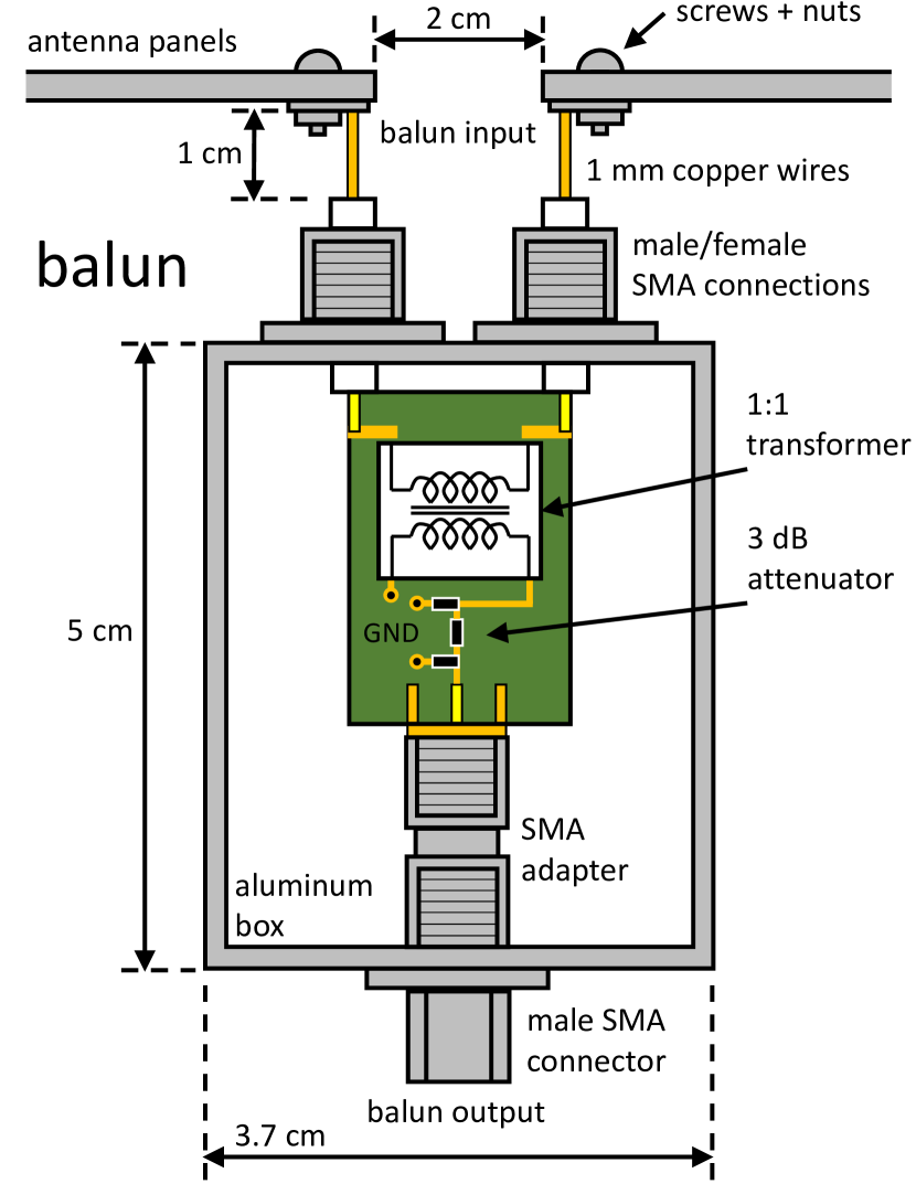
Figure 11: Side view schematic of the balun (not to scale). The core components are a 1:1 $50$ $\Omega$ transformer and a $3$ dB attenuator, which are housed inside the aluminum box.

We use a passive balun to convert the balanced signal produced at the excitation port of the dipole antenna to unbalanced, or ground-referenced, which is how the signal is expected at the receiver input. Figure 11 shows a schematic of the balun. The balun primarily consists of a Mini-Circuits TX1-1+ 1:1 $50$ $\Omega$ transformer in series with a $\approx 3$ dB attenuator on the unbalanced side. The transformer provides DC isolation and magnetic coupling between the balanced and unbalanced sides. The attenuator reduces the magnitude of the antenna reflection coefficient seen by the receiver input, which makes the calibrated sky measurements less sensitive to errors in reflection coefficient measurements (Monsalve et al., 2017a). The improved impedance matching from the attenuator comes at a cost of increased signal loss. However, this loss can be accurately measured in the laboratory and subsequently corrected in the sky measurements. To minimize the sensitivity of the balun to temperature fluctuations, the attenuator is constructed with resistors that are temperature-stable to better than $10$ ppm ^∘C^-1. On the balanced side of the balun, i.e., the balun input, the antenna panels are connected to the transformer through two $1$ cm long wires of $1$ mm diameter in series with male and female SMA connectors. The unbalanced side of the balun, i.e., the balun output, connects to the receiver input through a male SMA connector.

To characterize the balun, we measured its S-parameters in the lab. The measurements, which include the effect of the wires connecting the antenna panels to the transformer, are shown in Figure 12. These measurements were calibrated using a Keysight 85033E $3.5$ mm calibration kit. To increase the accuracy of this calibration, instead of using the nominal value of $50$ $\Omega$ for the impedance of the calibration load, we used the DC resistance of the load measured with a $5.5$-digit multimeter. Also, instead of assuming zero delay for the load’s transmission line, we used the delay estimated in Monsalve et al. (2016).

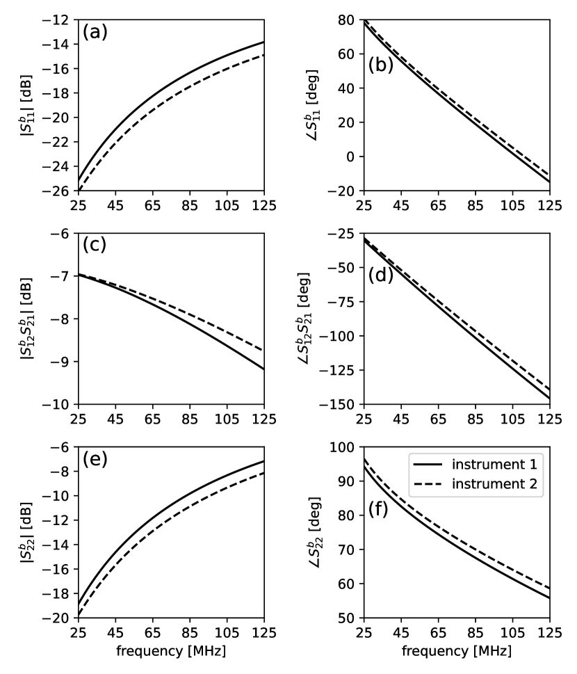
Figure 12: S-parameters of the MIST baluns measured in the lab. Here, port $1$ is the unbalanced port facing the receiver input (balun output) and port $2$ is the balanced port facing the antenna excitation port (balun input).

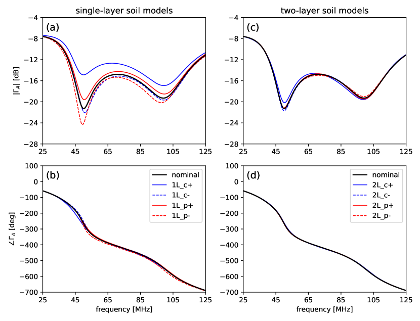
Figure 13: Reflection coefficient of the antenna at the balun output for all the soil models. Here, the plots show the simulated reflection coefficients from Figure 9 after embedding the measured balun S-parameters from instrument $1$ (Figure 12).

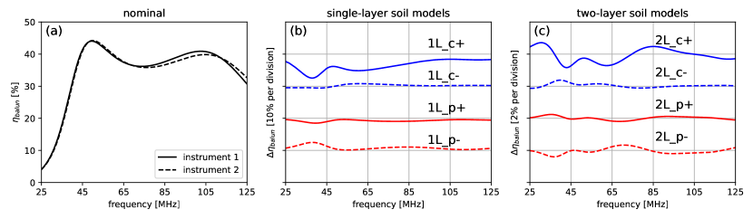
Figure 14: (a) Balun efficiency for the two MIST instruments computed with the antenna reflection coefficient for the nominal soil model. (b) and (c) Differences in balun efficiency for instrument $1$ between the alternative soil models and the nominal model. For example, for model 1L_c+, $\Delta\eta_{balun}=\eta_{balun,\;\texttt{1L\_c+}}-\eta_{balun,\;nominal}$. In panels (b) and (c), the zero-points for the differences are the labeled horizontal grid lines.

5.2 Antenna reflection coefficient at balun output

The antenna reflection coefficient at the balun output, $\Gamma_{A}$, is computed from the $\Gamma_{Ad}$ provided by FEKO (Section 4.5) using

$$\Gamma_{A}=S^{b}_{11}+\frac{S^{b}_{12}S^{b}_{21}\Gamma_{Ad}}{1-S^{b}_{22}\Gamma_{Ad}}.$$ (16)

In this equation, $S^{b}_{11}$, $S^{b}_{21}$, $S^{b}_{12}$, and $S^{b}_{22}$ are the S-parameters of the balun, with port 1 (2) being the balun output (input). The process represented by Equation 16 is referred to as “embedding” of S-parameters

Figure 13 shows $\Gamma_{A}$ computed for the nine soil models and the balun S-parameters from instrument $1$. The top row of the figure shows that the balun reduces the reflection magnitude relative to $|\Gamma_{Ad}|$ in Figure 9 across most of the frequency range, except for the resonance at $\approx 50$–$60$ MHz. As Equation 16 indicates, when $S^{b}_{11}$ and $S^{b}_{22}$ are low, the decrease in the magnitude is mainly driven by $|S^{b}_{12}S^{b}_{21}|$, which is $\approx-7$ to $-9$ dB (Figure 12). The soil differences between our single-layer models produce magnitude variations in the range $\approx-14$ to $-24$ dB at the $\approx 50$ MHz dip. For these models, the reflection magnitude increases with both conductivity and permittivity. For our two-layer models, soil changes below the surface lead to changes in reflection magnitude $\lesssim 2$ dB.

The bottom row of Figure 13 shows that the reflection phase at the balun output decreases monotonically across $25$–$125$ MHz. The transition at $\approx 50$ MHz is smoother than for $\angle\Gamma_{Ad}$ and there are no $360^{\circ}$ jumps. The phase variations across our single-layer (two-layer) models are $\lesssim 40^{\circ}$ ($\lesssim 10^{\circ}$). The delay of the antenna plus balun across $25$–$125$ MHz is $\approx(630^{\circ}/360^{\circ})\times(100\;\mathrm{MHz})^{-1}\approx 18\;\mathrm{ns}$. For comparison, the delay of the EDGES low-band antenna including the Roberts balun is $\approx 28$ ns (Bowman et al., 2018). A lower delay is preferred because it makes the calibrated sky measurements less sensitive to errors in reflection measurements (Monsalve et al., 2017a).

5.3 Balun efficiency

The balun efficiency is computed as (Monsalve et al., 2017a)

$$\eta_{balun}=\frac{|S^{b}_{12}|^{2}\left(1-|\Gamma_{Ad}|^{2}\right)}{|1-S^{b}_{22}\Gamma_{Ad}|^{2}\left(1-|\Gamma_{A}|^{2}\right)}.$$ (17)

Figure 14 shows the balun efficiency. Panel (a) shows the efficiency for both MIST instruments and the nominal soil model. For this model, the lowest efficiency is $\approx 5\%$ at $25$ MHz and the highest is $\approx 45\%$ at $50$ MHz. The shape of these curves strongly follows the magnitude of the reflection coefficient at the balun output (Figure 13), with higher efficiency occurring for lower reflection magnitude. Because the antenna reflection coefficient depends on the soil properties, so does the balun efficiency. Panels (b) and (c) of Figure 14 show the differences in efficiency for the alternative soil models relative to the nominal model with the balun of instrument $1$. The largest differences occur for the single-layer models and are of up to $\approx 8\%$. For the two-layer models, changes in the bottom layer produce efficiency changes of up to $\approx 0.8\%$. These differences are significantly larger than the $\lesssim 0.01\%$ ratio between global $21$ cm signal and astrophysical foreground, and have a spectral structure that could bias the $21$ cm signal extraction if not accounted for. It is thus necessary to compute the balun efficiency using high-accuracy in-situ measurements of the antenna reflection coefficient.

6 Receiver

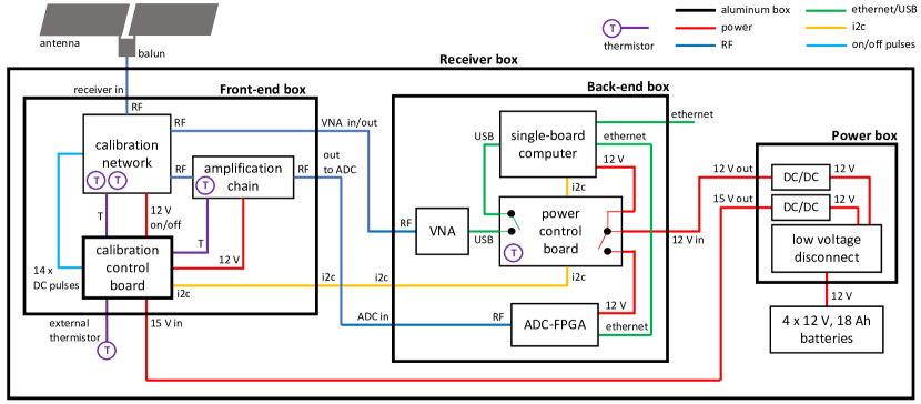
Figure 15: Block diagram of the MIST receiver.

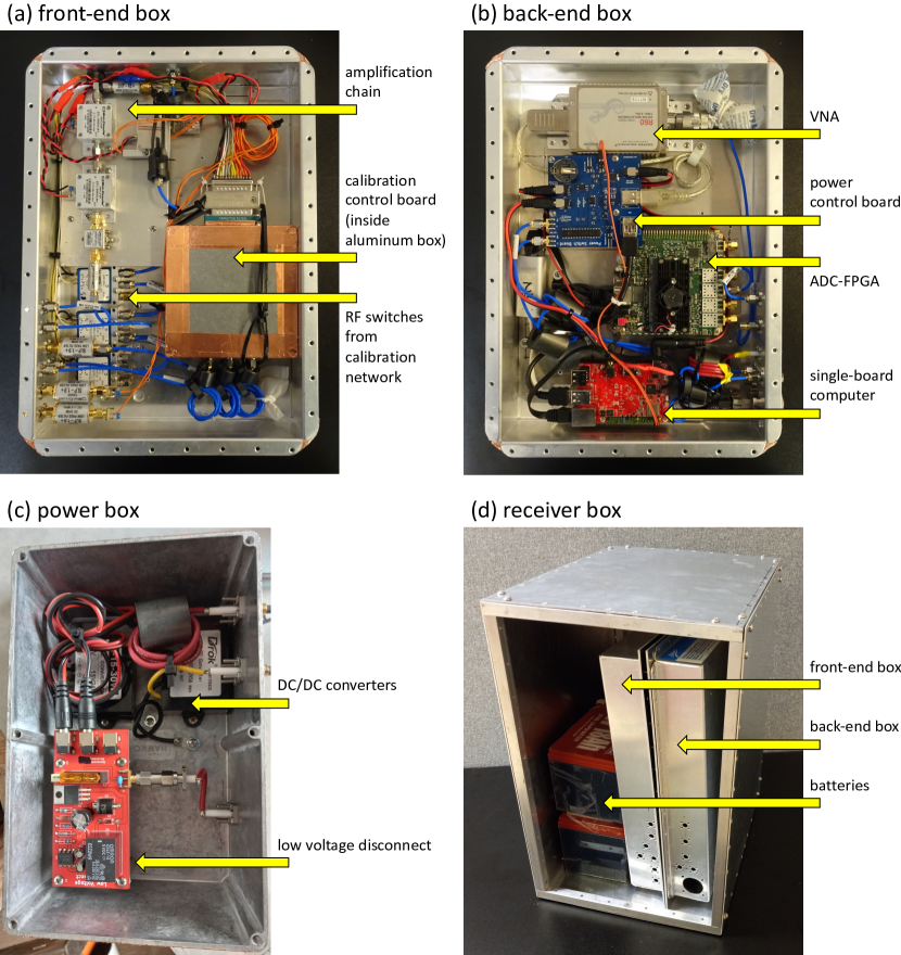
Figure 16: One of the MIST receivers: (a) front-end box; (b) back-end box; (c) power box; and (d) receiver box. The picture of the receiver box was taken during construction and assembly, and not all the features are shown. Three specific things not shown are: (1) the SMA input connector at the top of the box; (2) the plastic sleeves that protect the batteries; and (3) the power box, which sits above the batteries.

In this section, we describe the hardware and operation of the MIST receiver.

6.1 Overview

Figure 15 shows a block diagram of the receiver. Inside the receiver box, the electronics are housed in three boxes: the front-end box, the back-end box, and the power box. Figure 16 shows pictures of these boxes.

After leaving the balun, the antenna signal enters the front-end box. Here, the first subsystem encountered is the calibration network. This network contains calibration standards necessary for the implementation of our receiver calibration formalism (Section 3.2). The calibration network has two outputs; one to measure the antenna PSD, and the other to measure the reflection coefficient of the antenna and the reflection coefficient looking into the receiver input. From the PSD output, the signal goes through an amplification chain and is then routed to the back-end box. From the reflection output, the signal is routed directly to the back-end box. A calibration control board in the front-end box is used to provide the control signals required by the calibration network.

In the back-end box, the analog signal from the PSD output is digitized by an ADC and transformed to the frequency domain by a field-programmable gate array (FPGA). A single ADC-FPGA board performs both functions. The signal from the reflection output is measured by a vector network analyzer (VNA). A power control board is used to independently turn on and off the ADC-FPGA and VNA. A single-board computer (SBC) coordinates the PSD and reflection measurements, and also stores the data. To coordinate the measurements, the SBC controls the power control board in the back-end box and the calibration control board in the front-end box. An ethernet connection is used to communicate with the SBC from outside the back-end box.

The instrument is powered by four $12$ V, $18$ Ah batteries. Inside the power box, two DC/DC converters stabilize the fluctuating battery voltage to $15$ V and $12$ V. These voltages are used to power the front-end and back-end boxes, respectively. The power box also contains a low voltage disconnect (LVD) circuit to prevent the discharging of the batteries below safe levels.

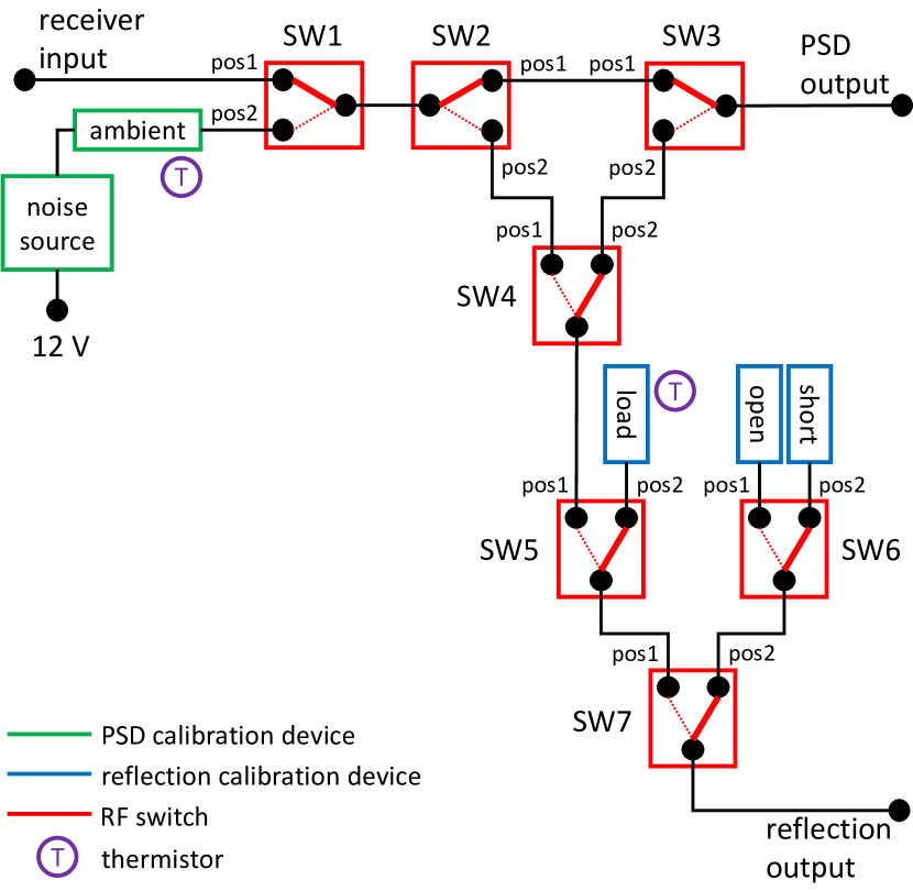
Figure 17: Diagram of the calibration network. The network is composed of calibration standards for PSD and reflection measurements, latching RF switches, and two thermistors.

6.2 Front-end box

6.2.1 Calibration network

Figure 17 shows the components of the calibration network. The network contains an ambient load and an active noise source for the calibration of PSD measurements (Section 3.2). The ambient load is implemented as two SMA attenuators ($20$ and $6$ dB) connected in series for a total attenuation of $26$ dB. These attenuators provide a noise temperature equivalent to their physical temperature (typically $\approx 300$ K). The noise source is built around a noise diode with an excess noise ratio of $\approx 35$ dB. When combined, the ambient load plus noise source provide a nominal noise temperature of $\approx$2,500 K, which is higher than the expected antenna temperature from sky measurements affected by losses (Equation 3). The noise temperature of the ambient load plus noise source was tuned to optimize the dynamic range of the ADC. The noise source is powered with $12$ V and only during the measurement of its PSD. The calibration network also contains open, short, and $50$ $\Omega$ load (OSL) standards for the calibration of reflection coefficient measurements. For the open and short we use commercially available SMA caps. The load is implemented using a $50$ $\Omega$ resistor that is temperature-stable to better than $10$ ppm ^∘C^-1. We use thermistors to measure the temperatures of the $20$+$6$ dB attenuators and the $50$ $\Omega$ resistor.

The network contains seven radio frequency (RF) switches (SW1 through SW7) to route the signals in the required directions. The RF switches are electromechanical, single-pole-double-throw, latching switches with SMA connectors. Switch SW1 selects between the receiver input (to which we connect the antenna plus balun or an external calibration device), and the internal ambient load and noise source. SW2 routes the output of SW1 either toward the PSD output or the reflection output. SW3 is used to switch the input of the amplification chain between two modes: PSD measurements through SW1 and SW2, and the measurement of the reflection coefficient looking into the amplification chain through SW4. Switch SW4 is also used to measure the reflection coefficient of the antenna, internal ambient, and ambient plus noise source, through SW1 and SW2. Switches SW5, SW6, and SW7 are used to measure the reflection coefficient of the OSL standards.

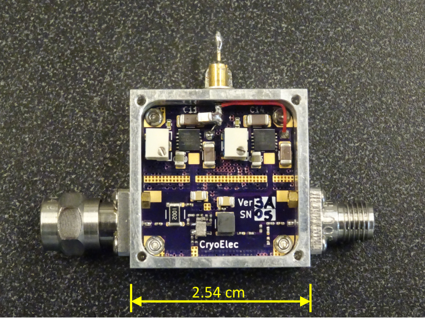
Figure 18: Custom LNA used by MIST.

6.2.2 Amplification chain

In PSD measurement mode, after leaving the calibration network, the signal from the receiver input (or internal ambient and noise source) reaches the amplification chain. The first elements in the chain are a $3$ dB attenuator and an LNA. The attenuator is used to improve the impedance match between the LNA and the antenna. The increased noise temperature due to this attenuator is small compared to the temperature from the astrophysical foregrounds which, aside from RFI, is the largest contributor to the system temperature when the receiver input is in the antenna position. Figure 18 shows a picture of the LNA. The LNA is a custom-made, silicon-germanium, heterojunction bipolar transistor design optimized for low reflections at the input and output ($|S_{11}|$ and $|S_{22}|<-35$ dB), as well as for low reverse transmission ($|S_{12}|<-40$ dB). The gain of the LNA is $\approx 28$ dB and its noise temperature is $\approx 150$ K. We measure the physical temperature of the LNA using a thermistor.

A $10$ dB attenuator is connected to the output of the LNA to improve the match between the LNA and the next components, as well as to regulate the total receiver gain. After the $10$ dB attenuator, a $48$ MHz high-pass filter is used to reduce incoming power from strong shortwave RFI. This filter is followed by two $\approx 20$ dB amplifiers, another $48$ MHz high-pass filter, and a $120$ MHz low-pass filter used to suppress RFI above the band, such as from ORBCOMM satellites, and contamination from aliased signals. We have not encountered the need to inject noise to the signal chain below the observation band (i.e., $<25$ MHz) for conditioning purposes, as performed by EDGES (Rogers & Bowman, 2012; Monsalve et al., 2017a; Bowman et al., 2018). The total nominal gain of the amplification chain is $\approx 55$ dB. The power consumption of the amplification chain is $2.5$ W.

6.2.3 Calibration control board

The calibration control board is used to generate the pulses that control the latching RF switches in the calibration network. These pulses have a voltage of $12$ V, a duration of one second, and are produced using MOSFET relays. The calibration control board also regulates and filters the $15$ V coming from the power box to produce the $12$ V used for the pulses. These $12$ V are also used to power the amplification chain and the noise diode. The calibration control board includes low-speed ADCs, which connect to the thermistors that measure the physical temperatures of the LNA, the internal calibration loads, and the external calibration devices.

6.3 Back-end box

6.3.1 ADC-FPGA

The ADC-FPGA used by MIST is a Koheron ALPHA250, which is powered with $12$ V and has a consumption of $10$ W. The board is built around a Zynq 7020 system-on-a-chip, which integrates an ARM Cortex-A9 processor and a Xilinx 7-series FPGA. The board has two RF ADCs and two RF digital-to-analog converters. MIST uses only one RF ADC. The analog signal coming out of the amplification chain is sampled by this ADC at a rate of $250\times 10^{6}$ samples per second and with an amplitude resolution of $14$ bits. The FPGA converts this digital signal to the frequency domain using an FFT algorithm with a Blackman-Harris window function. Each FFT computation uses 8,192 time samples and produces a PSD in the range $0$–$125$ MHz with a resolution of $30.518$ kHz.

6.3.2 Vector network analyzer

The VNA used by MIST is a Copper Mountain Technologies R60, which is powered through its USB connection and has a consumption of $3$ W. The reflection measurements with this VNA are done over the range $1$–$125$ MHz, with a resolution of $250$ kHz, and an intermediate frequency bandwidth of $100$ Hz. These settings produce low measurement noise and a sweep time of six seconds.

6.3.3 Power control board

The power control board is used to turn on and off the ADC-FPGA and VNA. This switching is done using MOSFET relays. A thermistor and low-speed ADC are included in this board to monitor the air temperature in the back-end box.

6.3.4 Single-board computer

The SBC used by MIST is a Radxa ROCK Pi X, which is powered with $12$ V and has a consumption of $4.5$ W. In the receiver, the SBC communicates with the ADC-FPGA using ethernet; with the VNA using USB; and with the power control board and calibration control board using I²C. The communication with an external laptop, to start and stop observations as well as to retrieve data, is done through another ethernet connection.

6.4 Power

The power consumption of the receiver during PSD (VNA) measurements is $17$ W ($10$ W). This low consumption enables the instrument to operate for significant periods of time with small batteries. We use four $12$ V, $18$ Ah batteries connected in parallel, which provide enough capacity to conduct continuous autonomous operations for $48$ h (without fully discharging the batteries for their protection). The size of each battery is $10$ cm $\times$ $10$ cm $\times$ $15$ cm. The weight of each battery is $2$ kg. The batteries are sufficiently small that they can be housed in the receiver box directly underneath the antenna (Figure 16), thus increasing instrument portability. The internally housed batteries also eliminate potential systematic effects associated with long cables connecting the instrument to an external power source.

6.5 Receiver box and suppression of self-RFI

Because the receiver box is in close proximity to the antenna, multiple layers of self-RFI suppression are required. The receiver box consists of walls made of aluminum sheet attached with stainless steel screws to a frame made of aluminum bars. The screws are placed every three centimeters along the perimeter of the walls. Inside the box, copper tape is used along the edges to maximize the electrical contact between the walls and the frame. The receiver input connector is located at the top of the box and consists of a female-female flange mount SMA adapter. On the outside of the box, this adapter connects directly to the balun. A ferrite bead is used on this SMA connection to suppress common-mode currents. The box does not have any other pass-through connection. To communicate with the instrument, as well as to replace the batteries, the front wall of the box has to be unscrewed and removed.

The front-end, back-end, and power boxes, including their lids, are made of aluminum. The lids of the front- and back-end boxes are secured with stainless steel screws, which are also placed every three centimeters along the perimeter. Braided metal gasket and copper tape are also used along the perimeter of the lids to ensure full electrical contact with the boxes. Inside the front-end box, the calibration control board is housed in its own aluminum box for suppression of potential RFI from the I²C bus and peripherals. An RJ45 feedthrough connector on the back-end box enables the ethernet communication between the SBC and an external laptop. This connector has a metal cap on the outside, which is bolted on during measurements.

Ferrite beads and capacitive filters are used on select connections inside the front-end, back-end, and power boxes. Ferrite beads are also used on the connections between the three boxes, as well as between the power box and the batteries. All the contents of the receiver box are wrapped with aluminum foil for additional RFI suppression.

Table 3: Structure of the MIST measurement blocks. The duration of the measurements reported here includes buffer time needed to switch between positions. The total duration for the $160$ PSD cycles (cycle # $3$ through $162$) is $160\times 41$ s $=109$ min. The total duration of the measurement blocks is $111$ min.

cycle #	Measurement type	Device	Duration
$1$	Reflection $0$ dBm		56 s
		thermistors	4 s
		O	8 s
		S	8 s
		L	8 s
		antenna	8 s
		ambient	8 s
		amb+ns	12 s
$2$	Reflection $-40$ dBm		51 s
		thermistors	4 s
		O	8 s
		S	8 s
		L	8 s
		receiver input	23 s
$3$–$162$	PSD		41 s
		thermistors	4 s
		antenna	12 s
		ambient	12 s
		amb+ns	13 s

6.6 Measurement sequence

The MIST instrument takes measurements of the sky and internal calibration standards in blocks of $111$ minutes. The structure of these blocks is shown in Table 3. Each block is organized into $162$ cycles. In cycle # $1$, the instrument measures the reflection coefficient of six devices with a VNA power of $0$ dBm for a total of $56$ seconds. Here, the main measurement is of the antenna or external device connected to the receiver input. We also measure the internal ambient load and ambient plus noise source to verify the correct functioning of the instrument. The internal OSL standards are measured to calibrate the other three measurements. In cycle # $2$, which lasts $51$ seconds, the instrument measures the reflection coefficient of four devices at $-40$ dBm. Here, the main measurement is the reflection looking into the receiver input, which has to be done at a lower power to avoid saturating the LNA. The internal OSL standards are also measured at this lower power for consistency of the calibration. Starting with cycle # $3$, the instrument carries out $160$ cycles of PSD measurements for a total of $109$ minutes. Three measurements are done in each PSD cycle: (1) the antenna, (2) internal ambient load, and (3) ambient plus noise source. Each of these measurements corresponds to a $10$-second integration. At the beginning of each reflection and PSD cycle, the instrument measures the physical temperatures of all the thermistors. After a $111$-minute block finishes, a new one automatically starts. This process continues until a stop command is sent to the instrument from the external laptop, or the battery voltage decreases below the LVD threshold.

Data are saved as binary files on the flash memory of the SBC. We save one file per measurement block. This file is continuously updated as new measurements are captured. The file size for a full block is $16.2$ MB, yielding a daily data rate of $210$ MB.

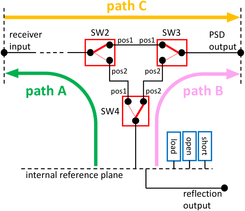
Figure 19: Diagram of the calibration network highlighting the paths that shift the internal reflection reference plane to the receiver input.

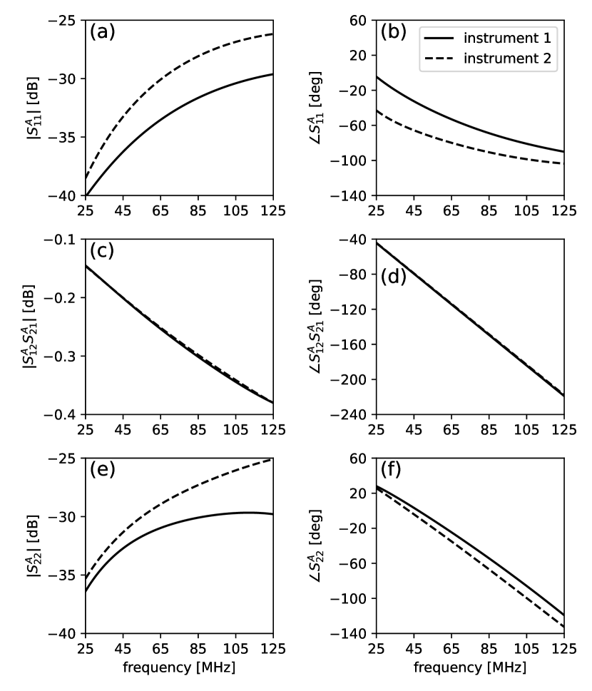
Figure 20: S-parameters of path A in the calibration network. Port $1$ corresponds to the internal reflection reference plane and port $2$ to the receiver input.

6.7 Reflection coefficient calibration

The reflection measurements described in Section 6.6 are done using the calibration network and VNA incorporated into the receiver. Our receiver calibration formalism (Section 3.2) requires these reflection measurements themselves to be calibrated at the receiver input. Furthermore, and as discussed in Monsalve et al. (2017a, b), the detection of the global $21$ cm signal requires an accuracy in reflection coefficient measurements of $\mathcal{O}(10^{-4})$. To calibrate the reflection measurements at the receiver input and with the required accuracy, MIST conducts the two-step process used by EDGES (Monsalve et al., 2017a; Bowman et al., 2018). First, a relative calibration is done using the measurements of the internal OSL standards. This step de-embeds a large fraction of the unwanted S-parameters introduced by the calibration network, the cable to the VNA, and the VNA itself. Calibrating using the internal OSL standards defines the reference plane within the calibration network. Second, the reference plane is shifted from the calibration network to the receiver input by applying S-parameter corrections determined in the lab. These corrections account for the short paths between the internal reference plane and the receiver input.

Three paths have to be accounted for and characterized. The paths, labeled A, B, and C, are shown in Figure 19. The measurements of external devices (such as the antenna) are calibrated at the receiver input by: (1) doing a relative calibration using the internal OSL standards, and (2) de-embedding the S-parameters of path A. The measurement of reflection coefficient looking into the receiver input is calibrated by: (1) doing a relative calibration using the internal OSL standards; (2) de-embedding the S-parameters of path B, which shifts the calibration plane to the PSD output; and then (3) embedding the S-parameters of path C, which shifts the calibration plane to the receiver input.

Figure 20 shows the S-parameters for path A. The parameters for paths B and C are similar and not shown for brevity. These parameters were measured in the lab and calibrated in the same way as the S-parameters of the balun (Section 5.1).

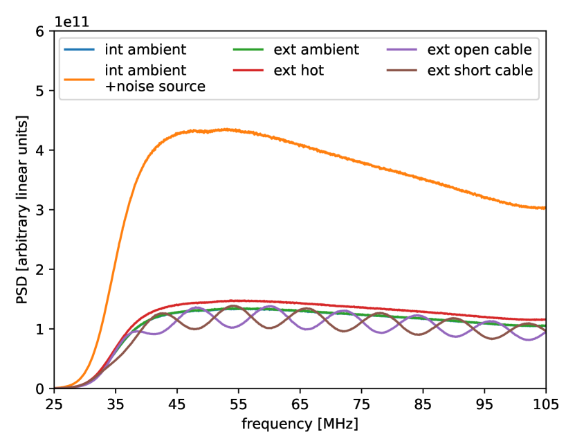
Figure 21: Sample PSDs from the internal and external calibrators measured in the lab with instrument 1. PSDs from instrument 2 are similar. Each PSD corresponds to a $10$-second integration.

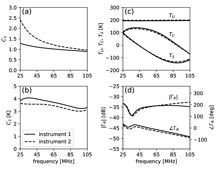
Figure 22: Absolute receiver calibration parameters and reflection coefficient looking into the receiver input for the two instruments.

6.8 Receiver calibration

We determine the five absolute receiver calibration parameters, $C_{1}$, $C_{2}$, $T_{U}$, $T_{C}$, and $T_{S}$ (see Section 3.2), from lab measurements of four external calibration devices: (1) an ambient load, (2) a hot load ($50$ $\Omega$ resistor heated up to $\approx 400$ K), (3) a $10$ m open-ended low-loss cable, and (4) the same cable after being short-circuited at its far end. For each of these devices, we measure the reflection coefficient, PSD, and physical temperature following the same procedure as for the antenna in the field (Section 6.6). Figure 21 shows sample PSDs from the internal and external calibrators measured during this process. With these measurements at hand, the five receiver parameters are computed using the iterative method of Monsalve et al. (2017a). In the computation, we use $300$ K and 2,300 K as the assumptions for the noise temperature of the internal ambient load ($T^{a}_{L}$) and ambient load plus noise source ($T^{a}_{L+NS}$), respectively. Figure 22 shows the five parameters, as well as the reflection coefficient looking into the receiver input, for the two receivers.

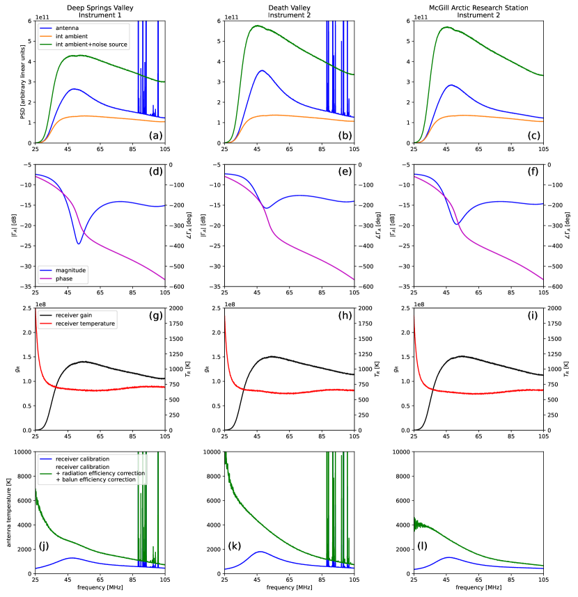
Figure 23: Sample measurements from MIST taken at the three observation sites. These measurements preliminarily show that MIST is performing as expected. The columns correspond to data from: (left) Deep Springs Valley taken with instrument $1$; (middle) Death Valley taken with instrument $2$; and (right) MARS taken with instrument $2$. (Top row) PSDs from the antenna and internal calibrators corresponding to $10$-second integrations taken at an LST=$15$ h. RFI has not been excised from the antenna measurements, which highlights the excellent radio-quiet conditions at MARS. (Second row) Antenna reflection coefficient at the balun output. (Third row) Receiver gain and temperature. (Bottom row) $41$-second antenna temperature spectra after (1) receiver calibration, and (2) receiver calibration plus radiation and balun efficiency corrections.

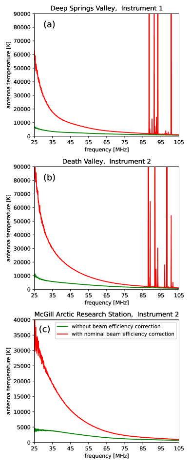
Figure 24: Sample $41$-second spectra from Deep Springs Valley, Death Valley, and MARS, before and after beam efficiency correction. RFI has not been excised from these measurements, which highlights the excellent radio-quiet conditions at MARS. In panel (c), the upper limit of the $y$ axis was reduced to 40,000 K to show the data from MARS in more detail. The beam efficiency used here corresponds to the nominal soil model (Table 2). This beam efficiency is used only as an example. In the future, we will refine the soil model based on in-situ measurements of the antenna reflection coefficient. The spectra without correction (green lines) are reproduced from Figure 23, panels (j), (k), and (l).

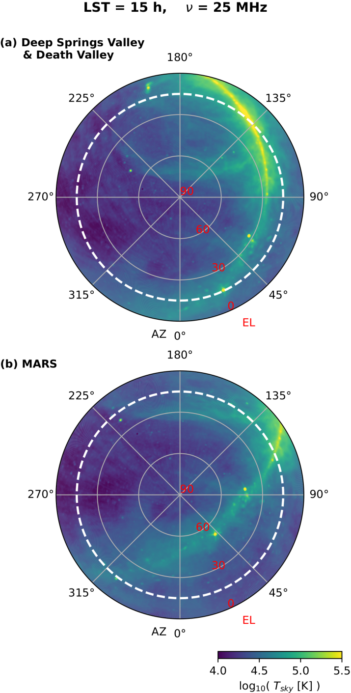
Figure 25: View of the sky at LST=$15$ h and $25$ MHz from: (a) Deep Springs Valley and Death Valley, both of which are at a latitude of $\approx 37.3^{\circ}$ N; and (b) MARS, at a latitude of $\approx 79.38^{\circ}$ N. For this figure, we used the Global Sky Model (de Oliveira-Costa et al., 2008; Price, 2016). The dashed lines represent the $-10$ dB contours of the beam directivity at $25$ MHz for the nominal soil model, shown as reference.

7 Field measurements

Between May and July 2022, we conducted sky measurements with MIST in Deep Springs Valley in California ($37.34583^{\circ}$ N, $118.02555^{\circ}$ W), Death Valley in Nevada ($37.21333^{\circ}$ N, $117.09111^{\circ}$ W), and MARS in the Canadian High Arctic ($79.37980^{\circ}$ N, $90.99885^{\circ}$ W). The Deep Springs Valley and Death Valley sites were used for observations because they offer a relatively low-RFI environment (Monsalve & Mozdzen, 2014; Anderson & Eastwood, 2016) and flat soil while remaining close to urban areas. These sites are, respectively, $\approx$20 km and $\approx$100 km east of the Owens Valley Radio Observatory (OVRO) (D’addario & Hodges, 2019). MARS is located $>$1,800 km away from cities and possesses an extremely low-RFI environment (Dyson et al., 2021).

Figures 23 and 24 show short sample measurements from the three sites. These data preliminarily indicate that MIST is performing as expected. A more in-depth discussion of instrument performance, observing sites, and analysis of the full data sets will be presented in future papers.

7.1 Power spectral densities

Each column of Figure 23 corresponds to one of the three sites. Instrument $1$ was used at Deep Springs, and instrument $2$ was used at Death Valley and MARS. The top row of the figure shows raw, unprocessed PSDs from the antenna, the internal ambient load, and the ambient load plus noise source. Each of the PSDs is a $10$-second integration. In each panel, the internal measurements belong to the same PSD cycle as the antenna measurement, which was taken around 15:00 local sidereal time (LST). The data shown from Deep Springs and Death Valley were taken at night, while those from MARS are from the continuous daytime of the Arctic summer. We have not excised RFI from these measurements.

7.2 Reflection coefficient at balun output

The second row in Figure 23 shows the calibrated reflection coefficient of the antenna at the balun output. This quantity was measured at the beginning of the same $111$-minute measurement block as the PSDs. We see that the magnitude and phase have the same general shape as those shown in Figure 13, which were obtained from electromagnetic simulations propagated through the balun S-parameters. One feature that differentiates the three sites is the magnitude dip at $\approx 50$ MHz. This dip reaches $\approx-25$, $-16$, and $-20$ dB, at Deep Springs Valley, Death Valley, and MARS, respectively. The reflection coefficient is sensitive to the soil parameters, as discussed in Sections 4.5 and 5.2. Taking advantage of this sensitivity, the soil properties at the different observing sites can be estimated by fitting electromagnetic simulations to the measured reflection. This analysis will be presented in future work.

7.3 Receiver gain and temperature

The third row in Figure 23 shows the receiver gain and temperature for the three observations. The receiver gain and temperature were computed using Equations 6 and 7, respectively, and the PSDs from the internal calibrators shown in the first row. The gain (temperature) is relatively stable across the frequency range but quickly decreases (increases) toward lower frequencies below $\approx 45$ MHz due to the two $48$ MHz high-pass filters used in the amplification chain to suppress shortwave RFI. The gain and temperature are similar between the two instruments and three observations, with differences $<10\%$.

7.4 Receiver calibration, and radiation and balun efficiency correction

The bottom row of Figure 23 shows the antenna temperature spectrum obtained from the PSD after applying: (1) receiver calibration, and (2) receiver calibration plus radiation and balun efficiency corrections. Applying the receiver calibration consists of applying to the antenna PSD the receiver gain and temperature shown in the third row of the figure following Equation 5. The receiver gain and temperature are computed using the measurements of the internal calibrators from the same PSD cycle. Because the PSD cycles have a duration of $41$ seconds (Table 3), we refer to the antenna temperature spectra as $41$-second integrations.

The antenna temperature with only receiver calibration and still affected by all the losses is significantly lower than expected from the astrophysical foreground in the northern hemisphere (Bernardi et al., 2016; Dowell et al., 2017; Dowell & Taylor, 2018; Spinelli et al., 2021). Furthermore, the antenna temperature has a peak at $\approx 45$–$50$ MHz and a decrease toward lower frequencies, departing from the power law that characterizes the foreground. This departure is mainly caused by the balun efficiency which, as Figure 14 shows, decreases quickly toward lower frequencies.

After applying the radiation and balun efficiency corrections the antenna temperature increases significantly, especially at low frequencies, and its shape becomes closer to the expected power law. Since the radiation efficiency is $>99.9\%$ (Figure 4) while the balun efficiency peaks at $\approx 45\%$ (Figure 14), the balun efficiency correction dominates the combined correction.

7.5 Beam efficiency correction

Figure 24 shows an example of the beam efficiency correction. For this example we use the nominal beam efficiency, i.e., the beam efficiency produced by the FEKO simulation that uses the nominal single-layer soil model. As Figure 8 shows, the nominal beam efficiency ranges between $11\%$ at $25$ MHz and $56\%$ at $105$ MHz. This curve is not expected to represent well the soil properties at our observation sites. Measuring soil electrical properties to inform more accurate, site-specific beam efficiency corrections is work in progress and will be discussed in future papers.

Figure 24 shows that, after beam efficiency correction, the antenna temperature from the three sites increases significantly and its shape becomes closer to the power law expectation. The sites in Deep Springs Valley and Death Valley are at a similar latitude ($\approx 37.3^{\circ}$ N). Therefore, at the same LST these sites have a similar visible sky and sky-averaged contribution to the antenna temperature. The difference seen in Figure 24 between the corrected spectra from these two sites is mainly due to different beam efficiencies in the observations resulting from different soil characteristics. The spectrum from Deep Springs Valley, in particular, still shows structure that deviates from a power law. This structure is an indication that the soil at this site departs in important ways from the nominal soil model used for the figure.

The MARS spectrum differs from the others because of the site’s contrasting soil characteristics and significantly higher latitude ($\approx 79.38^{\circ}$ N). Figure 25 shows a view of the sky at $25$ MHz and LST=$15$ h from both latitudes. The fraction of the Galactic plane that is visible from Deep Springs Valley and Death Valley is larger than from MARS.

7.6 Preliminary spectral index

As a preliminary characterization of the calibrated and efficiency corrected spectra presented in Section 7.5, here we compute their spectral index. Since the beam efficiency correction applied as an example in Section 7.5 corresponds to the nominal soil model, the accuracy of the spectral indices is not expected to be high. Furthermore, we have not removed from the data the effect produced by the frequency dependence of the beam directivity, i.e., the “beam chromaticity”. The beam chromaticity changes the spatial weighting of the sky brightness temperature as a function of frequency and, thus, can have a significant impact on the spectral index (e.g., Mozdzen et al., 2017, 2019; Spinelli et al., 2021). As discussed in Section 4.3, the beam directivity is very sensitive to the properties of the soil, highlighting again that soil characterization a critical task for MIST. We will address this aspect in future analyses.

Instead of fitting functions to the data, we take a simpler approach and compute the spectral index across our frequency range as

$$\beta=\frac{\log\left(\frac{T_{S}(105\;\mathrm{MHz})}{T_{S}(25\;\mathrm{MHz})}\right)}{\log\left(\frac{105\;\mathrm{MHz}}{25\;\mathrm{MHz}}\right)},$$ (18)

Table 4: Spectral index for the sample spectra from the three observation sites. Beam efficiency correction has been applied but assuming the nominal soil model. Beam chromaticity correction has not been applied.

Site	$T_{S}(25\leavevmode\nobreak\ \mathrm{MHz})$	$T_{S}(105\leavevmode\nobreak\ \mathrm{MHz})$	$\beta$
Deep Springs Valley	60,000 K	1,100 K	$-2.79$
Death Valley	90,000 K	1,150 K	$-3.04$
MARS	35,000 K	950 K	$-2.51$

where $T_{S}$ is the calibrated and efficiency corrected sky spectrum.

Table 4 shows the antenna temperatures and spectral index for the three sites. For Deep Springs Valley, Death Valley, and MARS, the spectral indices are $-2.79$, $-3.04$, and $-2.51$, respectively. These values are in broad agreement with previous results for the northern hemisphere (e.g., Dowell & Taylor, 2018; Spinelli et al., 2021). This agreement is a good indication for MIST, and future refinements of the beam efficiency, as well as beam chromaticity correction, should improve the results.

8 Summary and conclusions

In this paper, we have provided an overview of the two instruments built so far as part of the MIST global $21$ cm ground-based experiment. The instruments are single-antenna, single-polarization, total-power radiometers measuring the sky in the range $25$–$105$ MHz. For the $21$ cm signal, this range corresponds to redshifts $55.5>z>12.5$, which encompasses the Dark Ages and Cosmic Dawn.

Distinctive characteristics of MIST compared with the existing instruments are:

1. MIST operates above the soil but without a metal ground plane. This choice was made to avoid systematic effects from the ground plane and its interaction with the antenna. Not using a ground plane results in a higher ground loss and overall dependence of the antenna performance on the soil’s electrical characteristics. However, this choice defines an instrumental parameter space that interacts with the $21$ cm signal differently from current experiments.

2. The instruments have been designed with high portability and compactness in mind in order to conduct measurements from remote sites. Before assembly, the largest parts of the instrument are the $3$ mm thick, $1.2$ m $\times$ $0.6$ m antenna panels. The instruments are battery-powered and have a maximum power consumption of only $17$ W. The batteries and all the electronics apart from the balun are contained in a single metal receiver box located under the antenna. This compactness eliminates systematics related to cables near the antenna and is a unique aspect of MIST, contrasting with other experiments where the back-end or auxiliary electronics are kept at a secondary location.

3. The MIST observation procedure includes measurements of the antenna reflection coefficient and the reflection coefficient looking into the receiver input. These reflection measurements are done every $111$ minutes with a VNA integrated into the instrument. The antenna reflection measurements, in addition to being used for receiver calibration, will be used to precisely determine the electrical parameters of the soil. This represents another unique aspect of MIST.

4. Thanks to its portability and low power consumption, MIST has already conducted observations from Deep Springs Valley in California and Death Valley in Nevada, as well as from the McGill Arctic Research Station at a latitude of $\approx 79.38^{\circ}$ N. MARS, in particular, offers excellent radio-quiet conditions and a view of the sky that differs from, and thus complements, observations from lower latitudes by MIST and other experiments.

We quantified the performance of the MIST antenna using electromagnetic simulations and showed results for the beam directivity, radiation efficiency, beam efficiency, and reflection coefficient. Through examples, we have described how these parameters depend on the soil characteristics. As expected, the parameters are more sensitive to soil changes that occur closer to the surface, but changes below the surface are also significant and produce spectral ripples in the parameters. In a future paper (Monsalve et al., in prep.), we will discuss the impact of the MIST beam directivity on the global $21$ cm signal extraction for different soil characteristics.

We have shown sample sky measurements taken in 2022 with the two MIST instruments from Deep Springs Valley, Death Valley, and MARS. These measurements are short integrations with different levels of calibration, including a preliminary correction for beam efficiency that should improve in the future after an accurate determination of the soil electrical parameters. The measurements preliminarily show that the instruments have the expected performance in the field. We computed initial estimates for the sky spectral index and they were found in the range $\approx-2.5$ to $\approx-3$, consistent with previous measurements (Dowell & Taylor, 2018; Spinelli et al., 2021). These values will be refined after improving the beam efficiency correction and applying beam chromaticity correction. We leave for future work the detailed analysis of the data taken in 2022.

Taking advantage of MIST’s portability, we plan to carry out joint analyses leveraging observations from different latitudes over different soils to help separate the $21$ cm signal from other spectral contributions. This strategy is conceptually similar to some suggested in previous works where, for instance, data from more than one antenna, sidereal time, or Stokes polarization component, are used to improve the signal separation (Nhan et al., 2019; Tauscher et al., 2020; de Lera Acedo et al., 2022; Saxena et al., 2022; Anstey et al., 2023).