A High-Order Ultra-Weak Variational Formulation for Electromagnetic Waves Utilizing Curved Elements

Abstract

The Ultra Weak Variational Formulation (UWVF) is a special Trefftz discontinuous Galerkin method, here applied to the time-harmonic Maxwell’s equations. The method uses superpositions of plane waves to represent solutions element-wise on a finite element mesh. We focus on our parallel UWVF implementation, called ParMax, emphasizing high-order solutions in the presence of scatterers with piecewise smooth boundaries. We explain the incorporation of curved surface triangles into the UWVF, necessitating quadrature for system matrix assembly. We also show how to implement a total field and scattered field approach, together with the transmission conditions across an interface to handle resistive sheets. We note also that a wide variety of element shapes can be used, that the elements can be large compared to the wavelength of the radiation, and that a low memory version is easy to implement (although computationally costly). Our contributions are illustrated through numerical examples demonstrating the efficiency enhancement achieved by curved elements in the UWVF. The method accurately handles resistive screens, as well as perfect electric conductor and penetrable scatterers. By employing large curved elements and the low memory approach, we successfully simulated X-band frequency scattering from an aircraft. These innovations demonstrate the practicality of the UWVF for industrial applications.

1 Introduction

A Trefftz method [24] for approximating a linear partial differential equation is a numerical method using local solutions of the underlying partial differential equation as basis functions. The version we shall study here, the Ultra Weak Variational Formulation (UWVF) of Maxwell’s equations, is a Trefftz type method for approximating the solution of Maxwell’s equations on a bounded domain due to O. Cessenat and B. Després [5, 6]. The UWVF uses a finite element computational grid, classically composed of tetrahedral elements, and plane wave solutions of Maxwell’s equations on each element.

A study of this method from the point of view of symmetric hyperbolic systems was presented in [13] where the inclusion of the Perfectly Matched Layer absorbing condition [3] into the UWVF was also described. In addition, several computational heuristics relevant to our study were also presented. As a result of this work, a first parallel implementation of the UWVF called ParMax was written. This was further developed at Kuava Inc, and the University of Eastern Finland and is the basic software used in this paper. ParMax uses MPI and domain decomposition to implement parallelism.

From the point of view of theoretical convergence analysis, it was shown in [4] that the UWVF for the related Helmholtz equation is a special discontinuous Galerkin (DG) method, and using duality theory convergence estimates could be proved. A more general DG approach, again for the Helmholtz equation, is taken in [7]. Based on these studies, and following the proof of explicit stability bounds for the interior impedance boundary value problem for Maxwell’s equations in [10], convergence of Trefftz DG methods (in particular the UWVF) for Maxwell’s equations under rather strict geometric assumptions was proved in [11]. A key point in this analysis is that it is not necessary to use tetrahedral elements, but a wide class of element shapes are theoretically covered and we shall return to this point in Section 3.

A restriction on the use of the UWVF is that the relative electric permittivity denote $\epsilon_{\mathrm{r}}$ and relative magnetic permeability $\mu_{\mathrm{r}}$ must be piecewise constant (constant on each tetrahedron in the mesh). This assumption could perhaps be weakened using generalised plane waves [14] or embedded Trefftz techniques [17] but these have not yet been extended to Maxwell’s equations (the latter technique has been demonstrated in the open source package [23]). The restriction of piecewise constant media is relaxed if a Perfectly Matched Layer (PML) is used. There $\epsilon_{\mathrm{r}}$ and $\mu_{\mathrm{r}}$ are spatially varying tensors [13].

The main issue facing the UWVF is that the condition number of the global system rises rapidly as the number of plane wave directions increases. This in turn causes the iterative solution of the linear system to slow down. We adopt the approach of [13] choosing the number of plane wave directions on a given element on the basis of its geometric size (in wavelengths) to control ill-conditioning.

We use the same stabilised BiConjugate Gradient (BICGstab) scheme as in [13] for solving the global linear system resulting from the UWVF. Interesting new results on preconditioned iterative schemes can be found in [20]. These results are based on the use of a structured hexahedral grid, whereas we focus on unstructured grids in this paper.

Within the UWVF scheme used here there is considerable scope for different choices of basis functions provided they form a complete family of solutions of Maxwell’s equations. For example, plane wave basis functions (as used here), vector wave functions or the method of fundamental solutions (MFS) are discussed in [2]. In the interesting case of MFS, [8] gives an application to wave guides. to the method. Our choice of plane waves in ParMax follows [5] and has the advantage that necessary integrals of products of basis functions can be performed in closed form on flat triangular faces in the mesh (the majority of faces). This greatly speeds up the assembly of matrices compared to quadrature that is needed for other choices of basis functions.

In this paper, $i=\sqrt{-1}$ and we use the convention that the time variation of the fields and sources is proportional to $\exp(-i\omega t)$ where $\omega$ is the angular frequency of the radiation, and $t$ is time. All results are then reported in the frequency domain. Bold face quantities are vector valued. The coefficients $\epsilon_{0}$ and $\mu_{0}$ are the permittivity and permeability of free space respectively. The wave number $\kappa$ of the radiation is given by $\kappa=\omega\sqrt{\epsilon_{0}\mu_{0}}$.

To further fix notation and context, we now define the Maxwell system under consideration in this paper. Let $\Omega$ denote a Lipschitz bounded computational domain having unit outward normal $\bm{\nu}$ and boundary $\Gamma:=\partial\Omega$. For a smooth enough vector field $\mathbf{v}$, we define the tangential component $\mathbf{v}_{T}$ on $\Gamma$ by $\mathbf{v}_{T}=(\bm{\nu}\times\mathbf{v})\times\bm{\nu}$. Then, given the wave number $\kappa>0$, a tangential boundary vector field $\mathbf{g}$, piecewise constant functions $\epsilon_{\mathrm{r}}$ and $\mu_{\mathrm{r}}$, and a parameter $Q\in\mathbb{C}$ with $|Q|\leq 1$ we seek the complex valued vector electric field $\mathbf{E}$ that satisfies

$$\operatorname{curl}\mu_{\mathrm{r}}^{-1}\operatorname{curl}\mathbf{E}-\kappa^{2}\epsilon_{\mathrm{r}}\mathbf{E} =0\mbox{ in }\Omega,$$ (1a)

$$\bm{\nu}\times\mu_{\mathrm{r}}^{-1}\operatorname{curl}\mathbf{E}+\frac{i\kappa}{Z}\mathbf{E}_{T} =Q\left(-\bm{\nu}\times\mu_{\mathrm{r}}^{-1}\operatorname{curl}\mathbf{E}+\frac{i\kappa}{Z}\mathbf{E}_{T}\right)+\mathbf{g}\mbox{ on }\Gamma.$$ (1b)

Here $Z$ is the surface impedance (a positive real parameter). The boundary condition (1b) is of impedance type and is well suited to the UWVF. When $Q=-1$ it gives a rotated version of the Perfectly Electrically Conducting (PEC) boundary condition for the scatterered wave

$$\mathbf{E}_{T}=\frac{Z}{2i\kappa}\mathbf{g},$$

where we take $g=-2i\kappa\mathbf{E}^{i}_{T}/Z$ and $\mathbf{E}^{i}$ is the incident wave. When $Q=0$ it corresponds to an outgoing condition that can be used as a low order radiation condition, while for $Q=1$ we have a symmetry boundary condition.

This paper presents several novel extensions of the basic UWVF that are of considerable utility in practical applications. In particular:

• The original UWVF uses a tetrahedral grid, however the error estimates in [11] hold for more general element types. Besides tetrahedral elements, we have implemented hexahedral and wedge elements. In this paper, hexahedral elements are only used in the PML region.

• Very often curved surfaces appear in applications, and we have implemented a mapping technique to approximate smooth curved surfaces. This allows us to use larger elements near a curved boundary. We shall show, using numerical experiments, that this improves the efficiency of the software by decreasing the overall time to compute a solution. Note that we only need to map faces in the mesh which simplifies the implementation, but we have to use quadrature to evaluate integrals on curved faces.

• We show how to implement resistive sheet transmission conditions across thin interfaces. Related to this we have also implemented a combined total field and scattered field formulation to allow the solution of problems involving penetrable media.

• We point out that a low memory version can be used to solve very large problems by avoiding the storage of the most memory intensive matrix in the algorithm.

• We provide numerical results to justify the utility of the above innovations.

The paper proceeds as follows. In Section 2 we start with a brief derivation of the basic UWVF and describe the plane wave based UWVF. Then in Section 3 we describe the five contributions of this paper. We start with comments on new geometric element types and a brief discussion of implementing an algorithm for using scattered or total fields in different subdomains in the context of scattering from a penetrable object. Then we move to discuss resistive sheets, curved elements and quadrature, and finally a lower memory version of the method. Section  4 is devoted to numerical examples illustrating the UWVF and the previously mentioned modifications. In Section 4.1 we start with two examples of scattering from a PEC scatterer. The first PEC example is scattering from a sphere for which the Mie series gives an accurate solution for comparison (c.f. [19]). This example demonstrates the benefits of curved elements and different element types, as well as the use of very coarse meshes (compared to those used by finite element methods). The second example is X-band scattering from an aircraft model. Here again we use curved elements, but in addition use the low-memory version of the software. In Section 4.2 we consider two examples involving a resistive sheet. The first is a classical example having an exact analytical solution, and the second is a resistive screen surrounding a sphere. Next, in Section 4.3, we consider heterogeneous or penetrable scatterers. The first example is a dielectric sphere where we use the scattered/near field formulation and compare to the Mie series solution. The second example is scattering from a plasma. In Section 5 we present our conclusions. Finally in Appendix A we give an update to the basis selection rule used previously in [13] for the new element types. Then, in Appendix B, we present a comparison of ParMax with the edge finite element method for scattering from a dielectric sphere.

2 Derivation and properties of the basic UWVF

In this section we provide a sketch of the derivation of the UWVF sufficient to allow us to present the new features of this paper in the following section. For full details see [5, 13].

2.1 A brief derivation of the UWVF

The version of the UWVF presented here is equivalent to that used in ParMax (from [5]) but with simplified notation. Consider a mesh of $\Omega$ of elements of maximum diameter $h$ denoted by ${\cal T}_{h}$. An element $K\in{\cal T}_{h}$ in this mesh is a curvilinear polyhedron (curvilinear tetrahedron, wedge, or hexahedron) with boundary denoted by $\partial K$ and unit outward normal $\bm{\nu}^{K}$. We now extend the parameter $Z$ to a real piecewise positive constant defined on all faces in the grid. Following [5], we choose $Z$ as follows. Let

$$\hat{\epsilon}=\left\{\begin{array}[]{rl}|\sqrt{\epsilon_{\mathrm{r}}|_{K}\,\epsilon_{\mathrm{r}}|_{K^{\prime}}}|&\mbox{on }K\cap K^{\prime}\mbox{ for }K,K^{\prime}\in{\cal T}_{h}\\ |{\epsilon_{\mathrm{r}}}|&\mbox{on boundary faces}\end{array}\right.$$

where $|_{K}$ denotes the restriction to $K$. The edge function $\hat{\mu}$ is defined in the same way. Then $Z=\sqrt{\hat{\mu}}/\sqrt{\hat{\epsilon}}$.

Suppose $\bm{\xi}$ is a smooth solution of the adjoint Maxwell equation in $K$:

$$\operatorname{curl}\overline{\mu_{\mathrm{r}}}^{-1}\operatorname{curl}\bm{\xi}-\kappa^{2}\overline{\epsilon_{\mathrm{r}}}\bm{\xi}=0.$$ (2)

Then taking the dot product of (1a) with $\bm{\xi}$ (including complex conjugation) and integrating by parts twice provides the following fundamental relation between the electric and magnetic fluxes on $\partial K$:

$$\int_{\partial K}{\bm{\nu}^{K}\times\mu_{\mathrm{r}}^{-1}\nabla\times\mathbf{E}}\cdot\overline{\bm{\xi}}_{T}+{\bm{\nu}^{K}\times\mathbf{E}}\cdot(\overline{\overline{\mu_{\mathrm{r}}}^{-1}\nabla\times\bm{\xi}})_{T}\,dA=0.$$ (3)

Using the above fundamental identity, we can then prove equality (4) by expanding both sides of (4) and using (3). Equality (4) gives the conclusion of the “isometry lemma” (c.f. [5]).

$$\int_{\partial K}Z\left(-\bm{\nu}^{K}\times\mu_{\mathrm{r}}^{-1}\nabla\times\mathbf{E}+\frac{i\kappa{}}{Z}\mathbf{E}_{T}\right)\cdot\left(-\overline{\bm{\nu}^{K}\times{\overline{}}\mu_{\mathrm{r}}^{-1}\nabla\times\bm{\xi}+\frac{i\kappa{}}{Z}\bm{\xi}_{T}}\right)\,dA.$$ (4)

$$= \int_{\partial K}Z\left(\bm{\nu}^{K}\times\mu_{\mathrm{r}}^{-1}\nabla\times\mathbf{E}+\frac{i\kappa{}}{Z}\mathbf{E}_{T}\right)\cdot\left(\overline{\bm{\nu}^{K}\times{}\mu_{\mathrm{r}}^{-1}\nabla\times\bm{\xi}+\frac{i\kappa{}}{Z}\bm{\xi}_{T}}\right)\,dA$$

To simplify the presentation, we define rescaled versions of the unknowns in [5] as follows:

$$\bm{\chi}_{K} = -\bm{\nu}^{K}\times\mu_{\mathrm{r}}^{-1}\nabla\times\mathbf{E}|_{K}+\frac{i\kappa{}}{Z}(\mathbf{E}|_{K})_{T}$$ (5)

$${\cal Y}_{K} = -\bm{\nu}^{K}\times\mu_{\mathrm{r}}^{-1}\nabla\times\bm{\xi}|_{K}+\frac{i\kappa{}}{Z}(\bm{\xi}|_{K})_{T}.$$ (6)

The next step is to rewrite (4) using the above quantities. In doing so we will use the function space of surface vectors $\mathbf{L}_{T}^{2}(\partial K):=\{\mathbf{u}\in\mathbf{L}^{2}(\partial K)\;|\;\mathbf{u}\cdot\bm{\nu}^{K}=0\}$. Recalling that $\bm{\xi}|_{K}$ satisfies the adjoint Maxwell system in $K$ we can define $\mathbf{F}_{K}:\mathbf{L}_{T}^{2}(\partial K)\to\mathbf{L}_{T}^{2}(\partial K)$ by setting

$$\mathbf{F}_{K}{\cal Y}_{K}=\bm{\nu}^{K}\times\mu_{\mathrm{r}}^{-1}\nabla\times\bm{\xi}|_{K}+i\kappa{}Z(\bm{\xi}|_{K})_{T}.$$

Now suppose elements $K$ and $K^{\prime}$ meet at a face in the mesh. On that face $\bm{\nu}^{K}=-\bm{\nu}^{K^{\prime}}$. Also we have transmission condition requiring continuity of $\mathbf{E}_{T}$ and $(\mu_{\mathrm{r}}^{-1}\nabla\times\mathbf{E})_{T}$ across the face so

$$\bm{\nu}^{K}\times\mu_{\mathrm{r}}^{-1}\nabla\times\mathbf{E}|_{K}+i\omega{}Z(\mathbf{E}|_{K})_{T}=\bm{\chi}_{K^{\prime}}.$$ (7)

For a boundary face we can use the boundary condition (1b) to replace the corresponding term on that face in terms of $\bm{\chi}_{K}$ and $\mathbf{g}$. Using the above results, we may rewrite (4) for every element $K$. We conclude that for $\bm{\chi}_{K}\in\mathbf{L}_{T}^{2}(\partial K)$ the following equation holds

$$\int_{\partial K}Z\,\bm{\chi}_{K}\cdot{\cal Y}_{K}\,dA= \sum_{K^{\prime}\not=K}\int_{\partial K\cap\partial K^{\prime}}Z\,\bm{\chi}_{K^{\prime}}\cdot\mathbf{F}_{K}{\cal Y}_{K}\,dA$$

$$+\int_{\partial K\cap\partial K^{\prime}} Z\left[Q\bm{\chi}_{K}+\mathbf{g}\right]\cdot\mathbf{F}_{K}{\cal Y}_{K}\,dA,$$ (8)

for any ${\cal Y}_{K}\in\mathbf{L}^{2}_{T}(\partial K)$. This equation should hold for every $K\in{\cal T}_{h}$, and gives the UWVF for Maxwell’s equations before discretization. Cessenat [5] proves the uniqueness of the UWVF solution, and existence follows because (1a)-(1b) is well posed.

2.2 The plane wave UWVF (PW-UWVF)

Now that we have the variational formulation (8) we can discretize it by using a subspace of $\mathbf{L}^{2}_{T}(\partial K)$ on each element. It is important for efficiency that $\mathbf{F}_{K}$ be easy to compute and this is where the plane wave basis is useful [5]. On each element $K$ we choose independent directions $\{\mathbf{d}_{K,j}\}_{j=1}^{p_{K}}$, $\|\mathbf{d}_{K,j}\|=1$, using the first $p_{K}$ Hammersley points [9] on the unit sphere. Then we choose $\bm{\xi}|_{K}$ to be a linear combination of the $p_{K}$ plane wave solutions of the adjoint problem

$$\bm{\xi}_{K,\ell,m}=\mathbf{A}_{K,\ell,m}\exp\left(i\kappa\sqrt{\overline{\epsilon_{\mathrm{r}}|_{K}}\overline{\mu_{\mathrm{r}}|_{K}}}\mathbf{d}_{K,\ell}\cdot(\mathbf{x}-\mathbf{x}_{K,0})\right)$$

for $1\leq\ell\leq P_{K},$ $1\leq m\leq 2,$ and $K\in{\cal T}_{h}$. Here $\mathbf{x}_{K,0}$ is the centroid of the element and the polarizations $\mathbf{A}_{K,\ell,m}$ are chosen to be unit vectors such that $\mathbf{d}_{K,\ell}\cdot\mathbf{A}_{K,\ell,m}=0$, $m=1,2$ and $\mathbf{A}_{K,\ell,1}\cdot\mathbf{A}_{K,\ell,2}=0$. Now we can define a discrete subspace $\mathbf{W}_{K,h}\subset\mathbf{L}_{T}^{2}(\partial K)$ by first defining

$$\mathbf{W}_{K,h,p_{K}}={\rm span}\{-\bm{\nu}^{K}\times\mu_{\mathrm{r}}^{-1}\nabla\times\bm{\xi}_{K,\ell,m}$$

$$\qquad+(i\kappa/Z)(\bm{\xi}_{K,\ell,m})_{T},\;m=1,2,\;1\leq\ell\leq p_{K}\}.$$

Then $\mathbf{W}_{h,\mathbf{p}}=\Pi_{K\in{\cal T}_{h}}\mathbf{W}_{K,h,p_{K}}$ where $\mathbf{p}$ denotes the vector of number of directions on each element.

The dimension of $W_{h,\mathbf{p}}$ is $N_{\mathrm{DoF}}=2\sum_{K\in{\cal T}_{h}}p_{K}$. In our work, $p_{K}$ is chosen according to the heuristic in [13] (see Appendix A for updates to this formula for larger numbers of directions and new element types). Then $\mathbf{F}_{K}$ is easy to compute using the definition of the basis functions. The discrete PW-UWVF uses trial and test functions from $\mathbf{W}_{h,\mathbf{p}}$ in place of $\mathbf{W}$ in (8).

In our implementation, we use domain decomposition by subdividing the mesh according to Metis [16] where $p_{K}$ is used to estimate the work on each element. The elements are sorted using reverse Cuthill-McKee to minimise bandwidth. Then, enumerating the degrees of freedom element by element, the matrices and vectors corresponding to the terms in (8) can be computed. The left hand side of (8) gives rise to an $N_{\mathrm{DoF}}\times N_{\mathrm{DoF}}$ block diagonal Hermitian positive-definite matrix $D$, while the remaining sesquilinear forms on the right hand side of (8) give rise to a general sparse complex matrix $C$. The data term involving $\mathbf{g}$ gives rise to a corresponding vector $\vec{\mathbf{b}}$. Denoting the vector of unknown degrees of freedom by $\vec{\bm{\chi}}$, we solve the global matrix equation

$$(I-D^{-1}C)\vec{\bm{\chi}}=D^{-1}\vec{\mathbf{b}}$$ (9)

using BICGstab where $D^{-1}$ can be calculated rapidly element by element. Once $\vec{\bm{\chi}}$ is known, the solution on each element can be reconstructed for post processing. For unbounded scattering problems, we use either the low order absorbing condition ($Q=0$) on the outer boundary or a PML as in [13]. For a scattering problem the far field pattern can the be calculated using an auxiliary surface containing all the scatterers in its interior in the usual way [5].

3 Towards industrial scale software

In this section we discuss the extensions to the basic UWVF in this paper.

3.1 New element types

In [11] error estimates are proved for general elements that have Lipschitz boundaries, are shape regular in the sense of that paper, and are star-shaped with respect to a ball centred at a point in the element. This allows a wide variety of elements. We have implemented curvilinear tetrahedral, wedge, and hexahedral elements. In ParMax we represent the boundary of each element as a union of possibly curvilinear triangles. The assembly phase is quickest if the triangles are planar since then quadrature can be avoided.

For this paper, we rely on COMSOL Multiphysics to generate the meshes. An example of a grid using tetrahedral, wedge, and hexahedral elements is shown in Fig. 3. Here we use wedge and hexahedral elements in the PML, and tetrahedral elements elsewhere.

3.2 Scattered/total field formulation

The numerical results we shall present are all of scattering type. The total field $\mathbf{E}$ is composed of an unknown scattered field $\mathbf{E}^{s}$ and a given incident field $\mathbf{E}^{i}$ so $\mathbf{E}=\mathbf{E}^{s}+\mathbf{E}^{i}$. We will use plane wave incident fields (but point sources or other incident fields can be used) so

$$\mathbf{E}^{i}(\mathbf{x})=\mathbf{p}\exp(i\kappa\mathbf{d}\cdot\mathbf{x}),$$ (10)

where $\mathbf{d}\in\mathbb{R}^{3}$ is the direction of propagation and $\|\mathbf{d}\|=1$. The vector polarisation $\mathbf{p}\in\mathbb{C}^{3}$ is non-zero and satisfies $\mathbf{d}\cdot\mathbf{p}=0$.

To allow the use of a PML or other absorbing boundary condition, we need to compute using the scatterered field in the PML. But inside a penetrable scatterer we need to compute with the total field so that there are no current sources in the scatterer. This is standard for finite element methods, but not usual for the UWVF so we outline the process here. Suppose $\Omega$ is partitioned into two subdomains denoted $\Omega_{-}$ and $\Omega_{+}$ such that the PML (or a neighbourhood of the absorbing boundary if one is used) is contained in $\Omega_{+}$ where the scattered field is used and where $\epsilon_{\mathrm{r}}=\mu_{\mathrm{r}}=1$. The scatterer is contained in $\Omega_{-}$ where possible $\epsilon_{\mathrm{r}}$ or $\mu_{\mathrm{r}}$ are no longer unity and the total field is used. Let $\Sigma$ denote the boundary between $\Omega_{-}$ and $\Omega_{+}$ and assume that $\Sigma$ is contained in the interior of $\Omega$ and is exactly covered by faces of the mesh. Then suppose that elements $K_{-}\subset\Omega_{-}$ and $K_{+}\subset\Omega_{+}$ meet at a face $F\subset\Sigma$.

Consider first $K_{-}$. Reviewing the derivation of the UWVF outlined in Section 2.2 we see that we must rewrite the term in $\mathbf{E}$ on the right hand side of equation (4) in terms of $\bm{\chi}_{K_{-}}$ and $\bm{\chi}_{K_{+}}$. In particular using the facts that $\bm{\nu}_{K_{-}}=-\bm{\nu}_{K_{+}}$ and that on $K_{+}$ the scattered field $\mathbf{E}^{s}$ is be approximated, so that in (5) $\mathbf{E}|_{K^{+}}$ is replaced by $(\mathbf{E}^{s}+\mathbf{E}^{i})|_{K^{+}}$, we obtain

$$\left(\bm{\nu}^{K_{-}}\times\mu_{\mathrm{r}}^{-1}\nabla\times\mathbf{E}|_{K_{-}}+\frac{i\kappa{}}{Z}\mathbf{E}|_{K_{-},T}\right) = -\bm{\nu}^{K_{+}}\times\mu_{\mathrm{r}}^{-1}\nabla\times(\mathbf{E}^{s}+\mathbf{E}^{i})|_{K_{+}}$$

$$+\frac{i\kappa{}}{Z}(\mathbf{E}^{s}+\mathbf{E}^{i})|_{K_{+},T}=\bm{\chi}_{K_{+}}+\mathbf{g}_{K_{-},F}.$$

Here we have also used the transmission condition that the tangential components of $\mathbf{E}$ and $\mu_{\mathrm{r}}^{-1}\operatorname{curl}\mathbf{E}$ are continuous across $\Sigma$. In this equation, the source function on $F$ associated with $K_{-}$ is

$$\mathbf{g}_{K_{-},F}=\left(\bm{\nu}^{K_{-}}\times\mu_{\mathrm{r}}^{-1}\nabla\times\mathbf{E}^{i}|_{F}+\frac{i\kappa{}}{Z}\mathbf{E}^{i}|_{F,T}\right).$$

Carrying out the same procedure on $K_{+}$ remembering this element supports the scattered field gives another equation and source function $\mathbf{g}_{K_{+},F}$ again relating $\mathbf{E}$ and $\mathbf{E}^{s}$. Thus a combined scattered and total field algorithm can be implemented by allowing for a source function $\mathbf{g}$ on the internal surfaces.

3.3 Resistive sheet

A similar procedure to that used to implement the scattered/total field UWVF can be used to derive appropriate modifications to include resistive [15] or conductive sheets [22]. We only consider the resistive sheet. Suppose now that a surface $\Sigma_{r}\subset\Omega$ is a resistive sheet, and that $\bm{\nu}_{r}$ denotes a continuous normal to the sheet. This surface may be open or closed and could intersect the boundary. We just assume that it is the union of a subset of the faces (possibly curvilinear) in the mesh.

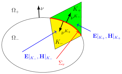
Figure 1: Geometry and notation for the resistive sheet calculation. The normal $\nu$ is outward to $\Omega_{-}$.

Suppose $K_{+}$ and $K_{-}$ are two elements that meet at a face $F_{r}\subset\Sigma_{r}$ such that $\bm{\nu}_{r}$ points into $K_{+}$. The geometry is shown in Fig. 1.

The resistive sheet approximation requires us to implement the following transmission conditions across $\Sigma_{r}$

$$\bm{\nu}_{r}\times(\mu_{\mathrm{r}}^{-1}\operatorname{curl}\mathbf{E}|_{K_{+}}-\mu_{\mathrm{r}}^{-1}\operatorname{curl}\mathbf{E}|_{K_{-}}) = i\kappa\sigma d(\bm{\nu}_{r}\times\mathbf{E}_{K_{+}})\times\bm{\nu}_{r},$$ (11)

$$(\bm{\nu}_{r}\times\mathbf{E}|_{K_{+}})\times\bm{\nu}_{r} = (\bm{\nu}_{r}\times\mathbf{E}_{K_{-}})\times\bm{\nu}_{r},$$ (12)

where $\sigma$ is the conductivity of the material in the layer and $d$ is the thickness. Alternatively the resistivity of the sheet is given by

$$R=(\sigma d)^{-1}=-\frac{Z_{0}}{i(\epsilon_{\mathrm{r}}-1)\kappa_{0}d}$$

with $\epsilon_{\mathrm{r}}=1+i\sigma/(\epsilon_{0}\omega)$, $Z_{0}=\sqrt{\mu_{0}/\epsilon_{0}}$ is the impedance of free space and $\kappa_{0}=\omega\sqrt{\mu_{0}\epsilon_{0}}$ is the wave-number. We now set $\eta=\sigma d$.

As for the scattered/total field version of UWVF we must write the term in $\mathbf{E}$ on the right hand side of (4) using the variables $\bm{\chi}|_{K_{+}}$ and $\bm{\chi}|_{K_{-}}$ on either side of $F_{r}$.

Adding $\bm{\chi}|_{K_{+}}$ to $\bm{\chi}|_{K_{-}}$, using the resistive sheet transmission conditions and noting that $\bm{\nu}^{K_{-}}=\bm{\nu}_{r}=-\bm{\nu}^{K_{+}}$ gives

$$\bm{\chi}_{K_{-}}+\bm{\chi}_{K_{+}}=i\kappa\left(\frac{2}{Z}\mathbf{E}_{K_{+},T}+\eta\mathbf{E}_{K_{+},T}\right)$$

so

$$\mathbf{E}|_{K_{+},T}=\mathbf{E}|_{K_{-},T}=\frac{\bm{\chi}_{K_{-}}+\bm{\chi}_{K_{+}}}{2i\kappa/Z+i\kappa\eta}.$$ (13)

Now we rewrite the term in $\mathbf{E}$ on the right hand side of (4) using the UWVF functions. Using Equation (13) we have

$$\bm{\nu}^{K_{-}}\times\mu_{\mathrm{r}}^{-1}\nabla\times\mathbf{E}|_{K_{-}}+\frac{i\kappa{}}{Z}\mathbf{E}|_{K_{-},T}=\bm{\nu}^{K_{-}}\times\mu_{\mathrm{r}}^{-1}\nabla\times\mathbf{E}|_{K_{-}}+\frac{1}{Z}\frac{\bm{\chi}_{K_{-}}+\bm{\chi}_{K_{+}}}{2/Z+\eta}.$$ (14)

But, using (11), we have

$$\bm{\nu}^{K_{-}}\times\mu_{\mathrm{r}}^{-1}\nabla\times\mathbf{E}|_{K_{-}}=-\bm{\nu}^{K_{+}}\times\mu_{\mathrm{r}}^{-1}\nabla\times\mathbf{E}|_{K_{+}}-i\kappa\eta\mathbf{E}_{K_{+},T}.$$

Then, using the above equality in (14) together with (13) again we have

$$\bm{\nu}^{K_{-}}\times\mu_{\mathrm{r}}^{-1}\nabla\times\mathbf{E}|_{K_{-}}+\frac{i\kappa{}}{Z}\mathbf{E}|_{K_{-},T} = -\bm{\nu}^{K_{+}}\times\mu_{\mathrm{r}}^{-1}\nabla\times\mathbf{E}|_{K_{+}}-i\kappa\eta\mathbf{E}_{K_{+},T}+\frac{1}{Z}\frac{\bm{\chi}_{K_{-}}+\bm{\chi}_{K_{+}}}{2/Z+\eta}$$

$$= \left(\bm{\chi}_{K_{+}}-\frac{\eta}{2/Z+\eta}(\bm{\chi}_{K_{-}}+\bm{\chi}_{K_{+}})\right).$$

The new term introduces a new diagonal block into the matrix $C$ (defined before (9)) and a perturbation to the off diagonal blocks coupling fields on $K_{+}$ and $K_{-}$.

In the current ParMax implementation, $\eta$ is assumed constant on each mesh face of the resistive sheet and may be complex.

3.4 Curved elements and quadrature

We take a straightforward approach to approximating curved boundaries and quadrature. All the elements in ParMax have faces that are unions of possibly curvilinear triangles. Suppose a curvilinear face $F$ in the mesh is such that either an edge of $F$, or $F$ itself are entirely contained in a smooth curvilinear subset of the boundary $\Gamma$. We approximate $F$ by a mapping from a reference element $\hat{F}$ (with vertices $\widehat{\mathbf{a}}_{1}=(0,0)$, $\widehat{\mathbf{a}}_{2}=(0,1)$, and $\widehat{\mathbf{a}}_{3}=(1,0)$) in the $(s,t)$ plane to an approximation of $F$ using a degree $\ell$ polynomial map $\mathbf{F}_{F}:\hat{F}\to F$.

In the important case of a quadratic map ($\ell=2$) we choose $\mathbf{a}_{i}$, $i=1,2,3$ to be the vertices of $K$ and take the remaining interpolation points by choosing $\mathbf{a}_{i,j}$ to be a point on the smooth boundary approximately half way between $\mathbf{a}_{i}$ and $\mathbf{a}_{j}$ (mapped from $\widehat{\mathbf{a}}_{i,j}=(\widehat{\mathbf{a}}_{i}+\widehat{\mathbf{a}}_{j})/2$; see Fig. 2). We use the following nodal basis

$$\hat{\phi}_{1}(s,t) = (1-s-t)(1-2s-2t)$$

$$\hat{\phi}_{2}(s,t) = s(2s-1)$$

$$\hat{\phi}_{3}(s,t) = t(2t-1)$$

$$\hat{\phi}_{1,2}(s,t) = 4s(1-s-t)$$

$$\hat{\phi}_{2,3}(s,t) = 4st$$

$$\hat{\phi}_{1,3}(s,t) = 4t(1-s-t)$$

and define $\mathbf{F}_{F}$ by

$$\mathbf{F}_{F}(s,t)=\sum_{i=1}^{3}\mathbf{a}_{i}\hat{\phi}_{i}(s,t)+\sum_{i=1}^{2}\sum_{j=i+1}^{3}\mathbf{a}_{i,j}\hat{\phi}_{i,j}(s,t).$$ (15)

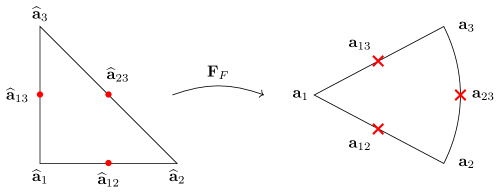
Figure 2: Sketch of mapping from the reference face to the face of an element in the volume mesh. Here we sketch a quadratic map requiring that the midpoint of each edge in the curvilinear face be given.

We use $\mathbf{F}_{F}(\hat{F})\approx F$ for computing the UWVF matrices. Thus we need to evaluate integrals over each face $\mathbf{F}_{F}(\hat{F})$. Using the reference element, for a smooth function $g$ defined in a neighbourhood of $F$

$$\int_{F}g({\bf y})dS({\mathbf{y}})\approx\int_{\mathbf{F}_{F}(\hat{F})}g({\bf y})dS({\mathbf{y}})$$

$$= \int_{\hat{F}}g(\mathbf{F}_{F}(s,t))\left\|\frac{\partial{\mathbf{F}_{F}}}{\partial s}(s,t)\times\frac{\partial{\mathbf{F}_{F}}}{\partial t}(s,t)\right\|\,ds\,dt.$$

It now suffices to define quadrature on the reference element via the Duffy transform. Suppose $G(s,t)$ is a smooth function on $\hat{F}$ (in particular the integrand above) then setting $t=(1-s)\xi$ we can map to the unit square:

$$\int_{\hat{F}}G\,d\hat{A} = \int_{0}^{1}\int_{0}^{1-s}G(s,t)\,dt\,ds$$

$$= \int_{0}^{1}(1-s)\int_{0}^{1}G(s,(1-s)\xi)\,d\xi\,ds.$$

Let $(w^{g}_{i},t_{i}^{g})$, $1\leq i\leq N$, denote the $N$-point Gauss-Legendre rule weights and nodes on $(0,1)$. Then for each $s$

$$\int_{0}^{1}G(s,(1-s)\xi)\,d\xi\approx\sum_{i=1}^{N}w_{i}^{g}G(s,(1-s)t_{i}^{g}).$$

Next, using $N$ point Jacobi quadrature weights and nodes on $(0,1)$ denoted $(w_{j}^{J},x_{j}^{J})$, we obtain finally

$$\int_{\hat{F}}G\,dA\approx\sum_{i=1}^{N}\sum_{j=1}^{N}w_{j}^{J}w_{i}^{g}f(x_{j}^{J},t_{i}^{g}(1-x_{j}^{J})).$$

Note that the quadrature has positive weights.

3.5 A low memory version

A simple low memory version of ParMax is easily available because we use BICGstab to solve the linear system. We compute $D$ as usual (it is block diagonal), and the vector $\vec{\mathbf{b}}$ but do not compute the elements of $C$ in (9). Then, as required by BICGstab, to compute $D^{-1}C\vec{\mathbf{x}}$ for some vector $\vec{\mathbf{x}}$ we compute the blocks of $C$ element by element and accumulate $C\vec{\mathbf{x}}$ element by element. Then $D^{-1}$ is computed element by element using precomputed LU decompositions. Obviously computing the entries of $C$ repeatedly greatly increases CPU time but this allows us to compute solutions to problem that would otherwise require very large memory to store $C$. For example, the solution of a scattering problem for a full aircraft at X-band frequencies is shown in Section 4.1.2.

4 Numerical examples

All results were generated using the computer clusters Puhti and Mahti at the CSC – IT Center for Science Ltd, Finland. Detailed descriptions of these supercomputers can be found from the CSC’s website [1]. Computational grids used in this work were prepared using COMSOL Multiphysics on a personal computer. In addition, the geometry model for aircraft used in Section 4.1.2 is adapted from the COMSOL’s application Simulating Antenna Crosstalk on an Airplane’s Fuselage.

For all numerical experiments, the incident electric field is a plane wave propagating in the direction of the positive $x$-axis polarised in the $y$-direction where the field is given by (10).

4.1 Scattering from PEC objects

In both PEC examples, we compute the scattered field and the incident field is used as a source via the PEC condition on the surface of the scatterer.

4.1.1 A sphere

This experiment is intended to demonstrate the advantages of multiple element types, and a cuvilinear approximation to a smooth curved boundary (the surface of the sphere). In particular, we study scattering from a PEC sphere placed in vacuum, $\epsilon_{\mathrm{r}}=\mu_{\mathrm{r}}=1$, where the frequency of the incident field is $f=2$ GHz (wavelength in air: $\lambda_{0}=0.19946$ m). The scatterer is a PEC sphere with radius of 1 meter or approximately $5\lambda_{0}$.

In order to demonstrate the use of several types of large elements and curvilinear grids, we use an unusually large computational domain. In particular, the sphere is placed with its origin at the center of a cube shaped computational domain $[-1-15\lambda_{0},1+15\lambda_{0}]^{3}$.

An absorbing boundary condition, (1b) with $Q=0$, is used on the exterior surface geometry. In addition, a PML with thickness of $5\lambda_{0}$, and constant absorption parameter $\sigma_{0}=1$ is used within each side of the cube.

Two computational grids with different geometric approximations are used (see Fig. 3). For the first grid (mesh 1), we set the requested element size on the PEC sphere to be $h_{\mathrm{s}}=\lambda_{0}/5$ which we will see provides a geometrically accurate surface representation using flat face elements such that the far field pattern predicted by UWVF is in good agreement with the far field computed via Mie scattering. For the second grid (mesh 2), the surface grid density is relaxed to $h_{\mathrm{s}}=3\lambda_{0}$. For both cases, the requested element size in the volume is set to $h_{\mathrm{v}}=10\lambda_{0}$. We request wedge and hexahedral elements in the PML region, and tetrahedra elsewhere.

We show results for three cases: 1) scattering calculated using mesh 1, 2) scattering computed using mesh 2 with flat facets approximating the surface of the sphere, and 3) the use of mesh 2 with a quadratic approximation to the boundary of the sphere (see Section 3.4). These results are computed on the Puhti system with 5 computing nodes and 10 cores per node. Table 1 summarises the notation used in reporting results and Table 2 gives details of the PEC computations including CPU time.

Figure 3 shows that up to 1,200 directions are used on some elements. As is done in the Mie series, the field scattered by a sphere can be approximated well by relatively few spherical vector wave functions, and these in turn can be approximated by special plane wave expansions involving many less directions [18]. However our code is for general wave propagation problems, and the heuristic used in the appendix for giving the number of directions on a element always chooses the largest number consistent with a chosen condition number. This approach is intended to ensure good accuracy (within the conditioning constraint) for a general problem.

Table 1: Notation used in reporting computational results.

Symbol	Definition
$N_{\mathrm{elements}}^{\mathrm{tetra}}$	Number of tetrahedral elements
$N_{\mathrm{elements}}^{\mathrm{wedge}}$	Number of wedge elements
$N_{\mathrm{elements}}^{\mathrm{hexa}}$	Number of hexahedral elements
$N_{\mathrm{vertices}}$	Number of vertices
$h_{\min}$	Minimum distance between vertices
$h_{\max}$	Maximum distance between vertices
$N_{\mathrm{DoF}}$	Number of degrees of freedom
$N_{{\mathrm{iter}}}^{{\mathrm{BiCG}}}$	Number of BiCGstab iterations required to reach the
	requested tolerance value $10^{-5}$
L2-error	Relative L2-error computed from the bistatic RCS
CPU-time	Elapsed wall-clock time needed to
	assemble the matrices and reach the solution

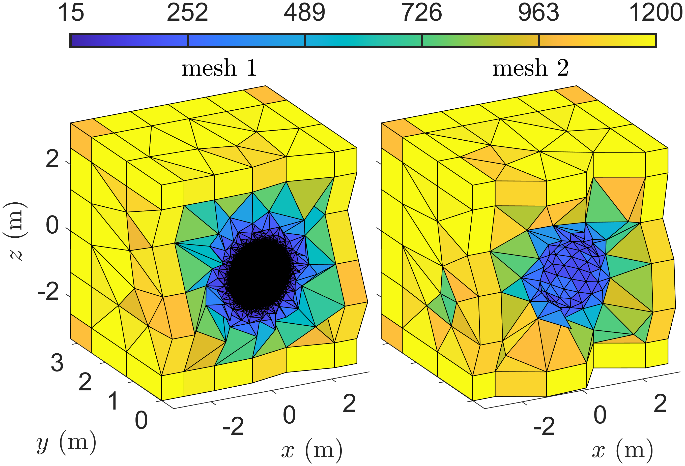
Figure 3: Cross-sections of the computational grids used to approximate scattering from a PEC sphere. The colorbar shows the number of plane wave directions on each element. The major difference is the grid density on the surface of the sphere. This figure shows how wedge and hexahedral elements can be usefully employed in the outer PML layer. In all figures showing grids, the colorbar shows the number of plane wave direction, see Eq. (16), for each element.

Figure 4 shows the modulus of the $y$-component of the scattered electric field $|E_{y}^{s}|$ on the $z=0$ plane. There are clear differences between the results for mesh 1 and mesh 2 with flat facets. These are caused by the coarse surface grid in the second case. However mesh 1 with flat facets, and mesh 2 with a quadratic boundary approximation are in good agreement. As can be seen in Table 2, mesh 2 with quadratic boundary approximation is much cheaper in terms of CPU-time than mesh 1.

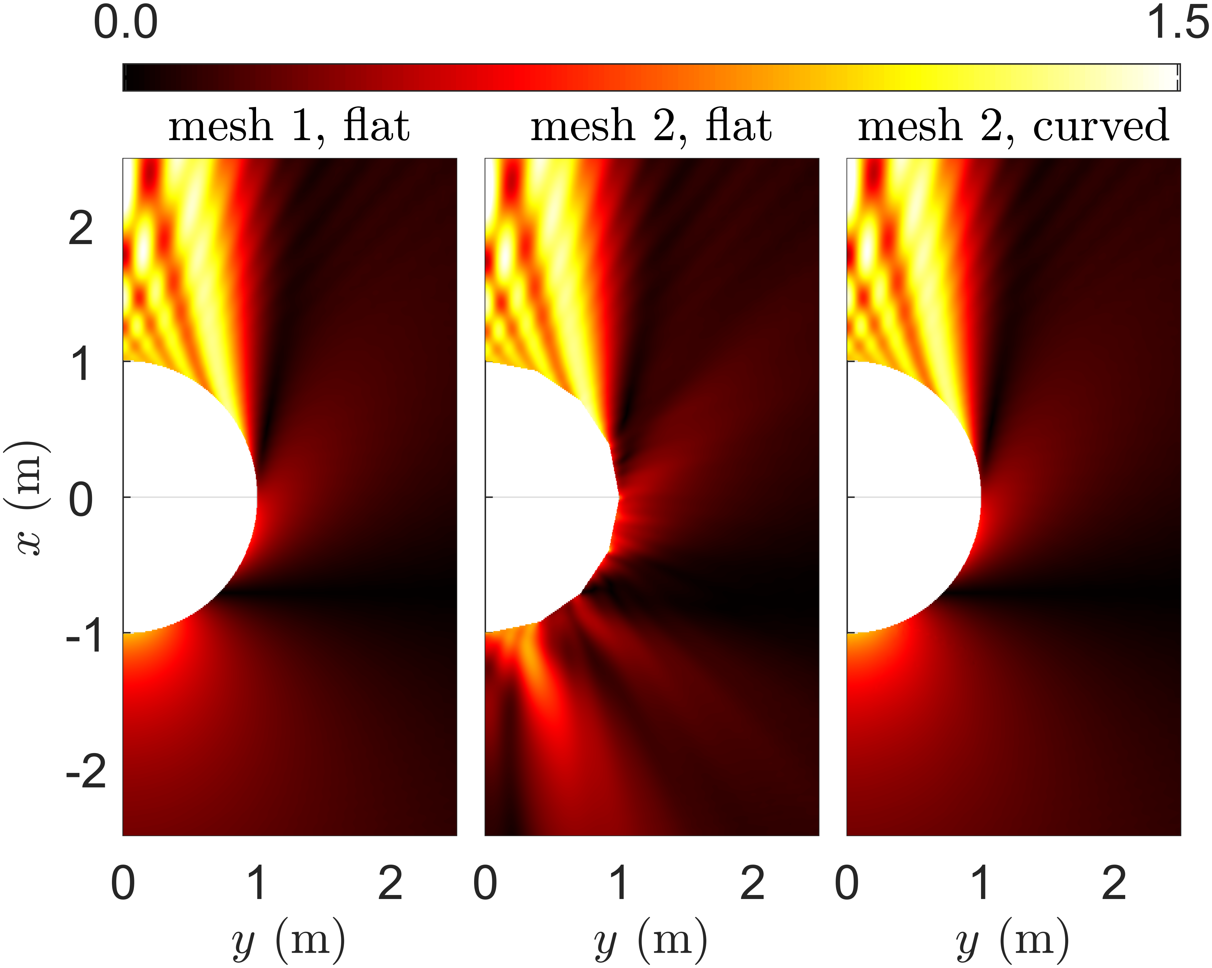
Figure 4: Snapshots of the scattered electric field component $|E_{y}^{s}|$ for the meshes considered here. There is good agreement between mesh 1 and mesh 2 with curved faces. Mesh 2 with flat faces produces unacceptable error due to the coarse boundary approximation.

Very often the far field pattern of the scattered wave [19] is the quantity of interest for these calculations, and in particular the Radar Cross Section (RCS) derived from the far field pattern. In this paper, far field directions are defined in terms of the azimuth angle $\phi$ (^∘) as $(\cos(\phi\pi/180),\sin(\phi\pi/180),0)$.

Figure 5 shows a comparison of the bistatic RCS predicted by the computational experiments with the UWVF and one computed by the Mie series. Clearly mesh 2 with flat facets produces an inaccurate far field pattern, whereas mesh 1 or mesh 2 with curved elements produces much more accurate predictions.

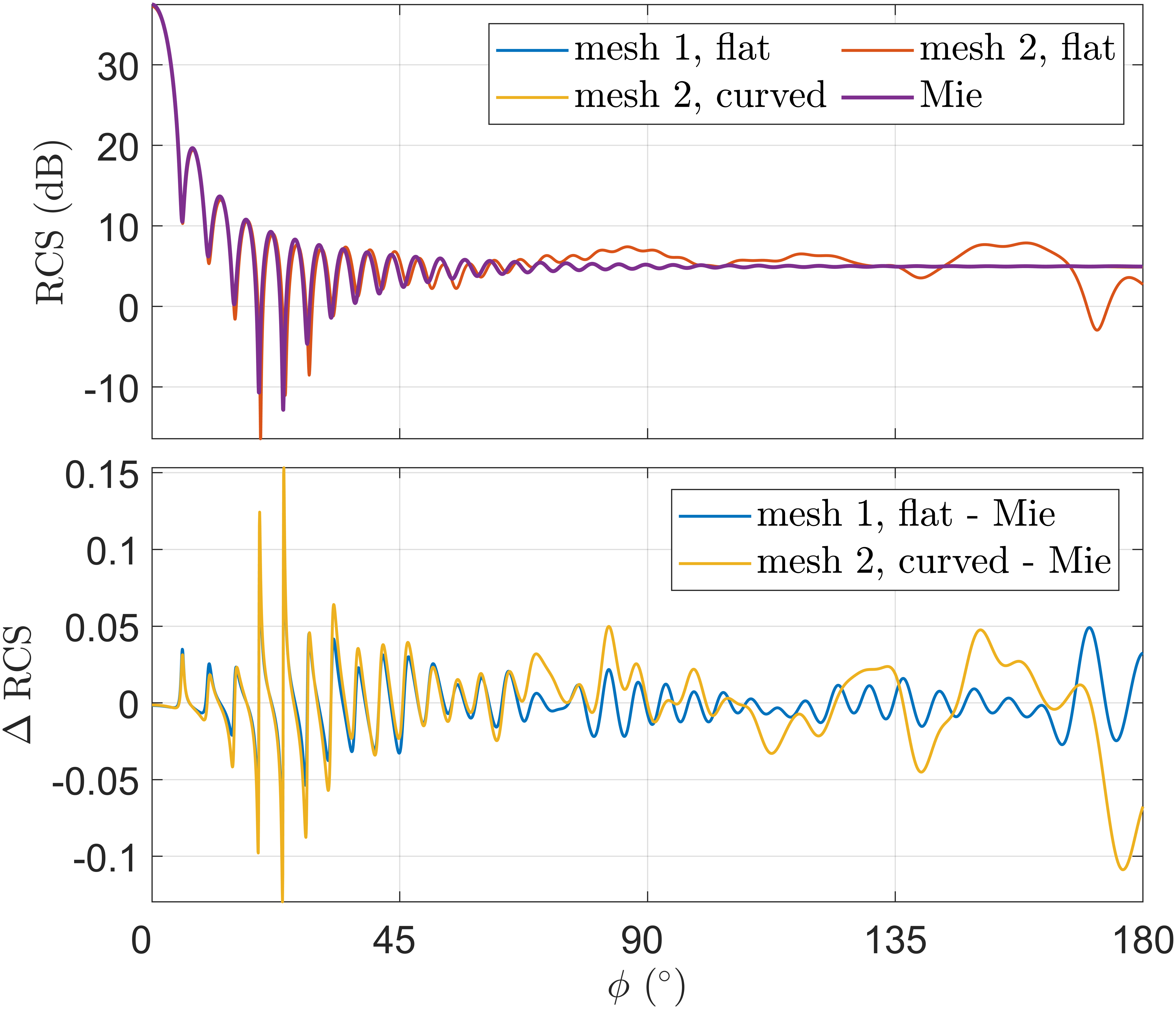
Figure 5: Bistatic RCS at 2 GHz for the PEC sphere. We show the RCS computed using meshes 1 and 2 compared to the Mie series. The bottom panel shows the difference between the numerical solution and the Mie series. Note that the ’Mesh 2, flat - Mie’ curve is omitted from the bottom panel due to its significantly larger amplitude compared to the other two curves.

Table 2: Table giving details for the computational grids for the PEC sphere, and accuracy and timing. See Table 1 for definitions of the reported quantities.

mesh id	surface	$N_{\mathrm{elements}}^{\mathrm{tetra}}$	$N_{\mathrm{elements}}^{\mathrm{wedge}}$	$N_{\mathrm{elements}}^{\mathrm{hexa}}$	$N_{\mathrm{vertices}}$	$h_{\min}$ (cm)	$h_{\max}$ (m)	$N_{\mathrm{DoF}}$	$N_{{\mathrm{iter}}}^{{\mathrm{BiCG}}}$	L2-error (%)	CPU-time (s)
1	flat	122,680	228	56	29,890	0.65	1.93	9,325,028	211	0.21	730
2	flat	1,384	228	56	593	12.79	2.13	1,996,308	73	25.12	355
2	curved	1,384	228	56	593	12.79	2.13	1,996,308	72	0.36	490

4.1.2 An aircraft at X-band frequency

The aircraft model used in this section is derived from a model available in COMSOL (application Simulating Antenna Crosstalk on an Airplane’s Fuselage). We treat the aircraft as a curvilinear perfect conductor. The frequency of the incident field is $f=8$ GHz so $\lambda_{0}=0.03737$ m. The aircraft is 20.5 m or 547 wavelengths long and 17.8108 m or 475 wavelengths wide. A perfectly matched layer with a thickness of $5\lambda_{0}$ is added to each side of the cuboid computational domain with side lengths (16.3334, 16.3334, 4.4826) m.

For generating the computational grid, curved elements and a mesh size parameter of $h_{\mathrm{s}}=3\lambda_{0}$ were employed on the aircraft’s surface. Because we can use 10$\lambda_{0}$ sized elements away from the boundary, the entire grid can be created on a standard office computer. The grid consists of 697,783 tetrahedral elements with 142,731 vertices covering the computational domain. The surrounding PML layer is discretized using 413 hexahedral and 14,904 wedge elements. In addition, for this grid $h_{\min}=1.72$ cm and $h_{\max}=0.55$ m. The number of degrees of freedom $N_{\mathrm{DoF}}$ is 685,245,422.

In Fig. 6, the computational grid on the aircraft’s surface is depicted, along with the grid in two planes: $z=-1$ m and $x=0$ m.

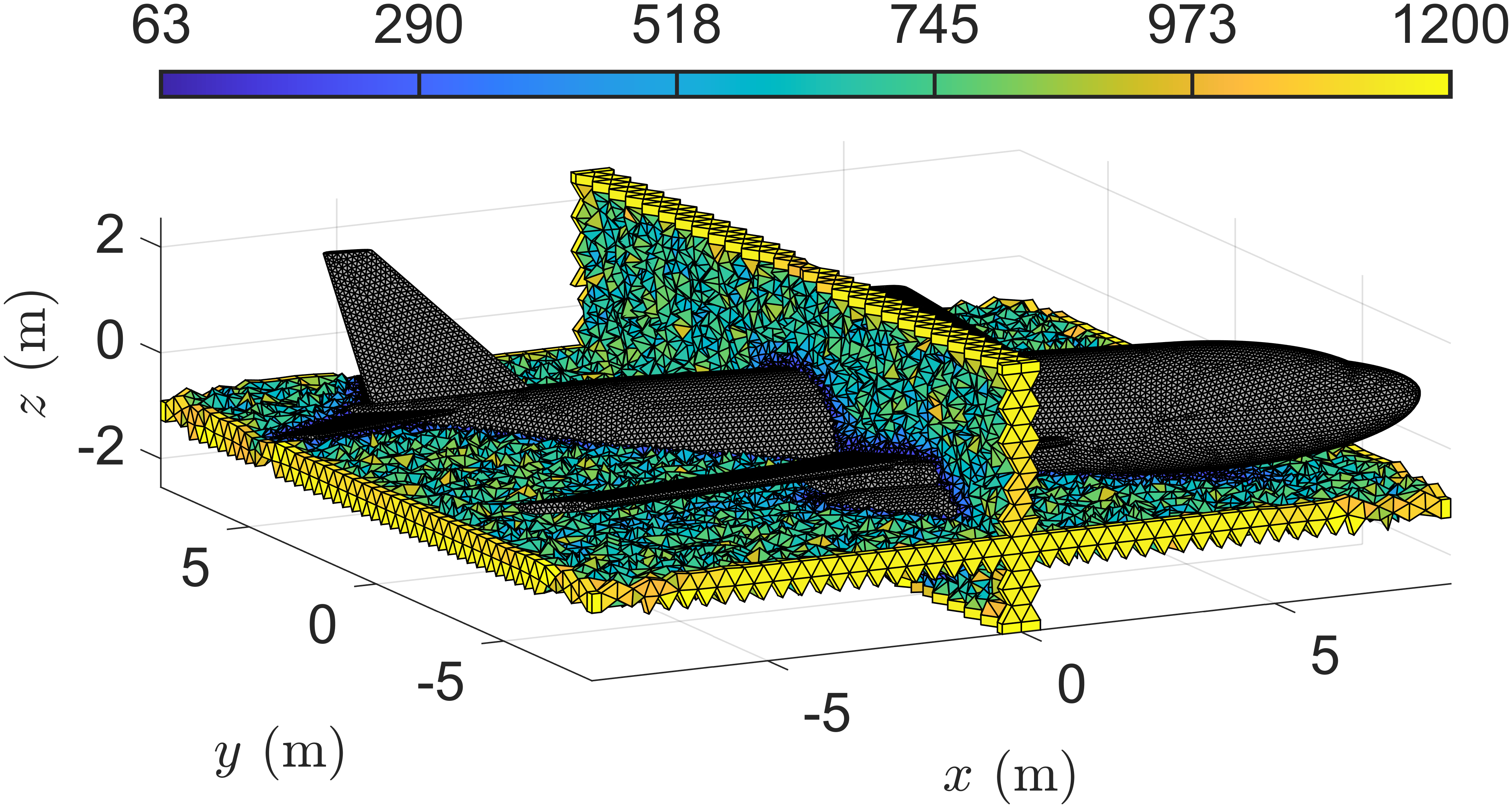
Figure 6: Surface triangulation for the aircraft and tetrahedral, hexahedral, and wedge elements on two planes. The colorbar shows the number of plane waves per element.

For this numerical experiment we used the supercomputer Mahti. When we tried this example storing the matrices $C$ and $D$ as usual (see Eq. (9)), we ran out of memory. An estimate for the memory requirement for solving the problem by keeping all necessary matrices in memory is 68 terabytes. The low memory version relaxes this memory requirement by a factor of 0.2. So we switched to the low memory version described in Section 3.5 to compute the results shown here. In Mahti, we used a total of 200 computing nodes and 100 CPU units per node. The total time for the calculation was 18 hours, including building the system matrix $D$, and then iteratively reaching the requested solution accuracy. The BICGstab algorithm took a total 437 iterations.

Figure 7 shows the scattered electric field $|E_{y}^{s}|$ on the $x=0$, $y=0$, $z=0$ planes. Fig. 8 shows the RCS in a full azimuth angle range $\phi\in[0,360]^{\circ}$.

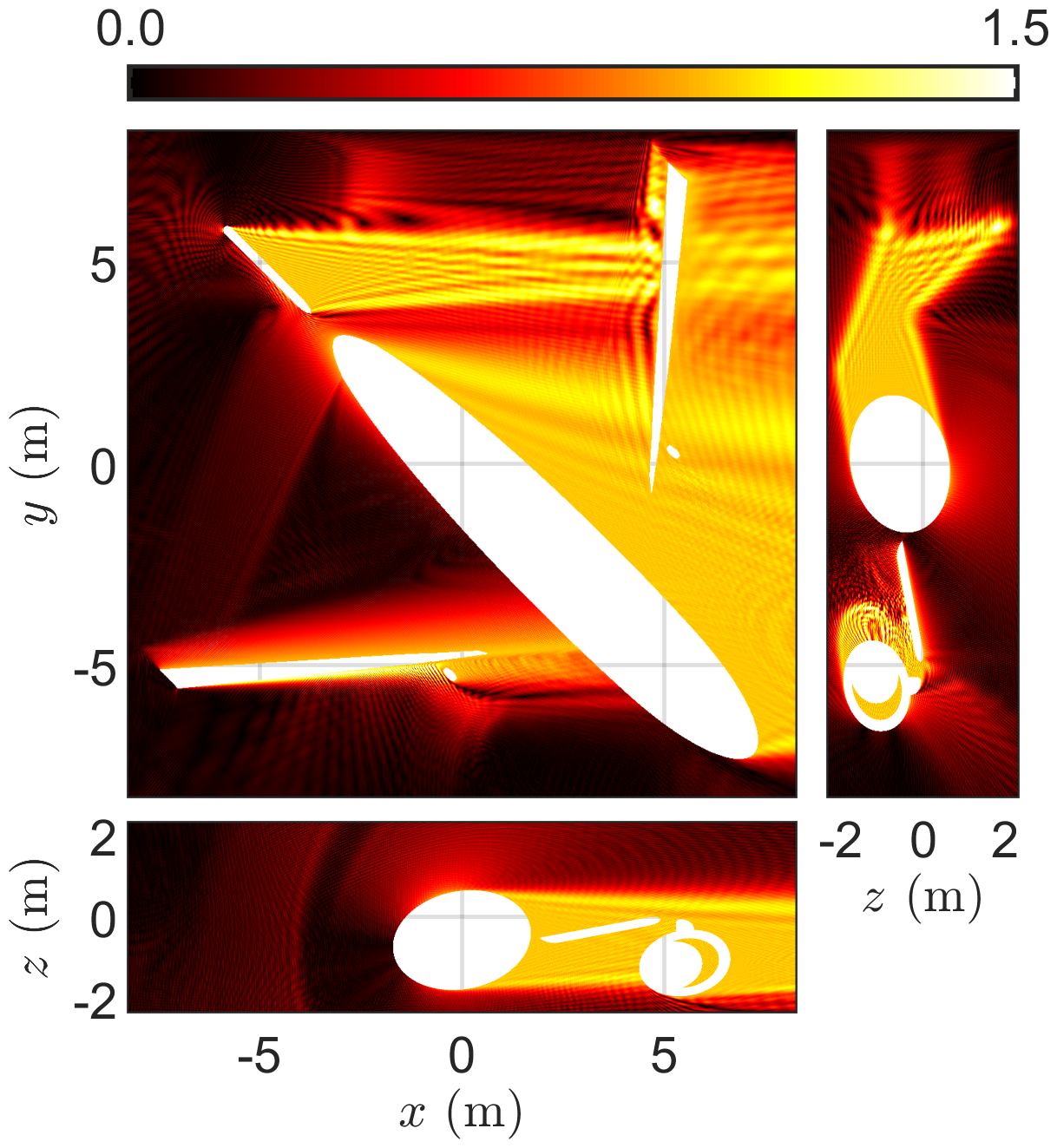
Figure 7: Snapshots of the scattered electric field $|E_{y}^{s}|$ for the aircraft model. In the top left panel we show results in the $x-y$ plane at $z=0$, top right is in the $z-y$ plane at $x=0$ and bottom left is in the $x-y$ plane at $z=0$. Clearly a strong shadow region and multiple reflections are evident.

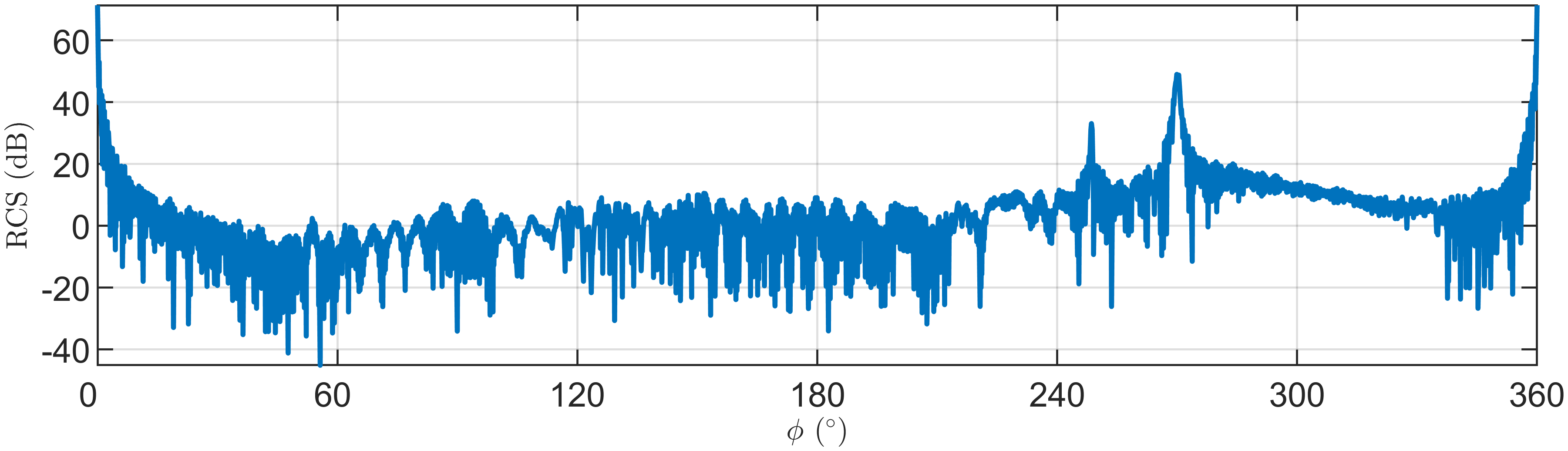
Figure 8: Bistatic RCS for the aircraft at 8 GHz.

4.2 Resistive sheets

4.2.1 Salisbury screen

We next model a “Salisbury screen” (W. W. Salisbury, U. S. Patent US2599944 A 1952). For simplicity, assume $\epsilon_{\mathrm{r}}=\mu_{\mathrm{r}}=1$. Our standard incident field (10) propagates normally to a resistive sheet at $x=-H$, $H>0$ backed by a PEC surface at $x=0$.

To the left of the resistive sheet the total electric field is

$${\bf E}_{-}=\left(\begin{array}[]{c}0\\ 1\\ 0\end{array}\right)\exp(i\kappa x)+\left(\begin{array}[]{c}0\\ R_{2}\\ 0\end{array}\right)\exp(-i\kappa x),\;x<-H,$$

where $(0,R_{2},0)^{T}$ is the polarization of the reflected wave. Between the sheet and the PEC surface, where $-H<x<0$,

$${\bf E}_{+}=\left(\begin{array}[]{c}0\\ q_{0,2}\\ 0\end{array}\right)\exp(i\kappa x)+\left(\begin{array}[]{c}0\\ q_{1,2}\\ 0\end{array}\right)\exp(-i\kappa x).$$

Here $(0,q_{0,2},0)^{T}$ and $(0,q_{1,2},0)^{T}$ are the polarizations of the left and right going waves respectively in the gap $-H<x<0$.

Imposing the PEC boundary condition at $x=0$ and the resistive sheet transmission conditions (11)-(12) at $x=-H$ shows that

$$\mathit{R_{2}} = -\frac{\left(i\left(\eta-1\right)\sin\!\left(\kappa H\right)-\cos\!\left(\kappa H\right)\right)\exp\left(-2i\kappa H\right)}{i\left(\eta+1\right)\sin\!\left(\kappa H\right)-\cos\!\left(\kappa H\right)},$$

$$\mathit{q_{0,2}} = \frac{\exp\left(-i\kappa H\right)}{-i(\eta+1)\sin\!\left(\kappa H\right)+\cos\!\left(\kappa H\right)},$$

$$\mathit{q_{1,2}} = \frac{\exp\left(-i\kappa H\right)}{i\left(\eta+1\right)\sin\!\left(\kappa H\right)-\cos\!\left(\kappa H\right)}.$$

For given $\kappa$, $H$, and $\eta$ we can compute total field in each region and compare to the analytic solution. As is well known, one choice of $\eta$ gives $R_{2}=0$:

$$\eta=1-i\cot(\kappa H).$$

A particularly interesting case occurs when $\cot(\kappa H)=0$ or $H=\pi/(2\kappa)$. Recalling that the wavelength of the radiation is $\lambda_{0}=2\pi/\kappa$, we see that zero reflection occurs when $H=\lambda_{0}/4$.

To test the UWVF for resistive sheets, we use a rectangular parallelepiped computational region with faces normal to the coordinate directions (see Fig. 9). The rightmost face $x=0$ is PEC ($Q=-1$) the left-most face is an ABC with $Q=0$ where we use a non-homogeneous absorbing boundary condition to excite the plane wave. There is no need for a PML since the solution is a wave propagating orthogonally to the absorbing boundary.

On the remaining faces $Q=\pm 1$ chosen so that the incident plane wave propagates along the box without distortion. We take the radiation to have frequency $f=2$ GHz and place the resistive sheet one quarter wavelength ($H=3.75$ cm) from the PEC surface. Figure 9 shows a surface of the grid used in the computations. In this case, the grid consists of 136 tetrahedral elements with 51 vertices. In addition, $h_{\min}=3.33$ cm, $h_{\max}=16.18$ cm, and $N_{\mathrm{DoF}}=9,946$.

Results are shown in Fig. 10. We plot the magnitude of the $y$-component of the total field as a function of $x$ when $y=z=7.5$ cm. Choosing $\eta=1$ the magnitude of the field is flat to the left of the resistive sheet showing that this choice of $\eta$ gives rise to no reflected wave. However when $\eta=0.5$ the non-constant magnitude of the total field indicates that a reflected wave is present to the left of the sheet.

In this example just two plane waves per element would suffice to compute the solution, but our code is not tuned to this example and chooses the number of directions as if this is a general Maxwell problem via the condition number heuristic in Appendix A.

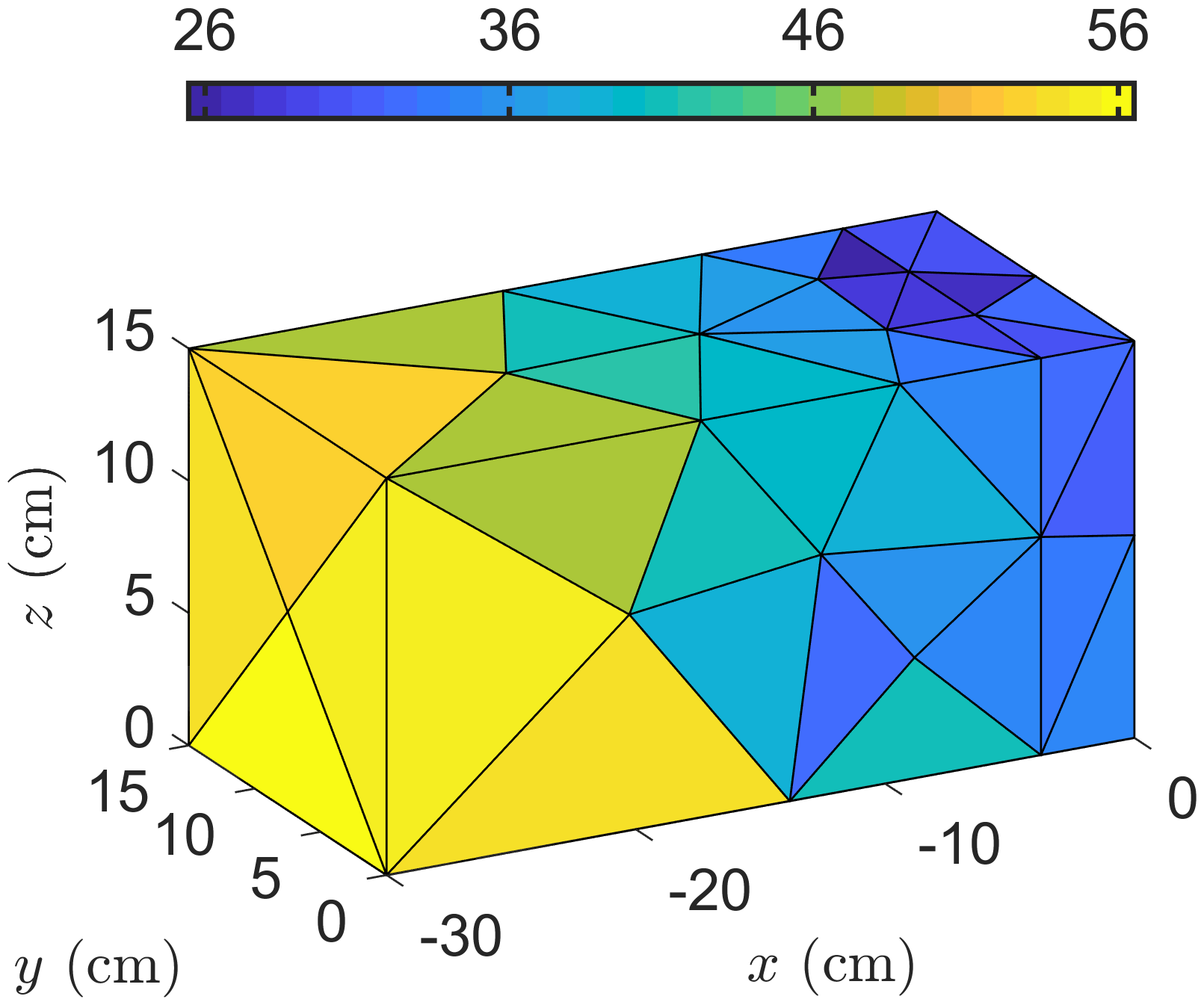
Figure 9: Computational grid for the Salisbury screen, showing smaller elements between the screen and PEC surface, expanding away to the left.

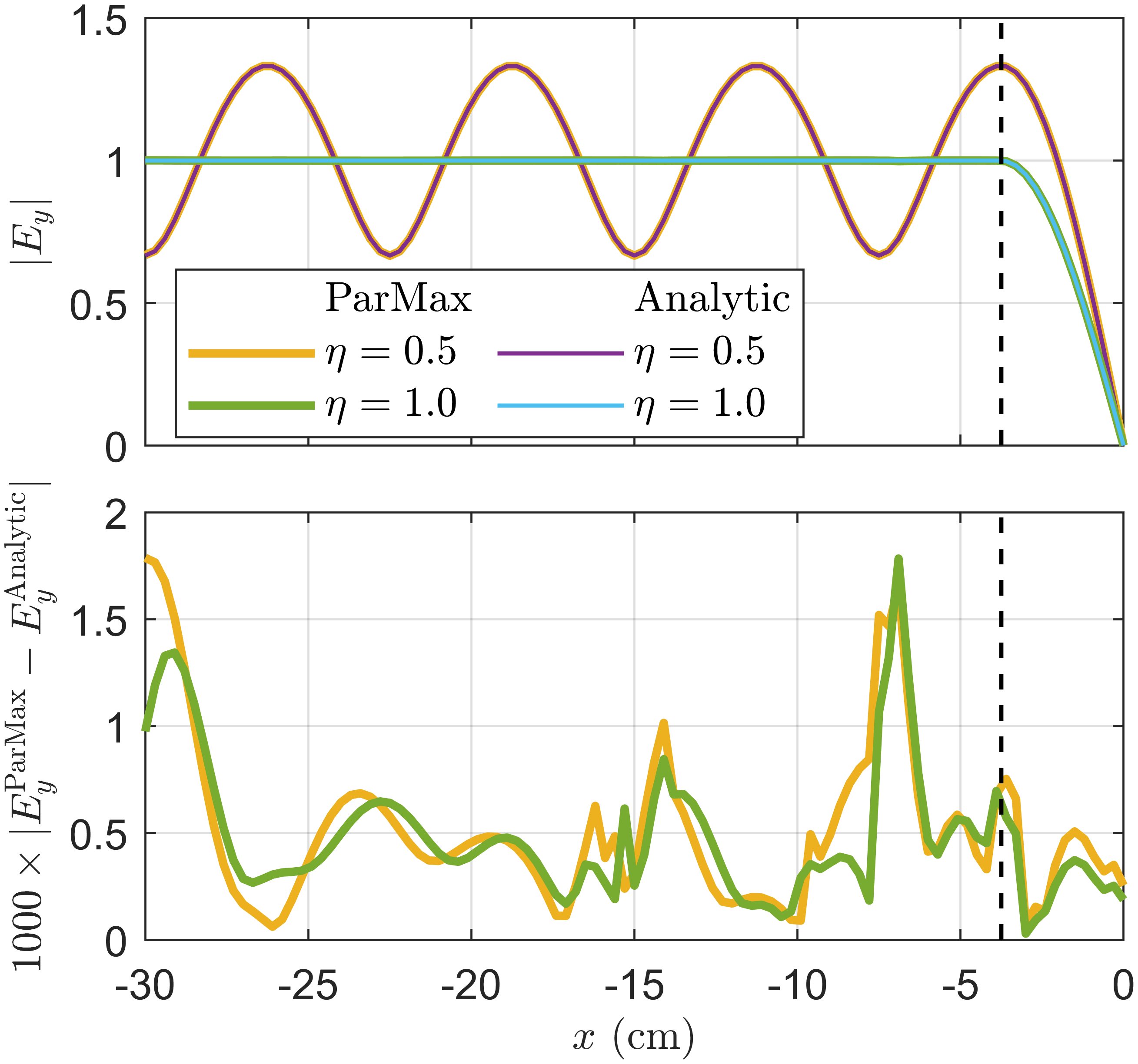
Figure 10: Magnitude of the $y$-component of the total electric field $E_{y}$ as a function $x$ with $y=z=7.5$ cm with $\eta=1$ and $\eta=0.5$, together with the analytic solution. The vertical dashed line marks the location of the resistive sheet. To the left of the sheet, no reflected wave is evident when $\eta=1$ whereas a reflected wave is indicated when $\eta=0.5$. The bottom panel shows the absolute value of the difference between the numerical and analytic solutions, with the difference multiplied by a factor of 1,000.

4.2.2 Sphere with resistive sheet

In this second experiment with resistive sheets, a PEC sphere with a radius of 1 meter is placed at the origin of a cube $[-1-15\lambda_{0},1+15\lambda_{0}]^{3}$. Surrounding this sphere is a spherical resistive sheet of radius $1+\lambda_{0}/4$ and surrounding both is an artificial sphere of radius $1+\lambda_{0}$. Outside this artificial sphere we compute the scattered field, and inside the total field (see Section 3.2). The incident field then gives rise to a source on the artificial boundary as detailed in Section 3.2. A PML with a thickness of $5\lambda_{0}$ is applied to the inside each side of the cube, and the frequency of the incident field is set at $f=2$ GHz. The incident field gives rise to a source located on the sphere.

To generate the computational grid, we utilized curved elements and a mesh size parameter of $h_{\mathrm{s}}=2\lambda_{0}$ on the PEC and resistive sheet surfaces. The grid comprises of 428 wedge elements (representing the domain between the resistive sheet and PEC sphere) and 7,589 tetrahedral elements that cover the main domain of interest. Furthermore, the surrounding PML layer is discretized using a combination of 104 hexahedral and 936 wedge elements. The entire grid is composed of 2,550 vertices, with $h_{\min}=3.75$ cm and $h_{\max}=1.48$ m. A cross-section of the computational grid is shown in Fig. 11. In this case, the number of degrees of freedom $N_{\mathrm{DoF}}=4,599,234$.

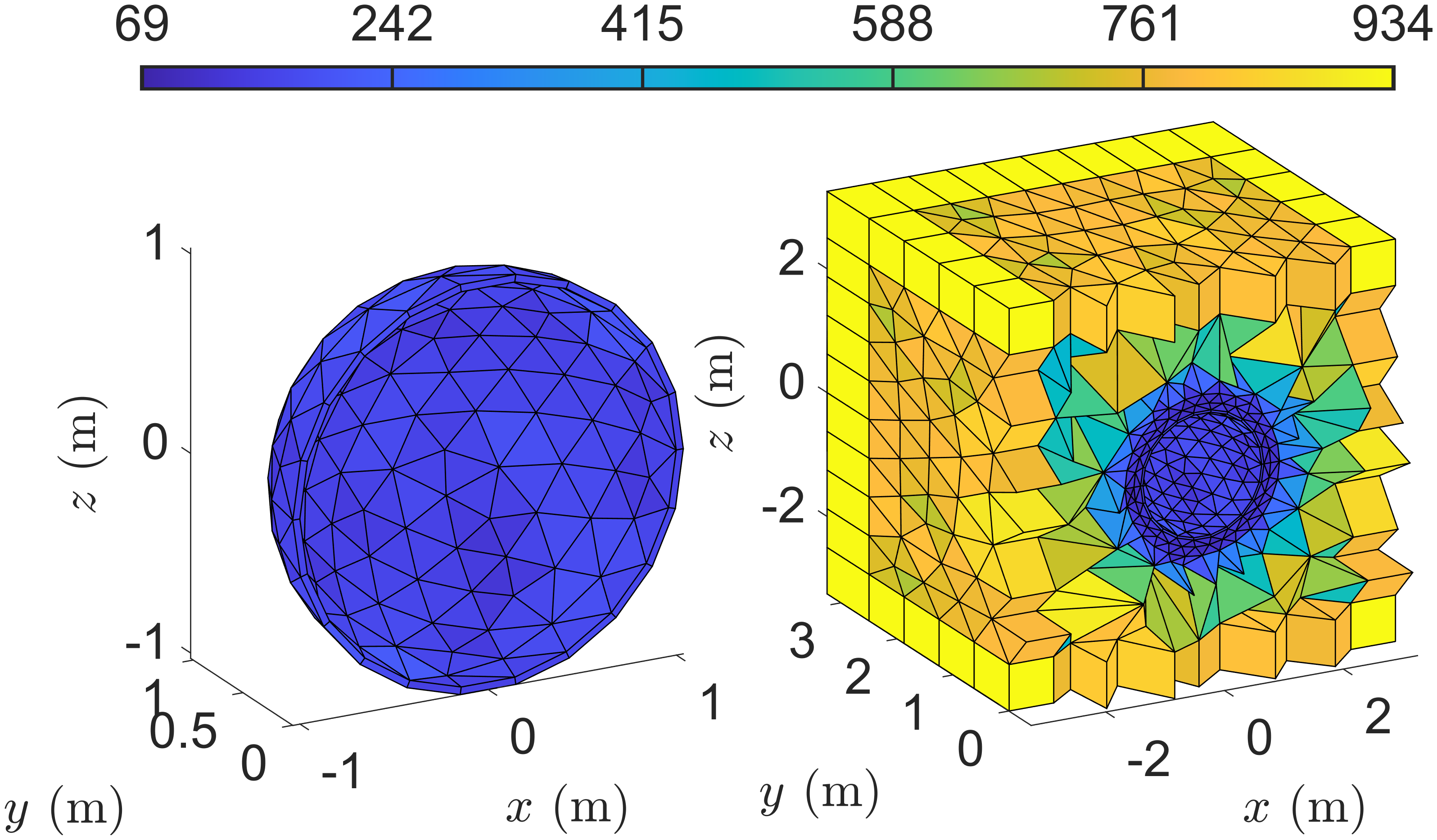
Figure 11: Left: 428 wedge elements forming the interior of the resistive sheet outside the PEC surface. Right: A cross-section of the overall computational grid.

We used the supercomputer Puhti with a total of 5 computing nodes and 10 CPU units per node to solve the three configurations for different resistive sheet parameters $\eta$. It took 18 ($\eta=0$), 17 ($\eta=0.5$), and 17 ($\eta=1.0$) minutes CPU-time respectively to build the system matrices and then reach the solution with BICGstab. The solution was achieved after 194 iterations for $\eta=0$, 169 iterations for $\eta=0.5$, and 172 iterations for $\eta=1.0$.

In Fig. 12, the total field component $\Re(E_{y})$ on the plane $z=0$ is shown for three choices of $\eta$. We can no longer expect invisibilty since the screen is curved, but it is evident that backscattering is decreasing as $\eta$ increases. This is seen more clearly in Fig. 13 where we show the RCS in each case.

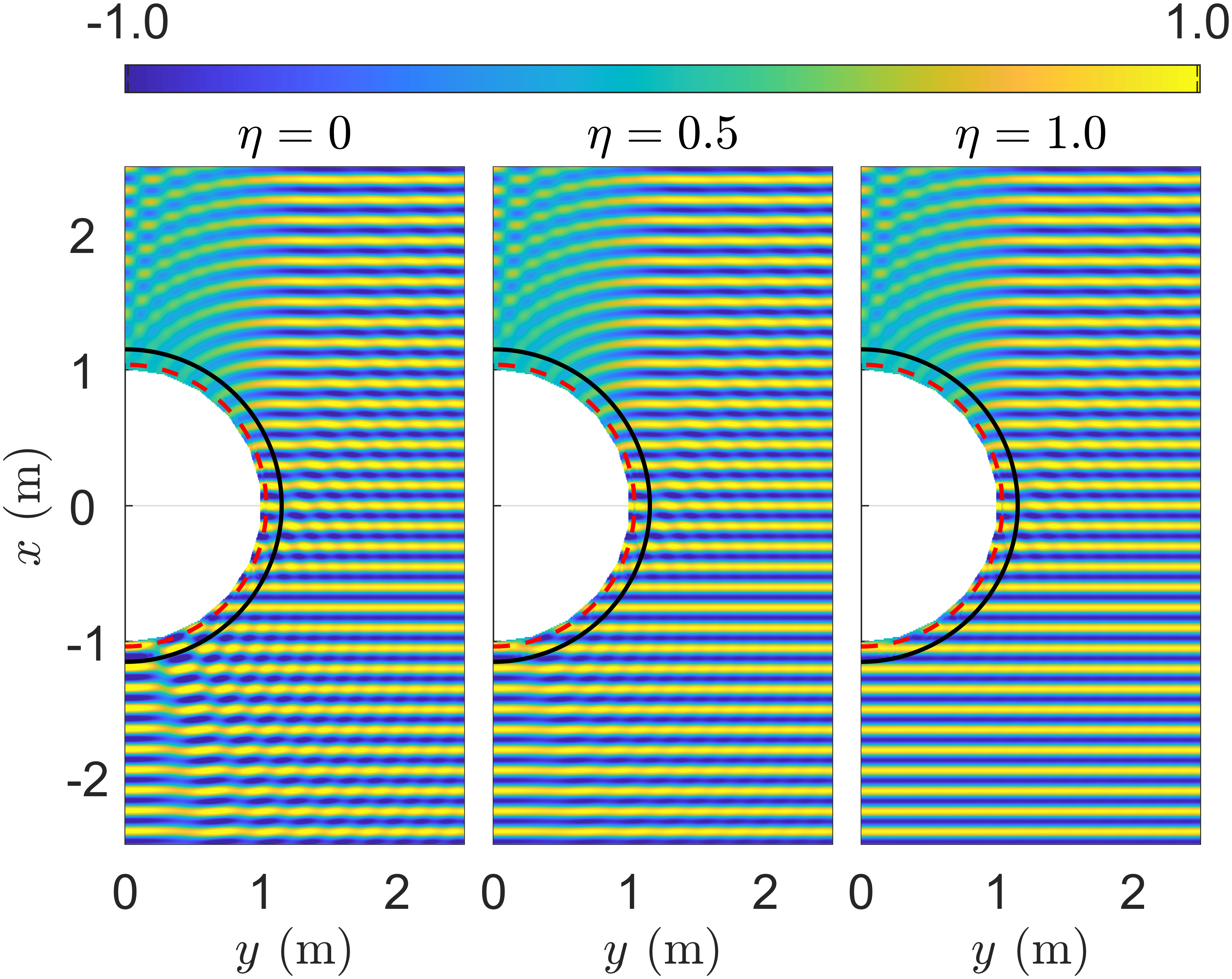
Figure 12: Snapshots of the total electric field $\Re(E_{y})$ for the three choices of resistive sheet parameter $\eta$ (left: $\eta=0$, middle: $\eta=0.5$ and right: $\eta=1$). The dashed red line marks the resistive sheet interface and the solid black line the artificial interface used to introduce the incident wave. Backscattering appears less for $\eta=1$ compared to $\eta=0.5$ or the pure PEC sphere.

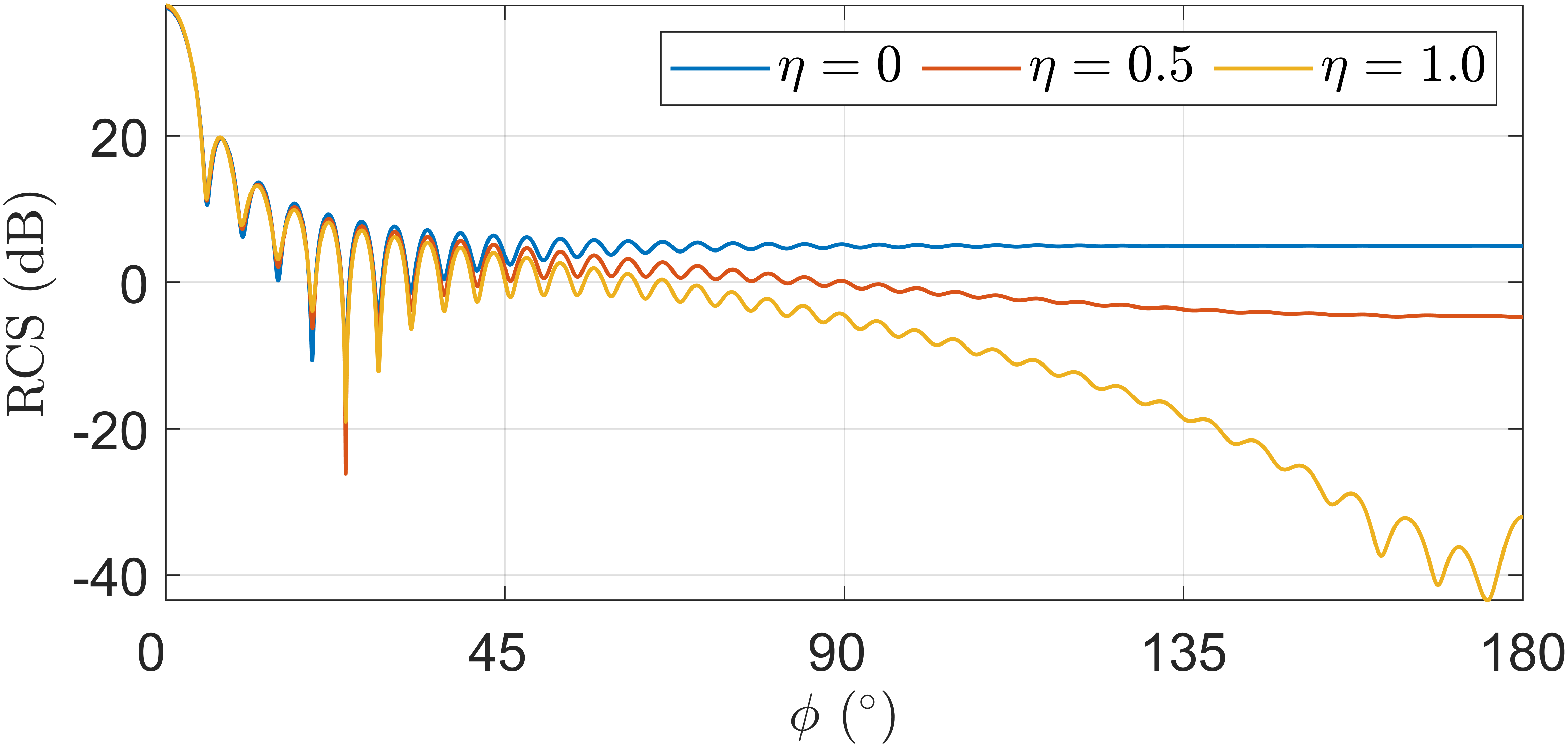
Figure 13: Bistatic RCS for the PEC sphere and resistive sheet example at 2 GHz. The decreased backscattering due to the resitive sheet covering the sphere at $\eta=1$ is clearly seen.

4.3 Heterogeneous models

4.3.1 A dielectric sphere

In this experiment, a penetrable sphere with a radius of 1 meter is centered at the origin inside the cube $[-1-15\lambda_{0},1+15\lambda_{0}]^{3}$, where $\lambda_{0}$ is the wavelength in vacuum. For the penetrable sphere, we assume $\epsilon_{\mathrm{r}}=1.5+0.5i$ and $\mu_{\mathrm{r}}=1$, while we select vacuum parameters in other domains. The frequency of the incident field is $f=2$ GHz and a PML with thickness of $5\lambda_{0}$ is used on each side of the cube. An artificial spherical boundary with radius $1+\lambda_{0}$ is used to separate a scattered field region outside and a total field region inside this surface. The scattered-total field formulation in Section 3.2 is used to introduce a source on the artificial boundary.

We utilised curved elements and a mesh size parameter of $h_{\mathrm{s}}=3\lambda_{s}$, where $\lambda_{s}$ is a measure of the wavelength in the penetrable sphere computed using $\kappa_{\mathrm{abs}}$ defined in Appendix A. Figure 14 shows cross-sections of the computational grids. To solve this problem, we used the supercomputer Puhti with a total of 7 computing nodes and 40 CPU units per node. More detailed information on the computations, including information on the grids and CPU time, is given in Table 3.

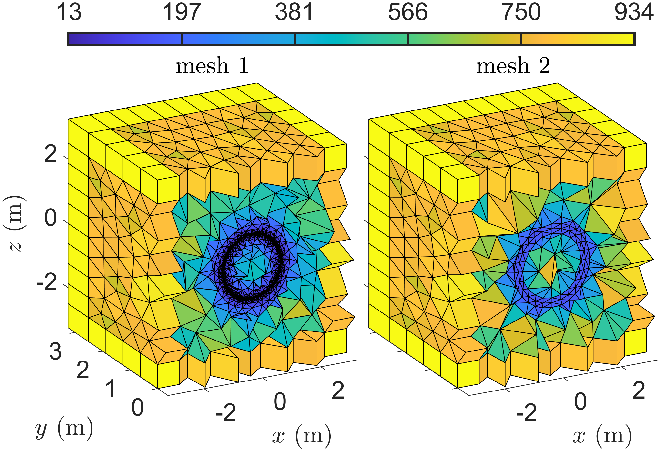
Figure 14: Cross-section of the computational grid for the penetrable sphere case.

In Fig. 15, we show the total field component $\Re(E_{y})$ on the $z=0$-plane for the two meshes. As expected (see also Table 3), mesh 2 with curved face elements produces a solution comparable to mesh 1, but faster. The accuracy of the far field pattern is compared to the Mie series solution in Fig. 16, and again demonstrates that mesh 1 and mesh 2 with curved faces give comparable results.

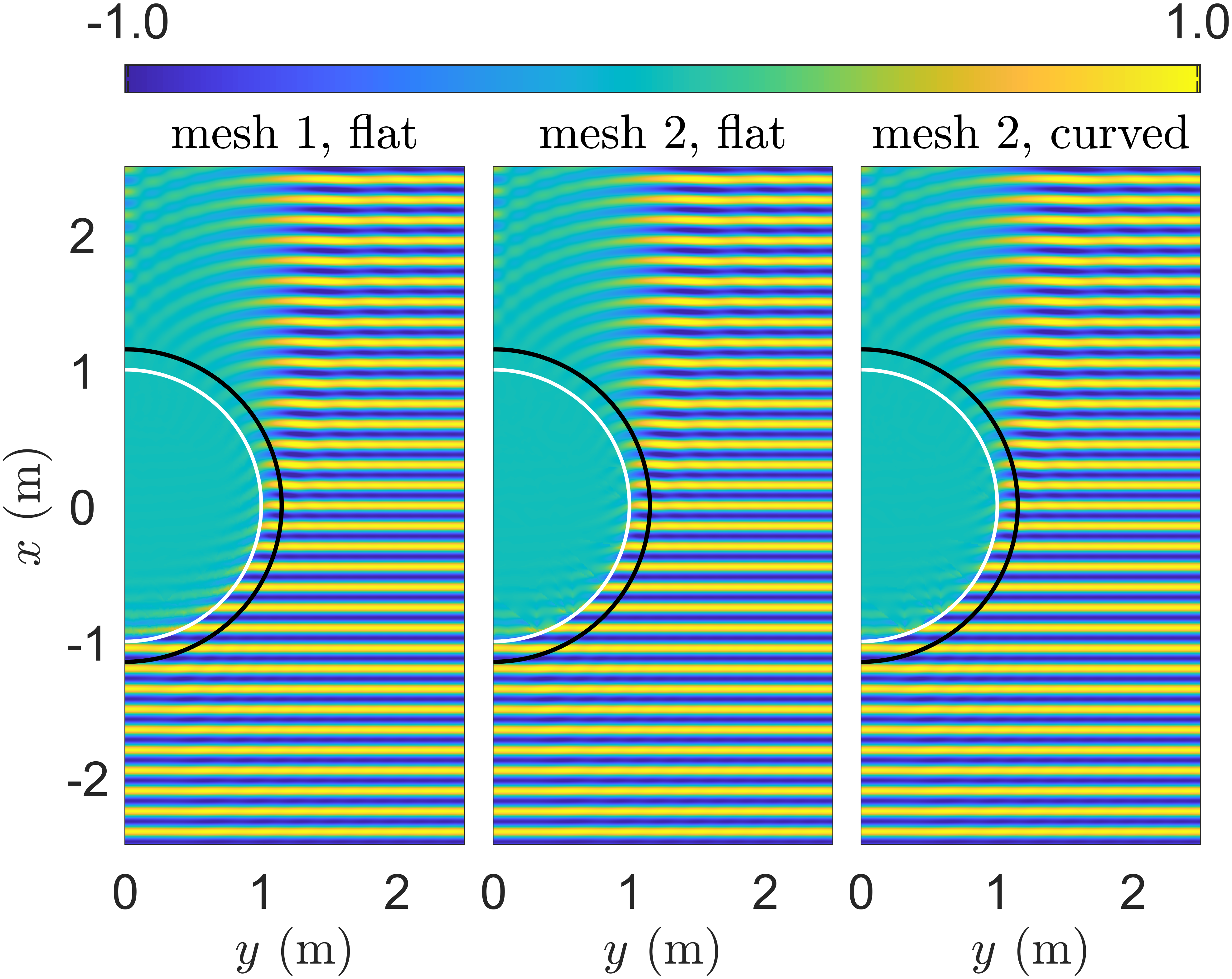
Figure 15: Snapshots of the electric field $\Re(E_{y})$ on the $z=0$ plane for the penetrable sphere. The solid white line shows the material interface and the solid black line marks the artificial interface used to introduce the incident wave.

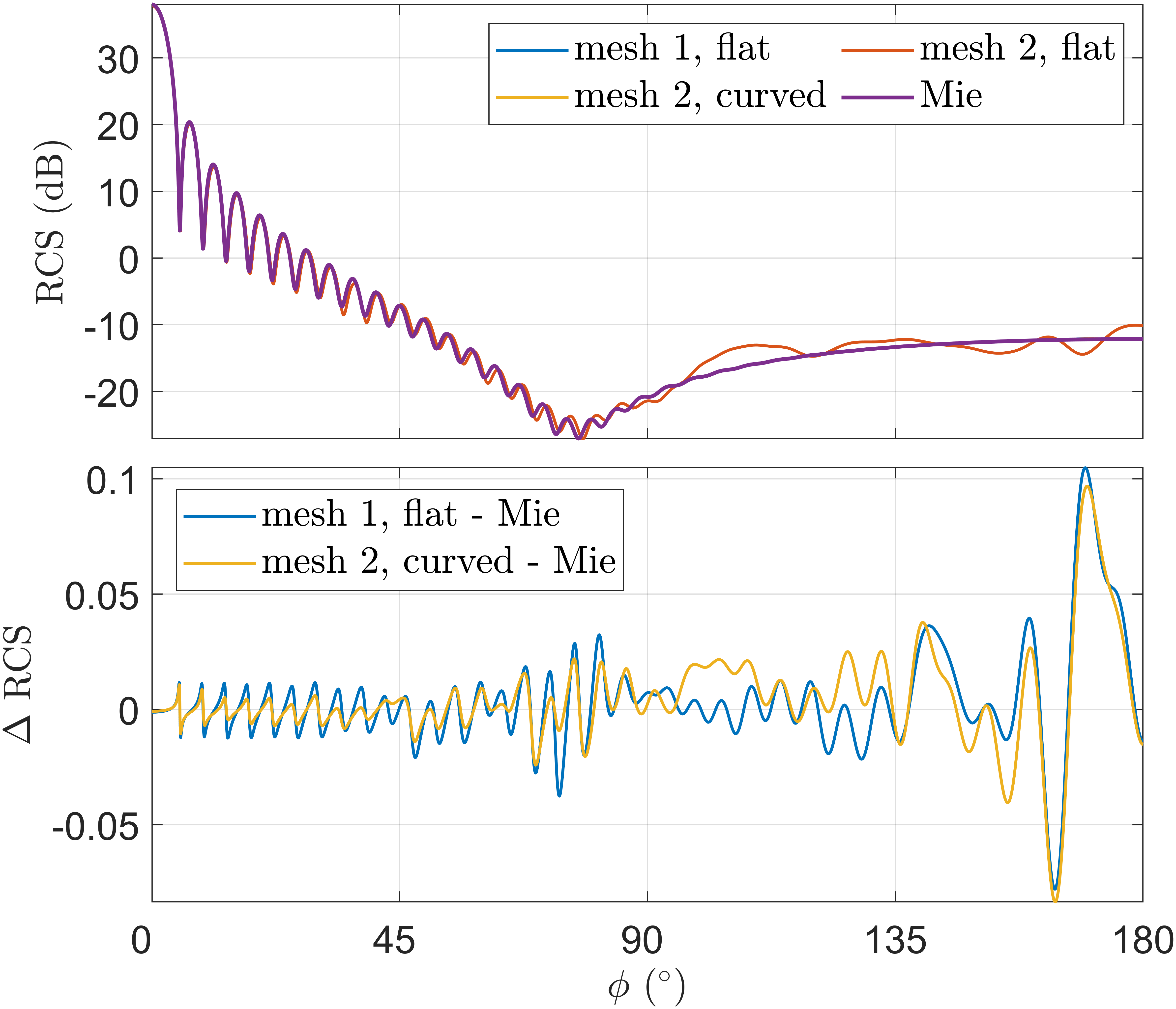
Figure 16: Bistatic RCS for the penetrable sphere at 2 GHz, otherwise the layout is the same caption as for Fig. 5.

Table 3: Details of the computational results for the penetrable sphere. See Table 1 for definitions of the reported quantities.

mesh id	surface	$N_{\mathrm{elements}}^{\mathrm{tetra}}$	$N_{\mathrm{elements}}^{\mathrm{wedge}}$	$N_{\mathrm{elements}}^{\mathrm{hexa}}$	$N_{\mathrm{vertices}}$	$h_{\min}$ (cm)	$h_{\max}$ (m)	$N_{\mathrm{DoF}}$	$N_{{\mathrm{iter}}}^{{\mathrm{BiCG}}}$	L2-error (%)	CPU-time (s)
1	flat	337,550	936	104	59,053	0.65	1.30	21,633,354	187	0.14	346
2	flat	7,100	936	104	2,161	7.80	1.42	4,640,348	90	7.85	162
2	curved	7,100	936	104	2,161	7.80	1.42	4,640,348	88	0.14	234

For a comparison of ParMax with edge finite elements in the case of the dielectric sphere, see Appendix B.

4.3.2 A plasma sphere

In this second experiment for penetrable objects, we assume a penetrable sphere with a radius of 0.25 meter is centred at the origin of a cube $[-0.25-15\lambda_{0},0.25+15\lambda_{0}]^{3}$. The material in the sphere is assumed to be a plasma modelled by setting $\epsilon_{\mathrm{r}}=-1.5+0.5i$ and $\mu_{\mathrm{r}}=1$. The frequency of the incident field is $f=2$ GHz and a perfectly matched layer with thickness of $5\lambda_{0}$ is used inside each side of the cube. The source is introduced on an artificial spherical surface of radius $0.25+\lambda_{0}$.

We utilise curved elements and a mesh size parameter $h_{\mathrm{s}}=3\lambda_{s}$, where $\lambda_{s}$ denotes the wavelength in the penetrable sphere, on the material discontinuity surface. The grid comprises of 2,959 tetrahedral elements that cover the main domain of interest. Furthermore, the surrounding PML layer is discretized using a combination of 92 hexahedral and 768 wedge elements. The entire grid has 1,304 vertices, with $h_{\min}=5.88$ cm and $h_{\max}=1.30$ m. Here, the degrees of freedom number $N_{\mathrm{DoF}}$ is 2,234,416.

We used the supercomputer Puhti with a total of 5 computing nodes and 10 CPU units per node to solve the problem. It took 427 seconds from each CPU unit to build the system matrices $C$ and $D$ and then reach the solution with 103 bi-conjugate iterations. Snapshots of the total field are shown in Fig. 17. In Fig. 18 we show the computed RCS which shows remarkable agreement with the Mie series solution.

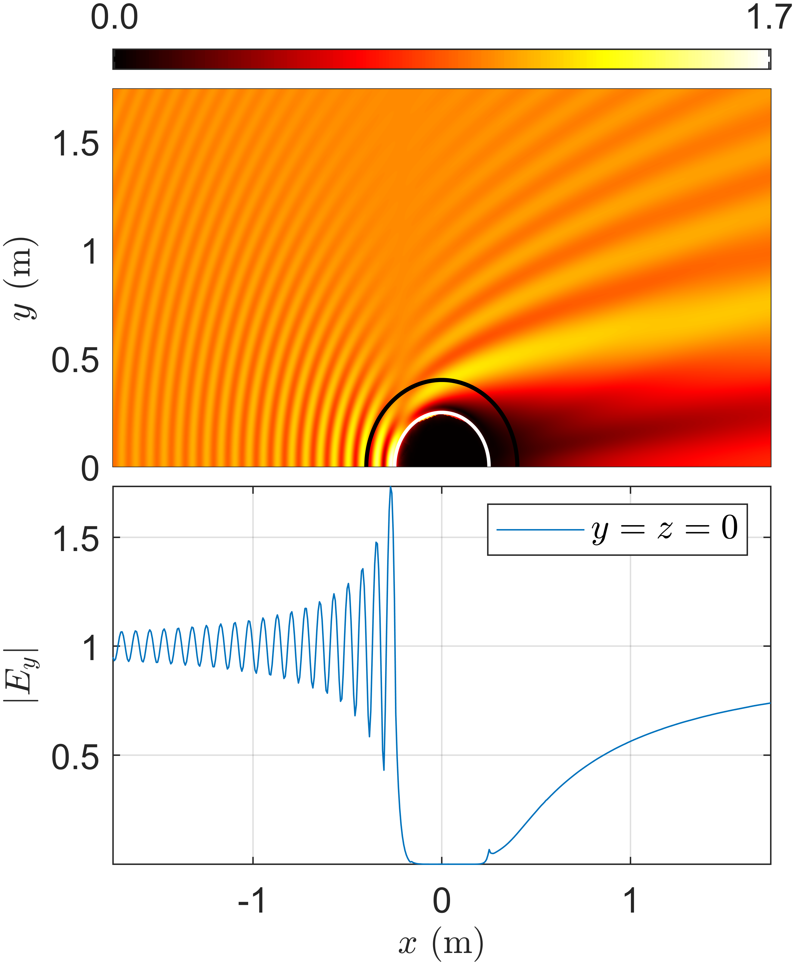
Figure 17: Snapshots of the total electric field. Top panel: a contour plot of $|E_{y}|$ in the plane $z=0$. The solid white line shows the interface between vacuum and the plasma sphere. The solid black line marks the interface used to introduce the incident wave. Bottom panel: a plot of $|E_{y}|$ along the line $y=z=0$.

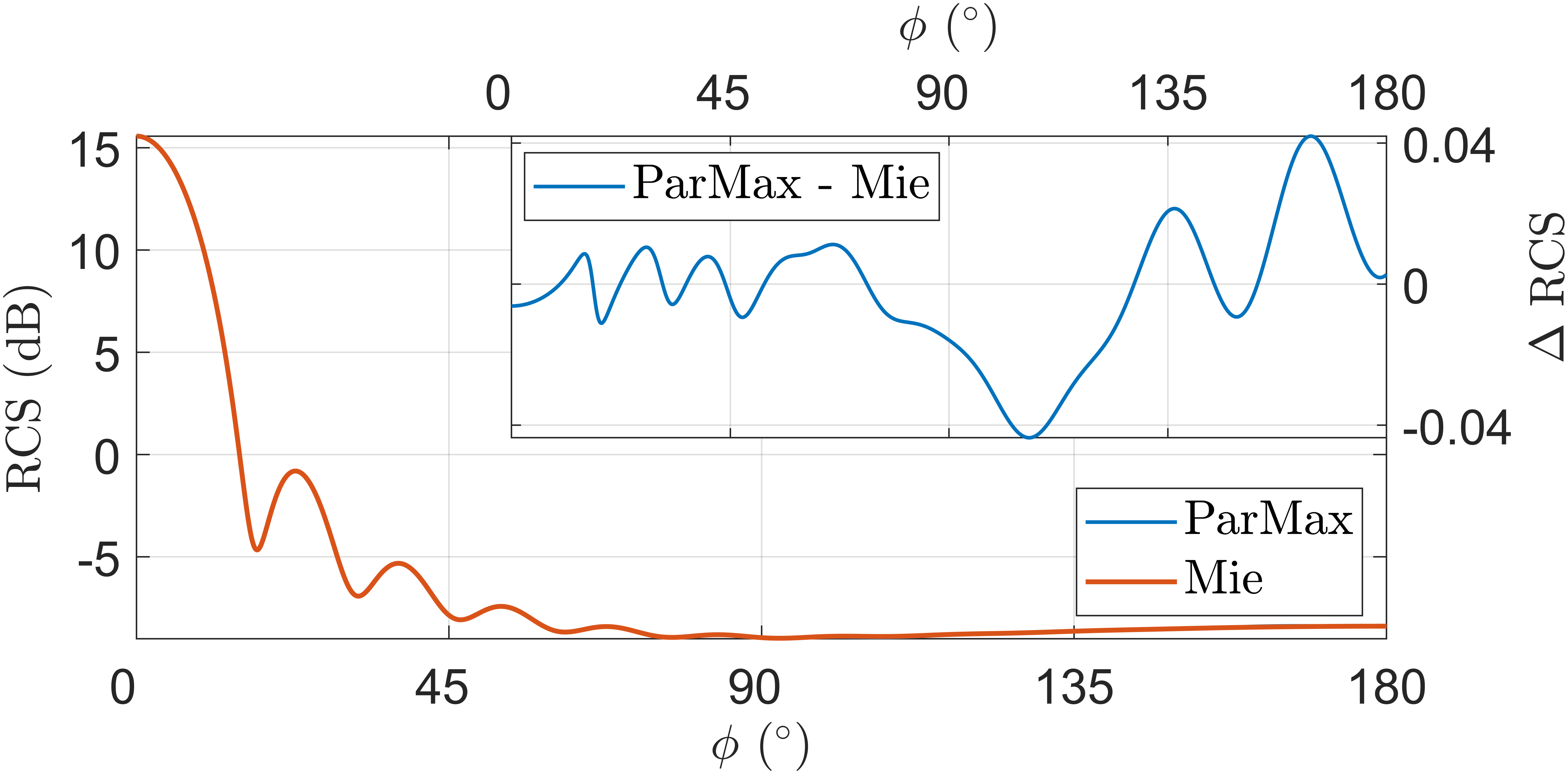
Figure 18: Bistatic RCS for the plasma sphere at 2.0 GHz, comparing the computed RCS and Mie result. Top right corner shows the difference between the numerical and Mie series.

5 Conclusion

In this study, we explored and extended the Ultra-Weak Variational Formulation (UWVF) applied to the time-harmonic Maxwell’s equations. Our research findings led to important contributions that enhance the efficiency and applicability of the UWVF method for solving electromagnetic wave problems.

The paper shows a series of numerical examples validating the effectiveness of the new enhancements. Scattering problems from PEC objects were considered, highlighting the benefits of curved elements, different element types, and the low-memory version of the software. The applicability was further demonstrated through simulations of scattering from an full size aircraft, emphasising its potential for real-world industrial scenarios.

This paper has not only extended the capabilities of the UWVF for electromagnetic wave problems but has also provided a comprehensive set of numerical results to underline the practical significance of these advancements. The integration of curved elements, various element shapes, and resistive sheets collectively contribute to the method’s robustness and utility, making it a valuable tool for addressing complex electromagnetic problems.

The choice of mesh size for the surface triangulation needs further study in the case of large imaginary part of $\epsilon_{\mathrm{r}}$ or in regions of high curvature but these issues are beyond the scope of the paper. Related to this, an important direction for further work would be to refine the heuristics for choosing the number and direction of plane waves on each element. This is particularly needed for elements that might have large aspect ratio such as elongated wedges.

Appendix A Choice of basis

Because we have used new element types and larger numbers of directions in this paper compared to [13], we need new heuristics for choosing the number of plane wave directions on a particular element. We use the same technique as in [13]. Computing on the reference element, in Fig. 19, the number of plane waves $N_{\ell}$ is plotted as a function of $(\kappa_{\mathrm{abs}}h^{\mathrm{av}})_{\ell}$, when the maximum condition number of the matrix blocks of $D_{\ell}$ is limited by the tolerances $10^{5}$, $10^{7}$, and $10^{9}$. Here

$$\kappa_{\mathrm{abs}}=\omega\left|\sqrt{\epsilon_{\mathrm{r}}\mu_{\mathrm{r}}}\right|$$

and the element size parameter $h^{\mathrm{av}}$ is defined as the mean distance of the element’s vertices from its centroid.

This data is fitted by a quadratic polynomial function with the constraint that the polynomial gives at least 4 directions even on the finest grid:

$$N_{\ell}=\left\lceil{a\left(\kappa_{\mathrm{abs}}h^{\mathrm{av}}\right)_{\ell}^{2}+b\left(\kappa_{\mathrm{abs}}h^{\mathrm{av}}\right)_{\ell}+c}\right\rceil.$$ (16)

Results of this fitting are shown in Table 4. Although only computed for one element shape, these polynomials are used to set the number of directions for any given mesh. Generally a higher tolerance on the condition number results in more directions per element so greater accuracy, but too high a condition number slows BiCGstab unacceptably.

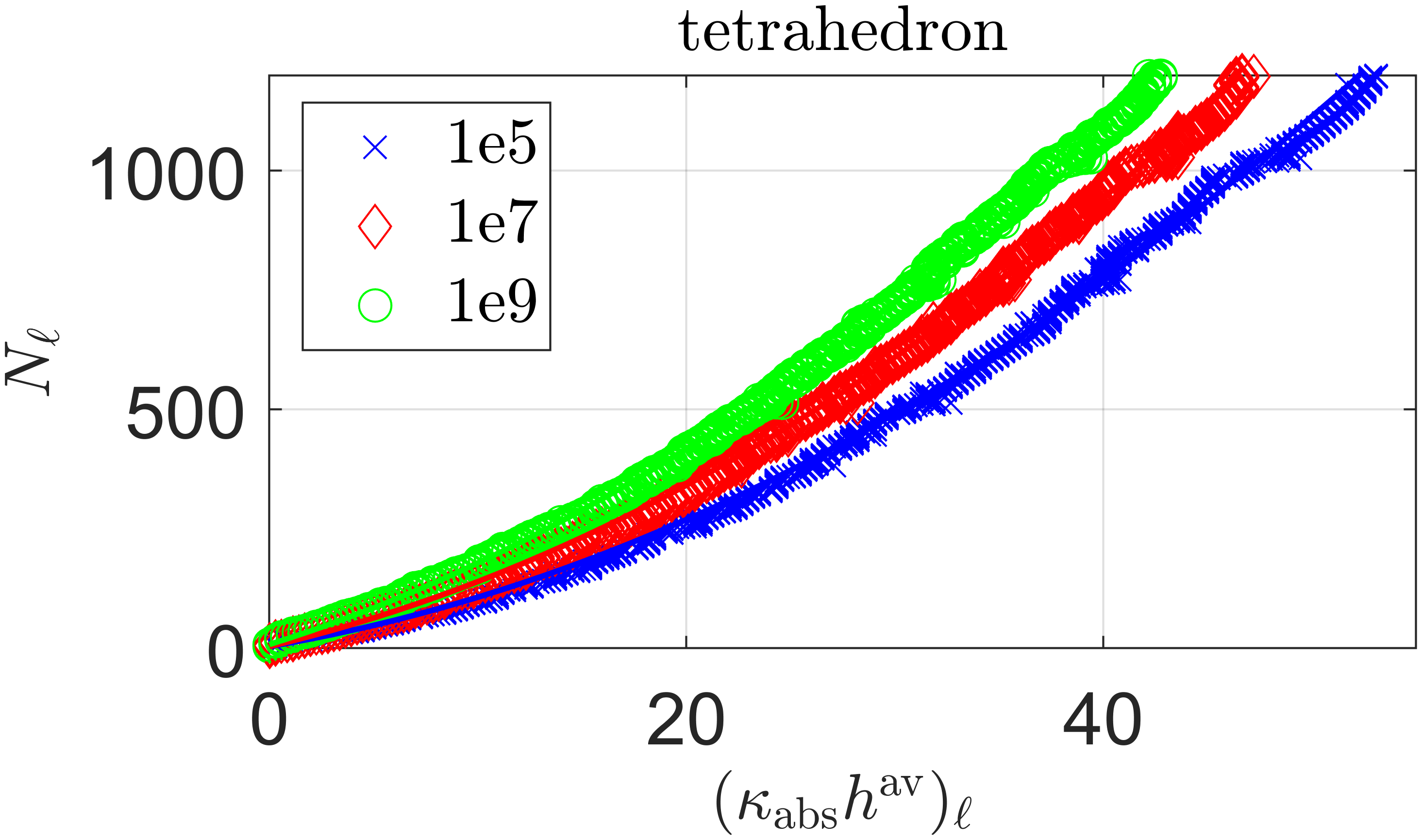
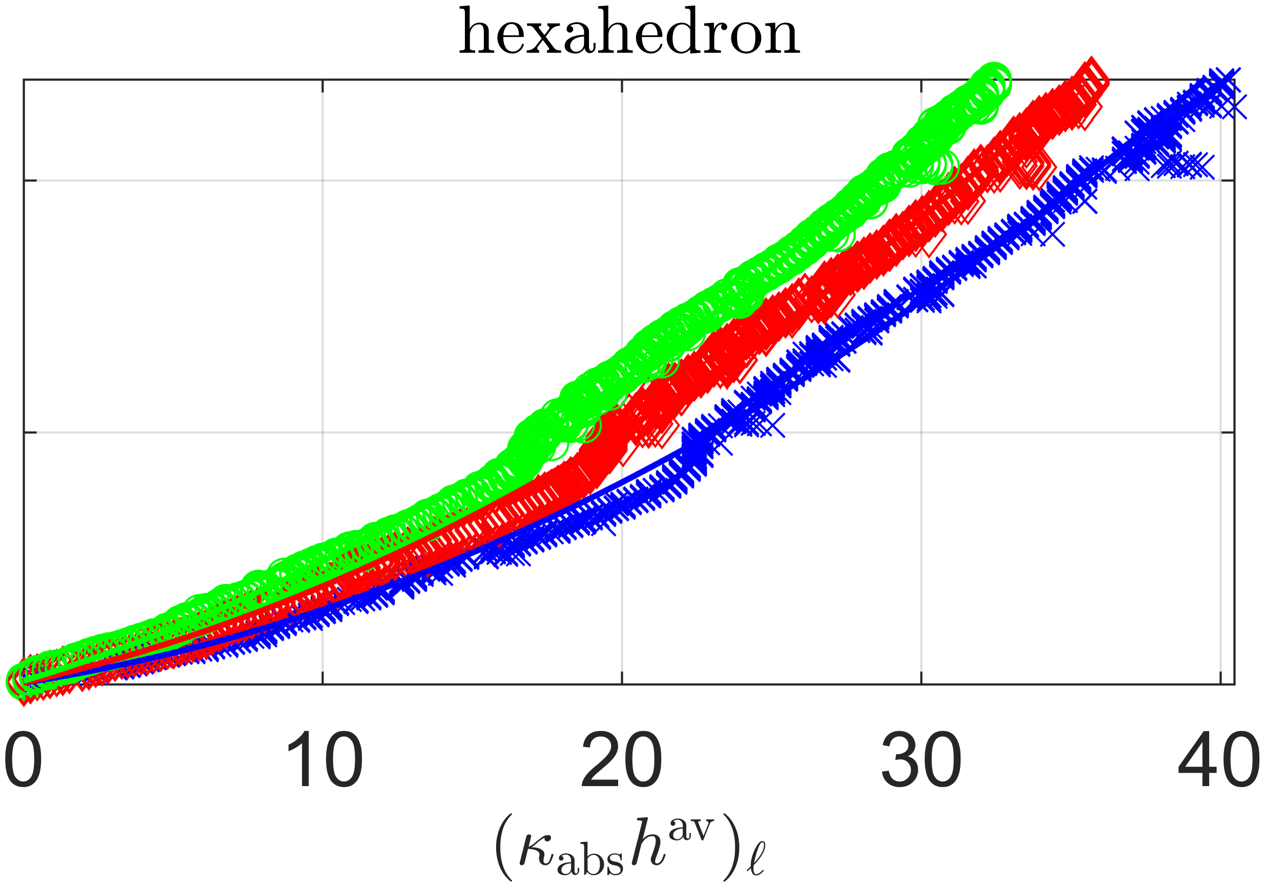
Figure 19: The number of basis functions $N_{\ell}$ as a function of $(\kappa_{\mathrm{abs}}h^{\mathrm{av}})_{\ell}$ when the basis dimension is chosen by constraining the maximum condition number of $D_{\ell}$.

Table 4: Parameters for the basis polynomials (see (16)).

		tetrahedron			hexahedron			wedge
max(cond($D_{k}$))	$a$	$b$	$c$	$a$	$b$	$c$	$a$	$b$	$c$
1e5	0.2972	7.3336	4.0000	0.5365	9.1369	4.0000	0.3752	9.0041	4.0000
1e7	0.3305	10.2707	4.0000	0.5803	13.3338	4.0000	0.4325	12.2717	4.0000
1e9	0.3430	13.6221	8.1296	0.5967	17.7977	7.7490	0.4704	15.6097	9.9414

Appendix B Comparison to edge elements

There are many ways to solve the scattering example problems in this paper. To provide a comparison to a more familiar method, we now use ParMax and the edge finite element method to compute scattering from a dielectric sphere. The exact Mie series is used to assess accuracy at several frequencies.

We have used the open source Netgen/NGSolve finite element package [21]. This is a library of highly optimised C++ function supporting multithreading that can be used via a Python interface (called NGSpy). It includes the Netgen mesh generator. We use $p$th order Nédélec edge elements of full polynomial degree on a tetrahedral mesh with a rectilinear PML and an outer impedance boundary condition. A direct sparse matrix solver supplied with NGSpy was used to solve the linear system. This limited the overall size of the problem we could solve to approximately 1.2 million degrees of freedom.

In order to make the application of the FEM possible, the computational domain described in Section 4.3 is not used here. Instead, the computational domain is the cube $[-1-(1+d_{\mathrm{pml}})\lambda_{0},1+(1+d_{\mathrm{pml}})\lambda_{0}]^{3}$. A PML of relative width $d_{\mathrm{pml}}=0.3$ with FEM and $d_{\mathrm{pml}}=1$ with ParMax is added within this cube. For the FEM, we requested NGSpy to use the mesh size $\lambda_{0}(2p+1)/(4\pi)$ outside the scatterer and increased $p$ gradually from $p=3$ to $p=8$ as $\lambda_{0}$ decreased to maintain an accuracy of roughly 1% in the computed RCS. Inside the scatterer the mesh size is reduced by a factor of 0.4.

Figure 20: Comparison results between NGSpy and ParMax.

The computations were run on an Intel Xeon Gold 6138 CPU 2.00GHz with 20 cores, each having two threads per core, and 394GB of memory. Since NGSpy ran multithreaded computations, we ran ParMax with MPI and 20 cores. Elapsed time is reported for NGSpy and ParMax, including assembly, matrix factorization, solving, and computation of the far-field pattern. The error reported is the relative percentage error in the RCS compared to the Mie solution. The results are shown in Fig. 20.

Figure 20 (top) shows that the relative L2-error remains comparable between NGSpy and ParMax across the entire frequency spectrum used here. As illustrated in Fig. 20 (middle), the number of degrees of freedom required by NGSpy increases more rapidly than that for ParMax. Likewise, the comparison in Fig. 20 (bottom) reveals that the CPU-time required by NGSpy increases more significantly compared to ParMax. This could perhaps be ameliorated using an auxiliary space preconditioned iterative scheme [12] rather than a direct factorization, but this is not available to us in NGSpy.

References

- [1] CSC – IT Center for Science Ltd, Computing environments. https://docs.csc.fi/computing/available-systems/. Accessed: Aug. 1, 2023.
- [2] Z. Badics. Trefftz-Discontinuous Galerkin and finite element multi-solver technique for modeling time-harmonic EM problems with high-conductivity regions. IEEE Trans. on Magnetics., 50(2):401–404, 2014.
- [3] J.-P. Bérenger. A Perfectly Matched Layer for the absorption of electromagnetic waves. J. Comput. Phys., 114(2):185–200, 1994.
- [4] A. Buffa and P. Monk. Error estimates for the Ultra Weak Variational Formulation of the Helmholtz equation. ESAIM: Mathematical Modeling and Numerical Analysis, 42:925–40, 2008.
- [5] O. Cessenat. Application d’une nouvelle formulation variationnelle aux équations d’ondes harmoniques. Problèmes de Helmholtz 2D et de Maxwell 3D. PhD thesis, Université Paris IX Dauphine, 1996.
- [6] O. Cessenat and B. Després. Using plane waves as base functions for solving time harmonic equations with the Ultra Weak Variational Formulation. J. Comput. Acoust., 11:227–38, 2003.
- [7] C. Gittelson, R. Hiptmair, and I. Perugia. Plane wave discontinuous Galerkin methods. ESAIM: Mathematical Modeling and Numerical Analysis, 43:297–331, 2009.
- [8] C. Hafner. MMP calculations of guided waves. IEEE Trans. On Magn., 21, 1985.
- [9] D. Hardin, T. Michaels, and E. Saff. A comparison of popular point configurations on . Dolomites Research Notes on Approximation, 9:16–19, 2016.
- [10] R. Hiptmair, A. Moiola, and I. Perugia. Stability results for the time-harmonic Maxwell equations with impedance boundary conditions. Math. Meth. Appl. Sci., 21:2263–87, 2011.
- [11] R. Hiptmair, A. Moiola, and I. Perugia. Error analysis of Trefftz-discontinuous Galerkin methods for the time-harmonic Maxwell equations. Math. Comput., 82:247–268, 2013.
- [12] R. Hiptmair and J. Xu. Nodal auxiliary space preconditioning in and spaces. SIAM J. Numer. Anal., 45:2483–2509, 2007.
- [13] T. Huttunen, M. Malinen, and P. Monk. Solving Maxwell’s equations using the ultra weak variational formulation. J. Comput. Phys., 223:731–758, 2007.
- [14] L. Imbert-Gérard and G. Sylvand. A roadmap for Generalized Plane Waves and their interpolation properties. Numer. Math., 149:87–137, 2021.
- [15] J. Jin, J. Volakis, C. Yu, and A. Woo. Modeling of resistive sheets in finite element solutions. IEEE Trans. Antennas Propag., 40:727–731, 1992.
- [16] G. Karypis and V. Kumar. A fast and high quality multilevel scheme for partitioning irregular graphs. SIAM J. Sci. Comput., 20(1):359–392, 1998.
- [17] C. Lehrenfeld and P. Stocker. Embedded Trefftz discontinuous Galerkin methods. Int. J. Numer. Methods Eng., 124(17):3637–3661, 2023.
- [18] R. H. MacPhie and K.-L. Wu. A plane wave expansion of spherical wave functions for modal analysis of guided wave structures and scatterers. IEEE Trans. Antennas Propag., 51:2801–2805, 2003.
- [19] P. Monk. Finite Element Methods for Maxwell’s Equations. Oxford University Press, Oxford, 2003.
- [20] S. Pernet, M. Sirdey, and S. Tordeux. Ultra-weak variational formulation for heterogeneous Maxwell problem in the context of high performance computing. Available as https://hal.science/hal-03642116 from the Hal preprint server., 2022.
- [21] J. Schöberl. Netgen/NGSolve. Downloaded from https://ngsolve.org, 2023.
- [22] T. Senior. Combined resistive and conductive sheets. IEEE Trans. Antennas Propag., AP-33:577–579, 1985.
- [23] P. Stocker. NGSTrefftz: Add-on to NGSolve for Trefftz methods. J. Open Source Soft., 7, 2022. Art. No. 4135.
- [24] E. Trefftz. Ein gegenstück zum Ritz’schen verfahren. In Proc. 2nd Int. Congr. Appl. Mech., pages 131–137, Zurich, 1926.