Resilient source seeking with robot swarms

Abstract

We present a solution for locating the source, or maximum, of an unknown scalar field using a swarm of mobile robots. Unlike relying on the traditional gradient information, the swarm determines an ascending direction to approach the source with arbitrary precision. The ascending direction is calculated from measurements of the field strength at the robot locations and their relative positions concerning the centroid. Rather than focusing on individual robots, we focus the analysis on the density of robots per unit area to guarantee a more resilient swarm, i.e., the functionality remains even if individuals go missing or are misplaced during the mission. We reinforce the robustness of the algorithm by providing sufficient conditions for the swarm shape so that the ascending direction is almost parallel to the gradient. The swarm can respond to an unexpected environment by morphing its shape and exploiting the existence of multiple ascending directions. Finally, we validate our approach numerically with hundreds of robots. The fact that a large number of robots always calculate an ascending direction compensates for the loss of individuals and mitigates issues arising from the actuator and sensor noises.

I Introduction

I-A Aim and objectives

The source seeking of a scalar field is regarded as one of the fundamental problems in swarm robotics due to its enormous potential for contemporary challenges [1, 2]. Indeed, the ability to detect and surround sources of chemicals, pollution, and radio signals effectively with robot swarms will enable persistent missions in vast areas for environmental monitoring, search & rescue, and precision agriculture operations [3, 4, 5, 6, 7].

Robot swarms are among the most promising multi-robot systems because of their high-resilience potential, i.e., to preserve functionality against unexpected adverse conditions and unknown, possibly unmodeled, disturbances. In this regard, we aim to a source-seeking algorithm for robot swarms with guarantees where the robots reach the source even if (disposable) individuals go missing during the mission. The algorithm guarantees an ascending direction rather than the gradient in order to guide the centroid of the robot swarm to the source, i.e., all the individual robots track such a direction. Its calculation does not require a specific formation; in fact, by morphing its shape, the swarm adapts to the environment, and missing robots are not an issue since the resultant formation is still valid. Calculating the ascending direction requires the robots to measure the strength of the scalar field at their current positions and then share this information with a computing-unit robot. The computing unit does not have any specific requirements, and, in fact, redundant computing units can be employed to enhance the robustness of the swarm. Additionally, the robots must be aware of their centroid. Due to space constraints, the objective of this paper is to determine the properties of the proposed ascending direction. In an upcoming journal version, we will show a more effective decentralization of all calculations and explore the compatibility of distributed formation control, distributed centroid estimation, and the unicycle dynamics with constants speeds with our source-seeking algorithm.

I-B Literature review

The following aims to help readers to assess pros and cons of different algorithms, considering that robot systems are tailored to specific requirements, e.g., robot dynamics, traveled distance, or communication topologies.

The widely used approaches focus on estimating the gradient and the Hessian of an unknown scalar field. In works like [8, 9], the estimation of the gradient occurs in a distributed manner, where each robot calculates the gradients at their positions. A common direction for the team is achieved through a distance-based formation controller that maintains the cohesion of the robot swarm. It is worth noting that this method fails when a subset of neighboring robots adopt a degenerate shape, like a line in a 2D plane. Alternatively, in studies like [10, 11], the gradient and Hessian are estimated at the centroid of a circular formation consisting of unicycles. However, it is relatively rigid due to its mandatory circular formation. Such a formation of unicycles is also present in [12], although robots are not required to measure relative positions but rather relative headings. In contrast to our algorithm, which calculates an ascending direction instead of the gradient, our robot team enjoys greater flexibility concerning formation shapes while still offering formal guarantees for reaching the source.

Extremum seeking is another extensively employed technique, as discussed in [13, 14]. In these studies, robots, which could potentially be just one, with nonholonomic dynamics execute periodic movements to facilitate a gradient estimation. However, when multiple robots are involved, there is a necessity for the exchange of estimated parameters. Furthermore, the eventual trajectories of the robots are often characterized by long and intricate paths with abrupt turns. In contrast, our algorithm generates smoother trajectories in, albeit requiring more than two robots.

All the algorithms above require communication among robots sharing the strength of the scalar field. Nonetheless, the authors in [15] offer an elegant solution involving the principal component analysis of the field that requires no sharing of the field strength. However, the centroid of the swarm is still necessary. It is worth noting that the initial positions of the robots determine the (time-varying) formation during the mission, and it is not under control. In comparison, although our algorithm requires the communication of the field strength among the robots, it is compatible with formation control laws that make the trajectory of the robots more predictable.

I-C Organization

The article is organized as follows. In Section II, we introduce notations and assumptions on the considered scalar field, and we formally state our source-seeking problem. We continue in Section III on how to calculate an ascending direction and analyze its sensitivity concerning the swarm and the observability of the gradient. In Section IV, we analyze the usage of the ascending direction with robots modeled as single integrators. We validate our theoretical findings in Section V involving hundreds of robots. Finally, we end this article in Section VI with conclusions and upcoming results.

II Preliminaries and problem formulation

Consider a team of $N\in\mathbb{N}$, with $N>2$ robots, where the position of the $i$-th robot in the Cartesian space is represented by $p_{i}\in\mathbb{R}^{m}$, where $m\in\{2,3\}$, $i\in\{1,\dots,N\}$. We define $p\in\mathbb{R}^{mN}$ as the stacked vector of the positions of all robots in the team. We will focus on the single integrator dynamics, i.e., the robot $i$ is modeled by

$$\dot{p}_{i}=u_{i},$$ (1)

where $u_{i}\in\mathbb{R}^{m}$ is the guiding velocity as control action. We define the centroid of the swarm as $p_{c}:=\frac{1}{N}\sum_{i=1}^{N}p_{i}$; therefore, we can write $p_{i}=p_{c}+x_{i}$, where $x_{i}\in\mathbb{R}^{m}$ for all $i\in\{1,\dots,N\}$ describes how robots are spread around their centroid as it is shown in Figure 1.

Definition 1.

The deployment of a swarm is defined as the stacked vector $x:=\begin{bmatrix}x_{1}^{T},\dots,x_{N}^{T}\end{bmatrix}^{T}\in\mathbb{R}^{mN}$. We say that a deployment is non-degenerate if the elements in $x$ span $\mathbb{R}^{m}$.

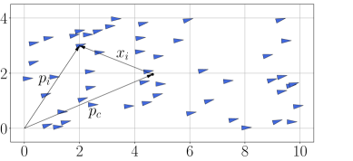
Figure 1: Deployment $x$ of a robot swarm with centroid at $p_{c}$.

Therefore, a necessary condition for a non-degenerate deployment is that $N>m$. The strength of a signal throughout the space can be described by a scalar field.

Definition 2.

A signal is a scalar field $\sigma:\mathbb{R}^{m}\to\mathbb{R}^{+}$ which is $C^{2}$ and all its partial derivatives up to second order are bounded globally. Also, $\sigma$ has only one maximum at $p_{\sigma}\in\mathbb{R}^{m}$, i.e., the source of the signal, and its gradient at $a\in\mathbb{R}^{m}$ satisfies $\nabla\sigma(a)\neq 0\iff a\neq p_{\sigma}$ and $\lim_{|a|\to\infty}\sigma(a)=0$.

Our definition of signal fits plenty of models in our physical world; e.g., Gaussian distributions and the power law $\frac{1}{r^{2}}$, smoothly modified at the origin to avoid singularities.

In this paper, the gradient is defined as a column vector, i.e., $\nabla\sigma(\cdot)\in\mathbb{R}^{m}$, and according to our definition of a signal:

$$\|\nabla\sigma(a)\|\leq K\quad\text{and}\quad\|H_{\sigma}(a)\|\leq 2M,\,\forall a\in\mathbb{R}^{m},$$ (2)

where $K,M\in\mathbb{R}^{+}$, and $H_{\sigma}$ is the Hessian of the scalar field $\sigma$, i.e., $H_{\sigma}(a)\in\mathbb{R}^{m\times m}$; thus, from the Taylor series expansion of $\sigma$ at $a\in\mathbb{R}^{m}$ [16, Theorem 5.15], it follows that

$$|\sigma(a)-\sigma(b)-\nabla\sigma(a)^{T}(a-b)|\leq M\|a-b\|^{2},\,\forall b\in\mathbb{R}^{m}.$$ (3)

Now we are ready to define the source-seeking problem.

Problem 1 (source seeking).

Given an unknown signal $\sigma$ and a constant $\epsilon\in\mathbb{R}^{+}$, find control actions for (1) such that $\|p_{c}(t)-p_{\sigma}\|<\epsilon,\forall t\geq T$ for some finite time $T\in\mathbb{R}^{+}$, where $p_{c}$ is the centroid of the swarm and $p_{\sigma}$ is the source of the signal.

III The ascending direction.

The authors in [10] show that the following expression for a circular formation of $N\geq 3$ robots that are equally angle-spaced

$$\hat{\nabla}\sigma(p_{c}):=\frac{2}{ND^{2}}\sum_{i=1}^{N}\sigma(p_{i})(p_{i}-p_{c}),$$ (4)

is an estimation of the gradient at the center $p_{c}$ of the circumference with radius $D$. However, it is unclear how well (4) approximates the gradient for any generic deployment other than the circle, or its sensitivity to misplaced robots. In fact, without apparently major changes, the expression (4) can be extended significantly by admitting any generic deployment $x$, i.e., we will prove that the vector

$$L_{\sigma}(p_{c},x) :=\frac{1}{ND^{2}}\sum_{i=1}^{N}\sigma(p_{i})(p_{i}-p_{c})$$

$$=\frac{1}{ND^{2}}\sum_{i=1}^{N}\sigma(p_{c}+x_{i})x_{i},$$ (5)

is an ascending direction at $p_{c}$ for some mild conditions, where now $D=\operatorname{max}_{1\leq i\leq N}{\|x_{i}\|}$. We note that $L_{\sigma}$ is calculated by the computing unit. We remark that (5), unlike (4), is a function of a generic deployment $x$, and that the ascending direction is not necessarily parallel to the gradient. We will see that such a property is an advantage to maneuver the swarm by just morphing $x$, or to guarantee an ascending direction in the case of misplaced robots.

Let us approximate $\sigma(p_{c}+x_{i})$ in (5) to a two-term Taylor series for small $\|x_{i}\|$, i.e., $\sigma(p_{c}+x_{i})\approx\sigma(p_{c})+\nabla\sigma(p_{c})^{T}x_{i}$, so that $L_{\sigma}(p_{c},x)\approx L_{\sigma}^{0}(p_{c},x)+L_{\sigma}^{1}(p_{c},x)$, where $L^{0}_{\sigma}(p_{c},x)=\frac{1}{ND^{2}}\sum_{i=1}^{N}\sigma(p_{c})x_{i}=0$ since $\sum_{i=1}^{N}x_{i}=0$, and

$$L^{1}_{\sigma}(p_{c},x)=\frac{1}{ND^{2}}\sum_{i=1}^{N}\left(\nabla\sigma(p_{c})^{T}x_{i}\right)x_{i}.$$ (6)

Although the important property of $L^{1}_{\sigma}$ is its direction, the factor $\frac{1}{ND^{2}}$ makes $L^{1}_{\sigma}$ have the same physical units as the gradient. The direction of the vector $L^{1}_{\sigma}$ is interesting because, if $x$ is non-degenerate, then it is an always-ascending direction, in the sense that no more conditions are necessary, towards the source $p_{\sigma}$ at the centroid $p_{c}$.

Lemma 1.

If the deployment $x$ is non-degenerate and $p_{c}\neq p_{\sigma}$, then $L^{1}_{\sigma}(p_{c},x)$ is an always-ascending direction at $p_{c}$ towards the maximum $p_{\sigma}$ of the scalar field $\sigma$.

Proof.

If $L^{1}_{\sigma}$ is an always-ascending direction, then it needs to satisfy $\nabla\sigma(p_{c})^{T}L^{1}_{\sigma}(p_{c},x)>0$, which is true since

$$\nabla\sigma(p_{c})^{T}L^{1}_{\sigma}(p_{c},x)=\frac{1}{ND^{2}}\sum_{i=1}^{N}|\nabla\sigma(p_{c})^{T}x_{i}|^{2}$$

is positive if the deployment $x$ spans $\mathbb{R}^{m}$ and $p_{c}\neq p_{\sigma}$. ∎

Lemma 1 motivates us to analyze how fast $L^{1}_{\sigma}$ (6) diverges from $L_{\sigma}$ (5), the actual computed direction, concerning $\|x\|$.

Lemma 2.

For a signal $\sigma$, a conservative divergence between $L^{1}_{\sigma}(p_{c},x)$ and $L_{\sigma}(p_{c},x)$ depends linearly on $D$, i.e.,

$$\|L_{\sigma}(p_{c},x)-L^{1}_{\sigma}(p_{c},x)\|\leq MD,$$

where $M$ is the upper bound in (2).

Proof.

From (3), (5) and (6), then it follows that

$\displaystyle\leq\frac{1}{ND^{2}}\sum_{i=1}^{N}M\|x_{i}\|^{3}\leq MD.$ ∎

Remark 1.

We have now a clear strategy: how to design deployments $x$ such that $L_{\sigma}^{1}$ is (almost-)parallel to the gradient $\nabla\sigma$; hence, the (potential) deviation of $L_{\sigma}$ from $L_{\sigma}^{1}$ is still admissible to guarantee that $L_{\sigma}$ is an ascending direction. ∎

Indeed, if $D$ is small enough, then it is certain that $L_{\sigma}$ is an ascending direction like $L_{\sigma}^{1}$. However, what is a small $D$ for generic signals and deployments? Let us define $E:=L_{\sigma}-L_{\sigma}^{1}$. Then we have $\nabla\sigma(p_{c})^{T}L_{\sigma}=\nabla\sigma(p_{c})^{T}(L_{\sigma}^{1}+E)$, and let us consider a compact set $\mathcal{S}\subset\mathbb{R}^{m}$ with $p_{\sigma}\notin\mathcal{S}$. By the definition of $\sigma$ and its bounded gradient, we know that $\nabla\sigma(p_{c})^{T}L_{\sigma}^{1}$ has a minimum $F_{\mathcal{S}}(x)$ that depends on the chosen deployment $x$ and it is positive if $x$ is non-degenerate, for all $p_{c}\in\mathcal{S}$. Therefore, we have $\nabla\sigma(p_{c})^{T}L_{\sigma}\geq F_{\mathcal{S}}(x)-K_{\mathcal{S}}^{\text{max}}M_{\mathcal{S}}^{\text{max}}D$, where $K_{\mathcal{S}}^{\text{max}}$ and $M_{\mathcal{S}}^{\text{max}}$ are the maximum norms of the signal’s gradient and Hessian in $\mathcal{S}$, respectively; thus, if

$$F_{\mathcal{S}}(x)-K_{\mathcal{S}}^{\text{max}}M_{\mathcal{S}}D>0,$$ (7)

then $L_{\sigma}$ is an ascending direction in $\mathcal{S}$. Finding the minimum $F_{\mathcal{S}}(x)$ numerically can be an arduous task, so we can conservatively bound it using the following result.

Lemma 3.

If the deployment $x$ is non-degenerate, then there exists $C(x)>0$ such that

Proof.

First, we see that the trivial case $\nabla\sigma(p_{c})=0$ satisfies the claim. In any other case, we know from Lemma 1 that $\nabla\sigma(p_{c})^{T}L^{1}_{\sigma}(p_{c},x)=\frac{1}{ND^{2}}\sum_{i=1}^{N}|\nabla\sigma(p_{c})^{T}x_{i}|^{2}=\frac{1}{ND^{2}}\nabla\sigma(p_{c})^{T}P(x)\nabla\sigma(p_{c})>0$ for the positive definite matrix $P(x)=\sum_{i=1}^{N}x_{i}x_{i}^{T}$ since $x$ is non-degenerate. Therefore,

$$\frac{\lambda_{\text{min}}\{P(x)\}}{ND^{2}}\|\nabla\sigma\|^{2}\leq\nabla\sigma^{T}L^{1}_{\sigma}\leq\frac{\lambda_{\text{max}}\{P(x)\}}{ND^{2}}\|\nabla\sigma\|^{2},$$

where $\lambda_{\text{\{min,max\}}}\{P(x)\}$ are the minimum and maximum eigenvalues of $P(x)$, respectively. We choose $C(x)=\max\{\frac{\lambda_{\text{max}}\{P(x)\}}{ND^{2}},\frac{ND^{2}}{\lambda_{\text{min}}\{P(x)\}}\}$. ∎

Later, we will see that $\lambda_{\text{min}}\{P(x)\}=\lambda_{\text{max}}\{P(x)\}$ for regular polygons/polyhedron deployments. Now we are ready to give an easier-to-check condition than (7).

Proposition 1.

Let $\mathcal{S}$ be a compact set with $p_{\sigma}\notin\mathcal{S}$. Then if

$$\lambda_{\text{min}}\{P(x)\}K^{\text{min}}_{\mathcal{S}}-NM_{\mathcal{S}}D^{3}>0,$$

for $x\in\mathcal{S}$, where $K^{\text{min}}_{\mathcal{S}}$ is the minimum norm of the gradient in the compact set $\mathcal{S}$, $P(x)=\sum_{i=1}^{N}x_{i}x_{i}^{T}$, then (5) is an ascending direction at $p_{c}\in\mathcal{S}$.

Proof.

Since Lemma 3 lower bounds $F_{\mathcal{S}}(x)$ in (7) we have

$$\nabla\sigma(p_{c})^{T}L_{\sigma} =\nabla\sigma(p_{c})^{T}L^{1}_{\sigma}+\nabla\sigma(p_{c})^{T}E$$

$$=\frac{1}{ND^{2}}\nabla\sigma(p_{c})^{T}P(x)\nabla\sigma(p_{c})+\nabla\sigma(p_{c})^{T}E$$

$$\geq\frac{\lambda_{\text{min}}\{P(x)\}}{ND^{2}}\|\nabla\sigma(p_{c})\|^{2}+\nabla\sigma(p_{c})^{T}E,$$

and to asses that $L_{\sigma}(p_{c})$ with $p_{c}\in\mathcal{S}$ is an ascending direction, we need to satisfy $\frac{\lambda_{\text{min}}\{P(x)\}}{ND^{2}}\|\nabla\sigma(p_{c})\|^{2}-\|\nabla\sigma(p_{c})\|M_{\mathcal{S}}D>0$ or equivalently $\lambda_{\text{min}}\{P(x)\}K^{\text{min}}_{\mathcal{S}}-NM_{\mathcal{S}}D^{3}>0$. ∎

The dependency on the number of robots $N$ is a bit misleading in the condition of Proposition 1 since $P(x)=\sum_{i=1}^{N}x_{i}x_{i}^{T}$ in the first term also depends on $N$. We can say something similar on the dependency on $D^{3}$ since $P(x)$ counterbalances $D^{2}$ because it consists of the elements $x_{i}x_{i}^{T}$, making the effective dependency of Proposition 1 on $D$ linear rather than cubic, matching the result of Lemma 2.

While the signal $\sigma$ is unknown, we can always engineer $D$ depending on the expected scenarios. For example, in the scenario of contaminant leakage, scientists can provide the expected values of $M_{\mathcal{S}}^{\text{max}},K_{\mathcal{S}}^{\text{max}}$, and $K_{\mathcal{S}}^{\text{min}}$ in the patrolling area $\mathcal{S}$ for the minimum/maximum contamination thresholds where the robot team needs to react reliably. We also note that designing $L^{1}_{\sigma}$ to be parallel to the gradient $\nabla\sigma$ makes the scalar product $\nabla\sigma^{T}L_{\sigma}>0$ more robust concerning $D$ since it makes admissible a larger deviation of $L_{\sigma}$ from $L^{1}_{\sigma}$, e.g., misplaced robots from a reference deployment $x$.

We organize the rest of the analysis in the following way. Firstly, we analyze the 4-robot case forming a rectangle. Secondly, we focus on regular polygons and affine transformations, i.e., the morphing of $x$, to check the sensitivity of the ascending direction. Thirdly, in a clear exploitation of superposition, we analyze the deployment of $N\to\infty$ robots following a robot density distribution within a shape or area.

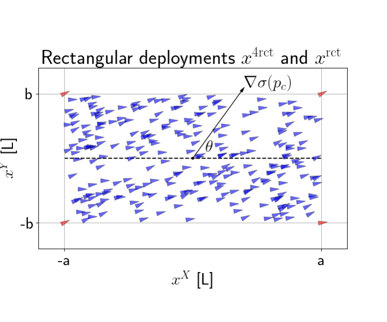
Figure 2: The 4-robot rectangular deployment $x^{\text{4rct}}$ are at the corners of the rectangle in red color. The $250$ robots in blue color belong to the deployment $x^{\text{rct}}$ and they are spread uniformly within the rectangle. The gradient $\nabla\sigma(p_{c})$ is arbitrary and forms an angle $\theta$ with the horizontal axis of the deployment.

Consider four robots at the corners of a rectangle as deployment $x^{4\text{rct}}$, and assume that the long side of the rectangle is parallel to the horizontal axis so that the gradient $\nabla\sigma(p_{c})=\|\nabla\sigma(p_{c})\|\left[\begin{smallmatrix}\cos(\theta)&\sin(\theta)\end{smallmatrix}\right]^{T}$ has an arbitrary norm and angle as depicted in Figure 2. Then, the always-ascending direction $L^{1}_{\sigma}$ can be written as

where the superscripts $X$ and $Y$ denote the horizontal and vertical coordinates of $x_{i}$ respectively. Therefore, for the deployment $x^{4\text{rct}}$ we have that

(9)

where we can observe that if $a$ or $b$ equals zero, then only the projection of $\nabla\sigma(p_{c})$ onto the line described by the degenerate $x$ in $L^{1}_{\sigma}(p_{c},x^{4\text{rct}})$ is observed. We can also see that for the square $a=b$, we have that $L^{1}_{\sigma}(p_{c},x^{4\text{rct}})=\frac{1}{2}\nabla\sigma(p_{c})$. In general, $L^{1}_{\sigma}(p_{c},x^{N\text{poly}})\propto\left[\begin{smallmatrix}\cos\theta&\sin\theta\end{smallmatrix}\right]^{T}$, i.e., it is parallel to $\nabla\sigma(p_{c})$, for any deployment $x^{N\text{poly}}$ forming a regular polygon or polyhedron as it is shown in the following technical result.

Lemma 4.

Consider the deployment $x^{N\text{poly}}$ forming a regular polygon or polyhedron, and $b\in\mathbb{R}^{m}$, then

$$\sum_{i=1}^{N}\left(b^{T}x_{i}\right)x_{i}\propto b.$$

Proof.

First, we have that $\sum_{i=1}^{N}\left(b^{T}x_{i}\right)x_{i}=\sum_{i=1}^{N}(x_{i}x_{i}^{T})b$; then, in order to be proportional to $b$, we need all the diagonal elements of the positive semi-definite matrix $P=\sum_{i=1}^{N}(x_{i}x_{i}^{T})$ be equal, and the non-diagonal to be zero. Since all the considered deployments lie on the $(m-1)$-sphere, then all the $\|x_{i}\|$ are equal. In addition, all the dihedral angles of the considered deployments are equal, then we can find XYZ axes where the set of all projections of the vertices $x_{i}$ on the planes XY, XZ, and YZ, exhibit an even symmetry; hence, $\sum_{i}^{N}(x_{i}^{X})^{2}=\sum_{i}^{N}(x_{i}^{Y})^{2}=\sum_{i}^{N}(x_{i}^{Z})^{2}$. Finally, a regular polygon has reflection symmetry for one axis of the same XY; hence, $\sum_{i}^{N}(x_{i}^{X})(x_{i}^{Y})=0$. This is also true for a regular polyhedron for the same planes XY, XZ, and YZ. ∎

A similar result has been shown in [10, 11] with their circular and spherical formations since regular polygons and polyhedra are inscribed in the circle and sphere. We now analyze the sensitivity of $L^{1}_{\sigma}(p_{c},x^{N\text{poly}})$ when the deployment is under an affine transformation, e.g., scaling, rotation, and shearing. The formal affine transformation is given by $(I_{N}\otimes A)x^{N\text{poly}}$ with $A\in\mathbb{R}^{m\times m}$ where $A$ admits the Singular Value Decomposition (SVD) $A=U\Sigma V^{T}$ describing a rotation, scaling, and another rotation.

Proposition 2.

Consider the deployment $x^{N\text{poly}}$ forming a regular polygon or polyhedron, and the SVD $A=U\Sigma V^{T}$, then

$$L^{1}_{\sigma}(p_{c},(I_{N}\otimes A)x^{N\text{poly}})\propto U\Sigma^{2}U^{T}r,$$

where $r\in\mathbb{R}^{m}$ is the unitary vector marking the direction of the gradient $\nabla\sigma(p_{c})$.

Proof.

Considering the change of coordinates $\tilde{r}=V\Sigma U^{T}r$

where we have applied Lemma 4. ∎

Note that $W=U\Sigma^{2}U^{T}$ is the unitary decomposition of a positive definite matrix, and $V$ is irrelevant since $\theta$ is arbitrary as it is shown in Lemma 4. Stretching the deployment $x^{N\text{poly}}$ results in $L_{\sigma}^{1}$ following the direction ${{}^{\xi}\Sigma^{2}}\,\,{{}^{\xi}\nabla\sigma(p_{c})}$, where $\xi$ denotes the stretching axes. Such a morphing maneuvers the swarm while it gets closer to the source.

Looking at the definition of $L_{\sigma}$ in (5), it is clear that we can apply the superposition of many, potentially infinite, deployments. Indeed, we can step to continuous deployments considering $N\to\infty$ within a specific area or volume. In such a case, the finite sum in (5) becomes an integral with a robot density function following the approximation of a definite integral with Riemann sums, and $ND^{2}$ in (5) becomes $A=\iiint_{\mathcal{A}}\rho(X,Y,Z)\mathrm{d}X\mathrm{d}Y\mathrm{d}Z$, where $\mathcal{A}$ is the corresponding surface/volume or perimeter of $x$, and $\rho:\mathbb{R}^{m}\to\mathbb{R}^{+}$ is a standard (robot) density function, e.g., equal everywhere for uniform distributions as it is shown in Figure 2 with $x^{rct}$.

For the sake of conciseness, let us focus on 2D for the following results, and for the sake of clarity with the notation, we will denote $x_{i}^{X}$ and $x_{i}^{Y}$ as simply $X$ and $Y$. Accordingly, for the case of a robot swarm following a density function $\rho(X,Y)$ of robots within a generic shape/surface $\mathcal{A}$, the always-ascending direction can be calculated as

Similar to the discrete case, e.g., see (9), it is enough to have $\iint_{\mathcal{A}}\rho(X,Y)XY\mathrm{d}X\mathrm{d}Y$ and $\iint_{\mathcal{A}}\rho(X,Y)(X^{2}-Y^{2})\mathrm{d}X\mathrm{d}Y$ equal to zero to have $L^{1}_{\sigma}$ parallel to the gradient.

Proposition 3.

Consider a signal $\sigma$, a continuous deployment $x$ with robot density function $\rho(X,Y)$ within a surface $\mathcal{A}$, and a Cartesian coordinate system $(X-Y)$ with origin at the centroid of the deployment $p_{c}$. The direction of $L_{\sigma}^{1}(p_{c},x)$ is parallel to the gradient $\nabla\sigma(p_{c})$ if $\rho(X,Y)$ and $\mathcal{A}$ hold the following symmetries:

1. The robot density function $\rho(X,Y)$ has reflection symmetry (even function) concerning at least one of the axes $(X-Y)$, e.g., $\rho(X,Y)=\rho(-X,Y)$.

2. The surface $\mathcal{A}$ has reflection symmetry concerning the same axes as in S0.

3. For each quadrant of $(X-Y)$, the robot density function $\rho(X,Y)$ has reflection symmetry concerning the bisector of the quadrant.

4. The surface $\mathcal{A}$ has reflection symmetry concerning the same axes as in S2.

Proof.

Without loss of generality, we assume that the reflection symmetry is on the $Y$ axis, and we assume symmetric integration limits for the horizontal axis as in Figure 3(a). First, if $\alpha(X)$ and $\beta(X)$ are both even functions as illustrated in Figure 3(a), we are going to show that

$$\scalebox{0.8}{\mbox{$\displaystyle\quad=\int_{-t_{\beta}}^{t_{\beta}}XF(X,\beta(X))\,\mathrm{d}X-\int_{-t_{\alpha}}^{t_{\alpha}}XF(X,\alpha(X))\,\mathrm{d}X=0$}},$$ (10)

where $F(X,Y)=\int\rho(X,Y)Y\;\mathrm{d}Y$. Given an arbitrary even function $f(X)$ and knowing that $\rho(X,Y)=\rho(-X,Y)$, we have that $F(X,Y)=F(-X,Y)$ and $F(X,Y)=F(X,f(X))=F(-X,f(-X))=F(X,-Y)$; therefore, both integrals in (10) are zero considering symmetries S{0,1}.

Next, we will divide $\mathcal{A}$ in four parts for each quadrant as it is shown in Figure 3(b), so that

$$\scalebox{0.8}{\mbox{$\displaystyle\iint_{\mathcal{A}}\rho(X,Y)(X^{2}-Y^{2})\;\mathrm{d}X\mathrm{d}Y=\sum_{i=1}^{4}\iint_{\mathcal{A}_{i}}\rho(X,Y)(X^{2}-Y^{2})\;\mathrm{d}X\mathrm{d}Y$}},$$

where $\mathcal{A}_{i}$ is the area of the quadrant $i\in\{1,2,3,4\}$. From the symmetry exhibited by $X^{2}-Y^{2}$ we propose the following change of variables $g(\epsilon,\psi)=(\psi+\epsilon,\psi-\epsilon)/\sqrt{2}$, which is equivalent to a rotation of $-\frac{\pi}{4}$ radians for the $(X-Y)$ axes. Since $\int_{A}f(x,y)=\int_{B}(f\circ g)|J_{g}|$, where $|J_{g}|=|\begin{bmatrix}\nabla g_{1}&\nabla g_{2}\end{bmatrix}^{T}|=\sqrt{2}$, we have

$$\scalebox{0.8}{\mbox{$\displaystyle=2\sqrt{2}\int_{-t_{i}}^{t_{i}}\int_{|\epsilon|}^{R_{i}(\epsilon)}\rho(\epsilon,\psi)\epsilon\psi\;d\epsilon d\psi=2\sqrt{2}\int_{-t_{i}}^{t_{i}}\epsilon\left[F(\epsilon,R_{i}(\epsilon))-F(\epsilon,|\epsilon|)\right]d\epsilon$}},$$

which is zero if $R_{i}(\epsilon)=R_{i}(-\epsilon)$ for all quadrants since $|\epsilon|$ is an even function. Such condition is satisfied if $\alpha(X)$ and $\beta(X)$ have reflection symmetry concerning the bisector of the two lower and upper quadrants respectively as illustrated in Figure 3(b); thus, symmetries S{2,3} are checked.∎

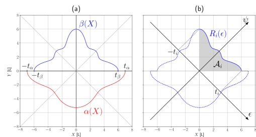
Figure 3: Illustration of the symmetries S{1,3} for the surface $\mathcal{A}$ on the left and right respectively, to design $L^{1}_{\sigma}(p_{c},x)$ parallel to the gradient $\nabla\sigma(p_{c})$.

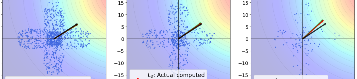
Figure 4: On the left, a swarm of $1000$ robots satisfying the symmetries $S\{0,1,2,3\}$ from Proposition 3. For the three figures, the black arrows are the gradient $\nabla\sigma$, the green arrows are $L^{1}_{\sigma}$, and the red arrows are the direction $L_{\sigma}$ computed by the robots. Arrows are normalized for representation porpuses as we focus only on their direction. As we get far from the continuum, with $500$ and $100$ robots on the middle and right figures, there is no guarantee that $L^{1}_{\sigma}$ is parallel to the gradient $\nabla\sigma$. However, in this example, $L_{\sigma}$ has almost the same direction as $L_{\sigma}^{1}$ despite a big $D$ concerning the level curves.

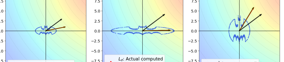
Figure 5: On the left, a swarm of $1000$ robots satisfying only the symmetries $S\{0,1\}$ from Proposition 3. The arrows have the same meaning as in Figure 4. The modification of the variances of $\rho(X,Y)$, e.g., by stretching the swarm shape, stretches $L^{1}_{\sigma}$ and $L_{\sigma}$ accordingly. In this example, the direction of $L_{\sigma}$ almost does not diverge from $L_{\sigma}^{1}$ despite a big $D$ concerning the level curves.

Indeed, not only uniform deployments $x^{\text{Upoly}}$ describing an area/volume of a regular polygon/polyhedron fit into Proposition 3, but a richer collection of deployments like the ones depicted in Figures 3 and 4. In fact, if only $S\{0,1\}$ are satisfied, concerning $\rho(X,Y)$, the variances $\text{VAR}_{\mathcal{A}}[X]\neq\text{VAR}_{\mathcal{A}}[Y]$ in general, so we have that

$$\scalebox{0.8}{\mbox{$\displaystyle L_{\sigma}^{1}(p_{c},x)=\frac{\|\nabla\sigma(p_{c})\|}{A}\begin{bmatrix}\text{VAR}_{\mathcal{A}}[X]\cos(\theta)\\ \text{VAR}_{\mathcal{A}}[Y]\sin(\theta)\\ \end{bmatrix}$}},$$

where the relation between variances maneuvers the swarm, while getting closer to the source, as it is shown in Figure 5.

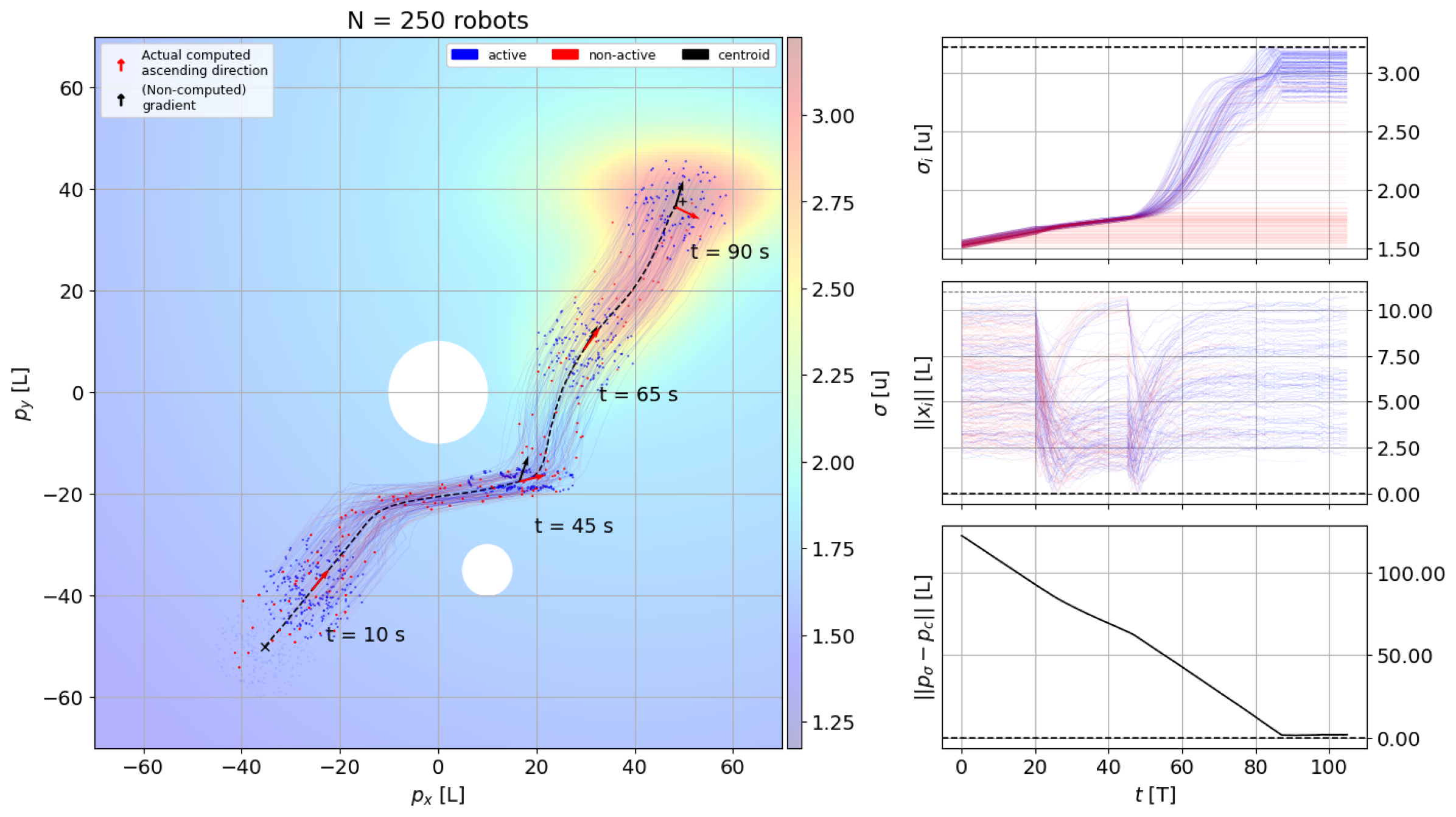
Figure 6: A robot swarm of $250$ individuals (blue dots) faces faulty actuators with noisy directions, and individuals stop working randomly (turned into red dots). The swarm maneuvers between two white obstacles by morphing its shape and reaches the signal source eventually, where $170$ robots were dead during the mission; nonetheless, the rest made it to the source, demonstrating the resiliency of the swarm. At the right side, from top to down: the readings of the signal by the robots, the distances from the robots to the swarm centroid, and the distance of the swarm centroid to the source.

IV Source seeking with single-integrator robots.

Focusing on robots with the single-integrator dynamics (1), the following theorem claims that $L_{\sigma}(p_{c}(t),x)$ can guide the centroid of the robot swarm effectively to the signal source.

Theorem 1.

Consider the signal $\sigma$ and a swarm of $N$ robots with the stacked positions $p(t)\in\mathbb{R}^{mN}$, where $m=\{2,3\}$, and a non-degenerate initial deployment $x^{*}$, then

$$\begin{cases}\dot{p}_{i}(t)&=\frac{L_{\sigma}(p_{c}(t),x(t))}{\|L_{\sigma}(p_{c}(t),x(t))\|}\\ p_{i}(0)&=p_{c}+x^{*}_{i},\quad p_{c}\neq p_{\sigma}\end{cases},\forall i\in\{1,\dots,N\},$$

is a solution to the source-seeking Problem 1.

Due to space limitation, we will present the technical proof in the upcoming journal version of this work. Nonetheless, the rational of the proof is as follows. For single integrators, the unit vector from $L_{\sigma}^{1}$ always points to a direction that, if followed, makes $p_{c}$ closer to the source $p_{\sigma}$, where such unit vector is not defined anymore. However, the centroid of the swarm would get arbitrarily close to $p_{\sigma}$ in finite time. The actual computed direction $L_{\sigma}$ approximates $L^{1}_{\sigma}$, and they diverge, in the worst case, linearly by $D$ with the bound $M$ of the Hessian field. How the centroid of the swarm would get arbitrarily close to the source follows the same rational as with $L_{\sigma}^{1}$, but such a distance depends now on the relation between $D$, $K_{\mathcal{S}}^{\text{min}}$, and $M_{\mathcal{S}}^{\text{max}}$ as stated in Proposition 1, where the smaller the $D$ the closer to the source; hence, solving the source-seeking problem as stated in Problem 1.

V Numerical simulation

Figure 6 shows a $250$ robot swarm seeking the source of the signal $\sigma(p)=(0.04\,\|p-40\left[\begin{smallmatrix}1\\ 1\end{smallmatrix}\right]\|-2)-\operatorname{exp}\{-0.9(p-40\left[\begin{smallmatrix}1\\ 1\end{smallmatrix}\right])^{T}\left[\begin{smallmatrix}\frac{1}{\sqrt{30}}&0\\ 0&1\end{smallmatrix}\right]\left[\begin{smallmatrix}1\\ 0\end{smallmatrix}\right]\}-\operatorname{exp}\{-0.45(p-40\left[\begin{smallmatrix}1\\ 1\end{smallmatrix}\right])^{T}\left[\begin{smallmatrix}1&1\\ -1&1\end{smallmatrix}\right]\left[\begin{smallmatrix}1&0\\ 0&\frac{1}{\sqrt{15}}\end{smallmatrix}\right]\left[\begin{smallmatrix}1&-1\\ 1&1\end{smallmatrix}\right]\left[\begin{smallmatrix}0\\ -2\end{smallmatrix}\right]\}$ by using the direction $L_{\sigma}$ (red arrow in Figure 6) in Theorem 1, i.e., robots move at an unitary speed. The swarm starts as a uniform circular cloud of radius $10$ length units. We show the resilience of the swarm by introducing the following three factors. Firstly, in order to show misplacements within the formation, we inject noise to the actuators, i.e., every $0.2$ time units the robots track the direction $L_{\sigma}$ with a random deviation within $\pm 10$ degrees. Secondly, at time $20$, the swarm maneuvers between two obstacles by morphing into the shape in Figure 5 since it stretches $L_{\sigma}$ horizontally. Thirdly, there is a random probability for individual robots to stop functioning. These dead robots are represented in red color, and only $80$ robots made it eventually to the source. At time $90$, the centroid swarm gets so close to the source that $L_{\sigma}$ becomes unreliable, i.e., the centroid entered the $\epsilon$-ball in Problem 1.

VI Conclusions and future work

Using a robot swarm that always calculates an ascending direction offsets individual losses and mitigates noise issues for the source-seeking problem, i.e., it adds resiliency. An upcoming journal version will show a more distributed computation of the ascending direction $L_{\sigma}$, including a fully distributed algorithm to estimate the centroid estimation, which is compatible with our source-seeking method. Finally, as anticipated in the attached video, we will analyze how our algorithm works with unicycles traveling at constant speeds.

References

- [1] G.-Z. Yang, J. Bellingham, P. E. Dupont, P. Fischer, L. Floridi, R. Full, N. Jacobstein, V. Kumar, M. McNutt, R. Merrifield et al., “The grand challenges of science robotics,” Science robotics, vol. 3, no. 14, p. eaar7650, 2018.
- [2] M. Brambilla, E. Ferrante, M. Birattari, and M. Dorigo, “Swarm robotics: a review from the swarm engineering perspective,” Swarm Intelligence, vol. 7, pp. 1–41, 2013.
- [3] P. Ogren, E. Fiorelli, and N. E. Leonard, “Cooperative control of mobile sensor networks: Adaptive gradient climbing in a distributed environment,” IEEE Transactions on Automatic control, vol. 49, no. 8, pp. 1292–1302, 2004.
- [4] V. Kumar, D. Rus, and S. Singh, “Robot and sensor networks for first responders,” IEEE Pervasive computing, vol. 3, no. 4, pp. 24–33, 2004.
- [5] K. McGuire, C. De Wagter, K. Tuyls, H. Kappen, and G. C. de Croon, “Minimal navigation solution for a swarm of tiny flying robots to explore an unknown environment,” Science Robotics, vol. 4, no. 35, p. eaaw9710, 2019.
- [6] W. Li, J. A. Farrell, S. Pang, and R. M. Arrieta, “Moth-inspired chemical plume tracing on an autonomous underwater vehicle,” IEEE Transactions on Robotics, vol. 22, no. 2, pp. 292–307, 2006.
- [7] J. N. Twigg, J. R. Fink, L. Y. Paul, and B. M. Sadler, “Rss gradient-assisted frontier exploration and radio source localization,” in 2012 IEEE International Conference on Robotics and Automation. IEEE, 2012, pp. 889–895.
- [8] E. Rosero and H. Werner, “Cooperative source seeking via gradient estimation and formation control,” in 2014 UKACC International Conference on Control (CONTROL). IEEE, 2014, pp. 634–639.
- [9] S. A. Barogh and H. Werner, “Cooperative source seeking with distance-based formation control and non-holonomic agents,” IFAC-PapersOnLine, vol. 50, no. 1, pp. 7917–7922, 2017.
- [10] L. Briñón-Arranz, L. Schenato, and A. Seuret, “Distributed source seeking via a circular formation of agents under communication constraints,” IEEE Transactions on Control of Network Systems, vol. 3, no. 2, pp. 104–115, 2015.
- [11] L. Briñón-Arranz, A. Renzaglia, and L. Schenato, “Multirobot symmetric formations for gradient and hessian estimation with application to source seeking,” IEEE Transactions on Robotics, vol. 35, no. 3, pp. 782–789, 2019.
- [12] R. Fabbiano, F. Garin, and C. Canudas-de Wit, “Distributed source seeking without global position information,” IEEE Transactions on Control of Network Systems, vol. 5, no. 1, pp. 228–238, 2016.
- [13] Z. Li, K. You, and S. Song, “Cooperative source seeking via networked multi-vehicle systems,” Automatica, vol. 115, p. 108853, 2020.
- [14] J. Cochran and M. Krstic, “Nonholonomic source seeking with tuning of angular velocity,” IEEE Transactions on Automatic Control, vol. 54, no. 4, pp. 717–731, 2009.
- [15] S. Al-Abri and F. Zhang, “A distributed active perception strategy for source seeking and level curve tracking,” IEEE Transactions on Automatic Control, vol. 67, no. 5, pp. 2459–2465, 2021.
- [16] W. Rudin, Principles of mathematical analysis, 3rd ed. McGraw-hill New York, 1976.