A Bayesian Nonparametric Method to Adjust for Unmeasured Confounding with Negative Controls

Abstract

Unmeasured confounding bias is among the largest threats to the validity of observational studies. Although sensitivity analyses and various study designs have been proposed to address this issue, they do not leverage the growing availability of auxiliary data accessible through open data platforms. Using negative controls has been introduced in the causal inference literature as a promising approach to account for unmeasured confounding bias. In this paper, we develop a Bayesian nonparametric method to estimate a causal exposure-response function (CERF). This estimation method effectively utilizes auxiliary information from negative control variables to adjust for unmeasured confounding completely. We model the CERF as a mixture of linear models. This strategy offers the dual advantage of capturing the potential nonlinear shape of CERFs, while still maintaining computational efficiency. Additionally, it leverages closed-form results that hold true under the linear model assumption. We assess the performance of our method through simulation studies. The results demonstrate the method’s ability to accurately recover the true shape of the CERF in the presence of unmeasured confounding. To showcase the practical utility of our approach, we apply it to adjust for a potential unmeasured confounder when evaluating the relationship between long-term exposure to ambient $PM_{2.5}$ and cardiovascular hospitalization rates among the elderly in the continental U.S. To ensure transparency and reproducibility, we implement our estimation procedure in open-source software and make our code publicly available.

1 Introduction

Proximal causal inference has been recently introduced in the causal inference literature as a promising approach to adjust for unmeasured confounding bias (Tchetgen et al., 2020; Miao et al., 2018). The key idea of proximal causal inference is to leverage auxiliary data that contain valuable information on unmeasured confounding mechanisms to estimate causal effects. Negative control exposure (NCE) and negative control outcome (NCO) variables are examples of such auxiliary information. An NCO variable $W$ is a variable known not to cause an outcome $Y$ and an NCE variable $Z$ is a variable known not to be causally affected by an exposure $X$ (Lipsitch et al., 2010). Under the assumption that the association between the NCE variable $Z$ and $Y$ is subject to the same unmeasured confounding mechanisms as the association between the exposure $X$ and $Y$, the detection of an association between $Z$ and $Y$ can signal the presence of an unmeasured confounder $U$ (Fig 1). Similarly, under the assumption that the association between $X$ and the NCO variable $W$ is subject to the same unmeasured confounding mechanism as between $X$ and the outcome $Y$, the detection of an association between $X$ and $W$ can signal the presence of an unmeasured confounder $U$ (Fig 1).

• W: negative control outcome

• Z: negative control exposure

• U: unmeasured confounder

• X: treatment or exposure

• Y: outcome

Figure 1: An illustration of negative control exposure and outcome.

Sometimes an accurate measurement of a confounder is unavailable, and often the best we can obtain is its proxies. These proxies also contain valuable information on the true confounders. They can be used as NCEs and NCOs in estimating causal effects in the presence of unmeasured confounding as well (Tchetgen et al., 2020).

Miao et al. (2018) and Cui et al. (2023) have demonstrated that, under certain conditions, the presence of a pair of NCE and NCO guarantees nonparametric identification of the average treatment effect (ATE). Since then, parametric, semi-parametric, nonparametric methods, and machine learning approaches have been developed to estimate causal effects using proxies and negative controls (NCs) (Cui et al., 2023; Shi et al., 2020a; Mastouri et al., 2023; Kompa et al., 2022; Ghassami et al., 2022). More specifically, in the context of binary and categorical treatments, Shi et al. (2020a) developed nonparametric methods that use NCs when $U$ is categorical. Cui et al. (2023) provided a general semiparametric theory for estimating ATE via a locally efficient influence function. Ghassami et al. (2022) framed the estimation of the nuisance functions in the influence function of Cui et al. (2023) as a minimax optimization problem and estimated this nuisance function using kernel methods without resorting to parametric models.

Continuous treatments and exposures are common, such as drug doses, air pollution levels, and heatwave intensity and duration. The causal effects of these continuous exposures are naturally described by causal exposure-response functions (CERFs). Several machine-learning approaches have been proposed for estimating CERFs using NCs. These approaches include 1) two-stage kernel ridge regression (Singh, 2023), 2) two-stage regression with adaptive basis derived from neural networks (Xu et al., 2021), 3) the maximum moment restriction method (Mastouri et al., 2023), 4) neural maximum moment restriction method (Kompa et al., 2022), and 5) the minimax learning estimation method (Kallus et al., 2022). Among this literature, Mastouri et al. (2023) and Kompa et al. (2022) implemented some of these methods to compare their performances. Although all the above methods have been shown consistency theoretically, when evaluated in the context of finite samples for continuous exposures, most of them do not perform well (see Figures S3 and S4 in Kompa et al., 2022). Furthermore, these machine-learning algorithms rarely provide uncertainty bounds for the estimates of CERFs.

In this paper, we propose a new approach to estimate the CERF of a continuous exposure ($X$) on a continuous outcome ($Y$) in the presence of unmeasured confounders ($U$). More specifically, we introduce the following contributions: 1) we develop a new Bayesian Nonparametric approach (BNP) for estimating the CERF that addresses unmeasured confounding by using NCs; 2) we quantify the uncertainty of our estimates in the form of credible intervals (CI); and 3) we provide R code on GitHub that is easy to apply to new problems.

In section 2, we review two key findings that inspire our method, one in proximal causal inference and the other in BNP mixture models literature. In section 3, we describe our method and innovation in detail. More specifically, we define our target parameter in section 3.1 and state our assumptions in section 3.2. Then, we introduce our nonparametric estimation approach in section 3.3. In section 4, we perform simulation studies to assess the performance of our method and demonstrate that it captures the true CERFs of various shapes under unmeasured confounding. In section 5, we apply our method to adjust for a potential unmeasured confounder when evaluating the relationship between long-term exposure to ambient $PM_{2.5}$ and cardiovascular hospitalizations across 5,362 zip code areas in the continental U.S. (Papadogeorgou and Dominici, 2020). We close by discussing our approach’s strengths, weaknesses, and future research areas. Our estimating procedure and simulation studies are implemented in R, available at https://github.com/NSAPH-Projects/BNP-For-Unmeasured-Confounding.

2 Technical Background

To estimate the CERF of a continuous exposure ($X$) on a continuous outcome ($Y$) in the presence of unmeasured confounders ($U$), we develop a new BNP approach that addresses unmeasured confounding using NCs. Before introducing our method, we review the conditions required for identifying the causal effect of $X$ on $Y$ under linear models and the setup of BNP mixture models. Our method is built upon these two methods but extends them to estimate the CERF nonparametrically.

Throughout the paper, we consider a sample of i.i.d. observations on the exposure $X$, outcome $Y$, NCE variable $Z$, and NCO variable $W$. We denote the unmeasured confounder by $U$ and let $Y(x)$ be the potential outcome one would observe if $X$ were set to the value $x$.

2.1 Identification of average treatment effect

Shi et al. (2020b) outlined the conditions for identifying the causal effect when the observed variables $(Y,X,Z,W)$ and the unobserved variable $U$ follow the linear models below:

$$\begin{array}[]{l@{}r}E[Y|X=x,U]=\beta_{Y0}+\beta_{YX}x+\beta_{YU}U,\\ E[W|U]=\beta_{W0}+\beta_{WU}U,\\ E[U|X=x,Z]=\beta_{U0}+\beta_{UX}x+\beta_{UZ}Z.\end{array}$$ (2.1)

More specifically, they considered the causal effect as a constant difference in the potential outcomes between two exposure levels and provided the following conditions for identifying the causal effect under linear models:

• C1. (Z is an NCE): $Y(x,z)=Y(x)$ and $Z\perp\!\!\!\perp Y(x)|U,X$;

• C2. (W is an NCO): $W(x,z)=W$ and $W\perp\!\!\!\perp X|U$;

• C3. (NCE and NCO are conditionally independent): $Z\perp\!\!\!\perp W|U$;

• C4 ($W$ and $Z$ are informative about $U$): $\beta_{WU}\neq 0$ and $\beta_{UZ}\neq 0$.

Figure 1 is one causal diagram among many that satisfy these assumptions. Consider fitting the following linear models to the observed data:

$$E[Y|X,Z] = \theta_{Y0}+\theta_{YX}X+\theta_{YZ}Z$$

$$E[W|X,Z] = \theta_{W0}+\theta_{WX}X+\theta_{WZ}Z.$$

Shi et al. (2020b) showed when the NCE variable $Z$ and the NCO variable $W$ satisfied conditions $C1-C4$ and equations in (2.1)

$$\beta_{YX}=\theta_{YX}-\theta_{WX}\frac{\theta_{YZ}}{\theta_{WZ}}$$ (2.2)

in which $\theta_{WZ}=\theta_{WU}\theta_{UZ}\neq 0$ by condition C4. When $E[Y(x)]=E[Y|X=x,U)]$, (2.1) implies $\beta_{YX}$ is their causal effect of interest

$$E[Y(x+1)]-E[Y(x)]=E[Y|X=x+1,U)]-E[Y|X=x,U)]=\beta_{YX};$$

it is identifiable in closed form of (2.2).

2.2 Probit stick-breaking process

A general BNP mixture model assumes

$$Y\sim\int f(\cdot|\phi)G(d\phi)$$ (2.3)

where $f(\cdot|\phi)$ is a given parametric kernel indexed by parameter $\phi$, G is a mixing distribution, which is assigned a flexible prior (Rodriguez and Dunson, 2011). Choosing the probit stick-breaking process (PSBP) as the prior, various models can be approximated while computational simplicity is preserved (Rodriguez and Dunson, 2011; Chung and Dunson, 2009).

Following the single-atom characterization (Rodriguez and Dunson, 2011) of $G$, we can write it as an infinite mixture:

$$G(\cdot)=\sum_{k\geq 1}\omega_{k}\delta_{\beta_{k}}(\cdot)$$ (2.4)

where $k$ indicates the $k$-th component of the infinite mixture and $\delta_{\beta_{k}}$ is the Dirac measure at $\beta_{k}$. $\{\beta_{k}\}_{k\geq 1}$ and $\{\omega_{k}\}_{k\geq 1}$ are infinite sequences of kernel’s parameters and weights, respectively, and they are considered as random variables. Moreover, following the stick-breaking representation, the weights $\{\omega_{k}\}_{k\geq 1}$ are defined as

$$\omega_{k}=u_{k}\prod_{r<k}(1-u_{r})$$

where $\{u_{k}\}_{k>1}$ and $\{u_{r}\}_{r<k}$ are $[0,1]$-valued. The PBSP further assumes $u_{k}$, for each $k$, is a probit transformation of a random variable $\alpha_{k}$ that follows a Gaussian distribution with variance equal to 1:

$$u_{k}=\Phi(\alpha_{k}),\quad\alpha_{k}\sim N(\mu_{\alpha},1)$$ (2.5)

where $\Phi$ is a probit transformation of a random variable.

According to the discrete nature of $G$, we can introduce the latent categorical variable $S$, indicating the allocation to the mixture components. Specifically, assuming $Pr(S=k)=\omega_{k}$, the model (2.3) then can be written as:

$$Y|\phi,S=k\sim f(\cdot|\phi_{k})$$

where $\phi_{k}$ are the specific parameters for the component of the mixture model $k$.

3 Methods

3.1 Target Parameter to Estimate

Our main interest is estimating the causal exposure-response function (CERF), defined as $E[Y(x)]$. Let $L$ be measured confounders, we assume:

• A1. consistency: $Y(x)=Y\mbox{ when }X=x$;

• A2. latent ignorability: $Y(x)\perp\!\!\!\perp X|U,L\mbox{ for all }x$.

For convenience, we suppress notation $L$ throughout the paper, but the presented results below are all conditional on covariates $L$, and our implementation of the following estimation procedure in R accommodates covariates $L$. Under assumptions A1 - A2, the CERF can be expressed as

$$E[Y(x)]=E_{U}[E(Y(x)|X=x,U)]=E_{U}[E(Y|X=x,U)].$$ (3.1)

The notation $E_{U}[\cdot|\cdot]$ is used to help clarify the conditional expectation is taken with respect to $f(U|\cdot)$.

3.2 Models

Starting from Shi et al. (2020b)’s idea, we relax one of their main assumptions. Specifically, they assume the outcome $Y$ is linearly related to the exposure $X$ and the unmeasured confounder $U$, while we allow this relationship to be nonlinear. We consider a mixture model for $Y$, using a linear function of $X$ and $U$ as the parametric kernel and dependent PSBP as the prior:

$$Y|X,U\sim\sum_{k\geq 1}\omega_{k}(X)f_{k}(Y|X,U);$$

$$\omega_{k}(X)=\Phi(\alpha_{k}(X))\prod_{r<k}(1-\Phi(\alpha_{r}(X)).$$ (3.2)

In (3.2) $\alpha_{k}(X)$, for $k\geq 1$, is a Gaussian random variable that depends on the exposure variable $X$, such as

$$\alpha_{k}(X)\sim N(\mu_{\alpha,k}(X),1).$$ (3.3)

As explained in Section 2.2, we can write the model (3.2) conditioned on the latent categorical variable $S$as the following:

$$Y|X,U,S=k\sim f_{k}(Y|X,U).$$ (3.4)

The definition of the model in (3.4) clarifies the link between Shi et al. (2020b)’s result and our innovation. By conditioning on each mixture component $k$ and assuming a linear model for $f_{k}(Y|X,U)$, we invoke the explicit form for $X$’s causal effect on $Y$ as shown in (2.2) in Shi et al. (2020b). By using the mixture model in (3.2), we can capture the nonlinearity of the CERF that Shi et al. (2020b)’s model can not. Alternatively, their results can be considered a special case of ours, i.e., when the number of the mixture’s components in (3.2) is one.

Motivated by the identification results for linear models reviewed in section 2.2, we assume:

• A3. ($Z$ is an NCE within each mixture component $k$): $Z\perp\!\!\!\perp Y|X,U$ for each mixture component $k$;

• A4. ($W$ is NCO): $X\perp\!\!\!\perp W|U$ ;

• A5. (NCE and NCO are conditionally independent): $Z\perp\!\!\!\perp W|U$.

We further assume

$$Y|X,Z,U;S=k \sim \mathcal{N}(\beta_{0,k}+\beta_{X,k}X+\beta_{U,k}U,\sigma_{y,k}^{2});$$ (3.5)

$$W|X,Z,U \sim \mathcal{N}(\beta_{0W}+\beta_{WU}U,\sigma^{2}_{w});$$ (3.6)

$$U|X,Z \sim \mathcal{N}(\beta_{0U}+\beta_{UX}X+\beta_{UZ}Z,\sigma^{2}_{u});$$ (3.7)

and in the above models

• A6. (W is informative about U): $\beta_{WU}\neq 0$;

• A7. (Z is informative about U): $\beta_{UZ}\neq 0$.

3.3 Estimation

Taking conditional expectation on both sides of the equations (3.5) and (3.6) with respect to $f(U|X,Z)$ in (3.7) gives

$$E_{U}[E(Y|X,Z,U;S=k)|X,Z] = \beta_{0,k}+\beta_{X,k}X+\beta_{U,k}E(U|X,Z);$$ (3.8)

$$E_{U}[E(W|X,Z,U)|X,Z] = \beta_{W0}+\beta_{WU}E(U|X,Z).$$ (3.9)

By assumption A6 that $\beta_{WU}\neq 0$,we obtain

$$E(Y|X,Z;S=k)=\beta_{0,k}+\beta_{X,k}X+\beta_{U,k}\frac{E(W|X,Z)-\beta_{U0}}{\beta_{WU}}.$$ (3.10)

The assumption of $\beta_{UZ}\neq 0$ in A6 is implicit. If $\beta_{UZ}=0$ in (3.7), $U$ and $Z$ would no longer be correlated conditional on $X$; $W$ would not be correlated with $Z$ through $U$ based on (3.6) and (3.7). As a result, the two terms $E(W|X,Z)$ and $X$ in (3.10) can be highly correlated. The collinearity between these two terms may make the estimation of $\beta_{X,k}$ unstable (Hu et al., 2023). Thus, we also require $\beta_{UZ}\neq 0$ in A6. We then fit the following models to the observed data:

$$Y|X,Z;S=k \sim \theta_{0,k}+\theta_{X,k}X+\theta_{Z,k}Z+\delta_{y,k}\mathcal{N}(0,1);$$ (3.11)

$$W|X,Z \sim \theta_{W0}+\theta_{WX}X+\theta_{WZ}Z+\delta_{w}\mathcal{N}(0,1).$$ (3.12)

Comparing these two equations to (3.10) yields

$$\beta_{X,k}=\theta_{X,k}-\theta_{Z,k}\frac{\theta_{WX}}{\theta_{WZ}},$$ (3.13)

which is equivalent to (2.2) within each mixture component $k$.

Next we show how to identify the CERF $E[Y(x)]$.Given (3.8), (3.11), and the above identification result for $\beta_{X,k}$, we have

$$\beta_{0,k}+\beta_{U,k}E(U|X,Z) = E(Y|X,Z,S=k)-\beta_{X,k}E(X)$$ (3.14)

$$= \theta_{0,k}+\theta_{X,k}E(X)+\theta_{Z,k}E(Z)-\beta_{X,k}E(X)$$

$$= \theta_{0,k}+\theta_{Z,k}E(Z)+\theta_{Z,k}\frac{\theta_{WX}}{\theta_{WZ}}E(X).$$

Based on the results in (3.13) and (3.14), we obtain

$$E[Y(x)] = E_{U}[E(Y|X=x,U)]\qquad\mbox{ by assumptions A1-A2}$$ (3.15)

$$\approx \sum_{k\geq 1}w_{k}(x)E_{U}[E(Y|x,U,S=k)]\mbox{ by \eqref{model:y} and \eqref{mod:S}}$$

$$= \sum_{k\geq 1}w_{k}(x)E_{U}[\beta_{0,k}+\beta_{X,k}x+\beta_{U,k}U|X=x,Z]\qquad\mbox{ by \eqref{eqn: Y|X,Z, U)}}$$

$$= \sum_{k\geq 1}w_{k}(x)\beta_{X,k}x$$

$$+\sum_{k\geq 1}w_{k}(x)\left[\beta_{0,k}+\beta_{U,k}E_{U}(U|X=x,Z)\right]$$

$$= \sum_{k\geq 1}w_{k}(x)\left[\theta_{X,k}-\theta_{Z,k}\frac{\theta_{WX}}{\theta_{WZ}}x\right]$$

$$+\sum_{k\geq 1}w_{k}(x)\left[\theta_{0,k}+\theta_{Z,k}E(Z)+\theta_{Z,k}\frac{\theta_{XW}}{\theta_{ZW}}E(X)\right].$$

The last line of the above equation involves only the observed data. Thus $E[Y(x)]$ is identified.

We estimate $E[Y(x)]$ using a Bayesian estimation procedure. Rodriguez and Dunson (2011) shows that we can truncate the infinite mixture models in (3.2) to a finite mixture with a reasonable conservative upper bond $K>0$ without changing results. Thus, we consider $k=1,2,\dots,K$. Appendix A specifies the conjugate priors that allow us to conveniently obtain the posterior distributions for the parameters in (3.15). These include 1) $\boldsymbol{\theta}_{Y,k}=[\theta_{0,k},\theta_{X,k},\theta_{Z,k}]$ and $\delta_{y,k}$ in (3.11), which are the model parameters for $Y|X,Z$; 2) $\boldsymbol{\theta}_{W}=[\theta_{W0},\theta_{WX},\theta_{WZ}]$ and $\delta_{w}$ in (3.12), which are the model parameters for $W|X,Z$, and 3) ${\boldsymbol{\eta}}_{k}=[\eta_{1,k},\eta_{2,k},\dots,\eta_{p,k}]$, which are the parameters in the weight model for $\omega_{k}(x)$, specified later in (4.1). Appendix A provides the resulting posterior distributions of these parameters. We then compute the posterior distribution for the CERF $E[Y(x)]$ by combining these distributions with the observed data. The algorithm 1 outlines our Gibbs sampling procedure to estimate these parameters.

Algorithm 1 Estimation Model

Inputs: the observed data $(y,x,z,w)$.

Outputs: posterior distributions of parameters.

Procedure:

Choice of hyperparameters;

Initialization of:

- parameters for Y-model: ${\boldsymbol{\theta}_{Y,k}}$, $\delta_{y,k}$, ${\boldsymbol{\eta}_{k}}$, for $k=1,\dots,K$;

- parameters for W-model: ${\boldsymbol{\theta}_{W}}$, $\delta_{w}$;

- latent variables: $S_{i}$ and $Q_{k}(x_{i})$ for $i=1,\dots,n$ and $k=1,\dots,K-1$ (see Appendix A).

for $r\in\{1,\dots,R\}$ do

     $\xrightarrow{}$ Parameters for $Y|X,Z$ model:

     Draw $S_{i}$ for $i=1,\dots,n$;

     Draw ${\boldsymbol{\theta}_{Y,k}}$ and $\delta_{y,k}$, for $k=1,\dots,K$;

     Draw ${\boldsymbol{\eta}_{k}}$ for $k=1,\dots,K$;

     Compute $\alpha_{k}(x_{i})$ for $i=1,\dots,n$;

     Draw $Q(x_{i})$ for $i=1,\dots,n$; (see Appendix A)

     Compute $\omega_{k}(x_{i})$ for $i=1,\dots,n$ and $k=1,\dots,K$;

     $\xrightarrow{}$ Parameters for $W|X,Z$ model:

     Draw ${\boldsymbol{\theta}_{W}}$ and $\delta_{w}$;

     $\xrightarrow{}$ Parameters for the CERF:

     Compute $E[Y(x)]$.

end for

4 Simulation Studies

In this section, we present simulation studies to illustrate that our method can recover the true shape of nonlinear CERFs in the presence of an unmeasured confounder.

We consider four different data-generating mechanisms. We set the sample size of the observations to be N=5000. We generate 300 samples for each scenario.

Under each of the four scenarios, for every $i=1,\dots,n$, we simulate the continuous unmeasured confounder $U_{i}$ following a normal distribution with mean 1 and variance 0.2, denoted by $U_{i}\sim\mathcal{N}(1,0.2)$. Similarly, we simulate the continuous NCO variable $W_{i}\mid U_{i}\sim\mathcal{N}(1-2\cdot U_{i},0.2)$, and the continuous NCE variable $Z_{i}\mid U_{i}\sim\mathcal{N}(-1+1.5\cdot U_{i},0.2)$. The four scenarios vary according to the data generation process based on the models for the outcome $Y|X,U$, and for the treatment $X|U$.

• Scenario 1:, we assume that the true model of $Y$ follows a piecewise linear model:

  $$Y_{i}|X_{i},U_{i}\sim\mathbb{I}_{\{X_{i}<5.5\}}\cdot\mathcal{N}(1+2\cdot X_{i}+2\cdot U_{i},0.3)+\mathbb{I}_{\{X_{i}\geq 5.5\}}\cdot\mathcal{N}(-16+5\cdot X_{i}+2.5\cdot U_{i},0.3),$$

  where $\mathbb{I}_{\{X\in\mathcal{A}\}}$ is an indicator variable, which takes the value of $1$ when the realization of the random variable $X$ belongs to the interval $\mathcal{A}$, and $0$ otherwise. We assume $X_{i}\mid U_{i}\sim\mathcal{N}(1.5+4\cdot U_{i},0.2)$.

• Scenario 2:, we assume that the true distribution of the outcome $Y$ is a parabola, i.e., the outcome is a second-order regression function of the treatment:

  $$Y_{i}|X_{i},U_{i}\sim\mathcal{N}(-10+2.2\cdot(X_{i}-6)^{2}+4\cdot U_{i},0.2)$$

  and $X_{i}\mid U_{i}\sim\mathcal{N}(1.5+4\cdot U_{i},0.2)$.

• Scenario 3: we assume that the true distribution of the outcome $Y$ has a sigmoidal shape:

  $$Y_{i}|X_{i},U_{i}\sim\mathcal{N}(1.5+sign(X_{i}-5)\cdot\sqrt{|X_{i}-5|}+1.7\cdot U_{i},0.05),$$

  where $sign(a)$ is the sign function such that it is equal to $+1$ when $a\geq 0$ and $-1$ otherwise. We assume $X_{i}\mid U_{i}\sim\mathcal{N}(1+4\cdot U_{i},0.2)$.

• Scenario 4:, we assume that the true distribution of the outcome $Y$ is monotonically increasing with a non-linear relationship with both variables $X$ and $U$:

  $$Y_{i}\sim\mathcal{N}(-2\cdot e^{-1.4\cdot(X_{i}-6)}+0.8\cdot e^{U_{i}},0.2).$$

  We assume $X_{i}\mid U_{i}\sim\mathcal{N}(2.5+4\cdot U_{i},0.2)$ .

The true CERFs are computed for these four scenarios by taking integration over $U$ in the models $Y|U,X$. Figure 2 shows the shape of the true CERFs under the four scenarios.

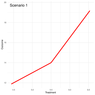
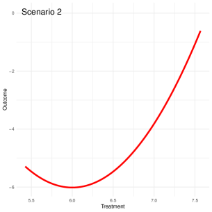
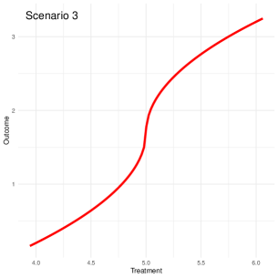
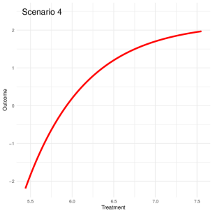
Figure 2: The four scenarios of the simulated nonlinear CERF.

Our goal is to apply our method described in the previous section to recover the true CERFs when we do not observe $U$. In Figure 3, we show the estimation results. In particular, to increase model flexibility, we define $\alpha_{k}(X)$ in (3.3) used for constructing the weights in the mixture model as a piecewise linear function of $X$. We allow the regression parameters to be different for different quartiles of $X$. Let $q_{0}=min(x)$, $q_{4}=max(x)$, and $q_{v}$ be $v$-th observed quartile cutpoints of $X$, $v=1,\dots,3$. We assume

$$\alpha_{k}(x)=\eta_{0,k}+\eta_{v,k}x\;\mbox{ for }x\in[q_{v-1},q_{v}),$$ (4.1)

where $\eta_{0,k}$ and $\eta_{v,k}$, for $v=1,\dots,3$, are distributed as $\mathcal{N}(\mu_{\eta},1)$.

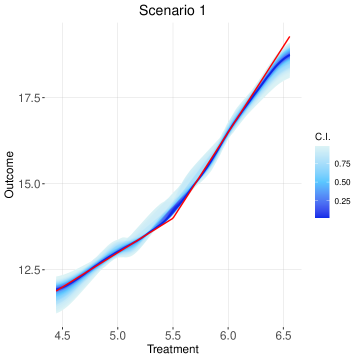
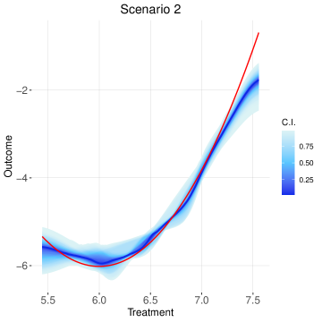
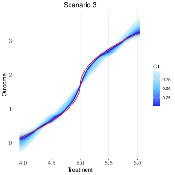
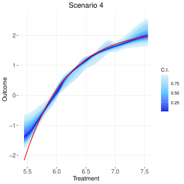
Figure 3: Comparison of the median of the estimated CERFs (the blue line) with credible intervals(CI). Red lines represent the true CERFs. Different shades of blue lines represent the width of posterior intervals ranging from the 25th to the 95th percentile.

For each scenario in Figure 2, The red line is the true CERF. the darker blue line is the median across the 300 samples of the posterior estimates of the CERF. A nice feature of our method is its ability to quantify the uncertainty in estimating the CERF. More specifically, using different shades of blue lines we present the width of posterior intervals ranging from the 25th to the 95th percentile. Figure 3 shows that the $95\%$ CIs cover the true CERFs (red curves across most of the treatment distribution’s support in these four scenarios. However, it’s worth noting that sometimes the tails are not contained in the $95\%$ CIs. Specifically, the $95\%$ CI fails to encompass the true CERF in the right tail of Scenario 2 and the left tail of Scenario 4. This discrepancy could be attributed to the scarcity of data points in those tails due to our use of Gaussian distributions for simulating $X$. In addition, we conducted a sensitivity analysis concerning the choice of the function $\alpha_{\alpha,k}(X)$ in (4.1). In the Appendix, we report our findings across the four scenarios by employing six quantiles instead of the previously used quartiles of $X$ in (4.1). The results show no notable difference when using six instead of four quantiles. Despite the slight deviation in the tails, the simulation studies demonstrate that the proposed method is very flexible in different settings when the nonlinear CERFs are of various shapes.

5 Illustration with Real Data

In this section, we illustrate how to use our method to estimate the CERF of long-term exposure to ambient $PM_{2.5}$, on cardiovascular hospitalization rates among the elderly in the continental U.S. We use the dataset gathered from Papadogeorgou and Dominici (2020) for this analysis.

The unit of our analysis is at the zip code level labeled as $i$. The outcome $Y_{i}$ is defined as the logarithm of the hospitalization rate for cardiovascular diseases (codes ICD-9 390 to 459) among Medicare beneficiaries residing in zip code $i$ during 2013. The exposure $X_{i}$ is defined as the average daily levels of ambient $PM_{2.5}$ concentrations for 2011 and 2012 recorded by EPA (U.S. Environmental Protection Agency) monitors within a 6-mile radius of zip code $i$’s centroid. The dataset does not cover all the zip codes in the continental U.S. but those within this radius of an EPA monitoring site with more than 67% of scheduled measurements. As a result, the analysis includes $N=5362$ zip codes. In addition, an extensive collection of covariates was assembled at the zip code level, including socio-economic, demographic, and cardiovascular disease risk factor information. See Table A.1. in Papadogeorgou and Dominici (2020) for detailed information on these covariates.

For illustration purposes, we consider one measured covariate, the logarithm of median household income for the zip code $i$, as an unmeasured confounder ($U$), and the benchmark CERF is the estimated CERF adjusting for $U$. To examine the performance of our approach, we mask the variable $U$ and compare whether using our BNP method with a pair of NCE and NCO variables can recover the benchmark CERF. We acknowledge the benchmark CERF is not the true CERF, which is unknown for real data applications, and we can further improve the benchmark CERF by adjusting for measured confounders that we do not consider in this example. Hence, it is important for readers to view our results not as scientific evidence for quantifying the causal effect of long-term exposure to ambient $PM_{2.5}$ on cardiovascular hospitalization rates among the elderly in the continental U.S. but as an illustration of novel statistical methods for addressing unmeasured confounding bias.

We select household income as a potential unmeasured confounder for the following reasons. Depicted by the causal diagram in Figure 4, the average household income at the zip code level $(U)$ is likely to be associated with an elevated air pollution level of $PM_{2.5}$ $(X)$ because individuals with a low income are more likely to live in low-cost areas, which could be associated with an elevated $PM_{2.5}$ level, for instance, the areas near highways. Compared to a zip code with a higher average household income, people living in a zip code with a lower average household income may also have less access to affordable health care. As a result, a low household income zip code $(U)$ may be associated with the hospitalization rate due to cardiovascular diseases $(Y)$ in this zip code.

Figure 4: The causal diagram of the unmeasured confounder $U$, the negative control exposure $Z$, and the negative control outcome $W$.

The crucial step is to select the NC variables to capture the information of the unmeasured confounders stated in assumptions A6-A7 and satisfy the conditional independence assumptions A3-A5. In the following, we demonstrate our NC variables satisfy these assumptions. We consider the percentage of the occupied population, a proxy for what proportion of the zip code residents have jobs, as our NCE variable $Z$. We consider the percentage of owner-occupied housing units in each zip code as our NCO variable $W$ . Conditional on household income $(U)$, we make the strong assumption that, for each zip code, the ambient $PM_{2.5}$ level $(X)$ is independent of the percentage of owner-occupied housing units $(W)$, the percentage of employment $(Z)$ is independent of the hospitalization rate for cardiovascular diseases among the elderly $(Y)$, and the percentage of employment $(Z)$ and the percentage of owner-occupied housing units $(W)$ are also independent (See Figure 4).

We recognize that these assumptions might not hold and are not testable in practice. For this illustrative example, however, we can check whether these assumptions hold for our data since $U$ is known. We use conditional independence tests in R package dagitty (Textor et al., 2016) developed for continuous data to check our assumptions. Because we do not assume a linear relationship between $X$ and $Y$, to test whether the data contradict the three conditional independence assumptions in A3-A5, we use a nonparametric conditional independence test for variables in this R package. Results in Table 1 show that the 95% confidence intervals of the tests for assumptions A3 and A5 cover $0$, meaning we fail to reject the null hypothesis of conditional independence. Therefore, assumptions A3 and A5 hold. The 95% confidence intervals for A4 is (-0.0619, -0.0119), meaning we barely reject the null hypothesis for A4. Given the large sample size of $N=5362$ in this example and the closeness of the confidence intervals to zero, we consider that this dataset does not violate assumption A4 much.

We then use the linear regression-based test in the same R package to check assumptions A6 and A7, which require $W$ and $U$ to be linearly correlated and $U$ and $Z$ to be linearly correlated after conditioning on $X$. Results in Table 1 show that we reject the null hypotheses that $W$ and $U$ are independent and $U$ and $Z$ are conditionally independent. Therefore, assumptions A6 and A7 also hold. Histograms are used to assess the normality assumptions of $Y,W,U$ in models (3.5) - (3.7) (results not shown). After applying log transformations to the hospitalization rate for cardiovascular diseases ($Y$) and the median household income ($U$), we verify the normality assumptions hold.

Table 1: Hypothesis Testing of Assumptions A3-A7

Assumptions	$H_{0}$	Estimate	95% CI	Conclusions
A3*	$Z\perp Y|X,U$	0.0049	[-0.0288, 0.0374]	A3 holds
A4	$X\perp W|U$	-0.0368	[-0.0619, -0.0119]	A4 almost holds
A5	$W\perp Z|U$	-0.02172	[-0.0644, 0.0238]	A5 holds
A6: $\beta_{WU}\neq 0$	$W\perp U$	0.3727	[0.3284, 0.4173]	A6 holds
A7: $\beta_{UZ}\neq 0$	$U\perp Z|X$	0.5792	[0.5571, 0.6009]	A7 holds
A3*: Here we test marginal conditional independence, slightly different from A3 in section 3.2
$X$: $PM_{2.5}$; $Y$: the logarithm of the hospitalization rate for cardiovascular diseases
$U$: the logarithm of the median household income
$Z$: the percentage of the occupied population; $W$: the percentage of owner-occupied housing units
All the hypothesis tests are two-sides conducted at the significance level of 0.05

We fit three models to the data for comparison. The first model, denoted as “YX” in Figure 5, does not consider the unmeasured confounder $U$ and assumes

$$Y|X\sim\sum_{k\geq 1}w_{k}(X)\mathcal{N}(\beta_{0,k}+\beta_{X,k}X).$$

In the second model denoted as “YXU” in Figure 5, we unmask $U$ and fit the BNP model, adjusting for $U$ by treating it as a covariate. $U$ is allowed to have a nonlinear relationship with $Y$:

$$Y|X,U\sim\sum_{k\geq 1}w_{k}(X)\mathcal{N}(\beta_{0,k}+\beta_{X,k}X+\beta_{u,k}U).$$

The third model, denoted as “BNP-NC”, accounts for the $U$ without using $U$. We apply our BNP method described in section 3, incorporating NCs to adjust for $U$.

Figure 5 shows the estimated response functions using these three models and the 95% CI of the estimate curves. We consider the response function estimated from the “YXU” model our benchmark and use it to evaluate the performance of a proposed method. When the covariate $U$ is masked, the estimated response curve from the “BNP-NC” model (the blue line and interval) is close to the benchmark “YXU” result (the green line and interval), demonstrating our method’s effectiveness. Figure 5 also shows there is a discrepancy between the response function estimated from the “YX” model (the orange line and interval) and the benchmark “YXU” result (the green line and interval), highlighting the danger of not accounting for unmeasured confounding from $U$.

It is worth noting a scarcity of data when the $PM_{2.5}$ exposure level is below 7.5 $\mu g/m^{3}$ or greater than 12.5 $\mu g/m^{3}$ (Figure 5). Given our method’s slightly weaker performance when the data size is small in the tail sections of the exposure as demonstrated in simulation studies, we suggest focusing on the central portion of the estimated CERF when evaluating a method with this example data. Examining the central section of the data distribution in Figure 5, we observe that the blue line indicating our proposed method is still closer to the green line, representing the benchmark, than the orange line indicating the other method, demonstrating the superior performance of our method.

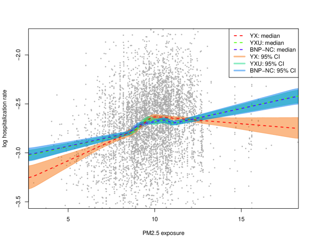
Figure 5: The estimated response functions (dotted lines) and their 95% credible intervals (colored areas) based on three models.“YXU”, colored in green, indicates the result from the BNP method adjusting for a confounder $U$ when $U$ is unmasked. “YX”, colored in orange, indicates the result from the BNP method without considering the confounder $U$.“BNP-NC”, colored in green, indicates the result from the BNP method using NCs to adjust for unmeasured confounders when $U$ is masked.

6 Discussion

We develop a method to estimate the CERF denoted by $E[Y(x)]$ in the presence of an unmeasured confounder $U$ for the continuous exposure $X$ and continuous outcome $Y$. We address three challenges in this causal inference problem summarized below:

1. $U$ is a latent variable that standard causal inference techniques for confounding adjustment using either matching or inverse probability weighting do not apply. We solve this problem by using a pair of auxiliary variables, $Z$ and $W$, which are often easy to obtain and sometimes already available among the collected covariates, as shown in our illustration with real data.

2. The response function $Y$ to a continuous variable $X$ is often non-linear and varies in different applications. Using one parametric model to capture all possible shapes of a response function is difficult. Our approach is to adopt a Bayesian nonparametric mixture model, which can handle an arbitrary response curve shape.

3. There is currently no method to incorporate NCs (or proxy variables) into a Bayesian nonparametric method to account for unmeasured confounding. We fill this methodology gap by modeling $Y$’s response to $X$ of an arbitrary shape 1) using a mixture of linear models and 2) leveraging a proximal causal inference result for linear models that provides a closed-form solution when estimating the causal effect in the presence of $U$.

Our simulation studies have shown that our method can recover the true CERF of various shapes with finite samples in the presence of unmeasured confounding, providing an alternative solution to machine learning approaches that may require a large sample size to perform well. We illustrate how to use our method by applying it to studying the relationship between long-term exposure to ambient $PM_{2.5}$ on cardiovascular hospitalizations among the elderly in the continental U.S., showing the difference between using and without using our method and highlighting the danger of not accounting for unmeasured confounders.

There are several limitations in our methodology for future improvement. First, although we allow the confounding effect of $U$ on the outcome $Y$ to be nonlinear in our model, we assume a linear relationship between $U$ and the NCO variable $W$, and between $U$ and the NCE variable $Z$. Such restrictions can be relaxed by using BNP models to define these relationships as how we model the outcome $Y$. Second, we assume the conditional independence condition in A3 holds for each mixture component. Yet, our method performs well in the real-data example even when A3 only marginally holds for variables $Y$, $X$, and $Z$. It is of theoretical interest to explore whether assumption A3 can be relaxed to a marginal assumption when data follow Gaussian distributions. Third, simulation studies show that the performance of our method deteriorates toward the tails of the CERF, possibly due to 1) fewer data at the small and large values of the exposure $X$ because we simulate $X$ using Gaussian distributions; 2) the fitted BNP models with NCs are too smooth at the tails. To increase model flexibility, we construct the weights of the mixture model such that they depend on $X$ and further allow the relationship of this dependence to vary in different quantiles of $X$ (4.1). However, our method could be easily extended to accommodate weight dependence on NCs or other covariates, which may further increase model flexibility and, potentially the performance in the tails of the response functions.

In conclusion, our proposed method, which combines Bayesian nonparametric methods with the proximal causal inference framework, offers a powerful tool for estimating the CERF in the presence of unmeasured confounding. Our simulation studies demonstrate our method’s effectiveness with finite sample sizes, and our real-data application example showcases its practical utility in addressing a common problem in observational studies.

7 Acknowledgement

This work was supported by the National Institute Environmental Health Sciences grant (T32 ES 7069), Sloan Foundation grant (G-2020-13946), and the National Institute Health grants (R01ES028033, 1R01ES030616, 1R01ES029950, R01MD012769, 1RF1AG074372-01A1, 1RF1AG080948, 1RF1AG071024).

SUPPLEMENTARY MATERIAL

Appendix A Priors, Posteriors, and Gibbs Sampling

In the following, we describe our Bayesian inference framework. First, we complete the definition of the model in Section 3.2 with the clarification of the prior distributions for the parameters.

Let $\mathcal{N}_{c}(a,b\cdot\mathbf{1}_{c})$ denote a $c$-variate Gaussian distribution with the mean vector $a$ and the covariance matrix $b\cdot\mathbf{1}_{c}$, i.e., a $c\times c$ diagonal matrix. With this notation, we assume independence among components of the vector and all components have the same variance $b$.

We assume the priors for ${\boldsymbol{\eta}}_{k}$ in the weight model follow:

$${\boldsymbol{\eta}}_{k}\stackrel{{\scriptstyle iid}}{{\sim}}\mathcal{N}_{p}(\mu_{\eta,k},\sigma_{\eta}^{2}\cdot\mathbf{1}_{p}),\mbox{ for }k=1,2,\dots,K.$$ (A.1)

where ${\boldsymbol{\eta}}_{k}$ is the $p$-dimensional parameter vector in the probit regression model for the weights of the mixture model.

We assume the priors for the parameters ${\boldsymbol{\theta}}_{Y,k}$ and $\delta_{y,k}$ in model (3.11) for $Y|X,Z$ follow

$${\boldsymbol{\theta}}_{Y,k} \stackrel{{\scriptstyle iid}}{{\sim}}\mathcal{N}_{3}(\mu_{\theta},\sigma_{\theta}^{2}\cdot\mathbf{1}_{3}),\mbox{ for }k=1,2,\dots,K;$$

$$\delta_{y,k} \stackrel{{\scriptstyle iid}}{{\sim}}\mbox{InvGamma}(\gamma_{1},\gamma_{2}),\mbox{ for }k=1,2,\dots,K;$$ (A.2)

where ${\boldsymbol{\theta}}_{Y,k}=(\theta_{0,k},\theta_{X,k},\theta_{Z,k})$ are the component-specific regression parameters in the kernels of the mixture model, $\delta_{y,k}$ is the component-specific variance parameter for the kernels. We assume the prior for $\delta_{y,k}$ follows an inverse-gamma distribution with the shape parameter $\gamma_{1}$ and the scale parameter $\gamma_{2}$, with mean equal to $\frac{\gamma_{2}}{\gamma_{1}-1}$ and variance $\frac{\gamma_{2}^{2}}{(\gamma_{1}-1)^{2}(\gamma_{1}-2)}$.

We assume the priors for ${\boldsymbol{\theta}}_{W}$ and $\delta_{w}$ in the model (3.12) for $W|X,Z$ distribution follow:

$${\boldsymbol{\theta}}_{W} \sim\mathcal{N}_{3}(\mu_{\theta},\sigma_{\theta}^{2}\cdot\mathbf{1}_{3});$$

$$\delta_{w} \sim\mbox{InvGamma}(\gamma_{3},\gamma_{4}),$$ (A.3)

where ${\boldsymbol{\theta}}_{W}=(\theta_{W0},\theta_{WX},\theta_{WZ})$ are the regression parameters in the model (3.6) for $W|X,Z$ .

The distributions in (A.1)-(A.3) are conjugate priors that allow us to obtain the posterior distributions for the parameters involved conveniently. Consequently, we can estimate them with an efficient Gibbs sampling algorithm.

The Gibbs sampling algorithm was outlined in Algorithm 1 1. In each iteration $r=1,\dots,R$, it first draws from the posterior distributions of the parameters and then computes $E[Y(x)]$ following the result in (3.15). Below are the detailed steps:

• Draw from the posterior distributions for the parameters in the model of $Y|X,Z$ and the latent variables $S$ involved:

  • Component allocation: the posterior distribution of the latent variables $S_{i}$ follows a multinomial distribution:

    $$Pr(S_{i}=k)\propto\omega_{k}(x_{i})\mathcal{N}(y_{i};\theta_{0,k}+\theta_{X,k}x_{i}+\theta_{Z,k}z_{i},\delta_{y,k}^{2}),\mbox{ for }k=1,\dots,K;$$

    with $\omega_{k}(x_{i})=\Phi(\alpha_{k}(x_{i}))\prod_{r<k}(1-\Phi(\alpha_{r}(x_{i}))),$ for $k=1,\dots,K$ and $i=1,\dots,n$, where $\alpha_{k}(x_{i})=\eta_{0,k}+\eta_{v,k}x_{i}\;\mbox{ for }x\in[q_{v-1},q_{v})$ and $\Phi(\alpha_{k}(x_{i}))=1$ for k =K.

  • Component-specific parameters: Conditional on the latent variables $\{S_{i}\}_{i=1}^{n}$, we can update the values of the parameters from their posterior distributions, for $k=1,\dots,K$:

    $${\boldsymbol{\theta}}_{Y,k} \sim\mathcal{N}\left(V_{k}\cdot\left(\frac{\mu_{\theta}}{\sigma_{\theta}^{2}}+\frac{\sum_{i\in\{S_{i}=k\}}y_{i}\cdot(\theta_{0,k}+\theta_{X,k}x_{i}+\theta_{Z,k}z_{i})}{\delta^{2}_{y,k}}\right),V_{k}\right)$$

    $$\mbox{ where }V_{k} =\frac{1}{\sigma_{\theta}^{2}}\cdot\mathbf{1}_{3}+\frac{[1,x_{i\in\{S_{i}=k\}},z_{i\in\{S_{i}=k\}}]^{T}[1,x_{i\in\{S_{i}=k\}},z_{i\in\{S_{i}=k\}}]}{\delta_{y,k}^{2}},$$

    $$\delta_{y,k}^{2} \sim\mbox{InvGamma}\left(\gamma_{1}+\frac{n_{k}}{2},\gamma_{2}+\frac{\sum_{i\in\{S_{i}=k\}}[y_{i}-(\theta_{0,k}+\theta_{X,k}x_{i}+\theta_{Z,k}z_{i})]^{2}}{2}\right),$$

    and $n_{k}$ is the number of units allocated to the mixture component $k$.

  • Augmentation scheme: In order to sample from $\{\alpha_{k}(x)\}_{k=1}^{K}$ we use the data augmentation scheme, developed by Albert and Chib (2001) and borrowed by Rodriguez and Dunson (2011). We can impute the augmented variables $\{Q_{k}(x_{i})\}_{k=1}^{\max(S_{i},K-1)}$, for each $i$, by sampling from its full conditional distribution:

    $$Q_{k}(x_{i})|S_{i},\alpha_{k}(x_{i})\sim\begin{cases}\mathcal{N}(\alpha_{k}(x_{i}),1)\mathbf{I}_{\mathrm{R}^{+}}\mbox{ if }S_{i}=k,\\ \mathcal{N}(\alpha_{k}(x_{i}),1)\mathbf{I}_{\mathrm{R}^{-}}\mbox{ if }S_{i}<k;\end{cases}$$

    where $\alpha_{k}(x_{i})$ is updated using the the new values of $\omega_{k}(x_{i})$ by

    $$\alpha_{k}(x_{i})=\phi\left(\frac{\omega_{k}(x_{i})}{\prod_{r<k}(1-\Phi(x_{i}^{T}{\boldsymbol{\eta}}_{r})}\right)=\phi\left(\frac{\omega_{k}(x_{i})}{1-\sum_{r<k}\omega_{r}(x_{i})}\right);$$

    $\phi(\cdot)$ is the density function of the Gaussian distribution.

  • Weights: The posterior distribution for ${\boldsymbol{\eta}}_{k}$, for $k=1,\dots,\max(S_{i},K-1)$, is:

    $${\boldsymbol{\eta}}_{k}\sim\mathcal{N}\left(\left(\frac{1}{\sigma^{2}_{\eta}}\mathbf{1}_{p}+\tilde{x}_{k}^{T}\tilde{x}_{k}\right)^{-1}\cdot\left(\frac{\mu_{\eta}}{\sigma_{\eta}^{2}}+\tilde{x}_{k}^{T}\tilde{Q}_{k}\right),\left(\frac{1}{\sigma^{2}_{\eta}}\mathbf{1}_{p}+\tilde{x}_{k}^{T}\tilde{x}_{k}\right)^{-1}\right)$$

    where $\tilde{x}_{k}$ is a matrix composed by the rows $[1,x_{i}]$, $i\in\{S_{i}\leq k\}$ and $\tilde{Q}_{k}$ is a vector composed by the $Q_{k}(x_{i})$, $i\in\{S_{i}\leq k\}$.

• Draw from the posterior distribution of the parameters in the $W|X,Z$ model:

  $$\boldsymbol{\theta}_{W} \sim\mathcal{N}_{3}\biggl{(}V^{-1}\biggl{(}\frac{1}{\sigma^{2}_{\theta}}\mu_{\theta}+\frac{1}{\delta^{2}_{w}}[1,x,z]^{T}w\biggl{)},V^{-1}\biggl{)}$$

  $$V =\frac{1}{\sigma^{2}_{\theta}}\mathbf{1}_{3}+\frac{1}{\gamma^{2}_{w}}[1,x,z]^{T}[1,x,z];$$

  $$\delta^{2}_{w} \sim\mbox{InvGamma}\left(\gamma_{3}+\frac{n}{2},\gamma_{3}+\frac{\sum_{i=1}^{n}(w_{i}-(\theta_{W0}+\theta_{WX}x_{i}+\theta_{WZ}z_{i}))^{2}}{2}\right).$$

  $n$ is the total sample size and $x$, $z$, $w$ are the observed values of $n$-dimension for variables $X$, $Z$, and $W$.

• According to (3.13)-(3.14), identify the parameters for the causal effect regression for $k=1,\dots,K$, namely the slope $\beta_{x,k}$ and the intercept $\iota_{k}$ as follows, respectively:

  $$\beta_{x,k} =\theta_{X,k}-\theta_{Z,k}\frac{\theta_{WX}}{\theta_{WZ}},$$

  $$\iota_{k} =\theta_{0,k}+\theta_{Z,k}\cdot\sum_{i=1}^{n}\frac{z_{i}}{n}+\theta_{Z,k}\frac{\theta_{WX}}{\theta_{WZ}}\cdot\sum_{i=1}^{n}\frac{x_{i}}{n}.$$

Appendix B Sensitivity Analysis

With the goal of understanding the sensitivity of the model to the choice of the function of $\mu_{\alpha}(X)$ (B.1)—i.e. the mean of the variable $\alpha$ involved in the weights of the mixture model—we have also estimated the model defining, for the four settings reported in Section 4, we have also estimated the model defining using the following definition of $\mu_{\alpha}(X)$.

Let $q_{0}=min(x)$, $q_{6}=max(x)$, and $q_{v}$ be $v$-th observed 6-quantiles cutpoints of $X$ where $v=1,\dots,5$. We assume

$$\alpha_{k}(x)=\eta_{0,k}+\eta_{v,k}x\;\mbox{ for }x\in[q_{v-1},q_{v})$$ (B.1)

where $\eta_{0,k}$ and $\eta_{v,k}$, for $v=1,\dots,3$, are distributed as $\mathcal{N}(\mu_{\eta},1)$.

Figure B.1 reports the comparison between the true CERF and the estimated CERF: median posterior and credible intervals.

The posterior CERFs for the four scenarios in Figure B.1 have similar behavior to the posterior CERFs in Figure 3 in Section 4. However, the estimation of CERFs is still poor at the tails of the $X$, in particular for the right tail in Scenario 1 and Scenario 2 and the left tail in Scenario 4, where the $95\%$ credible interval does not include the true CERF.

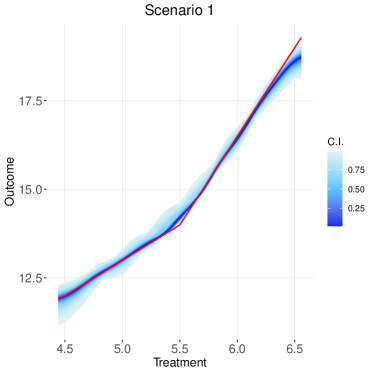
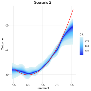
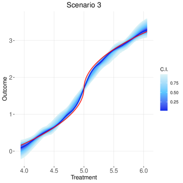
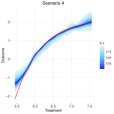
Figure B.1: Comparison of the estimated CERF (the continuous blue line) with credible intervals—C.I.—(colored area: from dark blue for 0$\%$ to light blue $95\%$) and the true CERF (the continuous red line).

References

- Albert and Chib (2001) Albert, J. H. and Chib, S. (2001). “Sequential ordinal modeling with applications to survival data.” Biometrics, 57(3): 829–836.
- Chung and Dunson (2009) Chung, Y. and Dunson, D. B. (2009). “Nonparametric Bayes conditional distribution modeling with variable selection.” Journal of the American Statistical Association, 104(488): 1646–1660.
- Cui et al. (2023) Cui, Y., Pu, H., Shi, X., Miao, W., and Tchetgen Tchetgen, E. (2023). “Semiparametric proximal causal inference.” Journal of the American Statistical Association, (just-accepted): 1–22.
- Ghassami et al. (2022) Ghassami, A., Ying, A., Shpitser, I., and Tchetgen, E. T. (2022). “Minimax Kernel Machine Learning for a Class of Doubly Robust Functionals with Application to Proximal Causal Inference.”
- Hu et al. (2023) Hu, J. K., Tchetgen Tchetgen, E. J., and Dominici, F. (2023). “Using negative controls to adjust for unmeasured confounding bias in time series studies.” Nature Reviews Methods Primers, 3(1): 66.
- Kallus et al. (2022) Kallus, N., Mao, X., and Uehara, M. (2022). “Causal Inference Under Unmeasured Confounding With Negative Controls: A Minimax Learning Approach.”
- Kompa et al. (2022) Kompa, B., Bellamy, D. R., Kolokotrones, T., Robins, J. M., and Beam, A. L. (2022). “Deep Learning Methods for Proximal Inference via Maximum Moment Restriction.”
- Lipsitch et al. (2010) Lipsitch, M., Tchetgen, E. T., and Cohen, T. (2010). “Negative controls: a tool for detecting confounding and bias in observational studies.” Epidemiology (Cambridge, Mass.), 21(3): 383.
- Mastouri et al. (2023) Mastouri, A., Zhu, Y., Gultchin, L., Korba, A., Silva, R., Kusner, M. J., Gretton, A., and Muandet, K. (2023). “Proximal Causal Learning with Kernels: Two-Stage Estimation and Moment Restriction.”
- Miao et al. (2018) Miao, W., Geng, Z., and Tchetgen Tchetgen, E. J. (2018). “Identifying causal effects with proxy variables of an unmeasured confounder.” Biometrika, 105(4): 987–993.
- Papadogeorgou and Dominici (2020) Papadogeorgou, G. and Dominici, F. (2020). “A causal exposure response function with local adjustment for confounding: Estimating health effects of exposure to low levels of ambient fine particulate matter.” The annals of applied statistics, 14(2): 850.
- Rodriguez and Dunson (2011) Rodriguez, A. and Dunson, D. B. (2011). “Nonparametric Bayesian models through probit stick-breaking processes.” Bayesian analysis (Online), 6(1).
- Shi et al. (2020a) Shi, X., Miao, W., Nelson, J. C., and Tchetgen Tchetgen, E. J. (2020a). “Multiply robust causal inference with double-negative control adjustment for categorical unmeasured confounding.” Journal of the Royal Statistical Society Series B: Statistical Methodology, 82(2): 521–540.
- Shi et al. (2020b) Shi, X., Miao, W., and Tchetgen, E. T. (2020b). “A selective review of negative control methods in epidemiology.” Current epidemiology reports, 7: 190–202.
- Singh (2023) Singh, R. (2023). “Kernel Methods for Unobserved Confounding: Negative Controls, Proxies, and Instruments.”
- Tchetgen et al. (2020) Tchetgen, E. J. T., Ying, A., Cui, Y., Shi, X., and Miao, W. (2020). “An Introduction to Proximal Causal Learning.”
- Textor et al. (2016) Textor, J., van der Zander, B., Gilthorpe, M. S., Liśkiewicz, M., and Ellison, G. T. (2016). “Robust causal inference using directed acyclic graphs: the R package ’dagitty’.” International Journal of Epidemiology, 45(6): 1887–1894.
- Xu et al. (2021) Xu, L., Kanagawa, H., and Gretton, A. (2021). “Deep proxy causal learning and its application to confounded bandit policy evaluation.” Advances in Neural Information Processing Systems, 34: 26264–26275.