Superclustering by finding statistically significant separable groups of optimal gaussian clusters

Abstract

The paper presents the algorithm for clustering a data set by grouping the optimal, from the point of view of the Bayesian information criterion, number of Gaussian clusters into the optimal, from the point of view of their statistical separability, superclusters.

The algorithm consists of three stages: representation of the data set as a mixture of Gaussian distributions - clusters, which number is determined based on the minimum of the Bayesian information criterion; using the Mahalanobis distance to estimate the distances between the clusters and cluster sizes; combining the resulting clusters into superclusters using the density-based spatial clustering of applications with noise method by finding its maximum distance hyperparameter providing maximum value of introduced matrix quality criterion at maximum number of superclusters. The matrix quality criterion corresponds to the proportion of statistically significant separated superclusters among all found superclusters.

The algorithm has one hyperparameter - statistical significance level, and automatically detects optimal number and shape of superclusters based of statistical hypothesis testing approach. The algorithm demonstrates a good results on test data sets in noise and noiseless situations. An essential advantage of the algorithm is its ability to predict correct supercluster for new data based on already trained clusterer and perform soft clustering. The disadvantages of the algorithm are: its low speed and stochastic nature of the final clustering. It requires a sufficiently large data set for clustering, which is typical for many statistical methods.

1 Introduction

Data clustering algorithms [13] are usually divided into two big categories: hierarchical and partitional. Hierarchical methods are based either on joining close clusters (agglomerative methods) or separating big clusters (divisive methods). Partitinal methods can be divided on distance based, model based and density based. Model-based ones describe the data by a combination of statistical distribution functions, for example EM algorithm for the mixture of normal distributions [11]. The basis of distance methods is the pairwise distance between points, for example spectral clustering [7]. The popular density method is Density-based spatial clustering of applications with noise (DBSCAN), suggested in [3], and discussed in [14]. Comparison of different methods can be found in [10, 12].

Most of the methods have one or more hyperparameters [12] - for DBSCAN this is the maximum distance between a pair of objects, for K-means[1], for Spectral[7] and Gaussian Mixture, this is the number of classes. One of the main tasks for a researcher is to choose a clustering method and find the hyperparameters values that provide the best solution of his clustering problem.

The choice of a clusterer is related to the data model - the clusterer that is optimal for the researcher should correspond to the data. On the one hand, it should have the necessary freedom to correctly describe the data set for any expert separation of the data set into a clusters - in terms of the Kleinberg theorem [4] - to provide richness. On the other hand it should correctly label the original unlabeled data set so that the number and shape of clusters coincide with what an expert expect from the data set.

Let us explain the main idea of the algorithm, suggested in the paper. A data set consisting of two expert-labeled classes can be separated into an arbitrary number of clusters, and by many ways.

Let us consider the Rand index [9] at data set $S$ in classification (not clusterization) problem:

$$RI=\frac{TP+TN}{C_{2}^{N}}$$ (1)

where TP (True Positive) is the number of pairs of elements that are in the same clusters in set $S_{l}$ (data set $S$, labeled by an expert) and in the same cluster in set $S_{c}$ (data set $S$, clustered by an algorithm); TN (True Negative) is the number of pairs of elements that are in different clusters in set $S_{l}$ and in different clusters in set $S_{c}$; $C_{2}^{N}$ - total number of pairs in data set $S$.

In this case, pairwise true positive (PWTP) metric can be defined as:

$$PWTP=\frac{TP}{C_{2}^{N}}$$ (2)

and pairwise true negative (PWTN) metric can be defined as:

$$PWTN=\frac{TN}{C_{2}^{N}}$$ (3)

Rand Index is sum of PWTP and PWTN. Obviously, the easiest way to achieve the maximum of PWTN metric, is to put each point into its own separate cluster, but PWTP metric in this variant will become zero. The easiest way to achieve the maximum of PWTP metric, is to put all the points into the same single cluster, but PWTN metric in this variant will become zero.

Let us refer the optimal PWTN algorithm as the algorithm providing maximum PWTN, and refer the optimal PWTP algorithm as the algorithm providing maximum PWTP. We suggest that by corresponding grouping clusters produced by optimal PWTN algorithm we can obtain optimal PWTP algorithm without loosing its PWTN optimality. Adequate classification can be defined as a classification that is both optimally PWTP and optimally PWTN with respect to the teacher’s labeling. It is obvious that this corresponds to the absolute maximum of RI because in this case the errors of the first and second kind (FN, FP) are equal to zero. The absolute maximum of both PWTP and PWTN metrics is reached simultaneously when the number of classes in the labeled data set $S_{l}$ and classified data set $S_{c}$ are the same, and their shapes are also the same. Therefore, the adequate classification problem in the presence of a labeled data set $S_{l}$ can be considered as the problem of achieving RI its absolute maximum value of 1. A good approximation to adequate classification can be found by supervised learning, when $S_{l}$ is given.

However, in most cases, it seems to be impossible to achieve adequate clustering by unsupervised learning. We do not know the set $S_{l}$, and therefore RI will be most likely less than 1 due to the imperfection of our knowledge about $S_{l}$. Therefore, each clustering model has its own limitations - our initial assumptions about the unknown set $S_{l}$: K-Means searches for centroids, DBSCAN for distance separated points, Gaussian Mixture for points which distributions are close to normal ones.

Approximation by Gaussian distributions is widely used in clustering because potentially it can provide a high PWTN metric - an infinite sum of Gaussian distributions can fit (and separate) any arbitrary discrete set of points.

This paper demonstrates an algorithm that uses grouping of gaussian clusters into superclusters to create a clustering close to adequate one, based on our own assumptions about the set $S_{l}$, that will be explained later.

2 Algorithm

2.1 The idea

We will solve the problem sequentially: at the first stage, we will approximate our data most accurately by the optimal number of clusters from the point of view of likelihood (we will construct a clustering with a potentially high PWTN metric). At the second stage we will group these clusters into the optimal number of superclusters (we will increase PWTP metric) from the point of view of the distance between these superclusters. Optimality in terms of likelihood at the first stage should allow us to best separate the data clusters from a statistical point of view, and at the second stage we group too close clusters. The problem conceptually is close to the well-known hierarchical method - agglomerative clustering[17], but uses only two stages instead of using their sequence.

Important requirements for our algorithm are: robustness to a noise, interpretability of each of its stages in terms of a statistical approach, and minimizing the number of hyperparameters.

The first stage can be simply solved when we are not limited by the maximum number of clusters: we can choose the number of clusters equal to the number of objects and place each object in its own cluster. If we want to limit the number of clusters we need to use some kind of clustering as an initial stage. We choose an approximation by mixture of normal distributions - Gaussian Mixture (GM). The advantage of this method is that it is statistical one. Another advantage - it has a widely used criterion for finding the optimal number of objects - the Bayesian Information Criterion - BIC [15]. Therefore, we expect that most likely the optimal number of initial clusters will be less than the number of points (objects) in the data set. The disadvantage of this method is its stochastic nature associated with the iterative Expectation-Maximization (EM) algorithm used for search of GM parameters, and dependence of EM results on its stochastic initial state [11].

The second stage is close to agglomerative clustering. The main principle of agglomerative clustering is sequential grouping of the closest clusters. In agglomerative approach, one should group them until all the clusters are grouped into a single supercluster, or until necessary number of superclusters is reached, or until optimum of a certain criterion is reached.

Therefore two main problems arise: by what principle to combine clusters, and by what criteria to detect if the clustering becomes the optimal one. There are many methods for solving the first problem. The simplest method is sequential one - greedy joining. In this case, we find a pair of closest clusters, and group them into one [17]. Another common method is density based distribution (DBSCAN). However, DBSCAN has problems in choosing value of a hyperparameter - the maximum distance between points in a cluster ($\varepsilon$). So one need to vary (or to use some search method) to find optimal $\varepsilon$, which slows down the algorithm. We choose DBSCAN method due to it is easy to implement.

The second problem is the choice of metric - the distance between clusters. Since we use GM, one of the native metrics is the Mahalanobis distance [5], which scales the space depending on the covariance matrix of the found Gaussian distribution. The distance between two clusters can also be calculated using in terms of this metric. Our algorithm stops when the distance between all found superclusters exceeds a given threshold level. Mahalanobis distance is widely used in solving classification problems, for example in Quadratic Discriminant Anaysis [6].

The name of our algorithm (GMSDB) is formed from the three elements it based on: Gaussian Mixture (GM), statistical approach (S) and DBSCAN (DB). Let us describe the GMSDB algorithm in details.

2.2 Stage 1: Data approximation by the optimal GM

At this stage, we iterate over the number of clusters $N$ until the minimum of the BIC criterion[15] is reached, or until the number of clusters reaches a high enough value that we have specified. In this stage, we assume that the set of points $\overrightarrow{x}$ satisfies the distribution with the probability density $P_{GM}(\overrightarrow{x})$:

$$P_{GM}(\overrightarrow{x})=\sum_{n=1}^{N}A_{i}P(\overrightarrow{x}|\theta_{i})$$ (4)

$$\sum_{n=1}^{N}A_{i}=1$$ (5)

Here $P(\overrightarrow{x}|\theta_{i})$ is the normal distribution described by the set of its unknown parameters $\theta_{i}$ (mean and covariance matrix), and unknown weights $A_{i}$ of the corresponding distribution in the sum. N is the number of distributions in the mixture. The optimal distributions $P_{GM}(\overrightarrow{x})$ and $P(\overrightarrow{x}|\theta_{i})$, as well as $N=N_{BIC},A_{i},\theta_{i}$, at which the minimum of the BIC criterion is reached, will be the result of this stage.

Figure 1 shows examples of the BIC dependence on the number of clusters $N$ and the resulting splitting of the original data set into the optimal number $N_{BIC}$ of Gaussian clusters $P(\overrightarrow{x}|\theta_{i})$, as well as decision regions, defining the boundaries between these clusters. Obviously, only the first example (’blobs’, shown Figure 1A) is an adequate enough model; the other cases (Figure 1B-D) are just some clusterings with high enough PWTN.

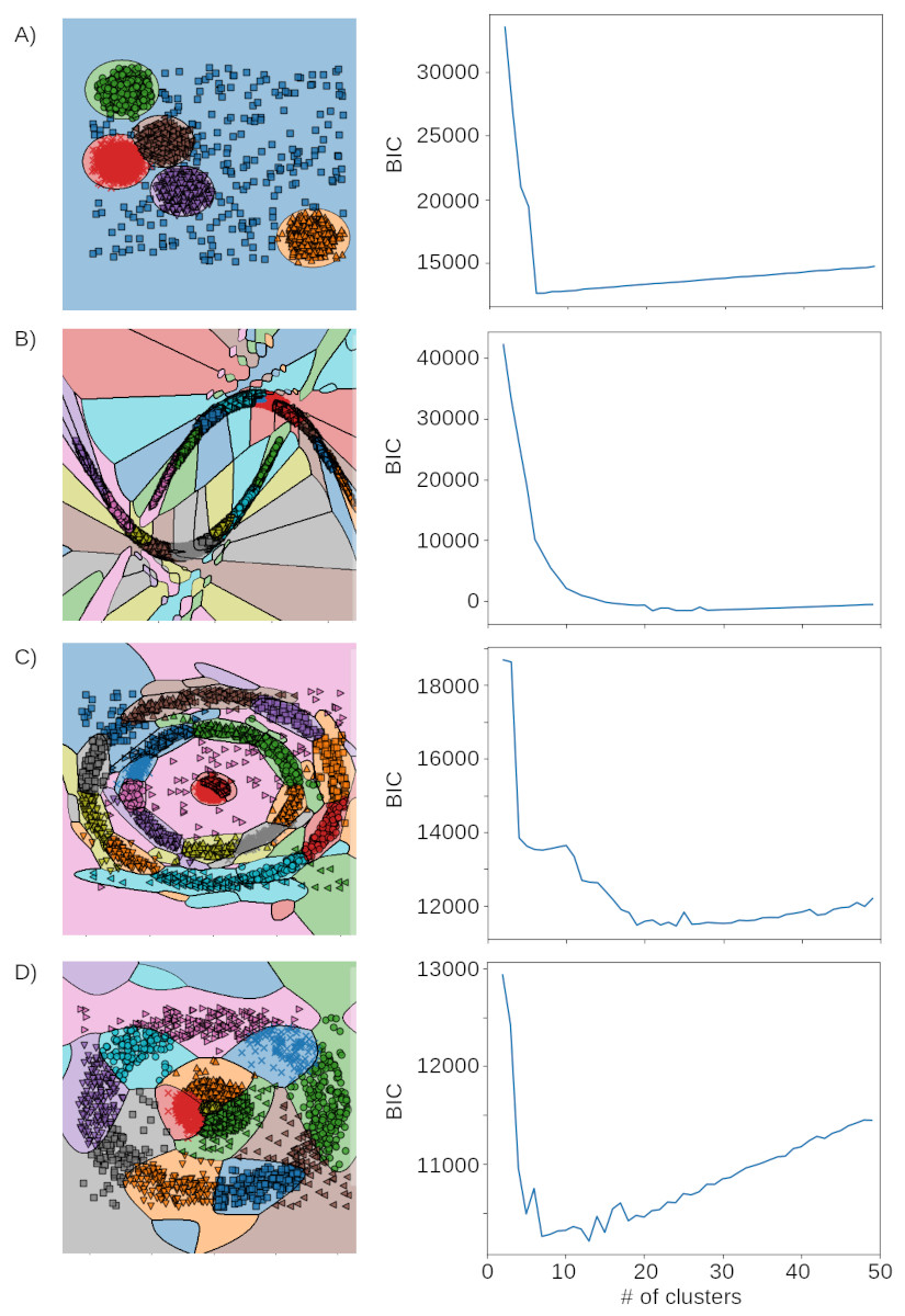
Figure 1: Clustering points into BIC-optimal mixture of Gaussian distributions. On the left is a separation by the number of clusters $N_{BIC}$ corresponding to the BIC minimum. The background corresponds to decision areas, all points of which the algorithm will refer to given cluster. Colors correspond to different clusters. On the right is the dependence of BIC on the number of clusters. A) ’medium blobs’; B) ’two horseshoes’; C) ’three nested rings with noise’; D) ’two nested rings with noise’

2.3 Stage 2: Calculation of intercluster distances

We require the algorithm to be robust to a noise and interpretable from statistical point of view. So metrics should be carried out not in Euclidean space, but in probability space. We used a mixture of Gaussian distributions so the distance between clusters and cluster sizes are calculated using Mahalanobis distances [5], native for gaussian statistical distribution:

$$p_{ij}=\sqrt{(\overrightarrow{x_{i}}-\overrightarrow{y_{j}})S_{j}^{-1}(\overrightarrow{x_{i}}-\overrightarrow{y_{j}})^{T}}$$ (6)

where $S_{j}^{-1}$ is the matrix inverse to the covariance matrix of the cluster to which point $\overrightarrow{y_{j}}$ belongs.

The distance is widely used in different clustering and classification tasks [16, 6]. Qualitatively, the Mahalanobis distance is the distance from a point $\overrightarrow{x}$ to an ellipsoid normalized to the ellipsoid width. Therefore it could be qualitatively interpreted as t-statistic value[18]. Thus, the Mahalanobis distance can be used as a statistic for testing the hypothesis that the point $\overrightarrow{x}$ belongs to a given normal distribution, to which $\overrightarrow{y}$ belongs. When it reaches a certain threshold value, we can talk about the rejection of this hypothesis with the corresponding statistical significance level.

The Mahalanobis distance is usually defined for the case when both points are from the same distribution. We will use points from different distributions (clusters). Accordingly, their covariance matrices ($S_{j}$ and $S_{i}$) in the general case will be different, and the distance calculated (6) will not be a distance, since it is not symmetrical:

$$\sqrt{(\overrightarrow{x_{i}}-\overrightarrow{y_{j}})S_{j}^{-1}(\overrightarrow{x_{i}}-\overrightarrow{y_{j}})^{T}}\neq\sqrt{(\overrightarrow{x_{i}}-\overrightarrow{y_{j}})S_{i}^{-1}(\overrightarrow{x_{i}}-\overrightarrow{y_{j}})^{T}}$$ (7)

In this case, when analyzing points from two clusters, we have 4 statistical distributions of these quasi-metrics: $p_{ii},p_{jj},p_{ji},p_{ij}$, where the indices i,j correspond to the points in i-th and j-th clusters, obtained in Stage 1 GM/BIC clusterization (4). The distributions of $p_{ii},p_{jj}$ can be used for calculating the cluster sizes, and of $p_{ij},p_{ji}$ - for calculating intercluster distances with taking into account the j-th and i-th cluster shapes, respectively.

The intercluster distance $R_{ij}$ must be symmetrical ($R_{ij}=R_{ji}$), so we should form a symmetric function from $p_{ij},p_{ji}$ distributions. As the intercluster distance we choose the maximum between 5-th percentiles:

$$\begin{array}[]{c}R_{ij}=Max(Percentile_{5\%}(p_{ij}),Percentile_{5\%}(p_{ji}))\\ R_{ii}=0\end{array}$$ (8)

The 5th percentile (5%) was chosen for statistical reasons and corresponds to the lower limit, below which, with a standard statistical confidence level of 95%, the distance between points in these clusters does not fall down. In addition, percentiles are more robust to outliers than standard deviations and means. The maximization between two values is used to symmetrize the distance $R_{ij}$. It corresponds to the transition to the coordinate system of the cluster in which the intercluster distance is higher, and the two clusters can be more confidently separated.

Figure 2A-D shows examples of clusters and their corresponding Mahalanobis distance distributions (6). It can be seen from the figure that the distance distributions $p_{ij}$ and $p_{ji}$ generally do not coincide, which explains distance symmetrization (8). The scheme for determining distances is illustrated in Figure 2E.

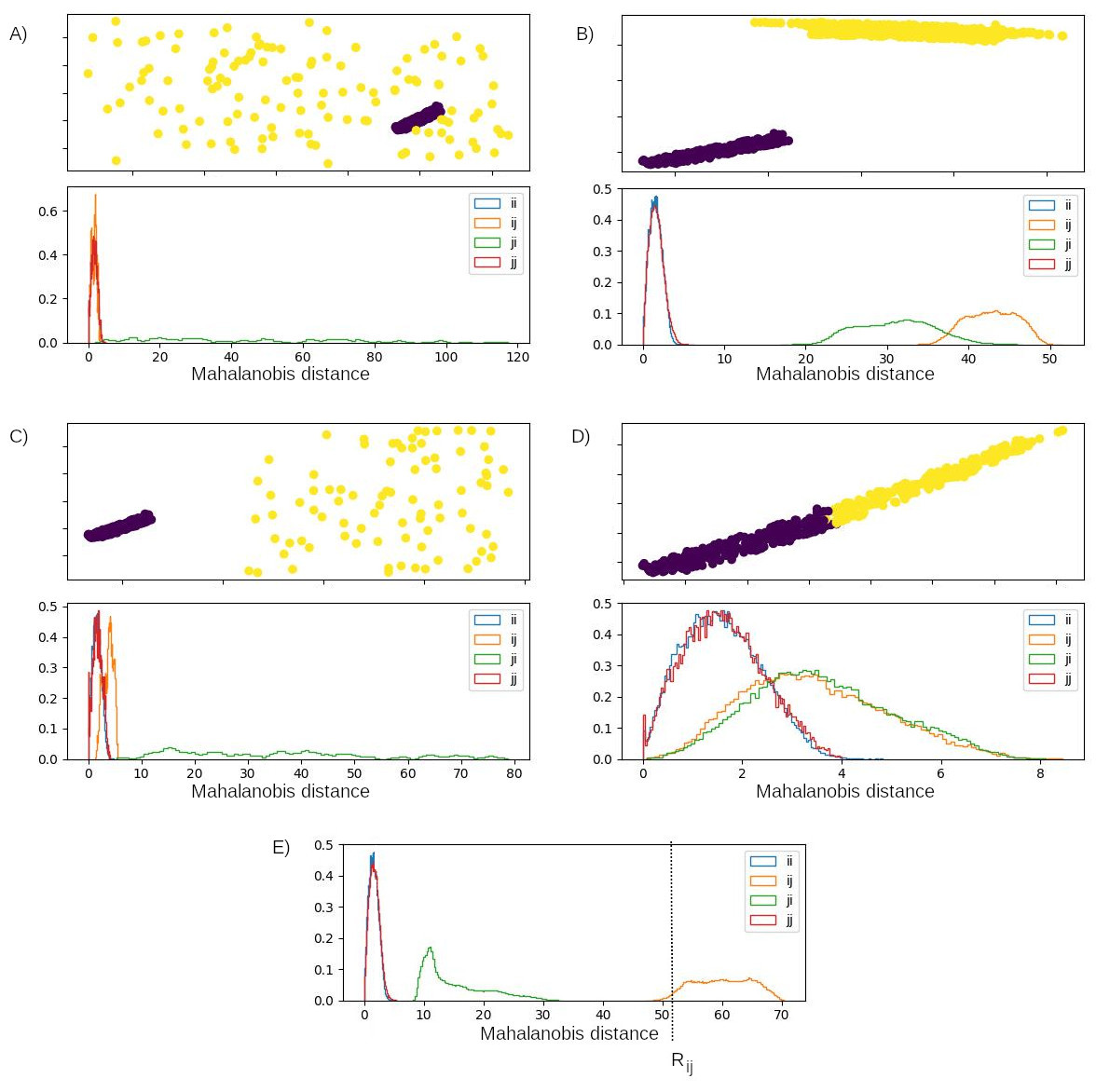
Figure 2: A-D) Distributions of points within clusters (different colors correspond to different clusters) and distributions of Mahalanobis distances corresponding to them (orange and green correspond to distributions of intercluster distances $p_{ij},p_{ji}$, red and blue correspond to cluster size distributions $p_{ii},p_{jj}$). E) An illustration of determining the intercluster distance $R_{ij}$ from the distributions of Mahalanobis distances for two clusters.

2.4 Stage 3: Grouping clusters into superclusters

DBSCAN was used as an algorithm for grouping the clusters into superclusters, matrix of intercluster distances $R_{ij}$ 8 is used as inter-object distances. To simplify the enumeration of the iterations over the maximal element distance in the supercluster $\varepsilon$, the DBSCAN $\varepsilon$ hyperparameter is used as iteration identifier. To do this all unique values of $\varepsilon$ were ordered in increasing order, and intermediate values

$$\overline{\varepsilon}_{k}=(\varepsilon_{k-1}+\varepsilon_{k})/2;\varepsilon_{0}=0$$ (9)

between the neighbors of this sequence were calculated. The resulting sequence of $\overline{\varepsilon}_{k}$ is used as iteration indices. Obviously, at the smallest distance $\overline{\varepsilon}_{1}$ DBSCAN produces the maximum possible value of clusters $N_{BIC}$ (determined from the optimality of the BIC criterion at the first stage of the algorithm), and at the largest $\overline{\varepsilon}_{k_{max}}$ DBSCAN produces only one cluster. In order to speed up algorithm, if iterating over 10 consecutive values of $\overline{\varepsilon}_{k}$ DBSCAN produces the number of clusters equal to 1, the iteration process over $\overline{\varepsilon}_{k}$ is stopped.

Further calculations of stop criteria require a matrix of distances between new superclusters $D_{ij}(\overline{\varepsilon})$. The distance $D_{SC_{i},SC_{j}}(\overline{\varepsilon})$ between two superclusters $SC_{i},SC_{j}$ is taken to be the minimum distance between clusters $C_{n},C_{m}$ belonging to these two superclusters :

$$D_{SC_{i},SC_{j}}(\overline{\varepsilon})=Min_{m,n:C_{m}\subseteq SC_{i},C_{n}\subseteq SC_{j}}(R_{mn})$$ (10)

In terms of speed, this algorithm is intermediate between a greedy algorithm (for example, agglomerative) and an exhaustive search. At the same time, at each iteration of $\overline{\varepsilon}$, it accurately estimates the number of superclusters produced by this solution. It should be noted that despite the fact that the DBSCAN method is a metric method, the used distance matrix $R_{ij}$ (defined in the previous step) is essentially a set of t-statistic values. Therefore, when performing this stage, we cluster the differences in the statistical characteristics of clusters, rather than their Cartesian characteristics.

2.5 Stage 4: Stop criteria

An important task is the choice of the optimal superclusters configuration and their number, which is reduced to the choice of the optimality criterion. It is obvious that new use of the BIC criterion will not bring any sufficient results: according to this criterion, we have already chosen the maximum number of clusters $N_{BIC}$. The other widely used criterion is the Silhouette criterion. However, it has a problem - it is related with the concept of subtracting distances (and hence connected with the Euclidean metric), which makes its statistical interpretation difficult, when distances are t-statistics. Therefore, we introduce a more clear criterion from statistical point of view - the matrix quality criterion (MC).

Let us formulate the problem of proximity of two clusters in terms of testing hypothesis. The null hypothesis is that $i,j$ clusters are close and the minimal distance $D_{ij}$ between them is statistically insignificant and statistically corresponds to the distances within single cluster. Alternative hypothesis that they are far from each other. Let us use the intercluster distance $D_{ij}$ as statistics for the testing this hypothesis. The distribution of distances $p_{ii}$ between points within a single gaussian cluster is the distribution of this statistics when null hypothesis is true.

One-sided $\alpha$-level statistical test for this criteria will be:

$$p_{value}(D_{ij})<\alpha$$ (11)

where $p_{value}$ is calculated over null-hypothesis distribution (i.e. over $p_{ii}$ distribution)

For Mahalanobis distance $p_{ii}$, the $p_{ii}^{2}/2$ value has $\chi^{2}$ distribution:

$$p_{ii}^{2}/2\sim\chi^{2}(N_{X})$$ (12)

where degrees of freedom $N_{X}$ is the dimension of the clustered points.

Due to for one-sided test $p_{value}(D)$ decreases with D increasing, the null hypothesis rejecting rule (11) can be rewriten in form:

$$D_{ij}(\overline{\varepsilon}_{k})>\delta D_{\alpha}$$ (13)

where

$$\delta D_{\alpha}=\sqrt{2\cdot Q_{1-\alpha}}$$ (14)

following (12), and calculated from quantile value $Q_{p}$ of $\chi^{2}(N_{X})$ distribution with given significance level $\alpha$ and known degrees of freedom $N_{X}$.

Following this rule the superclusters i-th and j-th are close (the null hypothesis can not be rejected) when condition (13) is not met. In this case the number of superclusters can be reduced by making next iteration $\overline{\varepsilon}_{k+1}$.

This hypothesis testing rule (11) can be interpreted in terms of Mahalanobis distance (13) by the following: if two superclusters are located at a distance $D_{ij}(\overline{\varepsilon})$ less than $\delta D_{\alpha}$, they can be considered close with a significance level $\alpha$. Therefore, as a matrix quality criterion (MC), we use the proportion of superclusters that do not have close superclusters:

$$MC(\overline{\varepsilon})=\frac{\sum_{i\in[1..N_{S}]}[Min_{j,j\neq i}(D_{ij}(\overline{\varepsilon}))>\delta D_{\alpha}]}{N_{S}(\overline{\varepsilon})}$$ (15)

where [x] is 1 when condition x is met, 0 otherwise, $N_{S}(\overline{\varepsilon})$ is a current number of superclusters (dimension of $D_{ij}$) at stage $\overline{\varepsilon}$.

For each supercluster, we determine whether the supercluster closest to it is separable from it or not. We divide the resulting number of separable superclusters by the total number of superclusters.

If we transfer all the distances $D_{ij}$ to p-values using (14), the MC criterion will become:

$$MC(\overline{\varepsilon})=\frac{\sum_{i\in[1..N_{S}]}[Max_{j\neq i}(p_{value}(D_{ij}(\overline{\varepsilon})))<\alpha]}{N_{S}(\overline{\varepsilon})}$$ (16)

and has clear statistical interpretation: maximal value 1 of this criterion demonstrates that every supercluster at stage $\overline{\varepsilon}$ is separated from others with significance level at least $\alpha$.

Obviously, $MC(\overline{\varepsilon})$ lies within $[0..1]$, and reaches its maximum value of 1 when we find the clustering where all superclusters are statistically significant separable from each other with significance level $\alpha$. The MC criteria do not depend on cluster sizes due to the sizes are similar and theoreticaly predicted from $\chi^{2}$ distribution (12).

Figure 3A-B shows dependence of MC criteria on iteration number and number of superclusters. Figure 3C-J shows the shapes of superclusters tested during training. The Figure 3A-B demonstrates the need to stop at the $\overline{\varepsilon}$ stage, at which $MC(\overline{\varepsilon})$ becomes 1 : after this the number of superclusters only decreases, and the value of the $MC(\overline{\varepsilon})$ criterion does not change. From the example shown in the figure, it can be seen that for the first time MC reaches the value of 1 at the 41th iteration, which leads to the splitting of the data set into 4 superclusters we expected - three nested rings and a noise. Further iterations do not improve the clustering, and leave MC unchanged.

Figure 3: Dependence of the MC (A), number of superclusters (B) and superclustering during training (C-K) as function of iteration number using ’three nested rings with noise’ data set as an example for $\alpha=0.1$.

3 Final algorithm

The final GMSDB algorithm consists of the following actions:

1. Get data set of $N_{X}$-dimension points $\overrightarrow{X}$;

2. For each number of clusters $N$ in given range (from 2 to a large enough number) make Gaussian Mixture clusterization of $\overrightarrow{X}$ - find parameters in eq.(4);

3. Find number of clusters $N_{BIC}$ for which the BIC is minimal and use corresponding optimal GM clusterization ($C_{m}$) of $\overrightarrow{X}$ for the following steps;

4. Calculate the cluster distance matrix $R_{mn}$ using each pair of found clusters $C_{m},C_{n}$, all their points pairs:

   $$\overrightarrow{x_{m}},\overrightarrow{y_{n}}\in\overrightarrow{X}:\overrightarrow{x_{m}}\in C_{m},\overrightarrow{y_{n}}\in C_{n}$$

   , eqs.(6, 8), and covariance matrices $S_{m},S_{n}$ for these clusters obtained at the previous step;

5. Get ordered sequence of unique distances $\varepsilon_{k}\in R_{mn},m\neq n,\varepsilon_{k}>0$, calculate $\overline{\varepsilon}_{k}$ using eq.(9);

6. For each $\overline{\varepsilon}_{k}$ from its smallest to its largest value do the following:

   1. Cluster the objects (clusters $C_{m}$), defined by the distance matrix $R_{mn}$ into the groups (superclusters $SC_{j}$) by DBSCAN method with its hyperparameter $\varepsilon=\overline{\varepsilon}_{k}$, get the number of found superclusters $N_{S}$;

   2. Calculate the supercluster distance matrix $D_{ij}$ between found superclusters $SC_{i},SC_{j}$ using eq.(10) and cluster distance matrix $R_{mn}$, calculated at step 4;

   3. Calculate MC from $D_{ij}$ using eq.(15,14), given data dimension $N_{X}$, number of found superclusters $N_{S}$, and given significance level $\alpha$ (default value $\alpha=0.1$);

   4. If MC is equal to 1 - exit the cycle;

7. Return found superclusters $SC_{j}$ as the solution.

4 Experiments

At first we test the algorithm in noise-free situations. The algorithm was tested on artificial data sets, the code of which is given in [2]. Some of these data sets are identical to those used for sklearn library [8] clustering tests (https://scikit-learn.org/stable/modules/clustering.html). All the data sets were generated by various transformations from a normal and uniform distributions, so data sets have varying cluster shapes and point densities within clusters.

Figure 4 shows the results of such testing. The ’three grains’ (Figure 4A), large (Figure 4B) and small (Figure 4C) ’blobs’, which are useful for testing clustering with statistical models and models based on centroids and distances between them; ’three horseshoes’ (Figure 4D) and ’two horseshoes’ (Figure 4E), which are useful for testing clustering with distance-based models, and ’three nested rings’ (Figure 4F) and ’two nested rings’ (Figure 4G).

The results of the GMSDB algorithm and the Agglomerative algorithm [17] was compared in the following way. The maximum possible number of clusters is 35, which exceeds $N_{BIC}$ for any data set. For agglomerative clustering, the distance is Euclidean, and the distance between clusters is calculated by their nearest elements.

The figure shows that in the case of well-separated ’grains’ (Figure 4A) and ’small blobs’ (Figure 4C) the algorithms work very similarly and the results are the same as expected - 3 and 5 main classes correspondingly. It can be seen that the agglomerative algorithm leaves artifacts on the cluster boundaries. The GMSDB algorithm produces no artifacts, and accurately guesses the number of superclusters. A similar situation occurs in the case of ’three horseshoes’ and ’two horseshoes’ (Figure 4D,E) - agglomerative clustering guesses the main body of the cluster quite well, but the edges with clustering artifacts become even larger. The GMSDB algorithm continues to correctly guess the number and shape of superclusters. ’Big blobs’ (Figure 4B), where the distance between clusters is of the order of their size, is problematic for both algorithms, but GMSDB guesses a little closer than the agglomerative one. The biggest difference is in ’three nested rings’ and ’two nested rings’ (Figure 4F,G) - the agglomerative one cannot adequately separate them - as the radius increases (and the density of points decreases), the ring is divided into an increasing number of clusters. Unlike the agglomerative algorithm, GMSDB adequately clusterizes these data sets.

Figure 4: Comparison of clustering of different identical data sets by GMSDB and agglomerative algorithms (minimal interobject distance as intercluster distance, metric - euclidean). Noise-free situation. The maximum allowed number of clusters is 50, $\alpha=0.1$. From left to right - the original data set, clustering by the GMSDB algorithm and the found optimal number of superclusters, decision regions of the trained GMSDB algorithm, clustering by the agglomerative algorithm. Bottom left corner in second column images - the number of superclusters detected by GMSDB.

Examples of testing at noisy data sets are shown in Figure 5. Here the situation is much different. The impact of noise on ’middle blobs’ clustering (Figure 5A) makes classification more difficult with the agglomerative method, but still allows clustering with the GMSDB algorithm.

The last test is ’two snakes’ (Figure 5E) - the result of the t-SNE transform [19] of the ’two noisy horseshoes’ data set (Figure 5B). Two snakes - a data set of two clusters and noise, which has a complex shape and an inhomogeneous noise-like structure inside and outside clusters. The distances between two clusters in different regions are different and comparable with the characteristic sizes of the clusters themselves. This data set cannot be adequately clustered by both algorithms (agglomerative and GMSDB), but it can be easily seen that the GMSDB algorithm finds fewer superclusters than the agglomerative algorithm and detects two largest superclusters corresponding to ’snakes’ sufficiently well.

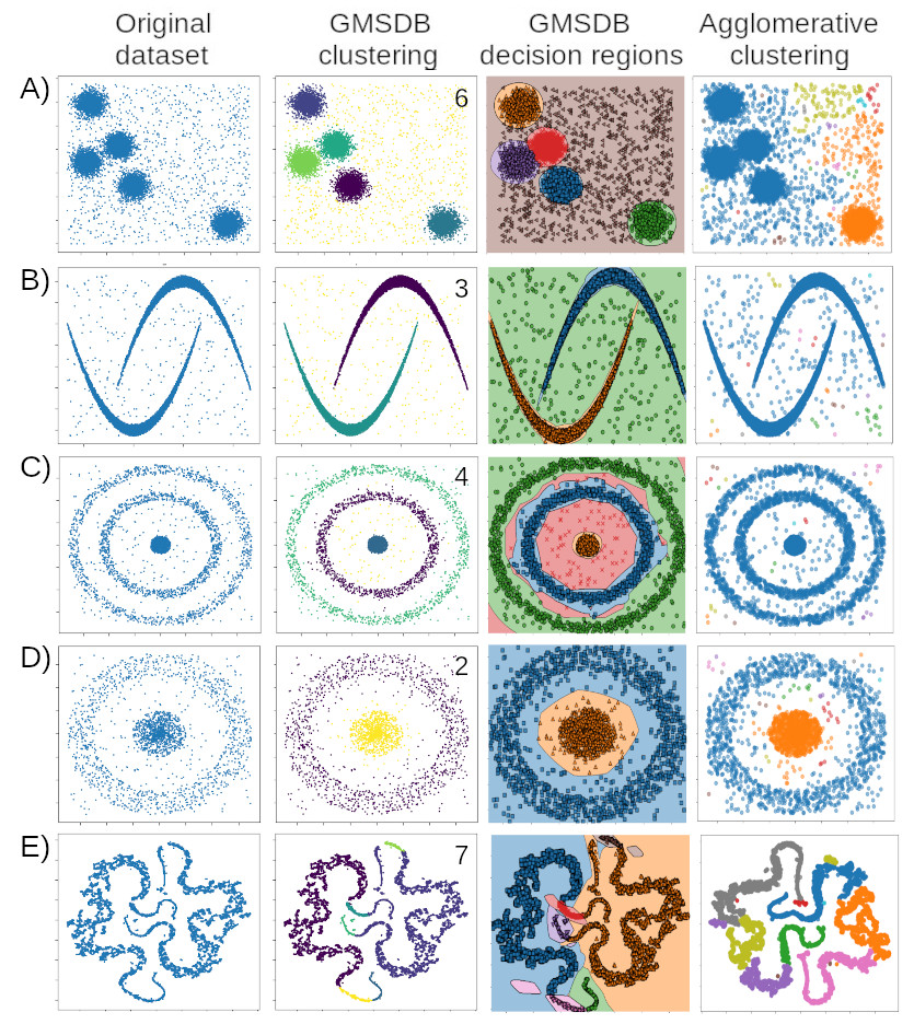
Figure 5: Comparison of clustering of different identical data sets by GMSDB and agglomerative algorithms (minimal interobject distance as intercluster distance, metric - euclidean). Noisy situation. The maximum allowed number of clusters is 50, $\alpha=0.1$. From left to right - the original data set, superclustering by the GMSDB algorithm and the found optimal number of superclusters, decision regions of the trained GMSDB algorithm, clustering by the agglomerative algorithm. Top right corner in second column images - the number of superclusters detected by GMSDB.

5 Discussion

According to Kleinberg’s impossibility theorem [4], there is no clustering algorithm that is simultaneously scale-invariant, consistent, and rich. Obviously, the proposed GMSDB algorithm is unrich - it does not enumerate all clustering/superclustering variants. Let us evaluate how it differs from the rich one in order to understand what possible clusterings it is limited to. Obviously, if the number of Gaussian distributions is equal to the number of points in the data set, then the algorithm ’find the parameters of all Gaussian distributions, and then combine them to obtain a clustering labeled by expert’ is almost rich - for discrete points (we usually work with such data sets), it is enough to choose Gaussian distributions much narrower than the minimum distance between points. Compared to the full algorithm in the GMSDB algorithm we limit the number of normal distributions and their shape: their shape is determined from the EM algorithm by the maximum likelihood condition, and the number is determined from the minimum of the BIC criterion. The possible combinations of clusters (superclusters) in the GMSDB algorithm are also limited - there should be the maximum number of superclusters separable by the Mahalanobis distance with a significance level $\alpha$. This limits the set of possible clusterings that the algorithm is able to determine adequately. In practice, it is not able to correctly separate non-connected or significantly overlapping clusters, as well as clusters in which there are not enough elements for the EM algorithm to work or which are ’not likelihood enough’, and could be clustered by different way with more likelihood in terms of Gaussian Mixture.

The high quality of the algorithm is demonstrated in noiseless (Figure 4) and noisy (Figure 5) situations compared to the agglomerative algorithm.

The advantages of the GMSDB method include also its statistical formulation, which makes it possible to estimate the probabilities of points belonging to a particular supercluster, and use it to classify new data both in the hard clustering mode and in the soft (fuzzy) clustering mode. Indeed, it is known that a mixture of Gaussians is capable to produce soft clustering - to estimate for each point the probability of its belonging $P_{C_{j}}(\overrightarrow{x})$ to one or another Gaussian cluster $C_{j}$. Each supercluster $SC_{i}$ is a union of the original Gaussian clusters and the sets of clusters in different superclusters do not intersect. So the probabilities of any new point belonging to supercluster $P_{SC_{i}}(\overrightarrow{x})$ can be calculated from the probabilities of belonging this point to the clusters $C_{j}\subseteq SC_{i}$ that form this supercluster:

$$P_{SC_{i}}(\overrightarrow{x})=\sum_{j:C_{j}\subseteq SC_{i}}P_{C_{j}}(\overrightarrow{x})$$ (17)

Table 1 shows the average time of clustering data sets by the GMSDB and Agglomerative algorithms (in seconds, by an identical computer), as well as the Rand Index (RI) confidential interval over 10 runs, determined from the initial labeling of the test data sets during their creation. In noisy cases, noise was marked as a separate class.

From Table 1 it can be seen that the GMSDB algorithm is most often more adequate than the agglomerative algorithm, especially on noise-free data sets. Higher RI values indicate higher adequacy.

The main disadvantage of the algorithm is its speed, shown in Table 1. It can be seen from the table that GMSDB is two orders of magnitude slower than the agglomerative algorithm, so its use is recommended when one takes into account its low speed, in the case when the adequacy of clustering is very important, and there is much enough data for its operation. The algorithm is implemented in Python, so using fast search algorithms or other programming languages for these tasks could improve its performance. Its current variant [2] has implementations for the speed optimization by a kind of dichotomy search for stage 1 and Monte-Carlo search for stage 3, significantly improving clustering speed.

Table 1: The execution time for clustering identical data sets by the GMSDB and Agglomerative algorithms (in seconds), as well as the Rand Index (RI) determined from the initial labeling of test data sets during their creation (in noisy cases, noise is marked as a separate class). Bold indicates the best RI result for given data set.

	GMSDB					Agglomerative
data set	St.1	St.2	St.3,4	Tot.time	RI interval (0.95)	time	RI interval (0.95)
Noise-free data sets (Figure 4)
Grains	10.0	21.7	0.02	32.0	1.0	0.67	0.998
Big blobs	9.7	14.6	0.01	24.3	0.76	0.62	0.52
Small blobs	11.1	14.4	0.01	25.5	1.0	0.60	0.999
3 horseshoes	17.6	44.0	0.04	61.6	1.0	1.6	0.987
2 horseshoes	19.5	20.0	0.02	39.5	1.0	0.68	0.975
3 nested rings	3.4	3.5	0.04	6.9	1.0	0.08	0.9
2 nested rings	1.0	0.7	0.04	1.7	1.0	0.046	0.825
Noisy data sets (Figure 5)
Medium blobs	10.6	21.3	0.02	31.9	0.985..0.988	0.78	0.18..0.51
2 horseshoes	17.6	21.2	0.1	38.8	0.994..0.996	0.66	0.48..0.49
3 nested rings	5.6	3.4	0.1	9.1	0.942..0.955	0.09	0.30..0.72
2 nested rings	2.6	1.2	0.01	3.8	0.880..0.883	0.059	0.42..0.89
2 snakes	17.5	19.2	0.4	37.1	0.72..0.83	0.71	0.65..0.85

The next drawback is the presence of a control hyperparameter - the significance level $\alpha$. To obtain all the results described above, we used $\alpha=0.1$, exceeding standard statistical value 0.05.

The last disadvantage of the method is the stochasticity of the results - the optimal separation of the same data set can change from run to run. This is due to the algorithm is based on the EM implementation of GM, which is based on an iterative algorithm and depends on the initial conditions. Examples and their probabilities are shown in Figure 6.

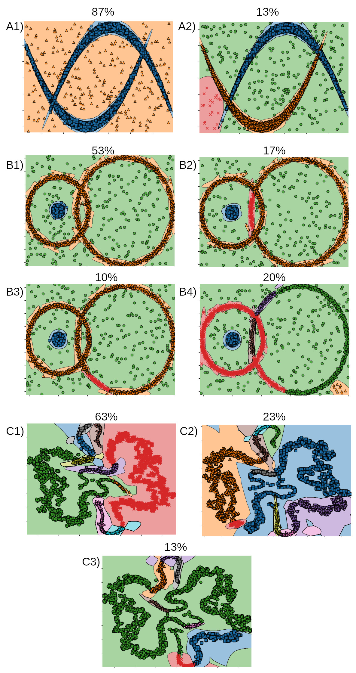
Figure 6: The effect of stochasticity to clustering in the case of intersecting clusters and the probability of occurrence of these cases over 30 runs (top). A1-A2) two intersecting horseshoes, B1-B4) intersecting rings, C1-C3) two snakes

6 Conclusion

The paper presents a statistical algorithm for GMSDB adequate clustering a data set by an optimal grouping of inadequate gaussian models.

The algorithm performs two sequential operations - approximates the set of points under study by the optimal superposition of normal distributions, each of them, taken separately, is generally not an adequate cluster in the data. To create a model of adequate clusters, the algorithm groups the resulting Gaussian distributions into the maximum number of separable superclusters (with given statistical significance level $\alpha=0.1$). Thus, the algorithm clusters the data set into statistically separated superclusters, each of which is described by a superposition of normal distributions.

The algorithm consists of three main stages: approximates the data set by a mixture of Gaussian distributions, the number of which is determined based on the minimum of the BIC criterion; uses the Mahalanobis distance for estimating the statistical distances between clusters and cluster sizes; combines the resulting clusters into superclusters using the DBSCAN method by sequential iterations over its hyperparameter (maximum distance $\varepsilon$) from smaller to larger values; stops the iterations over the hyperparameter when the matrix quality criterion MC introduced by us reaches its maximum value of 1. The matrix quality criterion calculates the proportion of statistically significant separable superclusters among all found superclusters. Therefore the algorithm joins hierarchical and partitional methods into a single scheme based on statistical theory testing approach.

Although the algorithm is computationally very slow, it shows good results on several test data sets, in noise and noiseless situations. An essential advantages of the method are: the ability to predict a cluster for new data based on an already trained clusterer, and the possibility of soft (fuzzy) clustering. The Python source code of the clusterer is available in [2] and available at PyPI as gmsdb package.

References

- [1] D. Arthur and S. Vassilvitskii. K-Means++: The Advantages of Careful Seeding. In Proceedings of the Eighteenth Annual ACM-SIAM Symposium on Discrete Algorithms, SODA ’07, pages 1027–1035, USA, 2007. Society for Industrial and Applied Mathematics.
- [2] O. Berngardt. berng/gmsdb, 2023.
- [3] M. Ester, H.-P. Kriegel, J. Sander, and X. Xu. A Density-Based Algorithm for Discovering Clusters in Large Spatial Databases with Noise. In Proceedings of the Second International Conference on Knowledge Discovery and Data Mining, KDD’96, pages 226–231. AAAI Press, 1996.
- [4] J. Kleinberg. An Impossibility Theorem for Clustering. In Proceedings of the 15th International Conference on Neural Information Processing Systems, NIPS’02, pages 463–470, Cambridge, MA, USA, 2002. MIT Press.
- [5] P. Mahalanobis. On the Generalised Distance in Statistics. Proceedings of the National Institute of Sciences of India, 2(1):49–55, 1936.
- [6] G. J. McLachlan. Discriminant Analysis and Statistical Pattern Recognition. Wiley, 1992.
- [7] A. Ng, M. Jordan, and Y. Weiss. On Spectral Clustering: Analysis and an algorithm. In T. Dietterich, S. Becker, and Z. Ghahramani, editors, Advances in Neural Information Processing Systems, volume 14. MIT Press, 2001.
- [8] F. Pedregosa, G. Varoquaux, A. Gramfort, V. Michel, B. Thirion, O. Grisel, M. Blondel, P. Prettenhofer, R. Weiss, V. Dubourg, J. Vanderplas, A. Passos, D. Cournapeau, M. Brucher, M. Perrot, and E. Duchesnay. Scikit-learn: Machine learning in Python. Journal of Machine Learning Research, 12:2825–2830, 2011.
- [9] W. M. Rand. Objective Criteria for the Evaluation of Clustering Methods. Journal of the American Statistical Association, 66(336):846–850, 1971.
- [10] L. A. Rasyid and S. Andayani. Review on Clustering Algorithms Based on Data Type: Towards the Method for Data Combined of Numeric-Fuzzy Linguistics. Journal of Physics: Conference Series, 1097(1):012082, sep 2018.
- [11] D. Reynolds. Gaussian Mixture Models, pages 827–832. Springer US, Boston, MA, 2015.
- [12] M. Z. Rodriguez, C. H. Comin, D. Casanova, O. M. Bruno, D. R. Amancio, L. da F. Costa, and F. A. Rodrigues. Clustering algorithms: A comparative approach. PLOS ONE, 14(1):e0210236, jan 2019.
- [13] A. Saxena, M. Prasad, A. Gupta, N. Bharill, O. P. Patel, A. Tiwari, M. J. Er, W. Ding, and C.-T. Lin. A review of clustering techniques and developments. Neurocomputing, 267:664–681, dec 2017.
- [14] E. Schubert, J. Sander, M. Ester, H. P. Kriegel, and X. Xu. DBSCAN Revisited, Revisited: Why and How You Should (Still) Use DBSCAN. ACM Trans. Database Syst., 42(3), jul 2017.
- [15] G. Schwarz. Estimating the Dimension of a Model. The Annals of Statistics, 6(2):461 – 464, 1978.
- [16] X. Shiming, N. Feiping, and Z. Changshui. Learning a Mahalanobis distance metric for data clustering and classification. Pattern Recognition, 41(12):3600–3612, 2008.
- [17] R. Sibson. SLINK: An optimally efficient algorithm for the single-link cluster method. The Computer Journal, 16(1):30–34, 01 1973.
- [18] Student. The probable error of a mean. Biometrika, 6(1):1, mar 1908.
- [19] L. van der Maaten and G. Hinton. Visualizing Data using t-SNE. Journal of Machine Learning Research, 9(86):2579–2605, 2008.