Testing Meson Portal Dark Sector Solutions to the MiniBooNE Anomaly at CCM

Abstract

A solution to the MiniBooNE excess invoking rare three-body decays of the charged pions and kaons to new states in the MeV mass scale was recently proposed as a dark-sector explanation. This class of solution illuminates the fact that, while the charged pions were focused in the target-mode run, their decay products were isotropically suppressed in the beam-dump-mode run in which no excess was observed. This suggests a new physics solution correlated to the mesonic sector. We investigate an extended set of phenomenological models that can explain the MiniBooNE excess as a dark sector solution, utilizing long-lived particles that might be produced in the three-body decays of the charged mesons and the two-body anomalous decays of the neutral mesons. Over a broad set of interactions with the long-lived particles, we show that these scenarios can be compatible with constraints from LSND, KARMEN, and MicroBooNE, and evaluate the sensitivity of the ongoing and future data taken by the Coherent CAPTAIN Mills experiment (CCM) to a potential discovery in this parameter space.

I Introduction

The excess of electron-like events observed by MiniBooNE Aguilar-Arevalo et al. (2009a, 2018a, 2021a) at a level of $4.8\sigma$ has remained one of the stronger hints to the existence of new physics beyond the Standard Model (SM). The event data observed in the MiniBooNE detector is remarkable for its spectrum, with the excess appearing at forward scattering angles ($\cos\theta>0.75$) and low energies ($E_{vis}<500$ MeV), and for the asymmetry of excess events in the neutrino and anti-neutrino modes, while no excess was observed in the dump mode Aguilar-Arevalo et al. (2018b), which had a reduced neutrino flux.

Neutrino-based new physics explanations have been popular solutions to the anomaly Sorel et al. (2004); Karagiorgi et al. (2009); Collin et al. (2016); Giunti and Laveder (2011a, b); Gariazzo et al. (2017); Böser et al. (2020); Kopp et al. (2011, 2013); Dentler et al. (2018); Abazajian et al. (2012); Conrad et al. (2013); Diaz et al. (2020); Asaadi et al. (2018); Karagiorgi et al. (2012); Pas et al. (2005); Döring et al. (2020); Kostelecky and Mewes (2004); Katori et al. (2006); Diaz and Kostelecky (2011, 2012); Gninenko (2009); Gninenko and Gorbunov (2010); Bai et al. (2016); Moss et al. (2018); Bertuzzo et al. (2018); Ballett et al. (2019); Fischer et al. (2020); Moulai et al. (2020); Dentler et al. (2020); de Gouvêa et al. (2020); Datta et al. (2020); Dutta et al. (2020); Abdallah et al. (2020); Abdullahi et al. (2021); Liao and Marfatia (2016); Carena et al. (2017); Abdallah et al. (2021). Since the neutrinos at MiniBooNE are produced primarily from charged meson decays and the decays of daughter muons of those charged mesons, neutrino-based solutions can accommodate the absence of any excess in the dump mode, in which the charged mesons are no longer focused by magnetic horns, unlike the neutrino and anti-neutrino modes. Essentially, the neutrino-based explanations work well because a key feature of the excess seems to be correlated to the focusing or suppression of charged mesons. Further, since the energy and angular distributions of the excess are already characteristic of neutrino-like signals and backgrounds, new physics appearing in the neutrino sector may naturally map onto the observed spectra.

This poses a challenge to dark sector interpretations of the excess (e.g., using $\pi^{0}$ or dark bremsstrahlung production channels Aguilar-Arevalo et al. (2018b); Jordan et al. (2019)), which have been more constrained and less complete in their explanation of the excess with respect to their counterparts in neutrino BSM physics thus far. Recently, a generic set of solutions to the excess was proposed in ref. Dutta et al. (2021) using a framework of rare three-body decays of the charged mesons – decays which may not be strongly suppressed in their phase space and can be powerful probes of BSM physics Barger et al. (2012); Carlson and Rislow (2012); Laha et al. (2014); Bakhti and Farzan (2017); Altmannshofer et al. (2020); Krnjaic et al. (2020). One subset of models considered consists of a long-lived dark sector boson (not necessarily the cosmological DM, but at least long-lived on the scale of the BNB-to-MiniBooNE beamline of $\sim 500$m) that can survive and scatter in the MiniBooNE detector via a photoconversion process, leaving a single photon in the final state. Since the Cherenkov detector does not distinguish between photons and electrons, this scattering process can be a viable contributor to the excess, provided that the appropriate phenomenological model can be found to be safe from existing constraints.

In this work, we will constrain the space of operators in an effective field theory (EFT) that leads to rare three-body decays of the charged mesons and photoconversion scattering of long-lived mediators at Coherent CAPTAIN Mills (CCM), utilizing the close proximity to the Lujan beam target as a source of stopped-pion decays. Using the CCM120 engineering run, we set conservative limits on the parameter space, and forecast sensitivity for the ongoing 3-year run with the upgraded CCM200 detector. A similar analysis for electromagnetic signal region of interest (ROI) that was performed for axion-like particles in ref. Aguilar-Arevalo et al. (2023) is carried out here. In surveying the greater landscape of dark sector models that can explain the MiniBooNE anomaly via rare meson decays, we also take into account the analyses and observations from other stopped-pion experiments like LSND and KARMEN. Important findings about the parameter space that we consider here can be distilled from the existing data at MicroBooNE, and other forthcoming short-baseline experiments like SBND have a discovery potential here as we will show. In fact, the joint analysis of close-proximity stopped-pion experiments and those at the short-baseline neutrino program with magnetic horn-focused charged meson fluxes will have total experimental coverage over the parameter space explaining the anomaly.

This paper is organized as follows. In § II we introduce the operator EFT extension to the SM that we wish to consider and connect it to a phenomenological model of pion decays and photoconversion scattering in § III. In § IV the analysis procedures for both MiniBooNE target and dump mode runs is discussed, in addition to our analysis of LSND, KARMEN, and MicroBooNE data interpreted as constraints on the models in question. In § V we show the analysis procedure for the CCM120 engineering run data and construct forecasts for the ongoing CCM200 data-taking run. In § VI the resulting fits and constraints are shown for several benchmark models that utilize the operators we have considered in § II, and finally in § VII we conclude.

II Models

We study a set of effective operators which permit, at a purely phenomenological level, the production of a long-lived particle (LLP) bosonic state from the three-body decay of the charged mesons, and subsequent photoconversion of said meson via a massive mediator; schematically,

$$\underbrace{\leavevmode\hbox to0pt{\vbox to0pt{\text{[drawing]}}}}_{\textrm{Beam Target Production}}\leavevmode\hbox to0pt{\vbox to0pt{\text{[drawing]}}}\underbrace{\leavevmode\hbox to0pt{\vbox to0pt{\text{[drawing]}}}}_{\textrm{Detection}} \pi^{\pm} X \nu \ell + X \gamma N N Y \pi^{\pm} X \nu \ell + X \gamma N N Y$$

This simple setup was shown to explain the MiniBooNE excess in ref. Dutta et al. (2021), making use of two prominant features; (I) the coupling of a boson $X$ to the charged pion decays ensures the $X$ flux is correlated to the relative size of the excess in the target and off-target modes through the focusing of charged pions via the magnetic horns, and (II) the mass of the mediator $Y$ gives a dial to tune the angular spectrum of the outgoing $\gamma$’s Cherenkov ring, which is characteristically off-forward.

We will investigate a broad set of operators that allow for such a phenomenology in order to estimate the relative sizes of the parameter space allowed by existing constraints that also can accomodate the MiniBooNE excess. In §. II.1 we consider a generic EFT for the two bosons $X$ and $Y$ below the QCD scale, while in §. II.2 we consider a hadrophillic scenario with a single new boson and connect the EFT to specific quark couplings above the QCD scale.

II.1 One Long-lived Boson and a Secondary Massive Mediator

We study two BSM scenarios that each could explain the MiniBooNE excess and are testable at stopped pion and other beam dump facilities. In the first scenario, we extend the low energy SM EFT with two massive bosons, one of them long-lived and being produced via the three-body decay of the charged mesons and the other generally being heavier and facilitating photoconversion $XN\to\gamma N$. These decay and scattering mechanisms can arise from a multitude of operators. For the decays, scalars ($\phi$), pseudoscalars ($a$), or vectors ($V$) coupled to the electrons or muons through $g_{\ell}^{s}\phi\bar{\ell}\ell$, $-ig_{\ell}^{p}a\bar{\ell}\gamma^{5}\ell$, and $g_{\ell}^{V}V_{\mu}\bar{\ell}\gamma^{\mu}\ell$ terms allow for $\pi^{\pm}\to X\ell\nu$ where $X=\phi,a,V$ is radiated off the charged lepton leg. Alternatively, effective couplings to the charged pions through operators like $g^{s}_{\pi}\phi\pi^{+}\pi^{-}$ or $g^{v}_{\pi}V_{\mu}\pi^{+}(\partial^{\mu}\pi^{-})$ allow for radiative decays from the pion current (and potentially other contact and pion structure-dependent interactions, discussed in the next section).

On the detection side, the long-lived $\phi,a$, or $V$ mediators can induce single-photon final states through the dimension-5 couplings $\frac{\lambda^{s}}{4}\phi H_{\mu\nu}F^{\mu\nu}$ and $\frac{\lambda^{p}}{4}aH_{\mu\nu}\tilde{F}^{\mu\nu}$, where we define $H_{\mu\nu}\equiv\partial_{\mu}V_{\nu}-\partial_{\nu}V_{\mu}$. In these cases, either a vector, scalar, or pseudoscalar can serve as the long-lived $X$ and another as the scattering mediator $Y$. Such operators can arise easily in concrete, UV-complete models. For example, they can fit within the framework of a $U(1)$ extension to the SM with extra fermions that permit a loop-induced coupling between a (pseduo)scalar, the $U(1)$ gauge boson, and the SM photon (see e.g. $U(1)_{T3R}$ Dutta et al. (2022) models or dark photon / axion portals Kaneta et al. (2017)).

II.2 A Single Long-lived Boson Coupling to Quarks

For this scenario, we consider a hadrophillic model that only couples to first generation quarks. Let’s start with a massive vector boson, where above the QCD phase transition, its interactions with quarks is described by the Lagrangian

$$\mathcal{L} \supset\sum_{q=u,d}g_{q}V_{\mu}\overline{q}\gamma^{\mu}q+\textrm{h.c.}$$ (1)

We could interpret this as an extra $U(1)$ gauging the quarks with some dark charge, for example. Taking this below the QCD scale in the chiral perturbation theory ($\chi$PT), we have an operator like Berger et al. (2020)

$$\mathcal{L}^{\chi PT}\supset ig_{\pi^{\pm}}V_{\mu}\pi^{+}(\partial^{\mu}\pi^{-})$$ (2)

Additionally, the chiral anomaly will lead to the anomalous decay of the $\pi^{0}$ to $\gamma V$ through the dimension-5 operator

$$\mathcal{L}^{\chi PT}\supset g_{\pi^{0}}\frac{e}{16\pi f_{\pi}}\pi^{0}F_{\mu\nu}\tilde{H}^{\mu\nu}$$ (3)

We have defined $H_{\alpha\beta}=\partial_{\alpha}V_{\beta}-\partial_{\beta}V_{\alpha}$, and $\tilde{H}^{\mu\nu}=\epsilon^{\mu\nu\alpha\beta}H_{\alpha\beta}$. The dimension-5 interaction $\sim\pi^{0}F_{\mu\nu}\tilde{H}^{\mu\nu}$ permits $XN\to\gamma N$ via the pion-nucleon interaction $ig_{\pi N}\pi^{0}\bar{\psi}\gamma^{5}\psi$. This is an interaction of strong coupling; $g_{\pi N}\simeq 13$ de Swart et al. (1997).

III Phenomenology

III.1 Three-body Decays of Charged Mesons

Figure 1: 3-body charged meson decay $\pi\to\ell\nu X$ for a bosonic Lorentz representation $X=\phi,a,V$.

The three-body radiative decay of the $X$ boson off the pion current (Fig. 1) can be modeled off the work on radiative meson decays in the SM, like $\pi\to\gamma e\nu$ (see for example refs. Donoghue and Holstein (1989); Bryman et al. (1982)). For the process $\pi(p)\to X(k)e(\ell)\nu(q)$, there are several types of so-called “internal bremsstrahlung” (IB) interactions, adopting the nomenclature of the aforementioned reference; IB1, radiating $X$ off the lepton leg; IB2, radiating off the charged meson current; and IB3, or a 4-point contact interaction radiating off the pion-lepton vertex. Additionally, we may also consider structure-dependent (SD) terms originating from mixing between the new boson $X$ and the vector mesons, but as these branching ratios are strongly suppressed, we will set them aside in this discussion.

Our discussion now focuses on a massive vector boson $V$ taking part in these radiative decays, but we will return to the case of $X=$ scalar, pseudoscalar later.

The matrix elements for each process can be described by factorizing the leptonic and hadronic parts of the current;

$$\mathcal{M} =i\frac{G_{F}}{\sqrt{2}}\varepsilon^{\mu}\big{[}\bar{u}_{\ell}\gamma^{\rho}(1-\gamma^{5})v_{\nu}\big{]}T_{\mu\rho}$$ (4)

where the hadronic tensor $T_{\mu\rho}$ can be expressed in terms of the amplitude

$$T_{\mu\rho}=i\int d^{4}xe^{ikx}\braket{0}{T[j^{V}_{\mu}(x)j^{+}_{\rho}(0)]}{\pi^{+}(p)}$$ (5)

for currents $j^{V}_{\mu}=\sum_{q}g_{q}\bar{q}\gamma_{\mu}q$ and $j^{+}_{\rho}=\bar{d}\gamma_{\rho}(1-\gamma^{5})u$. The IB2 term shown in Fig. 1, middle, is given by

$$T_{\mu\rho}^{\textrm{IB2}}=\dfrac{i(2p-k)_{\mu}(p-k)_{\rho}}{2p\cdot k-m_{V}^{2}}f_{\pi}$$ (6)

which may come directly from the action in Eq. 2, $ig_{\pi^{\pm}}V_{\mu}\pi^{+}(\partial^{\mu}\pi^{-})$, while additional contact and structure-dependent terms in Fig. 1, bottom, may come from less trivial interactions. For example, a simple contact term could manifest from making the gauge covariant replacement $\partial_{\mu}\to\partial_{\mu}-ig_{\pi^{\pm}}V_{\mu}$ in the pion-lepton Fermi interaction $(\partial_{\mu}\pi^{+})\bar{\ell}\gamma^{\mu}(1-\gamma^{5})\nu$.

However, we can only speculate about the gauge nature of our massive vector, and so to proceed naively we decompose the hadronic tensor $T_{\mu\rho}$ in a gauge covariant way. We follow the approach given in ref. Khodjamirian and Wyler (2001), expressing $T_{\mu\rho}$ in terms of the momenta $k_{\mu}$ and $L_{\mu}\equiv q_{\mu}+\ell_{\mu}$;

$$T_{\mu\rho} =\tilde{a}_{0}g_{\mu\rho}+\tilde{b}_{0}L_{\mu}k_{\rho}+\tilde{b}_{1}L_{\rho}k_{\mu}$$

$$+\tilde{b}_{2}L_{\mu}L_{\rho}+\tilde{b}_{3}k_{\mu}k_{\rho}+\epsilon_{\rho\mu\lambda\sigma}L^{\lambda}k^{\sigma}F_{V}$$ (7)

where $\tilde{a}_{0}$, $\tilde{b}_{i}$ ($i=0,1,2,3$), and $F_{V}$ are dimensionful invariant amplitudes. For massless photons, satisfying the Ward identity imposes a relationship between the coefficients Khodjamirian and Wyler (2001); Beneke et al. (2018); Beneke and Rohrwild (2011); Bansal and Mahajan (2021). However, for a massive vector boson $V^{\mu}$, no Ward identity needs to be satisfied in general, as a theory with massive vector bosons need not be gauge invariant. Noting that $L\cdot k=(p-k)\cdot k$, the IB2 term in Eq. 6 is recovered if one takes $\tilde{b}_{2}=2\tilde{b}_{1}=if_{\pi}/(2L\cdot k+m_{V}^{2})$. The remaining terms $\tilde{a}_{0},\tilde{b}_{0}$, $\tilde{b}_{2}$ and $F_{V}$ account for contact and structure dependent contributions. For example, a pure contact term would take the form

$$T_{\mu\rho}^{\text{IB3}}=if_{\pi}\alpha g_{\mu\rho}+i\beta\frac{f_{\pi}}{(L\cdot k)}g_{\mu\rho}$$ (8)

for dimensionless constants $\alpha,\beta$. In this analysis we will consider only two instances of the meson couplings; those of IB2 nature (Fig. 1, middle, or Eq. 6) and those of a pure contact or IB3 nature (Fig. 1, bottom or Eq. 8).

III.2 Dark Boson Photoconversion

Long-lived bosonic states may have dimension-5 couplings between a secondary dark boson and the SM photon. This operator may arise e.g. at the 1-loop level from a theory connecting fermions charged under $U(1)_{em}$ to additional scalar and vector fields, or from the $\pi^{0}\gamma X$ vertex in our single-mediator, hadrophillic scenario at the $\chi PT$ level. This opens a scattering channel similar to axion photoconversion or Primakoff scattering, except instead of the SM photon being in the $t$-channel, the secondary massive boson takes its place. This process $XN\to\gamma N$ (see Fig. 2) may be coherent if the mediator for the scattering couples to nucleons, provided that the momentum transfer scale $q\lesssim 1/R_{n}$ for a nuclear size $R_{n}$ and that the sum of the neutron and proton charges coupled to the mediator is not small, so that the total amplitude picks up a coherent enhancement $\propto(\sum_{p}Q_{p}+\sum_{n}Q_{n})^{2}$. For simplicity we will assume that this coherent enhancement goes according to the proton number squared, $Z^{2}$, although depending on the baryonic couplings it could be as large as $A^{2}$, the nucleon number squared. In the case of scalar photoconversion on a nucleus of mass $M$ via a heavy vector mediator $V$, we have

$$\braket{}{\mathcal{M}}{{}^{2}}_{\textrm{V}}^{\phi\to\gamma} =(g_{n}\lambda^{s})^{2}t\big{[}2M^{2}(m_{\phi}^{2}-2s-t)+2M^{4}$$

$$-2m_{\phi}^{2}(s+t)+m_{\phi}^{4}+2s^{2}+2st+t^{2}\big{]}$$

$$\times\frac{F_{N}^{2}(t)}{(8(m_{V}^{2}-t)^{2})}$$ (9)

where $s,t$ are the Mandelstam invariants for the center of momentum energy and momentum transfer, respectively. The nuclear form factor $F_{N}^{2}(t)$, for which we take the well-known Helm parameterization with normalization $F_{N}^{2}(0)=Z^{2}$. The same matrix element holds in the case of pseudoscalar photoconversion $a\to\gamma$. For vector photoconversion via a heavy scalar or pseudoscalar mediator, the spin-averaged matrix elements are

$$\braket{}{\mathcal{M}}{{}^{2}}_{\textrm{S}}^{V\to\gamma} =\frac{3(g_{n}^{s}\lambda^{s})^{2}\left(4M^{2}-t\right)\left(m_{V}^{2}-t\right)^{2}}{16\left(m_{\phi}^{2}-t\right)^{2}}F_{N}^{2}(t)$$ (10)

$$\braket{}{\mathcal{M}}{{}^{2}}_{\textrm{P}}^{V\to\gamma} =\frac{(g_{n}^{p}\lambda^{p})^{2}\left(M^{2}-t\right)\left(m_{V}^{2}-t\right)^{2}}{8\left(m_{a}^{2}-t\right)^{2}}F_{N}^{2}(t)$$ (11)

Figure 2: Left: Vector photoconversion via a massive scalar or pseudoscalar mediator. Right: Scalar or pseudoscalar photoconversion via a massive vector mediator. Bottom: (pseudo)scalar dipole photoconversion.

The cross sections associated with these matrix elements are shown in Fig. 3. Notice that since in the case of an incoming vector photoconverting via a heavy scalar or pseudoscalar, $\braket{}{\mathcal{M}}{{}^{2}}_{\textrm{S,P}}^{V\to\gamma}$ has no $s$ dependence, and therefore the total cross section picks up its $s$ dependence only as $\sim 1/s^{2}$ from the Lorentz invariant phase space integration. The phenomenological impact of this difference between (pseudo)scalar-mediated and vector-mediated photoconversion is seen in Fig. 3 as either a decreasing or constant cross section as a function of the energy of the incoming boson, thereby impacting the fit at MiniBooNE in the high-energy / low-energy bins.

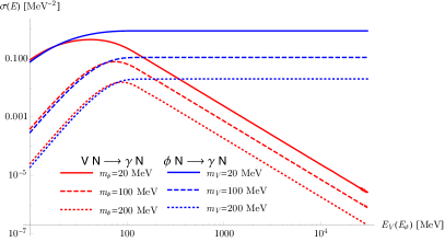
Figure 3: Cross sections for the photoconversion of a massive vector (scalar) mediated by a massive scalar (vector) through the dimension-5 vertex $\mathcal{O}^{s}_{5}$. We fix the mass of the incoming boson to 1 MeV in each case. The cross sections in the case of $\mathcal{O}^{p}_{5}$ are similar, varying only up to a constant factor.

Finally, let us discuss the last possibility which arises from the effective dimension-5 coupling of a massive vector to the pion anomalous decay; $\mathcal{L}\supset\pi^{0}F_{\mu\nu}\tilde{H}^{\mu\nu}$. Again, this permits $VN\to\gamma N$ via the pion-nucleon interaction $ig_{\pi NN}\pi^{0}\bar{\psi}\gamma^{5}\psi$ where the $\pi NN$ coupling is estimated around $g_{\pi NN}\simeq 13$ de Swart et al. (1997). Given that the neutral pion coupling $g_{\pi NN}\bar{N}\gamma^{5}\tau_{3}N\pi^{0}$ is opposite in sign for the proton and neutron, which have opposing isospin charges, $VN\to\gamma N$ scattering via coherent $\pi^{0}$ exchange is suppressed for most isotopes ($\propto(A-2Z)^{2}$). Instead, we consider single-nucleon scattering such that the process is incoherent and proportional to $AF_{p}^{2}(t)$, where $F_{p}(t)$ is the proton form factor, and we take $M=m_{p},m_{n}$.

IV Analysis of the MiniBooNE Data and Constraints

IV.1 MiniBooNE Target-mode and Beam-dump-mode Data

We simulate the LLP flux and event spectra in the MiniBooNE detector by first modeling the flux of charged pions focused by the magnetic horns. This involves a detailed simulation of the Lorentz forces acting on the charged pions and their radiative transport through the horn system, discussed more in Appendix A. Once the charged pion decays are modeled with the decay channels discussed in the previous section, the LLPs produced in these decays are propagated towards the detector and integrated over the its geometrical angular acceptance. This is done for forward and reverse horn currents, corresponding the neutrino and anti-neutrino mode data, respectively Aguilar-Arevalo et al. (2009a, 2018a, 2021a), and separately for the charged and neutral pion decays in the MiniBooNE beam dump without horn focusing Aguilar-Arevalo et al. (2018b). Their subsequent scattering via photonconversion processes $XN\to\gamma N$ give the distribution of $E_{vis}$ (for which we take equal to $E_{\gamma}$ for simplicity, although in principle a smearing matrix should be applied to more diligently model the detector resolution) and $\cos\theta_{\gamma}$ for the reconstructed Cherenkov rings. Given a set of couplings in the decay and scattering models, and the masses of the LLP and the scattering mediator, we then derive fits to the MiniBooNE data.

Example fits to the $\nu$-mode cosine and visible energy spectra are shown in Fig. 4. In the absence of full 2-dimensional data across $(E_{vis},\cos\theta)$ and covariance matrices for both neutrino-mode and anti-neutrino-mode data, we compute a binned $\chi^{2}$ for both the visible energy data and cosine data for $N$ bins;

$$\chi^{2}_{\nu} =\sum_{i=1}^{N}\frac{(d_{i}-s_{i}-b_{i})^{2}}{\sigma_{i}^{2}}.$$ (12)

We then pick the more constraining of the two, either from the cosine or the visible energy data, to set the confidence levels. A similar $\chi^{2}$ is constructed for the anti-neutrino-mode data and the beam-dump-mode data, and we combine all three data sets together in a joint $\chi^{2}$;

$$\chi^{2}_{\textrm{MB}}=\chi^{2}_{\nu}+\chi^{2}_{\overline{\nu}}+\chi^{2}_{\textrm{dump}}$$ (13)

In each model, the signal yield will be schematically proportional to branching ratio in the 3-body decay times scattering cross section, the yield will scale with the coupling product $g^{2}\lambda^{2}y^{2}$. For the operator combinations in model A, we generally fix the mass of the long-lived boson and allow the coupling product and the mass of the mediator in the photoconversion scattering to float in the fit.

It is important to note that the MiniBooNE excess is in time with the Booster Neutrino Beamline 52 MHz beam timing structure Aguilar-Arevalo et al. (2021a), strongly suggesting that the source of the excess is relativistic. This is to be expected from neutrinos or other light particle propagation (studied in this paper) from the target to the detector.

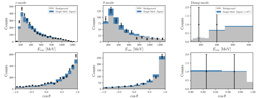
Figure 4: An example fit to the energy and cosine spectra in the MiniBooNE $\nu$-mode (left), $\overline{\nu}$-mode (center), and beam-dump-mode (right) with a long-lived vector $(V)$ produced from the IB2 decay of the charged pions and scattering into a single-photon final state via the SM $\pi^{0}$-nucleon interaction (see Eq. VI). Here the signal in the beam-dump-mode is scaled up by a factor of $10^{5}$ for visualization.

IV.2 MicroBooNE $1\gamma 0p$ Data

The MicroBooNE collaboration performed an analysis of $\Delta\to N\gamma$ resonant production utilizing several final state topologies, namely $1\gamma 0p$ and $1\gamma 1p$ Abratenko et al. (2021). We calculate the expected event rate at MicroBooNE, again employing the simulation procedure for the charged and neutral pions produced in the BNB target and focused through the horn system working in neutrino-mode polarization. This procedure follows exactly as in the previous section for the MiniBooNE analysis, as described in Appendix A, except we now integrate the pion decay products over the solid angle spanned by the MicroBooNE detector’s geometric cross section. In Fig. 5 we show example event spectra produced from 3-body charged meson decays as well as from 2-body $\pi^{0}$ decays using the VIB2 interaction model with couplings to the pion doublet.

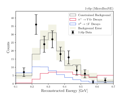
Figure 5: Example event spectra prediction from 2-body decays of $\pi^{0}\to\gamma V$ (blue) and 3-body decays of $\pi^{+}\to\ell\nu V$ (red) at MicroBooNE in the 1$\gamma$0p topology. Here the LLP mass $m_{V}$ is fixed to 5 MeV.

One could also investigate the possibility of using the existing data of higher-energy beam dump experiments like CHARM (400 GeV) or MINER$\nu$A (120 GeV) to constrain the model parameter space. In the case of CHARM, we estimate $\mathcal{O}(10^{17})$ pions produced for $2\cdot 10^{18}$ collected POT Bergsma et al. (1985), and for a detector proximity of 480 meters, the expected flux of LLPs above the 5 GeV energy threshold should be comparatively smaller than those from LSND and KARMEN. Similarly, for MINER$\nu$A, one might examine the $\nu-e$ elastic scattering cross section measurements for events that would mimic the $1\gamma$ final state considered in our phenomenological models Valencia et al. (2019). Although the beam energy at MINER$\nu$A is larger (NuMI beam) than the BNB flux at MicroBooNE, the detector tonnage at the latter is bigger given comparable collected POT and detector baselines. Hence we limit the scope of this analysis to deriving the more stringent constraints from the null results of the MicroBooNE data.

IV.3 Constraints from the LSND and KARMEN Null Results

The parameter space associated with these scenarios get constrained by the LSND data. The LSND experiment used a 800-MeV proton beam. Three analyses, $e^{-}-\nu_{e}$ elastic scattering Auerbach et al. (2001a), charged current reactions of $\nu_{e}$ on ¹²C Auerbach et al. (2001b), and neutrinos from the pion decay in flight Athanassopoulos et al. (1998) can be used to obtain constraints for the parameter space relevant to this solution to the MiniBooNE excess. The data from the elastic and inelastic analyses provide a constraint for the electromagnetic energy in the range 18-35 MeV while the decay-in-flight analysis provides a constraint for the energy range 60-200 MeV.

A summary of the efficiencies and observed counts in each channel is given in Table 1. To determine the constraints set by the null results of each channel on the parameter space of the decay and scattering models we consider, we adopt a single-bin $\chi^{2}$ as a crude test statistic. For example, using the DAR analysis, we look for a contour of constant $\Delta\chi^{2}=s^{2}/1081$, where $s$ is the expected $XN\to\gamma N$ events (multiplied by a flat 37% efficiency) in the energy range $[18,35]$ MeV and 1081 is the number of observed events in the DAR region of interest.

Analysis	$E_{vis}$ Range	$\cos\theta$ Range	Efficiency	Counts
DAR	[$18,35$] MeV	$-1\leq\cos\theta\leq 1$	37%	1081
DIF	[$60,200$] MeV	$\cos\theta<0.8$	10%	50

Table 1: Kinematic regions of interest in the LSND decay-at-rest (DAR) and decay-in-flight (DIF) analyses, their signal efficiencies, and the target number of statistically significant signal counts.

Finally, it may be important to additionally consider inelastic responses of the nucleus in $XN\to\gamma N$ scattering. Although the scope of this work is limited to the null results of LSND, one might also attempt to explain the LSND excess via the inelastic scattering of $XN\to\gamma N^{*},N^{*}\to N\gamma$, which would show up as gamma signal from nuclear de-excitation. We leave this to future work.

Next, we can apply the KARMEN experiment’s observations of the neutral current excitation process ¹²C$(\nu,\nu^{\prime})\to^{12}$C$(1^{+},1;15.1$ MeV$\gamma)$ to place a constraint on photon final states arising from the photoconversion scattering in our phenomenological models Armbruster et al. (1998). This data consists of $4.6\cdot 10^{22}$ collected POT on the tungsten target at the ISIS Reichenbacher (2005); Zeitnitz (1994). The KARMEN detector was situated 17.5m from the target and totaled 56t of liquid scintillating hydrocarbon in a 3.5m$\times$4m$\times$4m geometry. To recast the NC analysis in ref. Armbruster et al. (1998) for our signal model, we will assume the same 12% signal efficiency and 11.5% energy resolution.

V Analysis of the CCM120 Data and CCM200 Projections

In 2019 a six week engineering beam run was performed with the CCM120 detector, named due to it having 120 inward pointing main PMTs. The CCM120 experiment met expectations and performed a sensitive search for sub-GeV dark matter via coherent nuclear scattering with $1.79\times 10^{21}$ Protons On Target (POT) Aguilar-Arevalo et al. (2022a, b). Due to the intense scintillation light production and short 14 cm radiation length in LAr BNL , the relatively large CCM detector has good response to electromagnetic signal events in the energy range from 100 keV up to 100’s of MeV.

Another key feature of CCM is that it uses fast beam and detector timing to isolate prompt ultra-relativistic particles originating in the target. This can distinguish signal from the significantly slower neutron backgrounds that arrive approximately 225 ns after the start of the beam pulse (relativistic particles traverse the 23 m distance in 76.6 ns) Aguilar-Arevalo et al. (2022a). Furthermore, the Lujan beam low duty factor of $\sim 10^{-5}$ and extensive shielding are efficient at rejecting steady state backgrounds from cosmic rays, neutron activation, and internal radioactivity from PMTs and ³⁹Ar.

In order to determine the sensitivity reach of CCM’s ongoing run, we use the beam-on background distribution determined from the recent CCM120 run Aguilar-Arevalo et al. (2022a), with a further expected factor of 100 reduction from extensive improvements in shielding, veto rejection, energy and spatial resolution, particle identification analysis, and reduced beam width. Further details of the signal gamma-ray and electron event reconstruction and background rejection analysis is detailed in the recent CCM120 ALP search Aguilar-Arevalo et al. (2023), which share many similarities.

Since our MiniBooNE excess explanation requires dominant contributions from the charged pion decay (otherwise the data in the beam-dump mode measurement would rule it out), the constraint for this parameter space mostly emerges from the elastic and inelastic analyses. The visible energy distribution for the events at CCM120 is in the range 10-70 MeV (as shown in Fig. 6) for various scenarios described in § II. In Fig. 7, we show the allowed parameter space where the MiniBooNE excess can be explained after satisfying the LSND constraints, in addition to the comparison with projected sensitivities for CCM assuming the null hypothesis.

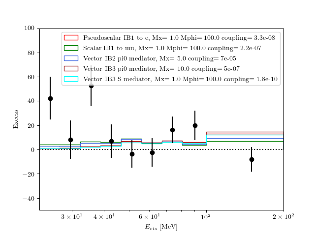
Figure 6: The CCM120 high energy subtraction spectrum used for the search search. Only events between 22.4 and 200 MeV reconstructed energy were included in this spectrum. Also shown are example spectra from the Dark Sector for the 5 models tested with CCM120, using points on the 68% confidence level.

VI Results

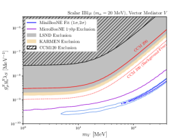
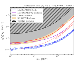
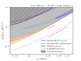
Figure 7: Parameter space for the two-mediator models, consisting of one long-lived boson produced through charged pion three-body decays and scattering via a secondary heavy mediator are shown. Left: a 20 MeV scalar $\phi$ coupling to muons and scattering via a vector mediator $V$ as in Eq. 14. Center: a 0.5 MeV pseudoscalar $a$ coupling to electrons and scattering via a vector mediator $V$ as in Eq. 15. Right: a 20 MeV vector $V$ coupling through the IB3 pion contact interaction and scattering via a massive scalar $\phi$ as in Eq. VI. The exclusions (CCM120, KARMEN, LSND, and MicroBooNE) and projections for CCM200 are shown at 95% C.L., while the MiniBooNE fits are shown at 68% and 95% C.L. in dark and light blue, respectively.

In Fig. 7 we show the resulting constraints set by the CCM120 data, projections for CCM200 along with the preferred MiniBooNE regions (CLs at 1$\sigma$ and 2$\sigma$), and the constraints from the LSND DIF and DAR analyses (see Table 1) for three possible decay models and scattering model scenarios. These models are named according to (i) the type of long-lived boson and decay mode (see Fig. 1), e.g. Scalar IB1$\mu$ to indicate the IB1 decay channel through a coupling to the muon leg, and (ii) the type of mediator (scalar, pseudoscalar, or vector) used in the scattering via the interactions in Fig. 2. All curves correspond to 95% C.L. Also shown are the limits extracted from the MicroBooNE $1{\gamma}0p$ data.

Beginning with Fig. 7 (left), we consider the parameter space for a long-lived scalar particle $\phi$ produced via the IB1 decay $\pi^{\pm}\to\mu\nu\phi$ through a muonic coupling, and scattering through $\phi N\to\gamma N$ photoconversion via a massive vector mediator $V$. The decay and scattering are described by the phenomenological Lagrangian

$$\mathcal{L}_{int}\supset g_{\mu}^{S}\phi\bar{\mu}\mu+y_{n}^{V}V_{\mu}\bar{N}\gamma^{\mu}N-\frac{\lambda_{S}}{4}\phi F_{\mu\nu}H^{\mu\nu}\,+\textrm{h.c.}$$ (14)

with $H_{\mu\nu}\equiv\partial_{\mu}V_{\nu}-\partial_{\nu}V_{\mu}$ and vector mass $m_{V}>m_{\phi}$. The event rate is proportional to the coupling product $g_{\mu}^{S}y_{n}^{V}\lambda_{S}$. For this setup, we can fix the mass of the long-lived scalar to 20 MeV and vary $m_{V}$, for which we find that the fit to the MiniBooNE target and dump mode data lies around the scale $g_{\mu}^{S}y_{n}^{V}\lambda_{S}\simeq 10^{-9}$ MeV^-1 at the 1$\sigma$ and 2$\sigma$ levels. The black hatched region is constrained by the CCM120 data, while constraints by LSND shown in olive are more stringent but do not rule out any of the preferred parameter space from the MiniBooNE fit – conversely, MicroBooNE’s $1\gamma 0p$ data excludes more parameter space up to about a factor of 2 larger in the coupling product across all mediator masses, and one could expect that future SBN experiments with larger detector exposure could test the MiniBooNE preferred region completely.

In Fig. 7 (center), the parameter space for a long-lived pseudoscalar coupling to electrons and produced through IB1 $\pi^{\pm}\to e\nu a$ decays is shown as a function of the coupling product and mass of a vector mediator taking place in the $aN\to\gamma N$ scattering via similar interactions,

$$\mathcal{L}_{int}\supset-ig_{e}^{P}a\bar{\mu}\gamma^{5}\mu+y_{n}^{V}V_{\mu}\bar{N}\gamma^{\mu}N-\frac{\lambda_{P}}{4}aF_{\mu\nu}\tilde{H}^{\mu\nu}\,+\textrm{h.c.}$$ (15)

We fix the pseudoscalar mass $m_{a}<2m_{e}\simeq 1$ MeV, otherwise $a\to e^{+}e^{-}$ decays would be kinematically allowed and may be incompatible with the excess signal, and again take $m_{V}>m_{a}$. In this scenario the event rate is proportional to the coupling product $g_{e}^{P}y_{n}^{V}\lambda_{P}$, and a result similar to Fig. 7, left is found where the entirety of the MiniBooNE preferred region is allowed by the existing constraints we have considered.

In Fig. 7 (right) we consider a third scenario in which a massive vector mediator is long-lived and couples to the charged pion through a contact interactions, and subsequently scatters via a massive scalar mediator with mass $m_{\phi}>m_{V}$. We take the effective interaction Lagrangian

$$\mathcal{L}_{int}\supset \,y_{n}^{S}\phi\overline{N}N-\frac{\lambda_{S}}{4}aF_{\mu\nu}\tilde{H}^{\mu\nu}$$

$$-ig_{\pi}^{V}\pi^{+}\bar{\mu}\gamma^{\rho}(1-\gamma^{5})\nu V_{\rho}\,+\,\textrm{h.c.}$$ (16)

In the second class of phenomenological model, we consider a single long-lived vector mediator that couples to quarks and enters the pion sector via the $\chi$-PT Lagrangian in Eq. VI;

$$\mathcal{L}_{int}\supset \,ig_{\pi^{\pm}}V_{\mu}\pi^{+}(\partial^{\mu}\pi^{-})+g_{\pi^{0}}\frac{e}{16\pi f_{\pi}}\pi^{0}F_{\mu\nu}\tilde{H}^{\mu\nu}$$

$$-ig_{\pi NN}\pi^{0}\overline{N}\gamma^{5}\tau_{3}N$$ (17)

In Fig. 8 we show the parameter space sensitivities and constraints for the IB2 decay model for $m_{V}=5,10,20$ MeV. The CLs for the MiniBooNE fit are shown (blue) for the combination of $\nu$, $\bar{\nu}$, and beam-dump-mode runs, exclusions set by the CCM120 engineering run are shown by the black hatched region, and future sensitivity expected in CCM200 with upgrades (red). Also shown are constraints from LSND (olive) and pion decay width measurements (gray). In this case we have production channels from both charged pion decays ($\pi^{\pm}\to\ell\nu V$), for which we take the IB2 decay mode as a benchmark, and neutral pion decays ($\pi^{0}\to V\gamma$). Constraints from $\pi^{\pm}$ decay width measurements can be directly applied to this parameter space in terms of $g_{\pi^{\pm}}$, and for these we take the bounds from PIENU Aguilar-Arevalo et al. (2021b) which have set constraints on invisible radiative decays $\pi^{\pm}\to e^{\pm}\nu X$ and $\pi^{\pm}\to\mu\nu^{\pm}X$ dependent on the $X$ mass.

As the vector mass transitions from 5 to 20 MeV, the preferred solution transitions from one in which the signal is dominated by the charged pion decay channel to one where both charged and neutral meson decays are contributing to the signal in MiniBooNE equally. In this limiting case at $m_{V}=20$ MeV, the couplings $g_{\pi^{\pm}}\simeq g_{\pi^{0}}$, but the $\chi^{2}_{min}$ is strongly excluded by the LSND and the CCM120 engineering run observations as shown in the bottom panels of Fig. 8. In addition, constraints from $\pi^{0}$ decay width measurements apply to the $g_{\pi^{0}}$ coupling in this parameter space.

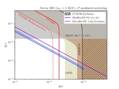
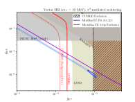
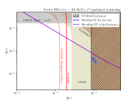
Figure 8: Parameter space for the single mediator scenario where a massive vector $V$ couples to the pion doublet via charged pion coupling $g_{\pi^{\pm}}$ and neutral pion coupling $g_{\pi^{0}}$ as in Eq. VI. We vary the vector mass $m_{V}$ from left to right as $5$ MeV (top), $10$ MeV (lower left), and $20$ MeV (lower right).The exclusions (CCM120, KARMEN, LSND, and MicroBooNE) and projections for CCM200 are shown at 95% C.L., while the MiniBooNE fits are shown at 68% and 95% C.L. in dark and light blue, respectively.

VII Conclusions

The rare three-body decays of charged pions and kaons to new states in the MeV mass scale as a dark-sector explanation for the MiniBooNE excess has shed light on a potential correlation between the mesonic sector and new physics solutions. By investigating an extended range of phenomenological models, we have demonstrated that these scenarios, incorporating long-lived particles generated in the three-body decays of charged mesons and two-body anomalous decays of neutral mesons, can be consistent with constraints from LSND, KARMEN, and MicroBooNE experiments. In particular, we found that in the context of these models with a long-lived particle and a heavy mediator to facilitate photoconversion scattering, the MiniBooNE excess data preferred a mediator in the mass range $m_{Y}\gtrsim 10-100$ MeV. In all cases, scattering with detector atomic nucleii was considered, so it may be interesting to probe new mediators in this mass range with generalized hadronic couplings in separate experiments. Secondly, the inelastic nuclear responses to the mediators we have considered is an interesting possibility to study, namely in the context of the LSND excess which we have set aside for the time being. One could also examine the same inelastic channels as they contribute to the event spectra at KARMEN, MiniBooNE, MicroBooNE, and CCM, although this requires a detailed shell-model description of the nucleus coupled to the new mediators we have used.

The forthcoming analysis of the current CCM200 data taking campaign will have the ability to test dark-sector explanations to the MiniBooNE excess, especially for new long-lived particles coupled to the pion doublet; as a stopped-pion experiment, it can leverage the neutral pion production and its close proximity to the proton beam target. In this way, stopped-pion experiments have more sensitivity via the neutral pion channels to probe this set of solutions in a complementary way to short baseline experiments, whose magnetic horns produce instead a focused flux of charged mesons. Long-lived vector mediators that couple to the pion doublet around 5 MeV in mass, as preferred by the fits to MiniBooNE data, are now susceptible to searches through both stopped-pion experiments as well as rare meson decay searches. Though not within the scope of this work, there is no reason to not expand the dark sector couplings to the meson octet which would include kaons, or to the broader hadronic spectrum of baryons and vector mesons. This analysis motivates such cases through the advantage of correlated couplings which open up multiple production and detection channels to constrain, and hopefully discover, solutions to anomalies in this fashion.

Appendix A Meson Flux Simulations at the BNB

To simulate the focused charged meson decays that take place in the BNB horn system, we begin by simulating the proton beam spot that sources the charged mesons, shown in Fig. 9, based on the normal distribution of protons given in Schmitz (2008) which source a $\pi^{\pm}$ at beam spot position $(x,y)$ and depth $z$ into the target given from the interaction probability $1-e^{-\sigma(p)nz}$ based on the pion production cross section in Eq. 19 and Be density $n=1.85$ g/cm³. The proton momenta are also generated by a parameterization.

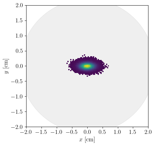
Figure 9: Simulation of the BNB beam spot distribution of protons on target as a function of $(x,y)$ over the face of the Be target, shown in gray.

We use this beam spot to generate a monte carlo sample of pion production vertices. Their momenta and production angles with respect to the progenitor proton direction can be expressed using the Sanford-Wang parameterization given in ref. Aguilar-Arevalo et al. (2009b), shown in Fig. 10. This scheme parameterizes the total pion production cross section as follows;

$$\dfrac{\partial^{2}\sigma(p+\textrm{Be}\to\pi^{\pm}+X)}{\partial p\partial\Omega}=c_{1}p^{c_{2}}\bigg{(}1-\frac{p}{p_{B}-c_{9}}\bigg{)}\exp\bigg{(}-c_{3}\frac{p^{c_{4}}}{p_{B}^{c_{5}}}-c_{6}\theta(p-c_{7}p_{B}(\cos\theta)^{c_{8}}\bigg{)}$$ (18)

where the constants associated with $\pi^{+}$ ($\pi^{-}$) production are repeated in Table 2 for convenience.

Type	$c_{1}$	$c_{2}$	$c_{3}$	$c_{4}$	$c_{5}$	$c_{6}$	$c_{7}$	$c_{8}$	$c_{9}$
$\pi^{+}$	220.7	1.080	1.0	1.978	1.32	5.572	0.0868	9.686	1.0
$\pi^{-}$	213.7	0.9379	5.454	1.210	1.284	4.781	0.07338	8.329	1.0

Table 2: Sanford-Wang cross section parameters at the BNB target.

while the total cross section is parameterized as

$$\sigma(p)=a+bp^{n}+c(\ln(p))^{2}+d\ln(p)$$ (19)

with

$$a =307.8$$

$$b =0.897$$

$$c =-2.598$$

$$d =-4.973$$

$$n =0.003$$ (20)

Taking the position $(x,y,z)$ from the beam spot simulation and the momentum, polar angle, and azimuthal angle $(p,\cos\theta,\phi)$ from a weighted MC simulation of the Sanford-Wang cross section, the pion flux is prepared for simulated transport through the remainder of the beam target and horn system. For this we use a simple geometric model of the BNB horn shape and magnetic field profile as inputs to a Runge-Kutta charged particle transport routine. Some sample trajectories are shown in Fig. 11.

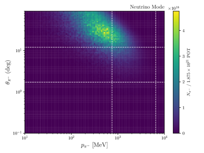
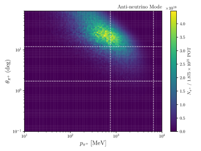
Figure 10: Charged pion fluxes produced at the BNB via a monte carlo treatment of the Sanford-Wang parameterization of the charged pion production cross section.

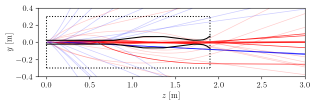
Figure 11: Simulation of the BNB horn with example trajectories showing the $\pi^{+}$ (red) and $\pi^{-}$ (blue) transport in the horn system for FHC polarization.

The post-horn flux distribution using $5\cdot 10^{5}$ simulated POT is shown in Fig. 12 as a function of pion angle with respect to the beam axis. For comparison, the equivalent detector solid angle coverages of MicroBooNE and MiniBooNE are 1.2 mrad and 3 mrad, respectively. We validate this distribution in a pragmatic way by checking that it predicts a neutrino spectrum at the MiniBooNE detector that is consistent with what is reported by the collaboration. To do this, we take the focused $\pi^{\pm}$ fluxes predicted by Sanford-Wang and perform a 2-body decay monte carlo algorithm on the charged pions, allowing them to decay to $\nu_{\mu}$, $\mu$ at some distance $x$ away from the production site in the target, where $x$ itself is drawn from a distribution like $\exp(-x/v\tau_{\pi^{\pm}})$ using the pion lifetimes.

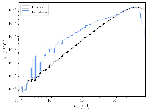
Figure 12: The pre-horn $\pi^{+}$ flux (black) using the Sanford-Wang parameterized cross section convolved with the BNB proton beamspot, and the post-horn flux (blue) after modeling the transport through the magnetic horn system are both shown as a function of the pion angle with respect to the beam axis. In both cases $5\cdot 10^{5}$ simulated POT were used.

Additionally, the distributions for neutral $\pi^{0}$ that are produced in the BNB target and the dump are shown in Fig. 13. The differences in the $\pi^{0}$ energy and angle distributions at the target versus the dump can be attributed to the larger size of the dump and the differences in material on which the beam impinges. To simulate events from the 2-body decays of $\pi^{0}\to\gamma X$, we perform the decay simulation in the pion rest frame and boost $X$ into the lab frame. Since $X$ is long-lived and weakly coupled, it can be invisibly transported to the detector, where we must check that the $X$ production angle with respect to the beam line is small enough to be captured within the detector solid angle. To give a sense of the angular coverage, we show the effective cutoff anlge by the green lines in Fig. 13.

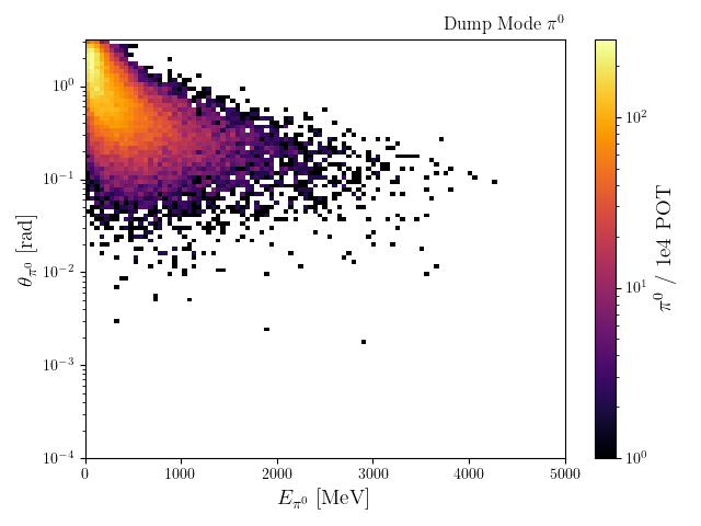
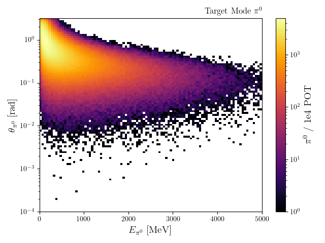
Figure 13: Beam-dump-mode and target-mode $\pi^{0}$ fluxes, generated from GEANT4 simulation, at MiniBooNE as a function of their kinetic energy and angle of travel with respect to the beam axis. The green lines indicate roughly where the cutoff lies for decay products lying within the solid angle of the detector.

Appendix B Treatment of 3-body Decay Kinematics

For the charged meson three-body decay $M(P)\to\ell(p_{1})\nu(p_{2})a(p_{3})$, we make use of the Dalitz variables $m_{ij}^{2}=(p_{i}+p_{j})^{2}$. In the lab frame, we have

$$m_{12}^{2} =(p_{1}+p_{2})^{2}=(P-p_{3})^{2}=M^{2}-2ME_{a}+m_{a}^{2}$$ (21)

$$m_{23}^{2} =(p_{2}+p_{3})^{2}=(P-p_{1})^{2}=M^{2}-2ME_{\ell}+m_{\ell}^{2}$$ (22)

$$m_{13}^{2} =(p_{1}+p_{3})^{2}=(P-p_{2})^{2}=M^{2}-2ME_{\nu}$$ (23)

$$m_{13}^{2} =M^{2}+m_{\ell}^{2}+m_{a}^{2}-m_{12}^{2}-m_{23}^{2}.$$ (24)

This set of variables allows us to write

$$d\Gamma=\dfrac{1}{(2\pi)^{3}32M^{3}}\braket{}{M}{{}^{2}}dm_{23}^{2}dm_{12}^{2}$$ (25)

and re-express $m_{12}^{2}$ in terms of $E_{a}$, since $|dm_{12}^{2}|=2MdE_{a}$, allowing us to integrate over $m_{23}^{2}$;

$$\dfrac{d\Gamma}{dE_{a}}=\int^{(m_{23}^{2})_{max}}_{(m_{23}^{2})_{min}}\dfrac{1}{(2\pi)^{3}16M^{2}}\braket{}{M}{{}^{2}}dm_{23}^{2}.$$ (26)

This has bounds

$$(m_{23}^{2})^{max}_{min}=(E_{2}^{*}+E_{3}^{*})^{2}-\bigg{(}E_{2}^{*}\mp\sqrt{{E_{3}^{*}}^{2}-m_{a}^{2}}\,\bigg{)}$$ (27)

with the starred energies defined as

$$E_{2}^{*} =\dfrac{m_{12}^{2}-m_{\ell}^{2}}{2m_{12}}$$ (28)

$$E_{3}^{*} =\dfrac{M^{2}-m_{12}^{2}-m_{a}^{2}}{2m_{12}}$$ (29)

Finally, we can integrate over $E_{a}$ making use of the fact that $m_{\ell}^{2}<m_{12}^{2}<M^{2}+m_{a}^{2}-2Mm_{a}$ to get the $E_{a}$ limits;

$$m_{a}<E_{a}<\dfrac{M^{2}+m_{a}^{2}-m_{\ell}^{2}}{2M}.$$ (30)

Using this integration scheme, we show the total branching ratios for IB1, IB2, and IB3/contact decays, broken down by decay channel ($\ell=e$ or $\ell=\mu$), in Fig. 14.

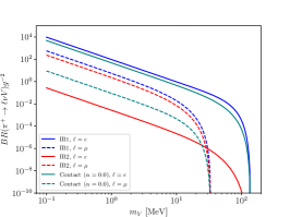
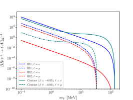
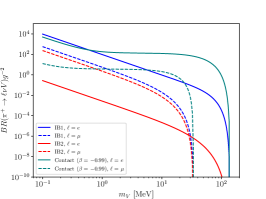
Figure 14: Branching Ratios for Vector IB2 and IB3 interactions with various choices of the Ward parameter $r$ defined by Eq. LABEL:eq:ward.

Appendix C $\chi$PT

$$\mathcal{L}_{hp}^{\chi PT} \supset\frac{f_{\pi}^{2}}{4}\textrm{Tr}\bigg{[}(\partial_{\mu}\mathbf{U}-iV_{\mu}\{\mathbf{g}_{X},\mathbf{U}\})(\partial^{\mu}\mathbf{U}+iV^{\mu}\{\mathbf{g}_{X},\mathbf{U}\})\bigg{]}$$ (31)

where the octet of meson states are contained in the Goldstone field $\Phi$ in the 3-flavor quark basis,

$$\mathbf{U}=e^{i\sqrt{2}\Phi/f_{\pi}},\,\,\Phi=\begin{pmatrix}\frac{\pi^{0}}{\sqrt{2}}+\frac{\eta_{8}}{\sqrt{6}}&\pi^{+}&K^{+}\\ \pi^{-}&-\frac{\pi^{0}}{\sqrt{2}}+\frac{\eta_{8}}{\sqrt{6}}&K^{0}\\ K^{-}&\overline{K}^{0}&-\frac{2\eta_{8}}{\sqrt{6}}\end{pmatrix}.$$ (32)

Further, for simplicity we select only up- and down-type quark couplings in the coupling matrix $\mathbf{g}_{X}$;

$$\mathbf{g}_{X}\equiv\begin{pmatrix}g_{u}&0&0\\ 0&g_{d}&0\\ 0&0&0\end{pmatrix}$$ (33)

After expanding out Eq. 31, our effective Lagrangian below the QCD scale will contain the operator

$$\mathcal{L}_{hp}^{\chi PT}\supset i(g_{u}-g_{d})V_{\mu}\pi^{+}(\partial^{\mu}\pi^{-})$$ (34)

If instead coupling a vector to the meson sector, we could also introduce a SM-singlet scalar $\phi$ into the $\chi$PT potential, we may have terms such as

$$V(\phi,\mathbf{U})\supset(\phi^{\dagger}+\phi)\textrm{Tr}\big{[}\mathbf{U}^{\dagger}\mathbf{g_{\phi}}\mathbf{U}\big{]}$$ (35)

which leads to cubic interactions like $\phi\pi^{+}\pi^{-}$ after expanding out the trace. We leave this possibility to a future work.

References

- Aguilar-Arevalo et al. (2009a) A. A. Aguilar-Arevalo et al. (MiniBooNE), Phys. Rev. Lett. 102, 101802 (2009a), arXiv:0812.2243 [hep-ex] .
- Aguilar-Arevalo et al. (2018a) A. A. Aguilar-Arevalo et al. (MiniBooNE), Phys. Rev. Lett. 121, 221801 (2018a), arXiv:1805.12028 [hep-ex] .
- Aguilar-Arevalo et al. (2021a) A. A. Aguilar-Arevalo et al. (MiniBooNE), Phys. Rev. D 103, 052002 (2021a), arXiv:2006.16883 [hep-ex] .
- Aguilar-Arevalo et al. (2018b) A. A. Aguilar-Arevalo et al. (MiniBooNE DM), Phys. Rev. D 98, 112004 (2018b), arXiv:1807.06137 [hep-ex] .
- Sorel et al. (2004) M. Sorel, J. M. Conrad, and M. Shaevitz, Phys. Rev. D 70, 073004 (2004), arXiv:hep-ph/0305255 .
- Karagiorgi et al. (2009) G. Karagiorgi, Z. Djurcic, J. M. Conrad, M. H. Shaevitz, and M. Sorel, Phys. Rev. D 80, 073001 (2009), [Erratum: Phys.Rev.D 81, 039902 (2010)], arXiv:0906.1997 [hep-ph] .
- Collin et al. (2016) G. H. Collin, C. A. Argüelles, J. M. Conrad, and M. H. Shaevitz, Phys. Rev. Lett. 117, 221801 (2016), arXiv:1607.00011 [hep-ph] .
- Giunti and Laveder (2011a) C. Giunti and M. Laveder, Phys. Rev. D 84, 073008 (2011a), arXiv:1107.1452 [hep-ph] .
- Giunti and Laveder (2011b) C. Giunti and M. Laveder, Phys. Lett. B 706, 200 (2011b), arXiv:1111.1069 [hep-ph] .
- Gariazzo et al. (2017) S. Gariazzo, C. Giunti, M. Laveder, and Y. F. Li, JHEP 06, 135 (2017), arXiv:1703.00860 [hep-ph] .
- Böser et al. (2020) S. Böser, C. Buck, C. Giunti, J. Lesgourgues, L. Ludhova, S. Mertens, A. Schukraft, and M. Wurm, Prog. Part. Nucl. Phys. 111, 103736 (2020), arXiv:1906.01739 [hep-ex] .
- Kopp et al. (2011) J. Kopp, M. Maltoni, and T. Schwetz, Phys. Rev. Lett. 107, 091801 (2011), arXiv:1103.4570 [hep-ph] .
- Kopp et al. (2013) J. Kopp, P. A. N. Machado, M. Maltoni, and T. Schwetz, JHEP 05, 050 (2013), arXiv:1303.3011 [hep-ph] .
- Dentler et al. (2018) M. Dentler, A. Hernández-Cabezudo, J. Kopp, P. A. N. Machado, M. Maltoni, I. Martinez-Soler, and T. Schwetz, JHEP 08, 010 (2018), arXiv:1803.10661 [hep-ph] .
- Abazajian et al. (2012) K. N. Abazajian et al., (2012), arXiv:1204.5379 [hep-ph] .
- Conrad et al. (2013) J. M. Conrad, C. M. Ignarra, G. Karagiorgi, M. H. Shaevitz, and J. Spitz, Adv. High Energy Phys. 2013, 163897 (2013), arXiv:1207.4765 [hep-ex] .
- Diaz et al. (2020) A. Diaz, C. A. Argüelles, G. H. Collin, J. M. Conrad, and M. H. Shaevitz, Phys. Rept. 884, 1 (2020), arXiv:1906.00045 [hep-ex] .
- Asaadi et al. (2018) J. Asaadi, E. Church, R. Guenette, B. J. P. Jones, and A. M. Szelc, Phys. Rev. D 97, 075021 (2018), arXiv:1712.08019 [hep-ph] .
- Karagiorgi et al. (2012) G. Karagiorgi, M. H. Shaevitz, and J. M. Conrad, (2012), arXiv:1202.1024 [hep-ph] .
- Pas et al. (2005) H. Pas, S. Pakvasa, and T. J. Weiler, Phys. Rev. D 72, 095017 (2005), arXiv:hep-ph/0504096 .
- Döring et al. (2020) D. Döring, H. Päs, P. Sicking, and T. J. Weiler, Eur. Phys. J. C 80, 1202 (2020), arXiv:1808.07460 [hep-ph] .
- Kostelecky and Mewes (2004) V. A. Kostelecky and M. Mewes, Phys. Rev. D 69, 016005 (2004), arXiv:hep-ph/0309025 .
- Katori et al. (2006) T. Katori, V. A. Kostelecky, and R. Tayloe, Phys. Rev. D 74, 105009 (2006), arXiv:hep-ph/0606154 .
- Diaz and Kostelecky (2011) J. S. Diaz and V. A. Kostelecky, Phys. Lett. B 700, 25 (2011), arXiv:1012.5985 [hep-ph] .
- Diaz and Kostelecky (2012) J. S. Diaz and A. Kostelecky, Phys. Rev. D 85, 016013 (2012), arXiv:1108.1799 [hep-ph] .
- Gninenko (2009) S. N. Gninenko, Phys. Rev. Lett. 103, 241802 (2009), arXiv:0902.3802 [hep-ph] .
- Gninenko and Gorbunov (2010) S. N. Gninenko and D. S. Gorbunov, Phys. Rev. D 81, 075013 (2010), arXiv:0907.4666 [hep-ph] .
- Bai et al. (2016) Y. Bai, R. Lu, S. Lu, J. Salvado, and B. A. Stefanek, Phys. Rev. D 93, 073004 (2016), arXiv:1512.05357 [hep-ph] .
- Moss et al. (2018) Z. Moss, M. H. Moulai, C. A. Argüelles, and J. M. Conrad, Phys. Rev. D 97, 055017 (2018), arXiv:1711.05921 [hep-ph] .
- Bertuzzo et al. (2018) E. Bertuzzo, S. Jana, P. A. N. Machado, and R. Zukanovich Funchal, Phys. Rev. Lett. 121, 241801 (2018), arXiv:1807.09877 [hep-ph] .
- Ballett et al. (2019) P. Ballett, S. Pascoli, and M. Ross-Lonergan, Phys. Rev. D 99, 071701 (2019), arXiv:1808.02915 [hep-ph] .
- Fischer et al. (2020) O. Fischer, A. Hernández-Cabezudo, and T. Schwetz, Phys. Rev. D 101, 075045 (2020), arXiv:1909.09561 [hep-ph] .
- Moulai et al. (2020) M. H. Moulai, C. A. Argüelles, G. H. Collin, J. M. Conrad, A. Diaz, and M. H. Shaevitz, Phys. Rev. D 101, 055020 (2020), arXiv:1910.13456 [hep-ph] .
- Dentler et al. (2020) M. Dentler, I. Esteban, J. Kopp, and P. Machado, Phys. Rev. D 101, 115013 (2020), arXiv:1911.01427 [hep-ph] .
- de Gouvêa et al. (2020) A. de Gouvêa, O. L. G. Peres, S. Prakash, and G. V. Stenico, JHEP 07, 141 (2020), arXiv:1911.01447 [hep-ph] .
- Datta et al. (2020) A. Datta, S. Kamali, and D. Marfatia, Phys. Lett. B 807, 135579 (2020), arXiv:2005.08920 [hep-ph] .
- Dutta et al. (2020) B. Dutta, S. Ghosh, and T. Li, Phys. Rev. D 102, 055017 (2020), arXiv:2006.01319 [hep-ph] .
- Abdallah et al. (2020) W. Abdallah, R. Gandhi, and S. Roy, JHEP 12, 188 (2020), arXiv:2006.01948 [hep-ph] .
- Abdullahi et al. (2021) A. Abdullahi, M. Hostert, and S. Pascoli, Phys. Lett. B 820, 136531 (2021), arXiv:2007.11813 [hep-ph] .
- Liao and Marfatia (2016) J. Liao and D. Marfatia, Phys. Rev. Lett. 117, 071802 (2016), arXiv:1602.08766 [hep-ph] .
- Carena et al. (2017) M. Carena, Y.-Y. Li, C. S. Machado, P. A. N. Machado, and C. E. M. Wagner, Phys. Rev. D 96, 095014 (2017), arXiv:1708.09548 [hep-ph] .
- Abdallah et al. (2021) W. Abdallah, R. Gandhi, and S. Roy, Phys. Rev. D 104, 055028 (2021), arXiv:2010.06159 [hep-ph] .
- Jordan et al. (2019) J. R. Jordan, Y. Kahn, G. Krnjaic, M. Moschella, and J. Spitz, Phys. Rev. Lett. 122, 081801 (2019), arXiv:1810.07185 [hep-ph] .
- Dutta et al. (2021) B. Dutta, D. Kim, A. Thompson, R. T. Thornton, and R. G. Van de Water, (2021), arXiv:2110.11944 [hep-ph] .
- Barger et al. (2012) V. Barger, C.-W. Chiang, W.-Y. Keung, and D. Marfatia, Phys. Rev. Lett. 108, 081802 (2012), arXiv:1109.6652 [hep-ph] .
- Carlson and Rislow (2012) C. E. Carlson and B. C. Rislow, Phys. Rev. D 86, 035013 (2012), arXiv:1206.3587 [hep-ph] .
- Laha et al. (2014) R. Laha, B. Dasgupta, and J. F. Beacom, Phys. Rev. D 89, 093025 (2014), arXiv:1304.3460 [hep-ph] .
- Bakhti and Farzan (2017) P. Bakhti and Y. Farzan, Phys. Rev. D 95, 095008 (2017), arXiv:1702.04187 [hep-ph] .
- Altmannshofer et al. (2020) W. Altmannshofer, S. Gori, and D. J. Robinson, Phys. Rev. D 101, 075002 (2020), arXiv:1909.00005 [hep-ph] .
- Krnjaic et al. (2020) G. Krnjaic, G. Marques-Tavares, D. Redigolo, and K. Tobioka, Phys. Rev. Lett. 124, 041802 (2020), arXiv:1902.07715 [hep-ph] .
- Aguilar-Arevalo et al. (2023) A. A. Aguilar-Arevalo et al. (CCM), Phys. Rev. D 107, 095036 (2023), arXiv:2112.09979 [hep-ph] .
- Dutta et al. (2022) B. Dutta, S. Ghosh, and J. Kumar, in Snowmass 2021 (2022) arXiv:2203.07786 [hep-ph] .
- Kaneta et al. (2017) K. Kaneta, H.-S. Lee, and S. Yun, Phys. Rev. Lett. 118, 101802 (2017), arXiv:1611.01466 [hep-ph] .
- Berger et al. (2020) D. Berger, A. Rajaraman, and J. Kumar, Pramana 94, 133 (2020), arXiv:1903.10632 [hep-ph] .
- de Swart et al. (1997) J. J. de Swart, M. C. M. Rentmeester, and R. G. E. Timmermans, PiN Newslett. 13, 96 (1997), arXiv:nucl-th/9802084 .
- Donoghue and Holstein (1989) J. F. Donoghue and B. R. Holstein, Phys. Rev. D 40, 2378 (1989).
- Bryman et al. (1982) D. Bryman, P. Depommier, and C. Leroy, Physics Reports 88, 151 (1982).
- Khodjamirian and Wyler (2001) A. Khodjamirian and D. Wyler, (2001), 10.1142/9789812777478_0014, arXiv:hep-ph/0111249 .
- Beneke et al. (2018) M. Beneke, V. M. Braun, Y. Ji, and Y.-B. Wei, JHEP 07, 154 (2018), arXiv:1804.04962 [hep-ph] .
- Beneke and Rohrwild (2011) M. Beneke and J. Rohrwild, Eur. Phys. J. C 71, 1818 (2011), arXiv:1110.3228 [hep-ph] .
- Bansal and Mahajan (2021) A. Bansal and N. Mahajan, Phys. Rev. D 103, 056017 (2021), arXiv:2010.00549 [hep-ph] .
- Abratenko et al. (2021) P. Abratenko et al. (MicroBooNE), (2021), arXiv:2110.00409 [hep-ex] .
- Bergsma et al. (1985) F. Bergsma et al., Physics Letters B 157, 458 (1985).
- Valencia et al. (2019) E. Valencia et al. (MINERvA), Phys. Rev. D 100, 092001 (2019), arXiv:1906.00111 [hep-ex] .
- Auerbach et al. (2001a) L. B. Auerbach et al. (LSND), Phys. Rev. D 63, 112001 (2001a), arXiv:hep-ex/0101039 .
- Auerbach et al. (2001b) L. B. Auerbach et al. (LSND), Phys. Rev. C 64, 065501 (2001b), arXiv:hep-ex/0105068 .
- Athanassopoulos et al. (1998) C. Athanassopoulos et al. (LSND), Phys. Rev. C 58, 2489 (1998), arXiv:nucl-ex/9706006 .
- Armbruster et al. (1998) B. Armbruster et al., Physics Letters B 423, 15 (1998).
- Reichenbacher (2005) J. Reichenbacher, Final KARMEN results on neutrino oscillations and neutrino nucleus interactions in the energy regime of supernovae, Other thesis (2005).
- Zeitnitz (1994) B. Zeitnitz (KARMEN), Prog. Part. Nucl. Phys. 32, 351 (1994).
- Aguilar-Arevalo et al. (2022a) A. A. Aguilar-Arevalo et al. (CCM), Phys. Rev. D 106, 012001 (2022a), arXiv:2105.14020 [hep-ex] .
- Aguilar-Arevalo et al. (2022b) A. A. Aguilar-Arevalo et al. (CCM), Phys. Rev. Lett. 129, 021801 (2022b), arXiv:2109.14146 [hep-ex] .
- (73) BNL, “Liquid argon properties, https://lar.bnl.gov/properties/,” .
- Aguilar-Arevalo et al. (2021b) A. Aguilar-Arevalo et al. (PIENU), Phys. Rev. D 103, 052006 (2021b), arXiv:2101.07381 [hep-ex] .
- Schmitz (2008) D. W. Schmitz, A Measurement of Hadron Production Cross Sections for the Simulation of Accelerator Neutrino Beams and a Search for to Sscillations in the about equals Region, Ph.D. thesis, Columbia U. (2008).
- Aguilar-Arevalo et al. (2009b) A. A. Aguilar-Arevalo et al. (MiniBooNE), Phys. Rev. D 79, 072002 (2009b), arXiv:0806.1449 [hep-ex] .