Finding and improving bounds of real functions by thermodynamic arguments

Abstract

The possibility of stating the second law of thermodynamics in terms of the increasing behaviour of a physical property establishes a connection between that branch of physics and the theory of algebraic inequalities. We use this connection to show how some well-known inequalities such as the standard bounds for the logarithmic function or generalizations of Bernoulli’s inequality can be derived by thermodynamic methods. Additionally, we show that by comparing the global entropy production in processes implemented with decreasing levels of irreversibility but subject to the same change of state of one particular system, we can find progressively better bounds for the real function that represents the entropy variation of the system. As an application, some new families of bounds for the function $\log(1+x)$ are obtained by this method.

I Introduction

In addition to the interest that algebraic inequalities present from a purely mathematical point of view, they are also fundamental tools in physics, economics, statistics and likely in any branch of science that employs mathematics in its formal description. Inequalities involving elementary functions appear so frequently in other disciplines that the problem of bounding them is an important issue. One of the most ubiquitous elementary functions is the (natural) logarithm, for which the following bounds are probably well-known by the reader:

$$\dfrac{x}{1+x}\leq\log(1+x)\leq x,\hskip 5.69046ptx>-1.$$ (1)

In what follows, we refer to Eq. (1) as the standard bounds for the logarithmic function. From a geometric point of view, the standard bounds are a consequence of the concave behaviour of the function $f(x)=\log(1+x)$: since a concave function is upper-bounded by its tangent line at any point, $f$ is bounded by the function $t(x)=x$, which is its tangent line at $x=0$; the lower bound is an equivalent form of the upper bound, obtained by the change of variable $z+1=1/(x+1)$. Although the power and simplicity of the standard bounds is indisputable, in practical applications sharper bounds could be useful, so improvements of Eq. (1) have been obtained by several researchers, albeit at the expense of simplicity Love ; Topsok ; Chesneau .

In this work we address the problem of improving the bounds given by Eq. (1) by a method based on physical considerations. According to the second law of thermodynamics, the entropy of the Universe increases in any real physical process. Consequently, a symbolic expression for the entropy variation is always non-negative. This idea can be traced back to the 19th century, where it was first used to prove the inequality between the arithmetic and geometric means Tait , a proof that has been independently rediscovered at least six times Sommerfeld ; Cashwell ; Landsberg ; Tykodi ; Wang ; Graham . The thermodynamic relevance of this particular inequality has been revealed in the context of studies of the efficiency of reversible heat engines operating between finite and infinite reservoirs.Johal

A related concept here is the fact that the global entropy change is a measure of the departure of a thermodynamic process from the reversible limit. This implies that if we compare the entropy production in two processes in which the system undergoes the same change of state, less entropy will be produced in the implementation that is closer to that limit. This fact allows us to obtain a sharper bound for the entropy variation of the system, which, of course, is the same in both cases since entropy is a state function.

The method explored here not only allows students to deduce familiar results from an unusual starting point, but also to obtain potentially novel results employing accesible tools. Including this perspective while teaching these topics might motivate curiosity and autonomous research in students.

The outline of this paper is as follows. In Section II we obtain the standard bounds for the logarithmic function by performing an entropy analysis of a simple physical system undergoing a specific process. In Section III we explain in detail the general method that allows us to improve the bounds for the entropy variation of the system. In Section IV we apply this method to find sharper bounds for the logarithmic function. Remarks and conclusions are presented in Section V.

II Deriving Eq. (1) by an entropy analysis

First, we show how the natural bounds for the logarithmic function, Eq. (1), can be obtained by thermodynamic arguments. Consider an incompressible solid with constant heat capacity $C$ (system $A$), which undergoes a process from an initial temperature $T+\Delta T$ due to thermal interaction with the environment at temperature $T$ (system $B$). The entropy variation of the solid is:

$$\Delta S^{A}_{1\rightarrow 2}=C\log\left(\dfrac{T}{T+\Delta T}\right)=-C\log(1+x),$$ (2)

where $x=\Delta T/T$ (notice that $x>-1$ since the environment cannot be at zero temperature). Applying the first law and using the fact that the variation of internal energy of an incompressible solid is $\Delta U=C(T_{f}-T_{i})$, we can obtain the energy exchanged by the environment during the process:

$$Q^{B}=-Q^{A}=C\Delta T.$$ (3)

Hence, the entropy variation of the environment (modeled as a thermal reservoir), is

$$\Delta S^{B}_{1\rightarrow 2}=\dfrac{Q_{B}}{T}=Cx.$$ (4)

From Eqs. (2) and (4) we obtain:

$$\Delta S^{Univ}_{1\rightarrow 2}=\Delta S^{A}_{1\rightarrow 2}+\Delta S^{B}_{1\rightarrow 2}=C\left[x-\log(1+x)\right].$$ (5)

The key point is that, according to the second law of thermodynamics, the global entropy change is always positive, so from Eq. (5) and using that $C>0$, we conclude that

$$\log(1+x)\leq x,\hskip 5.69046ptx>-1,$$ (6)

so the upper bound is established. On the other hand, the analysis of the opposite process due to thermal contact of the solid with a thermal reservoir $B^{\prime}$ at the original temperature $T+\Delta T$ leads to the following entropy variations of the solid and the reservoir:

$$\Delta S^{A}_{2\rightarrow 1}=C\log\left(\dfrac{T+\Delta T}{T}\right)=C\log(1+x)$$ (7)

and

$$\Delta S^{B^{\prime}}_{2\rightarrow 1}=\dfrac{Q_{B}^{\prime}}{T+\Delta T}=\dfrac{-C\Delta T}{T+\Delta T}=\dfrac{-Cx}{1+x},$$ (8)

so from the global entropy balance we conclude that:

$$\Delta S^{Univ}_{2\rightarrow 1}=C\left[\log(1+x)-\dfrac{x}{1+x}\right]\geq 0,$$ (9)

from which the lower bound is deduced.

The above procedure is completely general and allows us to obtain bounds for other types of functions if other systems and processes are considered instead of an incompressible solid. For example, consider the following bounds for the function $(1+x)^{\delta}$ (generalized Bernoulli’s inequalities Li ):

$$\dfrac{1+x}{1+x(1-\delta)}\leq(1+x)^{\delta}\leq 1+\delta x,$$ (10)

with $0<\delta<1$ and $x>-1$. To obtain these inequalities by thermodynamic arguments, consider an ideal gas with constant specific heat capacities $c_{P}$ and $c_{v}$ which is contained in a thermally isolated piston-cylinder device. The system is initially in an equilibrium state at temperature $T_{1}$ and pressure $P_{1}$ produced by the action of the atmosphere and the piston on the gas. Suppose that we suddenly add a load over the piston in such a way that the external pressure increases to the value $P_{2}=P_{1}+\Delta P$. It can be shown that after transient oscillations, the system will reach a new equilibrium state at pressure $P_{2}$ Mungan2017 . Define the quantities:

$$x=\dfrac{\Delta P}{P_{1}};\hskip 5.69046pt\delta=\dfrac{R}{c_{P}},$$ (11)

where $R$ is the gas constant. Performing the entropy analysis, the following inequality is obtained:

$$\log(1+\delta x)-\delta\log(1+x)\geq 0,$$ (12)

a result equivalent to the right inequality in Eq. (10). As the reader may suspect, the lower bound arises on considering the process that takes place when removing the load from the piston and waiting for the new equilibrium state to be reached at the initial pressure. The details of these derivations can be found in the Appendix B.

III Improving the bounds: general procedure

Now consider a thermodynamic system (A) that undergoes an irreversible process $1\rightarrow 2$ between two equilibrium states due to interaction with its environment (E). Since the global entropy change is non-negative:

$$\Delta S^{Univ}=\Delta S^{A}+\Delta S^{E}\geq 0,$$ (13)

we must have

$$-\Delta S^{E}\leq\Delta S^{A},$$ (14)

so the quantity $-\Delta S^{E}$ is a lower bound for $\Delta S^{A}$.

Now suppose that instead of performing the process $1\rightarrow 2$ directly, we have the system pass through an intermediate equilibrium state before reaching the final state. Note that, since entropy is a state function, the entropy variation of $A$ is the same in both cases. Applying the second law to the global process, we obtain that

$$\Delta S^{\prime Univ}=\Delta S^{A}+\Delta S^{\prime E}\geq 0,$$ (15)

where $\Delta S^{\prime Univ}$ and $\Delta S^{\prime E}$ denote the new entropy changes of the universe and the environment in the alternative process. Of course, this provides another lower bound for the entropy change of $A$:

$$-\Delta S^{\prime E}\leq\Delta S^{A}.$$ (16)

Now, the inclusion of an intermediate equilibrium state in the trajectory implies that the new process is closer to the reversible limit than the original process and, as a consequence, less entropy is produced (see the Appendix A):

$$\Delta S^{\prime Univ}\leq\Delta S^{Univ}.$$ (17)

From Eqs. (13), (15), (16) and (17), we conclude that

$$-\Delta S^{E}\leq-\Delta S^{\prime E}\leq\Delta S^{A},$$ (18)

which implies that the lower bound for $\Delta S^{A}$ given by Eq. (16) is sharper than that given by Eq. (14). By including more intermediate equilibrium states in the process, sharper bounds for $\Delta S^{A}$ can be found.

IV Application: Approximants for $\boldsymbol{\log(1+x)}$.

Here we apply the above method to the process that led to Eq. (1). As the method suggests, the idea is to perform the process from temperature $T+\Delta T$ to temperature $T$ in steps, introducing an intermediate equilibrium state. This can be done by placing the solid in contact with another thermal reservoir ($R$) at a temperature $T^{\prime}=T+p\Delta T$, where $0\leq p\leq 1$. When thermal equilibrium with $R$ is reached (process $1\rightarrow 2^{\prime}$), the energy exchanged by the reservoir $R$ is $Q^{R}=C(1-p)\Delta T$, so its entropy varies by the amount

$$\Delta S^{R}_{1\rightarrow 2^{\prime}}=\dfrac{Q^{R}}{T+p\Delta T}=\dfrac{C(1-p)x}{1+px}.$$ (19)

Finally, we remove the solid from contact with $R$ and let it release energy to the environment at temperature $T$ (process $2^{\prime}\rightarrow 2$), so the final state of $A$ is the same as that in the original process. During the second stage, the energy absorbed by system $E$ is $Q^{E}=Cp\Delta T$, which implies an entropy increase of

$$\Delta S^{E}_{2^{\prime}\rightarrow 2}=\dfrac{Q^{E}}{T}=Cpx.$$ (20)

Then, from Eqs. (2), (19) and (20), for the global process $1\rightarrow 2^{\prime}\rightarrow 2$ we obtain

$$\Delta S^{\prime Univ}_{1\rightarrow 2}=C\left[\dfrac{(1-p)x}{1+px}+px-\log(1+x)\right]\geq 0.$$ (21)

From this, the following family of upper bounds for $\log(1+x)$ arise:

$$\log(1+x)\leq\dfrac{x(1+p^{2}x)}{1+px}\equiv f^{2}_{p}(x),$$ (22)

for $x>-1,\hskip 5.69046pt0\leq p\leq 1$. The superscript in $f^{2}_{p}(x)$ denotes the number of steps used, and the subscript represents the fraction of the global process covered at the end of each intermediate stage. Since the process $1\rightarrow 2^{\prime}\rightarrow 2$ is closer to the reversible limit than original process, we conclude that (22) is a sharper upper bound for $\log(1+x)$ than that given by Eq. (1):

$$\log(1+x)\leq f^{2}_{p}(x)\leq x,$$ (23)

with $x>-1,\hskip 5.69046pt0\leq p\leq 1$; see Fig. (1). Taking the derivative of $f^{2}_{p}(x)$ with respect to $p$ and setting it equal to zero, we find that, for fixed $x$, the value of $p$ that minimizes the new bound is $p_{min}=\dfrac{\sqrt{x+1}-1}{x}$, which when replaced in Eq. (23) allows us to conclude that

$$\log(1+x)\leq 2(\sqrt{x+1}-1)\leq f^{2}_{p}(x)\leq x,$$ (24)

with $x>-1,\hskip 5.69046pt0\leq p\leq 1$. This provides a potential approximant of order 1/2, certainly tighter than the family of approximations given by $f^{2}_{p}(x)$, whose growth for large values of $x$ is linear.

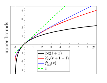
Figure 1: Plot of $f(x)=\log(1+x)$, its standard upper bound $h(x)=x$ and the majorizing functions obtained dividing the process in two steps, for $p=1/2$.

As we have already mentioned, it is possible to obtain better bounds by dividing the process into more stages. As an example, let us assume that we perform the cooling process from temperature $T+\Delta T$ (state 1) to temperature $T$ (state 4) in three steps, allowing the system to thermalize with reservoirs at temperatures $T+2\Delta T/3$ (state 2), $T+\Delta T/3$ (state 3), and finally with the environment at temperature $T$. The total entropy production obtained in this process can be shown to be

$$\Delta S^{Univ}_{1\rightarrow 3}=C\left[x\left(\dfrac{1}{3+2x}+\dfrac{1}{3+x}+\dfrac{1}{3}\right)-\log(1+x)\right],$$ (25)

so comparing this process with the two-step cooling process already studied (using $p=1/2$), we obtain that

$$\log(1+x)\leq f^{3}_{1/3,2/3}\leq f^{2}_{1/2}\leq x,$$ (26)

for $x>-1$, where

$$f^{3}_{1/3,2/3}=\dfrac{x(2x^{2}+18x+27)}{3(3+x)(3+2x)},$$ (27)

and

$$f^{2}_{1/2}=\dfrac{x(4+x)}{4+2x}.$$ (28)

This is illustrated in Fig. (2).

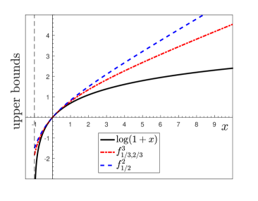
Figure 2: Comparison between the upper bounds for $\log(1+x)$ obtained partitioning the process into two and three steps.

Considering the heating process from temperature $T$ to temperature $T+\Delta T$ and following the same procedure, it is also possible to improve the lower-bound for $\log(1+x)$ given by Eq. (1). For instance, the reader may verify that if the system thermalizes with a reservoir at temperature $T+p\Delta T$ before reaching the final state, the following intermediate lower-bound can be deduced from the global entropy balance:

$$\dfrac{x}{1+x}\leq\dfrac{x[1+xp(2-p)]}{(1+x)(1+xp)}\equiv g^{2}_{p}(x)\leq\log(1+x),$$ (29)

with $x\geq-1$, and $0\leq p\leq 1$, see Fig. (3). The value of $p$ that maximizes $g^{2}_{p}(x)$ for each $x$ is the same that in the prevoius case, so substituting in (29), we obtain:

$$\dfrac{x}{1+x}\leq g^{2}_{p}(x)\leq 2\left(1-\dfrac{1}{\sqrt{x+1}}\right)\leq\log(1+x),$$ (30)

with $x\geq-1$, and $0\leq p\leq 1$.

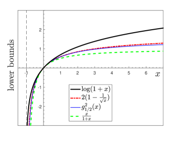
Figure 3: Plot of $f(x)=\log(1+x)$, its standard lower bound $j(x)=x/(1+x)$ and the minorizing functions obtained dividing the process in two steps, for $p=1/2$.

V Discussion and conclusions

The increase in entropy in every physical process establishes a connection between thermodynamics and the theory of algebraic inequalities that, in our opinion, deserves further exploration. In the first part of this work we have employed this connection to obtain a well known set of bounds for the logarithmic function. The inequalities are being generated from a physics postulate, which is remarkable since they are true independent of any thermodynamic considerations (and even if the second law turns out to be false). Whether this kind of reasoning represents a formal proof of these inequalities has been the subject of debate in the past, particularly in the context of derivations of the inequality between the arithmetic and geometric means Abriata ; Deakin ; Sidhu . Certainly, our view is critical about the logical consistency of thermodynamic proofs, since it is the maximization of entropy that assures that the imposed final state is, in fact, the equilibrium state. However, it is important to remark that we did not need to maximize the entropy to recognize the equilibrium state: it can be deduced from empirical considerations, such as the intuitive fact that the final temperature of a small system that exchanges energy with a thermal reservoir must coincide with the temperature of the reservoir. This implies that the underlying inequality associated with a particular process is never known or employed explicitly, but it is learned after the entropy balance is performed. In that sense, it is undeniable that the thermodynamic method constitutes a credible path towards the construction of true algebraic inequalities. Some of them may be well-known results, but others are possibly new. This has an intrinsic value regardless of whether the process employed can or cannot be considered a formal proof. Of course, if the readers feel uncomfortable, they can try to demonstrate the inequalities that arise from the thermodynamic analysis through traditional methods.

It is a well-known fact that in partitioning a thermodynamic process to bring it closer to the reversible limit, less entropy is produced. This implies that when performing the entropy analysis for the new process, a different inequality is obtained in which the terms involved are closer than those generated in the original inequality. As we have shown, this property allows us to improve the bounds for the logarithmic function found in Section II, but, of course, the validity of the method is not restricted to that particular function. In fact, bounds for a wide class of functions can be obtained and improved if, instead of using ideal gases and incompressible solids, other substances (even hypothetical, with a more complex dependence of the entropy on the other thermodynamic properties) are employed.

We believe that, in addition to their power to deduce new algebraic inequalities, the methods applied in this work have an interesting didactic value and can motivate students, especially those with a markedly mathematical profile, to delve into the study of thermodynamics.

Author Declarations

The author has no conflicts to disclose.

Appendix A Step processes and entropy production

The fact that the introduction of an intermediate equilibrium state decreases the total entropy production has been theoretically and experimentally demonstrated in several contexts. For example, in Ref. Gupta it is shown that if a linear spring is loaded to a total mass $M$ in $N$ equal steps, each time by a mass $M/N$, the total entropy production due to the energy dissipated to the environment by viscous friction is inversely proportional to the number of steps. The same dependence between the entropy production and N is observed in processes such as the charging of a capacitor, the compression of an ideal gas, or the heating of certain amount of water, when they are carried out in stages Gupta ; Heinrich ; Calkin . In what follows we show that for the cooling process of an incompressible solid, such as the one studied in section IV, the introduction of intermediate reservoirs reduces the entropy generation.

If the solid $A$ (initially at temperature $T_{1}$) is placed directly in thermal contact with a reservoir at temperature $T_{N}<T_{1}$, the global entropy variation once the new equilibrium state is reached is given by

$$\Delta S^{Univ}_{1\rightarrow N}=\Delta S^{A}_{1\rightarrow N}-\dfrac{\Delta U^{A}_{1\rightarrow N}}{T_{N}},$$ (31)

where $\Delta U^{A}_{1\rightarrow N}$ is the energy dissipated during the thermalization process. On the other hand, if the system first thermalizes with a set of reservoirs at temperatures $T_{2},T_{3},...T_{N-1}$ such that $T_{1}>T_{2}>...>T_{N-1}>T_{N}$, performing the entropy analysis for each process and adding the results we obtain that the new global entropy variation is:

$$\Delta S^{\prime Univ}_{1\rightarrow N}=\Delta S^{A}_{1\rightarrow N}-\sum_{j=1}^{N-1}\dfrac{\Delta U^{A}_{j\rightarrow j+1}}{T_{j+1}}$$ (32)

From Eqs. (31) and (32), and using that

$$\Delta U^{A}_{1\rightarrow N}=\sum_{j=1}^{N-1}\Delta U^{A}_{j\rightarrow j+1},$$ (33)

we obtain that the difference of the entropy variations is

$$\Delta S^{Univ}-\Delta S^{\prime Univ}=\sum_{j=1}^{N-2}\Delta U^{A}_{j\rightarrow j+1}\left(\dfrac{1}{T_{j+1}}-\dfrac{1}{T_{N}}\right).$$ (34)

Finally, noting that all energy variations $\Delta U^{A}_{j\rightarrow j+1}$ are negative (the solid releases energy) and that $T_{N}<T_{j+1}$ for all $j=1,...,N-1$, we have that each term in the right-hand side of Eq. (34) must be positive, so we conclude that

$$\Delta S^{\prime Univ}<\Delta S^{Univ},$$ (35)

and hence the new process must be closer to the reversible limit than the original.

Appendix B Thermodynamic derivation of the generalized Bernoulli’s inequality

Let us return to the analysis of the process suffered by a perfect gas contained in an adiabatic cylinder-piston device when a mass is suddenly added over the piston. It is important to remark that if the mass is not infinitesimal, the process followed by the gas will be non-quasi-static, and the internal pressure may be not be well-defined during the process. Nevertheless, since the external pressure is constant, the work performed by the gas can be calculated as Gislason :

$$W=\int_{V1}^{V2}P_{ext}dV=P_{2}(V_{2}-V_{1}).$$ (36)

The initial and final volumes can be expressed in terms of the pressures and temperatures using the equation of state for an ideal gas:

$$V_{2}-V_{1}=R\left[\dfrac{T_{2}}{P_{2}}-\dfrac{T_{1}}{P_{1}}\right].$$ (37)

Substituting Eqs. (36) and (37) into the first law for an adiabatic process:

$$\Delta U=-W,$$ (38)

and using that the internal energy is a function of the temperature only Cengel :

$$\Delta U=c_{v}\Delta T,$$ (39)

we obtain that

$$c_{v}\left(T_{2}-T_{1}\right)=-R\left[T_{2}-\dfrac{P_{2}T_{1}}{P_{1}}\right].$$ (40)

From the above equation, and using that for an ideal gas $c_{p}-c_{v}=R$, we find the temperature of the final state:

$$T_{2}=\left[\dfrac{c_{v}}{c_{p}}+\dfrac{R{P_{2}}}{c_{p}P_{1}}\right]T_{1},$$ (41)

which can be expressed as:

$$T_{2}=T_{1}\left(1+\delta x\right),$$ (42)

where $x$ and $\delta$ are given by Eq. (11).

Now we are in position to analyze the process from the perspective of the second law. Since the entropy of the environment does not change, the total entropy production coincides with the entropy variation of the gas, which can be evaluated from the equation:

$$\Delta S^{gas}_{1\rightarrow 2}=c_{P}\log\left(\dfrac{T_{2}}{T_{1}}\right)-R\log\left(\dfrac{P_{2}}{P_{1}}\right),$$ (43)

which, combined with Eq. (42) and the relation $P_{2}/P_{1}=1+x$, gives

$$\dfrac{\Delta S^{Univ}_{1\rightarrow 2}}{c_{p}}=\log(1+\delta x)-\delta\log(1+x)\geq 0,$$ (44)

from which the upper bound

$$(1+x)^{\delta}\leq 1+\delta x$$ (45)

is obtained. It is easy to verify that the conditions $x>-1$ and $0<\delta<1$ are satisfied on noting that $P$ is a non-negative quantity and that $R<c_{P}$ for an ideal gas. However, for the proof to be valid for any values of $x$ and $\delta$ in the described ranges, we must assume the existence of perfect gases with all values of $\delta$ in $(0,1)$, and that the gas is still ideal even for large values of pressure, situation in which the hypothesis that the molecules are not-interacting ceases to be reasonable.

Regarding the lower bound, it can be found by analyzing the process $2\rightarrow 3$ undergone by the gas after removing the load from the piston. Following the same procedure, we obtain that the new equilibrium state is defined by the following properties:

$$P_{3}=P_{1},\hskip 5.69046ptT_{3}=T_{2}\left[\dfrac{1+x(1-\delta)}{1+x}\right]$$ (46)

so the entropy created during the expansion satisfies

$$\dfrac{\Delta S^{Univ}_{2\rightarrow 3}}{C_{p}}=\log\left[\dfrac{1+x(1-\delta)}{1+x}\right]+\delta\log(1+x)\geq 0,$$ (47)

a result that proves the left inequality in Eq. (10).

References

- (1) E. R. Love, Some logarithm inequalities, The Mathematical Gazette 64, 427, pp. 55–57 (1980).
- (2) F. Topsok, Some bounds for the logarithmic function, Inequality theory and applications 4 (2006).
- (3) C. Chesneau and Y. J. Bagul, New Sharp Bounds for the Logarithmic Function, Electronic Journal of Mathematical Analysis and Applications 8, 1 140–145 (2020).
- (4) P. G. Tait, Physical proof that the geometric mean of any number of quantities is less than the arithmetic mean, Proc. Roy. Soc. Edin. 6, 309 (1868/9); reprinted in Scientific Papers 1, 83 (1898).
- (5) A. Sommerfeld, Thermodynamics and statistical mechanics (Academic Press, New York, 1964).
- (6) E. D. Cashwell and C. J. Everett, The means of order t and the laws of thermodynamics, Am. Math. Monthly 74, 271–274 (1967).
- (7) P. T. Landsberg, A thermodynamic proof of the inequality between arithmetic and geometric means, Phys. Lett. A 67, 1 (1978).
- (8) R. J. Tykodi, Using model systems to demonstrate instances of mathematical inequalities, Am. J. Phys. 64 5, 644–648 (1996).
- (9) L. Wang, Second law of thermodynamics and arithmetic-mean–geometric-mean inequality, Internat. J. Modern Phys. B, 13 (21-22):2791–2793 (1999).
- (10) C. Graham and T. Tokieda, An Entropy Proof of the Arithmetic Mean–Geometric Mean Inequality, The American Mathematical Monthly, 127:6, 545-546 (2020).
- (11) R. S. Johal, Optimal performance of heat engines with a finite source or sink and inequalities between means, Phys. Rev. E 94, 012123 (2016).
- (12) Y.A. Cengel, and M.A. Boles, Thermodynamics: An Engineering Approach, 4th edition (McGraw-Hill, New York, 2001).
- (13) G. J. Van Wylen G.J. and R.E Sonntag, Fundamentals of Classical Thermodynamics, 1st edition (John Wiley and Sons, New York, 1965).
- (14) Y.-C. Li and C.-C. Yeh, Some equivalent forms of Bernoulli’s inequality: A survey, Applied Mathematics, 4, 7 (2013).
- (15) L.R. Berrone, C.D. Galles, Comment on “Using model systems to demonstrate instances of mathematical inequalities”, Am. J. Phys. 66 (87-88) (1998).
- (16) . P. Abriata, Comment on a thermodynamical proof of the inequality between arithmetic and geometric mean, Phys. Lett. A 71, 309–310 (1979).
- (17) M. A. B. Deakin and G. J. Troup, The logical status of thermodynamic proofs of mathematical theorems, Phys. Lett. A 83 6, 239–240 (1981).
- (18) S. S. Sidhu, On thermodynamic proof of mathematical results, Phys. Lett. A 76, 107–108 (1980).
- (19) C. E. Mungan, Damped oscillations of a frictionless piston in an adiabatic cylinder enclosing an ideal gas. Eur. J. Phys. 38, 035102 (2017).
- (20) E. A. Gislason, N. C. Craig, Pressure-volume integral expressions for work in irreversible processes., J. Chem. Educ. 84, 499 (2007).
- (21) V. K. Gupta, G. Shanker and N. K. Sharma, Reversibility and step processes: an experiment for the undergraduate laboratory, Am. J. Phys. 52 945–7 (1984).
- (22) M. G. Calkin and D. Kiang, Entropy change and reversibility, Am. J. Phys. 51, 78 (1983).
- (23) F. Heinrich, Entropy change when charging a capacitor: A demonstration experiment, Am. J. Phys. 54, 742–744 (1986).