Three-dimensional accelerating AdS black holes in $F(R)$ gravity

Abstract

Considering a three-dimensional $C-$metric, we obtain the exact accelerating black holes in the $F(R)$ theory of gravity coupled with and without a matter field. First, we extract uncharged accelerating AdS black hole solutions in $F(R)$ gravity. Then, we study the effects of various parameters on metric function, roots, and the temperature of these black holes. The temperature is always positive for the radii less than $\frac{1}{\alpha}$, and it is negative for the radii more than $\frac{1}{\alpha}$. We extend our study by coupling nonlinear electrodynamics as a matter filed to $F(R)$ gravity to obtain charged black holes in this theory. Next, we evaluate the effects of different parameters such as the electrical charge, accelerating parameter, angular, $F(R)$ gravity, and scalar curvature on the obtained solutions, roots, and temperature of three-dimensional charged accelerating AdS black holes. The results indicate that there is a root in which it depends on various parameters. The temperature of these black holes is positive after this root.

I Introduction

The accelerating black hole has some exciting properties among other black holes. The spacetime of the accelerating black holes is extracted from $C-$metric Kinnersley1970 ; Plebanski1976 ; Griffiths2006 . A conical deficit angle along one polar axis of this black hole provides the force driving acceleration. To understand them, one can imagine that something similar to the $C-$metric can describe a black hole accelerated by an interaction with a local cosmological medium. The asymptotic behavior of the accelerating black holes described by $C-$metric depends on various parameters, which lead to an accelerating horizon and complicate the asymptotic structure. In this regard, some interesting properties of the (un)charged accelerating (non)rotating (A)dS black holes have been studied in Refs. AC1 ; AC3 ; AC4 ; AC5 ; AC6 ; AC7 ; AC8 ; AC9 ; AC11 ; AC12 ; AC13 ; AC14 ; AC15 ; AC16 .

The classical electromagnetic theory of Maxwell is a widely used fundamental theory. However, a singularity at the position of the point charge leads to an infinite self-energy, which is a fundamental problem of Maxwell’s theory. To overcome this problem, Born and Infeld introduced a nonlinear electromagnetic (NED) field in 1934 BornII . Then, numerous models of NED were developed (see Refs. NED1 ; NED2 ; NED3 ; NED4 ; NED5 , for more details). Power-Maxwell invariant (PMI) theory is one of these special classes of NED NED2 , in which its Lagrangian is an arbitrary power of Maxwell Lagrangian PMI . PMI reduces to a linear Maxwell field with considering a special value, and also it can remove the singularity at the position of the point charge PMII ; PMIII . There is an interesting property for PMI, and it is related to conformal invariance. In other words, the energy-momentum tensor of PMI is traceless when the power of the Maxwell invariant is a quarter of spacetime dimensions, which leads to conformal invariance. In this case, PMI is known as conformal invariant Maxwell (CIM). This idea is related to taking advantage of the conformal symmetry to construct the analogs of the four-dimensional Reissner-Nordström black holes with an inverse square electric field in arbitrary dimensions NED2 ; PMI .

On the other hand, the string theory partition function contains higher-curvature terms in the IR limit such that considering Kaluza–Klein reductions can lead to NED coupling to the Einstein sector Gibbons2011 . In addition, nonlinear kinetic terms for the vector fields also appear in the quantization of string actions Fradkin1985 . So, NED theories introduced as an alternative to Maxwell electrodynamics to solve problems in quantum electrodynamics, can be considered in the duality and allows extending the possible holographic field theories. Moreover, there are interesting motivations of NED for applications in gravity, cosmology, and CMT as well Sorokin2022 . For example; i) NED coupled to gravity have been used to construct regular black hole solutions regular1 ; regular2 ; regular3 ; regular4 ; regular5 ; regular6 , ii) to create cosmological models, which might avoid initial Big-Bang singularities BigB1 ; BigB2 , iii) to mimic dark energy and generate an accelerated expansion of the universe NonUni1 ; NonUni2 ; NonUni3 , iv) AdS/CFT correspondence and gravity/CMT holography AdSCMT1 ; AdSCMT2 ; AdSCMT3 ; AdSCMT4 ; AdSCMT5 . Also, the effects of NED on the thermodynamics properties of black holes have been studied in some literature NEDBH1 ; NEDBH2 ; NEDBH3 ; NEDBH4 ; NEDBH5 ; NEDBH6 ; NEDBH7 .

An accelerated universe expansion was confirmed by various observational evidence, for example, the luminosity distance of Supernovae type Ia. Identifying the cause of this late-time acceleration is a challenging problem from the cosmology point of view. Among candidates that can explain it, $F(R)$ gravity as a modified theory of gravity attracted significant attention because of specific properties. $F(R)$ theory of gravity is the straightforward modification of Einstein’s gravity, which can describe some phenomena from various points of view. The gravitational action in this theory is a general function of $R$ F(R)I ; F(R)II ; F(R)III ; F(R)IV . This theory may give a unified description of early-time inflation InflationI ; InflationII . It may describe the structure formation of the Universe without considering dark energy or dark matter. Moreover, $F(R)$ gravity coincides with Newtonian and post-Newtonian approximations Capozziello2005 ; Capozziello2007 . It is worth mentioning that this theory of gravity may extract the whole sequence of the Universe’s evolution epochs: inflation, radiation/matter dominance, and dark energy.

The conjectured equivalence of string theory on AdS spaces and super-conformal gauge theories living on the boundary of AdS has led to an increasing interest in asymptotically AdS black holes AdS1 ; AdS2 ; AdS3 . This interest is based on the fact that the classical super-gravity black hole solution can furnish important information on the dual gauge theory in the large N limit (in which N denotes the rank of the gauge group). A standard example of this is the well-known Schwarzschild AdS black hole, whose thermodynamics was studied by Hawking and Page in Ref. HawkingP1983 . They discovered a phase transition from thermal AdS space to a black hole phase, as the temperature increases. The Hawking-Page phase transition was then reconsidered by Witten in the spirit of the AdS/CFT correspondence Witten1998 . In this regard, the study of the thermodynamics of AdS black holes has been extended in various theories of gravity with linear and nonlinear Maxwell fields ThAdS1 ; ThAdS2 ; ThAdS3 ; ThAdS4 ; ThAdS5 ; ThAdS6 ; ThAdS7 ; ThAdS8 ; ThAdS9 ; ThAdS10 ; ThAdS11 .

Until now, all extant $C-$metrics describing accelerating black holes are obtained in the context of Einstein’s gravity for three and four dimensions of spacetime with or without linear and nonlinear electrodynamics fields. For example, the asymptotically AdS accelerated black holes and their thermodynamic properties in the presence of the ModMax electrodynamics have been studied in Ref. Barrientos2022 . This research opened a window towards studying radiative spacetimes in NED regimes, as well as raised new challenges for their corresponding holographic interpretation Barrientos2022 . Also, by considering this NED (MadMax) a novel $C-$metric which describes accelerated AdS black holes is given in Ref. Hale2023 . On the other hand, the investigations on Einstein’s gravity solutions in three-dimensional spacetime provide a powerful background to study the physical properties of gravity and examine its viability in lower spacetime dimensions. Especially, it can be simulated as a toy model of quantum gravity. This property was discovered after the arguments presented connecting the possible links between three-dimensional gravitation and the Chern-Simons theory Achucarro1986 ; Witten1986 . Considering Einstein’s gravity, the uncharged accelerating black holes in three-dimensional spacetime have been extracted in Refs. BTZAcI ; BTZAcII ; BTZAcIIb ; BTZAcIII . The first solution of the accelerating BTZ black hole is given by Astorino in Ref. BTZAcI . Then, Xu et al. studied it with more detail in Refs. BTZAcII ; BTZAcIIb . In this regard, Arenas-Henriquez et al. evaluated the accelerating systems in $(2+1)-$dimensional spacetime, and found three exciting classes of geometry by studying holographically their physical parameters BTZAcIII . Moreover, by coupling Einstein’s gravity and CIM, the exact charged accelerating BTZ black hole solutions are obtained in Ref. EslamPanahArXiv .

It is interesting to find (un)charged accelerating black hole solutions in modified theories of gravity, such as $F(R)$ gravity. Generally, the field equations of $F(R)$ theory coupled to a matter field is complicated, and hence it is not easy to find exact analytical accelerating black hole solutions. In this regard, by considering $F(R)$ gravity, the charged accelerating black hole solutions in four-dimensional spacetime had been obtained in Ref. ZhangMann2019 . However, there is no three-dimensional (un)charged accelerating black hole solution in the context of $F(R)$ gravity. For this purpose, by coupling $F(R)$ gravity with CIM, we will find (un)charged accelerating black hole solutions in this theory known as $F(R)$-CIM gravity.

II Uncharged Solutions

Here, we consider $F(R)$ gravity to extract accelerating black hole solutions in three-dimensional spacetime. We consider the action of $F(R)$ gravity in the following form

$$\mathcal{I}=\frac{1}{16\pi}\int_{\partial\mathcal{M}}d^{3}x\sqrt{-g}F(R),$$ (1)

where $F(R)=R+f\left(R\right)$, which $R$ is scalar curvature (Ricci scalar), and $f\left(R\right)$ is an arbitrary function of scalar curvature $R$. In the above action, we considered $G=1$.

Varying the action (1) with respect to the gravitational field $g_{\mu\nu}$ leads to

$$R_{\mu\nu}\left(1+f_{R}\right)-\frac{g_{\mu\nu}F(R)}{2}+\left(g_{\mu\nu}\nabla^{2}-\nabla_{\mu}\nabla_{\nu}\right)f_{R}=0,$$ (2)

where $f_{R}=\frac{df(R)}{dR}$.

We consider the following three-dimensional $C-$metric to extract the accelerating black hole solutions as it was introduced in Refs. BTZAcII ; BTZAcIIb

$$ds^{2}=\frac{1}{\mathcal{K}^{2}\left(r,\theta\right)}\left[-g(r,\theta)dt^{2}+\frac{dr^{2}}{g(r,\theta)}+r^{2}d\theta^{2}\right],$$ (3)

where $\mathcal{K}\left(r,\theta\right)=\alpha r\cosh\left(\sqrt{m-k}\theta\right)-1$, which is called the conformal factor. Also, $k$ is a topological constant that can be $\pm 1$ or $0$. In addition, $g(r,\theta)$ is a metric function, which we have to find it. The coordinates of $t$ and $r$ in the metric, respectively, are in the ranges $-\infty<t<\infty$ and $0\leq r<\infty$. Due to the lack of translational symmetry in $\theta$ (in the presence of the conformal factor), we seem to have no reason to restrict it to be in $\left[-\pi,\pi\right]$. So, we consider $\theta$ in the range $-\pi\leq\theta\leq\pi$ (more details are given in Ref. BTZAcII ; BTZAcIIb ).

It is notable that in three-dimensional spacetime, we may find two methods for understanding if our metric is under acceleration or not. These methods are:

(i) a domain wall (which is studied by Arenas-Henriquez et al. in Ref. BTZAcIII ).

(ii) by calculating the proper acceleration of spacetime (which is discussed in Refs. BTZAcI ; BTZAcII ; BTZAcIIb ).

Here, we consider the method (ii) and calculate the proper acceleration of the mentioned spacetime (Eq. (3)). Considering a static observer in spacetime as

$$x^{\mu}\left(\lambda\right)=\left(\lambda\frac{\mathcal{K}}{\sqrt{g(r,\theta)}},r,\theta\right),$$ (4)

where $\lambda$ is the proper time. Also, proper velocity is defined $u^{\mu}=\frac{dx^{\mu}}{d\lambda}$. Using Eq. (4) and the definition of the proper velocity, we can get $u^{\mu}$ as

$$u^{\mu}\left(\lambda\right)=\left(\frac{\mathcal{K}}{\sqrt{g(r,\theta)}},0,0\right).$$ (5)

We will calculate the proper acceleration after extracting the metric function ($g(r,\theta)$).

In the following, we want to obtain the solutions for the constant scalar curvature (i.e., $R=R_{0}=constant$) in three-dimensional spacetime. The trace of Eq. (2) yields

$$R_{0}\left(1+f_{R_{0}}\right)-\frac{3}{2}\left(R_{0}+f(R_{0})\right)=0,$$ (6)

where $f_{R_{0}}=$ $f_{R_{\left|{}_{R=R_{0}}\right.}}$, and the solution for $R_{0}$ gives

$$R_{0}=\frac{3f(R_{0})}{2f_{R_{0}}-1}\equiv 6\Lambda<0.$$ (7)

Since it was shown that in three-dimensional dS spacetime, classical black holes do not exist Emparan , so we consider the negative value for $R_{0}$ (or the cosmological constant) in this work.

Substituting the equation (7) into Eq. (2), we can obtain the equations of motion in $F(R)$ gravity in the following form

$$R_{\mu\nu}\left(1+f_{R_{0}}\right)-\frac{g_{\mu\nu}R_{0}\left(1+f_{R_{0}}\right)}{3}=0.$$ (8)

Considering the metric (3), and the field equation of $F(R)$ gravity (8), one can write the following field equations

$$eq_{tt} = eq_{rr}=\left(\mathcal{K}+1\right)^{2}\left(rg^{\prime\prime}-2g^{\prime}+\frac{2g}{r}\right)+rg^{\prime\prime}-2\left(\mathcal{K}+1\right)\left(rg^{\prime\prime}-\frac{g^{\prime}}{2}-\frac{g}{r}\right)$$ (9)

$$+g^{\prime}+\frac{2rR_{0}}{3},$$

$$eq_{\theta\theta} = g^{\prime}-\frac{\left(\mathcal{K}+1\right)\left(rg^{\prime}-2g\right)}{r}+\frac{rR_{0}}{3},$$ (10)

where $eq_{tt}$, $eq_{rr}$ and $eq_{\theta\theta}$, respectively, are related to components of $tt$, $rr$ and $\theta\theta$ of Eq. (8). Also, in the above equations $\mathcal{K}=\mathcal{K}\left(r,\theta\right)$, $g=g\left(r,\theta\right)$, $g^{\prime}=\frac{\partial g\left(r,\theta\right)}{\partial r}$, and $g^{\prime\prime}=\frac{\partial^{2}g\left(r,\theta\right)}{\partial r^{2}}$. Now we are in a position to obtain an exact solution from Eqs. (9) and (10). After some calculations, one can get the following metric function

$$g(r,\theta)=C\left(\theta\right)\mathcal{K}^{2}-\frac{\left(2\mathcal{K}+1\right)r^{2}R_{0}}{6\left(\mathcal{K}+1\right)^{2}},$$ (11)

where the above solution (11) satisfies all components of the field equation (8). Also, $C\left(\theta\right)$ is an integration constant-dependent and depends on $\theta$. It is necessary to mention that the solutions in any modified theories of gravity must reduce to the famous solutions in Einstein’s gravity. The obtained solution (11) does not reduce to the famous BTZ black hole solutions when $\alpha=0$. Using a choice for $C\left(\theta\right)$, we can remove this problem. This choice is

$$C\left(\theta\right)=k-m-\frac{R_{0}}{6\alpha^{2}\cosh^{2}\left(\sqrt{m-k}\theta\right)},$$ (12)

and by replacing Eq. (12) into the solution (11), we obtain accelerating black holes in $F(R)$ gravity in the following form

$$g(r,\theta)=\left(k-m\right)\mathcal{K}^{2}-\frac{r^{2}R_{0}}{6},$$ (13)

where in the absence of the acceleration parameter (i.e., $\alpha=0$), the solution (13) reduces to the BTZ black hole in $F(R)$, as we expected. It is notable that for recovering the famous static BTZ black hole and to respect the signatures of spacetime (3), we have to restrict $m>k$.

Now we are in a position to get the proper acceleration. After some calculations, we can obtain the proper acceleration (which is defined as $a^{\mu}=u^{\nu}\nabla_{\nu}u^{\mu}$) for the observer in the distance as

$$a^{\mu}a_{\mu}=\frac{R_{0}^{2}\left[6\left(k-m\right)\alpha^{2}-R_{0}\right]}{\left(6\alpha^{2}\left(k-m\right)\cosh^{2}\left(\sqrt{m-k}\theta\right)-R_{0}\right)^{2}},$$ (14)

in which indicates, $\alpha$ is proportional (but not equal) to the magnitude $|a|$ of the proper acceleration (see Refs. BTZAcI ; BTZAcII ; BTZAcIIb for more details). So, we call $\alpha$ as an acceleration parameter.

Considering the solution (13), we want to find the Kretschmann scalar of the spacetime (3) which leads to

$$R_{\alpha\beta\gamma\delta}R^{\alpha\beta\gamma\delta}=\frac{R_{0}^{2}}{3},$$ (15)

where indicates that this scalar does not diverge at $r=0$. Indeed, a curvature singularity does not exist at $r=0$, but there is a conical singularity for this spacetime.

In the following, we find the real roots of the metric function (13). In this regard, we solve the metric function (13) and get two roots in the following forms

$$r_{root_{\pm}}=\frac{2\left[3\alpha\left(m-k\right)\left(\mathcal{B}^{2}+1\right)\pm\mathcal{B}\sqrt{6R_{0}\left(k-m\right)}\right]\mathcal{B}}{2R_{0}\mathcal{B}^{2}+3\alpha^{2}\left(m-k\right)\left(\mathcal{B}^{4}+2\mathcal{B}^{2}+1\right)},$$ (16)

where $\mathcal{B}=\exp\left(\sqrt{m-k}\theta\right)$. To have the real root for the metric function (13), we have to respect $R_{0}<0$, since $m>k$.

Here, we plot $g(r,\theta)$ versus $r$ in Fig. 1. As shown in Fig. 1, there is at least a root. In order to investigate the effects of various parameters on the roots, we plotted four diagrams in Fig. 1. Each diagram indicates that each parameter how affects the roots.

Our results indicate that with increasing mass, the radii of the accelerating BTZ AdS black holes increase (see the dotted, dashed, and dotted-dashed lines in the up-left panel in Fig. 1). However, there is a critical value for mass ($m_{critical}$) which by increasing it more than a critical value, i.e., $m>m_{critical}$, these black holes include two roots. The small root is related to the event horizon, and the large root belongs to the cosmological horizon. The effect of $\theta$ in the up-right panel in Fig. 1 reveals that by increasing $\theta$, the radius of the black hole decreases. In addition, there is a critical value for $\theta$ ($\theta_{critical}$) which by increasing this quantity more than a critical value, i.e., $\theta>\theta_{critical}$, these black holes include two horizons (event and cosmological horizons). There is the same behavior for the acceleration parameter. Indeed, by increasing $\alpha$, the radius of the black hole decreases. Also, there is a critical value for $\alpha>\alpha_{critical}$. In this case, the black holes have two roots. The small root is related to the event horizon, and the large root belongs to the cosmological horizon (see the down-left panel in Fig. 1). Also, we encounter small black holes when the absolute value of the Ricci scalar $\left|R_{0}\right|$ increase (see the down-right panels in Fig. 1).

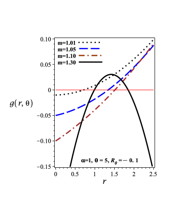
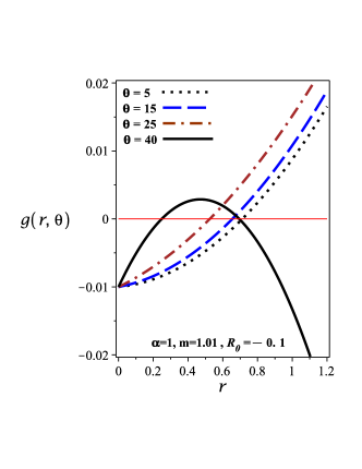
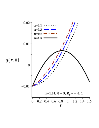
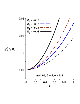
Figure 1: The metric function $g(r,\theta)$ versus $r$ for $k=1$ and different values of the parameters.

Considering the obtained metric function, the asymptotical behavior of the mentioned spacetime depends on the parameters of this theory, which include $\alpha$, $k$, $m$, and $R_{0}$. As a result, the obtained spacetime is not exactly asymptotically AdS due to different parameters in the obtained metric function.

Here, we study the effects of different parameters on the temperature of these black holes. For this purpose, we first have to get the black hole’s temperature. Using the Hawking temperature in the following form

$$T_{H}=\frac{\kappa}{2\pi},$$ (17)

where $\kappa$ is the surface gravity in the form $\kappa=\sqrt{-\frac{1}{2}\left(\nabla_{\mu}\chi_{\nu}\right)\left(\nabla^{\mu}\chi^{\nu}\right)}$. Also, $\chi=\partial_{t}$ is the Killing vector. Considering the metric (3), we get the surface gravity as

$$\kappa=\left.\frac{1}{2}\left(\frac{\partial g\left(r,\theta\right)}{\partial r}\right)\right|_{r=r_{+}}.$$ (18)

Using the above equation and the metric function (13), we are in a position to get the Hawking temperature. To obtain the temperature of these black holes, we have to express the mass ($m$) in terms of the radius of event horizon $r_{+}$, the accelerating parameter $\alpha$, and $R_{0}$ in the following form

$$m=k-\frac{r_{+}^{2}R_{0}}{6\left(\alpha r_{+}-1\right)^{2}},$$ (19)

which we extract the above equation by considering $g\left(r,\theta\right)=0$. Notably, to get the exact form (19), we suppose $\theta=0$ in the metric function (13).

Substituting the mass (19) within the equations (18) and then (17), one can calculate the Hawking temperature

$$T_{H}=\frac{r_{+}R_{0}}{12\pi\alpha\left(\alpha r_{+}-1\right)}.$$ (20)

In the context of black holes, it is argued that the root of temperature ($T=0$) represents a borderline between physical ($T>0$) and non-physical ($T<0$) black holes Temperature . To study the behavior of temperature of these black holes, we evaluate their roots. There is no root for the temperature. On the other hand, to have a positive temperature, we must respect $\alpha r_{+}<1$ because $R_{0}<0$. By considering $\alpha r_{+}<1$, the temperature increases by increasing (decreasing) the value of $\left|R_{0}\right|$ ($\alpha$).

III Charged Solutions

In order to extract charged accelerating black hole solutions in three-dimensional spacetime, we add the CIM field as a source (which leads to traceless energy-momentum tensor) to $F(R)$ gravity. The action of $F(R)$ gravity coupled to the PMI field is given HendiES2014

$$\mathcal{I}=\frac{1}{16\pi}\int_{\partial\mathcal{M}}d^{3}x\sqrt{-g}\left[F(R)+L\left(\mathcal{F}\right)\right],$$ (21)

where $L\left(\mathcal{F}\right)=\left(-\mathcal{F}\right)^{s}$, and for CIM filed $s=\frac{3}{4}$ (i.e., $L\left(\mathcal{F}\right)=\left(-\mathcal{F}\right)^{\frac{3}{4}}$). $\mathcal{F}=$ $F_{\mu\nu}F^{\mu\nu}$ is the Maxwell invariant ($F_{\mu\nu}=\partial_{\mu}A_{\nu}-\partial_{\nu}A_{\mu}$ is the electromagnetic tensor field, and $A_{\mu}$ is the gauge potential). Varying the action (21) with respect to the gravitational field $g_{\mu\nu}$, and the gauge field $A_{\mu}$, lead to

$$R_{\mu\nu}\left(1+f_{R}\right)-\frac{g_{\mu\nu}F(R)}{2}+\left(g_{\mu\nu}\nabla^{2}-\nabla_{\mu}\nabla_{\nu}\right)f_{R} = 8\pi\mathrm{T}_{\mu\nu},$$ (22)

$$\partial_{\mu}\left(\sqrt{-g}\mathcal{F}^{-\frac{1}{4}}F^{\mu\nu}\right) = 0,$$ (23)

where the energy-momentum tensor ($\mathrm{T}_{\mu\nu}$) in the presence of CIM for three-dimensional spacetime can be written

$$\mathrm{T}_{\mu\nu}=\frac{3}{2}F_{\mu\rho}F_{\nu}^{\rho}\left(-\mathcal{F}\right)^{-\frac{1}{4}}+\frac{1}{2}g_{\mu\nu}\left(-\mathcal{F}\right)^{\frac{3}{4}}.$$ (24)

We obtain the equations of motion in $F(R)$-CIM gravity by replacing the equation (7) into Eq. (22), which leads to

$$R_{\mu\nu}\left(1+f_{R_{0}}\right)-\frac{g_{\mu\nu}R_{0}\left(1+f_{R_{0}}\right)}{3}=8\pi\mathrm{T}_{\mu\nu}.$$ (25)

Notably, the assumption of a traceless energy-momentum tensor (a result of CIM) is essential for deriving exact black hole solutions in $F(R)$ gravity coupled to the matter field in metric formalism.

According to this fact that we look for black hole solutions with a radial electric field, so the gauge potential is given by $A_{\mu}=h(r)\delta_{\mu}^{0}$ (i.e., $A_{\mu}=\left[h(r),0,0\right]$). Using the introduced metric in the equation (3) and the mentioned gauge potential, one can show that Eq. (23) reduces to

$$\mathcal{K}^{4}\left(r,\theta\right)\left(rh^{\prime\prime}(r)+2h^{\prime}(r)\right)=0,$$ (26)

solving Eq. (26), one can find

$$h(r)=-\frac{q}{r},$$ (27)

where $q$ is an integration constant related to the electric charge. Our calculation for obtaining the electric field leads to $F_{tr}=-F_{rt}=\partial_{t}A_{r}-\partial_{r}A_{t}=\frac{q}{r^{2}}$, where it shows that the electric field in three-dimensional spacetime is the inverse square of $r$ (similar to four-dimensional spacetime). It is notable that we restrict ourselves to $\alpha r\cosh\left(\sqrt{m-k}\theta\right)\neq 1$ to obtain the equation (27).

Considering the metric (3), the electric field, and the field equation of $F(R)$-CIM gravity (25), one can write the following field equations

$$eq_{tt} = eq_{rr}=\frac{\left(2q^{2}\right)^{\frac{3}{4}}\mathcal{K}^{3}}{2\left(1+f_{R_{0}}\right)r^{2}}-\frac{\left(\mathcal{K}+1\right)^{2}\left(r^{2}g^{\prime\prime}-2rg^{\prime}+2g\right)}{r}+\frac{2\left(\mathcal{K}+1\right)\left(r^{2}g^{\prime\prime}-\frac{rg^{\prime}}{2}-g\right)}{r}$$ (28)

$$-rg^{\prime\prime}-g^{\prime}-\frac{2rR_{0}}{3},$$

$$eq_{\theta\theta} = \frac{\left(2q^{2}\right)^{\frac{3}{4}}\mathcal{K}^{3}}{2\left(1+f_{R_{0}}\right)r^{2}}+g^{\prime}+\frac{rR_{0}}{3}-\frac{\left(\mathcal{K}+1\right)\left(rg^{\prime}-2g\right)}{r},$$ (29)

and we get the metric function as

$$g(r,\theta)=C\left(\theta\right)\mathcal{K}^{2}-\frac{\left(2\mathcal{K}+1\right)r^{2}R_{0}}{6\left(\mathcal{K}+1\right)^{2}}-\frac{\left(2q^{2}\right)^{\frac{3}{4}}\mathcal{K}^{2}}{2r\left(1+f_{R_{0}}\right)},$$ (30)

where the solution (30) satisfies all components of the field equation (25). In order to recover the famous solutions in Einstein’s gravity, we consider

$$C\left(\theta\right)=k-m-\frac{R_{0}}{6\alpha^{2}\cosh^{2}\left(\sqrt{m-k}\theta\right)}-\frac{\left(2q^{2}\right)^{\frac{3}{4}}\alpha\cosh\left(\sqrt{m-k}\theta\right)}{4\left(1+f_{R_{0}}\right)},$$ (31)

and by replacing Eq. (31) into the solution (30), we obtain charged accelerating black hole solutions in $F(R)$ gravity

$$g(r,\theta)=\left(k-m\right)\mathcal{K}^{2}-\frac{\left(2q^{2}\right)^{\frac{3}{4}}\mathcal{K}^{2}\left(\mathcal{K}+3\right)}{4\left(1+f_{R_{0}}\right)r}-\frac{r^{2}R_{0}}{6},$$ (32)

where we restrict ourselves to $f_{R_{0}}\neq-1$. Indeed, to have physical solutions, we should restrict ourselves to $f_{R_{0}}\neq-1$. In the absence of the acceleration parameter (i.e., $\alpha=0$), the solution (32) reduces to the BTZ black hole in $F(R)$-CIM gravity HendiES2014 in the following form, as we expected

$$g(r)=k-m-\frac{\left(2q^{2}\right)^{\frac{3}{4}}}{2\left(1+f_{R_{0}}\right)r}-\frac{r^{2}R_{0}}{6}.$$ (33)

Considering the introduced spacetime in Eq. (3), with the metric function (32), we obtain the Kretschmann scalar as $R_{\alpha\beta\gamma\delta}R^{\alpha\beta\gamma\delta}=\frac{R_{0}^{2}}{3}+\frac{3\sqrt{2}q^{3}\mathcal{K}^{6}}{\left(1+f_{R_{0}}\right)r^{6}}$, where $\underset{r\longrightarrow 0}{\lim}R_{\alpha\beta\gamma\delta}R^{\alpha\beta\gamma\delta}\longrightarrow\infty$, and indicates this scalar diverge at $r=0$. So, there is a curvature singularity at $r=0$.

In order to investigate the effects of various parameters on the roots of the metric function (32), we plotted six diagrams in Fig. 2. Each diagram indicates that each parameter how affects the roots. The up-left panel in Fig. 2 shows that higher-charged accelerating BTZ black holes have large radii. However, we encounter small black holes when the parameter of $F(R)$ (i.e., $f_{0}$) and the absolute value of the Ricci scalar $\left|R_{0}\right|$ increase (see up-middle and up-right panels in Fig. 2). Our results in the down panels of Fig. 2 show that there are the critical values for parameters of $m$, $\theta$, and $\alpha$. As shown in the down-left panel in Fig. 2, massive charged accelerating black holes have large radii. However, by increasing mass more than a critical value (i.e., $m>m_{critical}$), our solutions include two roots. Indeed, The small root is related to the event horizon, and the large root belongs to the cosmological horizon. We encounter small black holes when $\theta$ and $\alpha$ increase. In other words, the radius of the black hole decreases by increasing $\theta$ and $\alpha$. Moreover, there are two roots when $\theta$ and $\alpha$ increase more than a critical value (see continuous lines in the down-middle and down-right panels in Fig. 2).

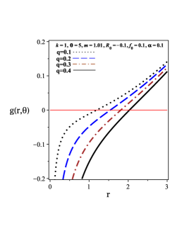
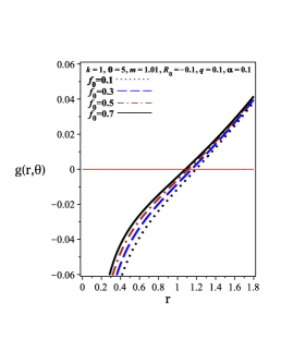
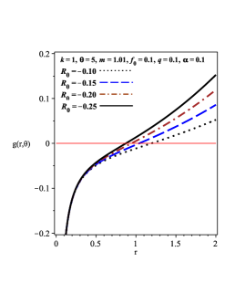
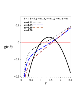
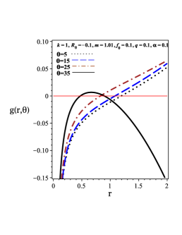
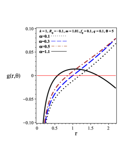
Figure 2: The metric function $g(r,\theta)$ versus $r$ for different values of the parameters.

Notably, the asymptotical behavior of the mentioned spacetime is dependent on the parameters of this theory ($k$, $m$, $R_{0}$, $q$, and $f_{R_{0}}$).

Using the Hawking temperature in Eq. (17), and the metric function (32), we are in a position to get the Hawking temperature of these black holes. We express the mass ($m$) in terms of the radius of the event horizon $r_{+}$, the accelerating parameter $\alpha$, $R_{0}$ and the charge $q$ in the following form

$$m=k-\frac{r_{+}^{2}R_{0}}{6\left(\alpha r_{+}-1\right)^{2}}-\frac{\left(2q^{2}\right)^{\frac{3}{4}}\left(\alpha r_{+}+2\right)}{4\left(1+f_{R_{0}}\right)r_{+}},$$ (34)

which we suppose $\theta=0$ in the metric function (32), to get the exact form (34).

Substituting the mass (34) within the equation (17), one can calculate the Hawking temperature

$$T_{H}=\frac{r_{+}R_{0}}{12\pi\alpha\left(\alpha r_{+}-1\right)}+\frac{\left(2q^{2}\right)^{\frac{3}{4}}\left(\alpha r_{+}-1\right)^{2}}{8\pi\alpha\left(1+f_{R_{0}}\right)r_{+}^{2}}.$$ (35)

To study the behavior of temperature of these black holes, we evaluate the roots of it. Considering $T_{H}=0$ in Eq. (35), we get a root for the temperature as

$$r_{root}=\frac{1-\frac{2\left(1+f_{R_{0}}\right)R_{0}}{\alpha\left(6q\left(1+f_{R_{0}}\right)R_{0}\mathcal{C}\right)^{\frac{1}{3}}}+\frac{\left(6q\left(1+f_{R_{0}}\right)R_{0}\mathcal{C}\right)^{\frac{1}{3}}}{3\alpha^{2}\left(2q^{2}\right)^{\frac{3}{4}}}}{\alpha+\frac{2\left(1+f_{R_{0}}\right)R_{0}}{3\alpha^{2}\left(2q^{2}\right)^{\frac{3}{4}}}},$$ (36)

where $\mathcal{C}$ is given by

$$\mathcal{C}=3\sqrt{2q\left[\left(2q^{2}\right)^{\frac{3}{4}}\mathcal{C}_{1}+\frac{\sqrt{2}\left(1+f_{R_{0}}\right)^{2}R_{0}^{2}}{9}\right]}+\left(2q^{2}\right)^{\frac{3}{4}}\left(\frac{\left(1+f_{R_{0}}\right)R_{0}}{q}-\frac{3\sqrt{q}\alpha^{3}}{2^{\frac{1}{4}}}\right),$$ (37)

also, $\mathcal{C}_{1}=\frac{\sqrt{2}\alpha^{3}\left(1+f_{R_{0}}\right)R_{0}}{3}+\frac{q^{\frac{3}{2}}\alpha^{6}}{2^{\frac{3}{4}}}$. It is clear that the temperature and its root depend on $q$, $R_{0}$, $\alpha$ and $f_{R_{0}}$.

On the other hand, by solving $T_{H}$ versus $R_{0}$, we can get

$$R_{0}=\frac{-3\left(2q^{2}\right)^{3/4}\left(\alpha r_{+}-1\right)^{3}}{2\left(1+f_{R_{0}}\right)r_{+}^{3}},$$ (38)

where $\left|f_{R_{0}}\right|<1$, because $F(R)$ gravity acts as a modified theory, and so the values of $\left|f_{R_{0}}\right|$ cannot be more than $1$. In addition, by considering the AdS case (i.e., $R_{0}<0$), we must respect the condition $\alpha r_{+}>1$. Therefore, there is a constraint on the acceleration parameter.

To see the effects of different parameters such as $q$, $R_{0}$ and $f_{R_{0}}$ on the temperature (35), we plot it in Fig. 3. As one can see, there is a root in which the temperature is negative (positive) before (after) this point. This root changes by varying the parameters of the black hole. The effect of electrical charge shows that the higher-charged black holes have a large area of positive temperature (see the left panel in Fig. 3). The effect of scalar curvature reveals that the negative temperature area of a black hole increases by increasing the value of $\left|R_{0}\right|$ (see the middle panel in Fig. 3). The effect of $F(R)$ gravity indicates that the positive temperature area of the black hole decreases by increasing the value of $f_{0}$ (see the right panel in Fig. 3). However, there is the same behavior for the temperature of these black holes. Indeed, the large black holes have a positive temperature.

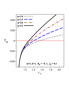
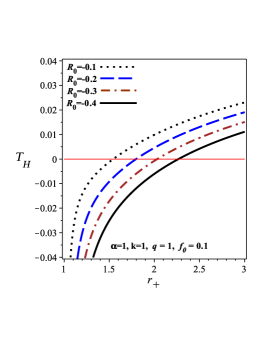
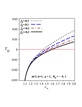
Figure 3: $T_{H}$ versus $r_{+}$ for different values of the parameters.

IV Conclusions

The exact (un)charged accelerating black hole solutions in three-dimensional spacetime were extracted by considering $F(R)$ gravity in the (absence) presence of nonlinear electrodynamics. Our results showed that higher-charged accelerating black holes with massive mass have large roots, provided the maximum mass of these black holes could not be more than a critical value (i.e., $m<m_{critical}$). For $m>m_{critical}$, the black holes had two real roots, which might be related to the event and the cosmological horizons. Moreover, there was the same behavior for parameters of $\theta$ and $\alpha$. In other words, there were two roots for the obtained solutions when $\theta>\theta_{critical}$, and $\alpha>\alpha_{critical}$. The real root of the charged accelerating black holes decreased by increasing the parameter of $F(R)$ gravity ($f_{0}$) and the absolute value of the Ricci scalar $\left|R_{0}\right|$.

Another result was related to the obtained asymptotical behavior of these black holes. It was not precisely asymptotically AdS and depended on different parameters of gravity.

We obtained the temperature of three-dimensional (un)charged accelerating AdS black holes in $F(R)$ gravity. For uncharged cases, the temperature was always positive (negative) when $r_{+}<\frac{1}{\alpha}$ ($r_{+}>\frac{1}{\alpha}$). For charged cases, there was one real root for the temperature, in which the temperature was negative (positive) before (after) this root. Indeed, the small black holes had a negative temperature, but the large black holes were physical objects. We evaluated the effects of various parameters on the temperature of these black holes that were briefly; i) the higher-charged accelerating BTZ black holes had a large area of the positive temperature. ii) the effect of scalar curvature indicated that the positive temperature area of the black hole increases by decreasing the value of $\left|R_{0}\right|$. iii) the effect of $F(R)$ gravity showed that the negative temperature area of the black hole increases by increasing the value of $f_{0}$.

Data Availability Statement

No data associated in the manuscript

References

- (1) W. Kinnersley, and M. Walker, Phys. Rev. D 2 (1970) 1359.
- (2) J. F. Plebanski, and M. Demianski, Annals Phys. 98 (1976) 98.
- (3) J. B. Griffiths, and J. Podolsky, Int. J. Mod. Phys. D 15 (2006) 335.
- (4) M. Appels, R. Gregory, and D. Kubiznak, Phys. Rev. Lett. 117 (2016) 131303.
- (5) M. Astorino, Phys. Rev. D 95 (2017) 064007.
- (6) A. Anabalon, M. Appels, R. Gregory, D. Kubiznak, R. B. Mann, and A. Övgün, Phys. Rev. D 98 (2018) 104038.
- (7) R. Gregory, and A. Scoins, Phys. Lett. B 796 (2019) 191.
- (8) J. Zhang, Y. Li, and H. Yu, JHEP 02 (2019) 144.
- (9) W. Ahmed, H. Z. Chen, E. Gesteau, R. Gregory, and A. Scoins, Class. Quantum Grav. 36 (2019) 214001.
- (10) K. Destounis, R. D. B. Fontana, and F. C. Mena, Phys. Rev. D 102 (2020) 044005.
- (11) A. Ball, Class. Quantum Grav. 38 (2021) 195024.
- (12) S. Jiang, and J. Jiang, Phys. Lett. B 823 (2021) 136731.
- (13) M. Zhang, and J. Jiang, Phys. Rev. D 103 (2021) 025005.
- (14) T. C. Frost, and V. Perlick, Class. Quantum Grav. 38 (2021) 085016.
- (15) B. Eslam Panah, and Kh. Jafarzade, Gen. Relativ. Gravit. 54 (2022) 19.
- (16) J. A. R. Cembranos, L. J. Garay, and S. A. Ortega, Eur. Phys. J. C 82 (2022) 786.
- (17) A. Ashoorioon, M. B. Jahani Poshteh, and R. B. Mann, Phys. Rev. Lett. 129 (2022) 031102.
- (18) M. Born, and L. Infeld, Proc. Roy. Soc. Lond. A 144 (1934) 425.
- (19) H. H. Soleng, Phys. Rev. D 52 (1995) 6178.
- (20) M. Hassaine, and C. Martinez, Phys. Rev. D 75 (2007) 027502.
- (21) S. H. Hendi, JHEP 03 (2012) 065.
- (22) S. I. Kruglov, Annals Phys. 353 (2015) 299.
- (23) S. I. Kruglov, Int. J. Mod. Phys. D 26 (2017) 175007.
- (24) H. Maeda, M. Hassaine, and C. Martinez, Phys. Rev. D 79 (2009) 044012.
- (25) B. Eslam Panah, Europhys. Lett. 134 (2021) 20005.
- (26) S. H. Mazharimousavi, Mod. Phys. Lett. A 37 (2022) 2250170.
- (27) G. W. Gibbons, and C. A. R. Herdeiro, Phys. Rev. D 63 (2001) 064006.
- (28) E. S. Fradkin, and A. A. Tseytlin, Phys. Lett. B 163 (1985) 123.
- (29) D. P. Sorokin, Fortschr. Phys. 70 (2022) 2200092.
- (30) E. Ayon-Beato, and A. Garcia, Phys. Rev. Lett. 80 (1998) 5056.
- (31) E. Ayon-Beato, and A. Garcia, Gen. Relativ. Gravit. 37 (2005) 635.
- (32) I. Dymnikova, Class. Quant. Grav. 21 (2004) 4417.
- (33) S. A. Hayward, Phys. Rev. Lett. 96 (2006) 031103.
- (34) C. Corda, and H. J. Mosquera Cuesta, Mod. Phys. Lett. A 25 (2010) 2423.
- (35) L. Balart, and E. C. Vagenas, Phys. Lett. B 730 (2014) 14.
- (36) R. Garcia-Salcedo and N. Breton, Int. J. Mod. Phys. A 15 (2000) 4341.
- (37) V. A. De Lorenci, R. Klippert, M. Novello, and J. M. Salim, Phys. Rev. D 65 (2002) 063501.
- (38) M. Sami, N. Dadhich, and T. Shiromizu, Phys. Lett. B 568 (2003) 118.
- (39) E. Elizalde, J. E. Lidsey, S. Nojiri, and S. D. Odintsov, Phys. Lett. B 574 (2003) 1.
- (40) M. Novello, S. E. Perez Berglia a, and J. Salim, Phys. Rev. D 69 (2004) 127301.
- (41) A. Karch, and A. O’Bannon, JHEP 09 (2007) 024.
- (42) R. -G. Cai, and Y.-W. Sun, JHEP 09 (2008) 115.
- (43) J. Jing, Q. Pan, and S. Chen, JHEP 11 (2011) 045.
- (44) M. Baggioli, and O. Pujolas, JHEP 12 (2016) 107.
- (45) E. Blauvelt, S. Cremonini, A. Hoover, L. Li, and S. Waskie, Phys. Rev. D 97 (2018) 061901.
- (46) H. A. Gonzalez, M. Hassaine, and C. Martinez, Phys. Rev. D 80 (2009) 104008.
- (47) S. Gunasekaran, R. B. Mann and D. Kubiznak, JHEP 11 (2012) 110.
- (48) J. Diaz-Alonso, and D. Rubiera-Garcia, Gen. Relativ. Gravit. 45 (2013) 1901.
- (49) S. H. Hendi, S. Panahiyan, and R. Mamasani, Gen. Relativ. Gravit. 47 (2015) 91.
- (50) B. Eslam Panah, S. H. Hendi, S. Panahiyan, and M. Hassaine, Phys. Rev. D 98 (2018) 084006.
- (51) S. I. Kruglov, Eur. Phys. J. C 82 (2022) 292.
- (52) G. Arenas-Henriquez, F. Diazb, and Y. Novoa, JHEP 05 (2023) 072.
- (53) S. Capozziello, V. F. Cardone, S. Carloni and A. Troisi, Int. J. Mod. Phys. D 12 (2003) 1969.
- (54) S. M. Carroll, V. Duvvuri, M. Trodden, and M. S. Turner, Phys. Rev. D 70 (2004) 043528.
- (55) T. P. Sotiriou, and V. Faraoni, Rev. Mod. Phys. 82 (2010) 451.
- (56) S. Nojiri, and S. D. Odintsov, Phys. Rept. 505 (2011) 59.
- (57) A. A. Starobinsky, Phys. Lett. B 91 (1980) 99.
- (58) S. Nojiri, S. D. Odintsov, and V. K. Oikonomou, Phys. Rept. 692 (2017) 1.
- (59) S. Capozziello, and A. Troisi, Phys. Rev. D 72 (2005) 044022.
- (60) S. Capozziello, A. Stabile, and A. Troisi, Phys. Rev. D 76 (2007) 104019.
- (61) J. Maldacena, Adv. Theor. Math. Phys. 2 (1998) 231.
- (62) E. Witten, Adv. Theor. Math. Phys. 2 (1998) 253.
- (63) S. S. Gubser, I. R. Klebanov, and A. M. Polyakov, Phys. Lett. B 428 (1998) 105.
- (64) S. W. Hawking, and D. N. Page, Commun. Math. Phys. 87 (1983) 577.
- (65) E. Witten, Adv. Theor. Math. Phys. 2 (1998) 505.
- (66) A. Chamblin, R. Emparan, C. V. Johnson, and R. C. Myers, Phys. Rev. D 60 (1999) 104026.
- (67) M. M. Caldarelli, G. Cognola, and D. Klemm, Class. Quant. Grav. 17 (2000) 399.
- (68) D. F. Jardim, M. E. Rodrigues, and M. J. S. Houndjo, Eur. Phys. J. Plus 127 (2012) 123.
- (69) D. -C. Zou, S. -J. Zhang, and B. Wang, Phys. Rev. D 89 (2014) 044002.
- (70) H. -S. Liu, H. Lu, and C. N. Pope, JHEP 06 (2014) 109.
- (71) S. H. Hendi, B. Eslam Panah, and S. Panahiyan, JHEP 11 (2015) 157.
- (72) J. Zhang, Y. Li, and H. Yu, JHEP 02 (2019) 144.
- (73) W. Cong, D. Kubiznak, and R. B. Mann, Phys. Rev. Lett. 127 (2021) 091301.
- (74) W. Cong, D. Kubiznak, R. Mann, and M. R. Visser, JHEP 08 (2022) 174.
- (75) P. Paul, et al., Nucl. Phys. B 993 (2023) 116259.
- (76) P. Bueno, P. A. Cano, J. Moreno, and G. van der Velde, Phys. Rev. D 107 (2023) 064050.
- (77) J. Barrientos, A. Cisterna, D. Kubiznak, and J. Oliva, Phys. Lett. B 834 (2022) 137447.
- (78) T. Hale, D. Kubiznak, O. Svitek, and T. Tahamtan, [arXiv:2303.16928].
- (79) A. Achucarro, and P. K. Townsend, Phys. Lett. B 180 (1986) 89.
- (80) E. Witten, Nucl. Phys. B 311 (1986) 46.
- (81) M. Zhang, and R. B. Mann, Phys. Rev. D 100 (2019) 084061.
- (82) M. Astorino, JHEP 01 (2011) 114.
- (83) W. Xu, K. Meng, and L. Zhao, Class. Quantum Grav. 29 (2012) 155005.
- (84) W. Xu, K. Meng, and L. Zhao, Commun. Theor. Phys. 58 (2012) 59.
- (85) G. Arenas-Henriquez, R. Gregory, and A. Scoins, JHEP 05 (2022) 063.
- (86) B. Eslam Panah, Fortschr. Phys. 2023 (2023) 2300012.
- (87) R. Emparan, J. F. Pedraza, A. Svesko, M. Tomasevic, and M. R. Visser, JHEP 11 (2022) 073.
- (88) S. H. Hendi, B. Eslam Panah, and R. Saffari, Int. J. Mod. Phys. D 23 (2014) 1450088.
- (89) B. Eslam Panah, Phys. Lett. B 787 (2018) 45.