Ab initio uncertainty quantification in scattering analysis of microscopy

Abstract

Estimating parameters from data is a fundamental problem in physics, customarily done by minimizing a loss function between a model and observed statistics. In scattering-based analysis, it is common to work in the reciprocal space. Researchers often employ their domain expertise to select a specific range of wavevectors for analysis, a choice that can vary depending on the specific case. We introduce another paradigm that defines a probabilistic generative model from the beginning of data processing and propagates the uncertainty for parameter estimation, termed the ab initio uncertainty quantification (AIUQ). As an illustrative example, we demonstrate this approach with differential dynamic microscopy (DDM) that extracts dynamical information through minimizing a loss function for the squared differences of the Fourier-transformed intensities, at a selected range of wavevectors. We first show that DDM is equivalent to fitting a temporal variogram in the reciprocal space using a latent factor model as the generative model. Then we derive the maximum marginal likelihood estimator, which optimally weighs information at all wavevectors, therefore eliminating the need to select the range of wavevectors. Furthermore, we reduce the computational cost of computing the likelihood function by more than a hundred thousand times, without approximation, by utilizing the generalized Schur algorithm for Toeplitz covariances. Simulated studies of a wide range of dynamical systems validate that the AIUQ method substantially improves estimation accuracy and enables model selection with automated analysis. The utility of AIUQ is also demonstrated by three distinct sets of experiments: first in an isotropic Newtonian fluid, pushing limits of optically dense systems compared to multiple particle tracking; next in a system undergoing a sol-gel transition, automating the determination of gelling points and critical exponent; and lastly, in discerning anisotropic diffusive behavior of colloids in a liquid crystal. These outcomes collectively underscore AIUQ’s versatility to capture system dynamics in an efficient and automated manner.

I Introduction

Physical experiments are integral to advancing basic science and technology. However, the cost and efforts to process and analyze data have also increased dramatically, which can sometimes impede progress. There is a pressing need to develop fast and accurate statistical learning algorithms that leverage existing knowledge for data processing to accelerate discovery. One of the core challenges in this context is parameter estimation from data, by minimizing a loss function that quantifies the difference between the modeled and observed statistics. Notably, the estimation can critically depend on the selection of the loss function and statistics to analyze, especially for spatiotemporally correlated measurements. In the scattering analysis of dynamics, for instance, the range of wavevectors in reciprocal space sometimes needs to be chosen in a case-by-case manner, which prohibits its use in high-throughput experiments.

In this work, we introduce another paradigm that defines a probabilistic generative model from the beginning of data processing. Then we propagate the uncertainty throughout the analysis by integrating out the random processing, to derive an optimal statistical estimator, such as the maximum marginal likelihood estimator, implemented in fast algorithms. In scattering analysis, we show that the new estimator automatically weighs information from data at different bases, such as different wavevectors in Fourier-based analysis, and lifts the barriers for selecting wavevectors to fit the loss function.

We apply our automated and scalable analysis to video microscopy, one of the most ubiquitous tools to access the microscopic realm, enabling the observation of microscopic objects such as cells, microcapillaries, bacteria, and colloids. Contemporary video microscopy offers not only visual insight but also versatility and power, supporting multiplexing imaging and capturing time sequences of dynamical processes. Approaches of processing video microscopy can be broadly defined in two classes: particle tracking tools and basis decomposition tools. Particle tracking tools start with separating particle intensity profiles from the background for various techniques including fluorescence microscopy [1], total internal reflection fluorescence microscopy [2], and dark field microscopy [3, 4]. Once the particle profiles have been identified in individual frames, the trajectories of particles between consecutive time frames are linked using multiple particle tracking (MPT) algorithms, such as the Crocker-Grier Algorithm [5], originally written in Interactive Data Language, and was later implemented in MATLAB [6] and in Python [7]. Particle tracking tools, including ImageJ [8] and Trackmate [9], have also been used for analyzing biophysical and cellular processes. Machine learning tools were developed for static cellular images, such as the cell profiling tools (e.g. CellProfiler [10]) and segmentation tools (e.g. CellPose [11]). Although there are well-established frameworks that explain static and dynamic errors, such as those proposed by [12, 13], MPT algorithms in use still depend on several user-specified parameters for localization and selection of search radius for linking particle trajectories. As a result, the quality of particle-based tools can be unsatisfactory due to e.g., non-elliptical objects, optically dense systems, changes in size, shape, and fluorescent intensity.

On the other hand, basis decomposition tools reconstruct microscopy images through basis functions. One of the representative tools is differential dynamic microscopy, which is introduced in [14, 15]. These seminal works innovatively treat each pixel of the image from a microscopy video as probes in dynamic light scattering [16], which can extract dynamical information of the system by correlating photon counts at distinct time points. In DDM, the squared difference of Fourier-transformed intensity at any two time frames is related to the intermediate scattering function [1], which encodes pattern information of dynamic processes. As such, DDM analysis of video microscopy does not require localizing the particles and linking their trajectory. Thus, it is well-suited as a complement to tracking-based tools such as MPT. DDM has been applied to a broad range of soft materials and biological systems, including, for instance, bacteria motility [17, 18], colloidal gels [19], Viscoelastic processes [20], active filament dynamics [21], and protein gelation dynamics [22].

However, there are still several barriers prohibiting DDM from achieving full automation in high-throughput experiments. First and foremost, one needs to select a range of wavevectors to estimate the parameters in the intermediate scattering function, and the results can depend on these choices. Second, due to the lack of a generative model, the uncertainty of the estimation was not quantified, and model selection from data is challenging. Third, though computation of DDM can be accelerated by subsampling [23], and computing the Fourier transformation of the images instead of the image differences [24], a principled way for reducing the storage and accelerating the computation while retaining the most information is needed. These problems are common for other scattering approaches, such as dynamic light scattering [16, 25], thus solving them can advance a wide range of characterization techniques in physical experiments.

Our contributions are three-fold. First of all, we introduce a new generative model of scattering analysis of microscopy in Sec. III.1. We show that conventional estimation of the parameters in DDM is equivalent to fitting a temporal variogram in the Fourier space using the generative model in Sec. III.2. We derive the maximum marginal likelihood estimator (MMLE) after integrating out the latent factor processes introduced in Sec. III.3. As information on each wavevector is weighed appropriately by the likelihood, one can utilize all wavevectors instead of tailoring the range for different systems. Second, directly computing the MMLE is prohibitively slow due to computing inversion and log determinants of a large number of covariance matrices. By evoking the Toeplitz structure of the covariances, we apply the generalized Schur algorithm [26] to accelerate the computation of the marginal likelihood function without approximation in Sec. IV.1, reducing the computational order from cubic to pseudo-linear (or linear with respective to a log multiplicative constant) scaling to the number of time points, without approximating the likelihood. We show in Sec. IV.2 that computational cost can be further reduced with a principled way of data reduction. Taken together, for a typical microscopy video with $500\times 500$ pixels and $500$ time frames, our approach is more than $10^{5}$ times faster than the direct computation of the likelihood function. Third, the generative model and fast algorithm enable a wide range of applications, such as analyzing anisotropic processes, discussed in Sec. III.4. Finally, the new probabilistic approach provides uncertainty quantification of the estimation, and the likelihood can be utilized to select physical models by data. We demonstrate the approach by simulation studies and three distinct types of experiments, including optimally dense particles, high-throughput determinant of gelling point, and estimation anisotropic processes, where data processing and analysis are automated for these applications.

We refer to this approach which provides a probabilistic generative model and propagates the uncertainty from the beginning of the data analysis, the ab initio uncertainty quantification approach. The phrase ab initio used herein should not be confused with the first principles calculation in quantum physics [27], though the philosophy of the computation may share some commonalities. Physical or machine learning approaches that minimize a loss function for parameter estimation can motivate the development of the corresponding generative model, and the generative model enables us to scrutinize the underlying model assumptions made in estimation, and to build a more efficient estimator for different techniques.

II Background for scattering analysis of microscopy

As an example, we first introduce the background and analysis for Differential Dynamic Microscopy (DDM) [14, 15], which converts real-space coordinates into wavevectors in reciprocal space, and computes image correlations akin to Dynamic Light Scattering (DLS), which has led to its characterization as “scattering using microscopy”. Notable advantages of DDM include its compatibility with particles of different shapes [28], fast-moving particles [29], the ability to track particles and fluctuations at high optical density below the diffraction limit [30].

To start, we consider a system of $M$ particles in a 2D space with $\mathbf{x}_{m}(t)=(x_{m,1}(t),x_{m,2}(t))^{T}$ being the 2D particle location of particle $m$ at time $t$, for $m=1,...,M$. The normalized Fourier-transformed intensity can be written as the summation of the particle positions in the reciprocal space

$$\psi(\mathbf{q},t)=\frac{1}{\sqrt{M}}\sum^{M}_{m=1}\exp(-i\mathbf{q}\cdot\mathbf{x}_{m}(t)).$$ (1)

where $i$ denotes the imaginary unit. Assume the particles do not interact with each other [1]. The intermediate scattering function (ISF), an important function encapsulating the time evolution of particle self-correlation, is characterized by a vector of parameters $\bm{\theta}$ below,

$$f_{\bm{\theta}}(\mathbf{q},\Delta t) =\mbox{Cov}(\psi(\mathbf{q},t),\psi^{*}(\mathbf{q},t+\Delta t))$$

$$=\Bigl{<}\frac{1}{M}\sum^{M}_{m=1}\exp\left(i\mathbf{q}\cdot\Delta\mathbf{x}_{m}(t,\Delta t)\right)\Bigr{>},$$ (2)

where $\mbox{Cov}(\cdot,\cdot)$ denotes the covariance operator, $\psi^{*}$ is the complex conjugate of $\psi$, $\Delta\mathbf{x}_{m}(t,\Delta t)=\mathbf{x}_{m}(t+\Delta t)-\mathbf{x}_{m}(t)$, $\mathbf{q}$ is a 2D wavevector and $\langle\cdot\rangle=\mathbb{E}[\cdot]$ is the ensemble or expectation over time $t$. Here we use the notation $\langle\cdot\rangle$ and $\mathbb{E}[\cdot]$ interchangeably, to make it understandable to both physics and statistics communities. The derivation of Eq. (2) is given in Appendix A.

Various processes have a closed-form expression of ISF. A few examples of closed-form ISF are derived in Appendix A and summarized in Table 3. For instance, for Brownian motion (BM) or diffusive processes, the intermediate scattering function is $f_{BM}(\mathbf{q},\Delta t)=\exp(-q^{2}D\Delta t)$, where $q=||\mathbf{q}||$ and here the only parameter of ISF is $\theta=D$, the diffusion coefficient. By the cumulant theorem [31], the ISF can be approximately characterized by the mean squared displacement (MSD), discussed in Appendix A. While it is a more flexible way to estimate ISF, it also requires the estimation of a larger number of parameters.

We denote the light intensity of pixel $\mathbf{x}$ at time $t$ to be $y(\mathbf{x},t)$. In Eq. (2), the ISF is the ensemble average of the 2D spatial Fourier representation of the displacements of the particles from time $t$ to $t+\Delta t$. To relate the ISF to pixel intensity in the Cartesian space, the Fourier-transformed difference in image intensity is studied in DDM [14, 15]: $\Delta{\hat{y}}(\mathbf{q},t,\Delta t)=\mathcal{F}(y(\mathbf{x},t+\Delta t)-y(\mathbf{x},t))$, with $\mathcal{F}(\cdot)$ denoting the 2D discrete Fourier transformation computed by fast Fourier transformation (FFT) [32]. The time ensemble of this quantity, often referred to as the image structure function, $D(\mathbf{q},\Delta t)=\langle\Delta{\hat{y}}(\mathbf{q},t,\Delta t)^{2}\rangle$, is often modeled below:

$$D(\mathbf{q},\Delta t)=A(\mathbf{q})(1-f_{\bm{\theta}}(\mathbf{q},\Delta t))+B,$$ (3)

where $A(\mathbf{q})$ is the real-valued scalar of amplitude parameter for wavevector $\mathbf{q}$, $f_{\bm{\theta}}$ is the ISF defined in Eq. (2), $B$ denotes a random noise with a mean value $\bar{B}$. Then we have $J$ distinct ISF for each $\Delta t$, and $n$ time frames. For an isotropic process in square field of view with $N$ pixels, we denote an index set $\mathcal{S}_{j}=\{(j^{\prime}_{1},j^{\prime}_{2}):q^{2}_{j^{\prime}_{1},1}+q^{2}_{j^{\prime}_{2},2}=q^{2}_{j}\}$ for $j=1,...,J$, which contains the indices of the $j$th ‘ring’ of the Fourier-transformed quantity with amplitude $q_{j}=\frac{2\pi j}{\Delta x_{min}\sqrt{N}}$, with $\Delta x_{min}$ being the pixel size, i.e. the length of a pixel in one coordinate, and $N$ is the number of pixels in one frame. In total, there are J rings of Fourier-transformed intensities. Furthermore, we denote $\mathbf{D}$ as the $J\times(n-1)$ matrix with $(j,k)$th term being the observed image structure function $D(q_{j},\Delta t_{k})=\langle\Delta{\hat{y}}(\mathbf{q}_{\mathbf{j}^{\prime}},t,\Delta t_{k})^{2}\rangle$, where now the ensemble is over both time $t$ and indices within each ring $\mathbf{j}^{\prime}\in\mathcal{S}_{j}$. Let $\mathbf{D}_{m}$ denote the model output of $\mathbf{D}$, where the $(j,k)$th entry of $\mathbf{D}_{m}$ is $D_{m}(q_{j},\Delta t_{k})=A_{j}(1-f_{\bm{\theta}}(q_{j},\Delta t_{k}))+\bar{B}$ with $\bar{B}$ denoting the mean for the random quantity $B$. In DDM, the parameters are often estimated by minimizing a loss function between the observed and modeled image structure functions

$$(\bm{\theta}_{est},\mathbf{A}_{est},\bar{B}_{est})=\underset{\bm{\theta},\mathbf{A}_{1:J},\bar{B}}{\operatorname{argmin}}\mbox{Loss}(\mathbf{D}_{m},\mathbf{D}),$$ (4)

with $\mathbf{A}_{est}=[A_{est,1},...,A_{est,J}]^{T}$ being a J-vector of amplitudes. A typical choice of the loss function is either the $L_{2}$ or $L_{1}$ loss.

As the parameter space has a high dimension, the ISF is often fit separately for each wavevector from a selected range [14, 18, 33, 34], and then estimators at different wavevectors are averaged to obtain $\bm{\theta}$. Some variants of DDM [35, 36, 37] use different pre-specified estimators for $\bar{B}_{est}$ and an unbiased estimator of $A_{est,j}=2\langle\hat{y}(\mathbf{q}_{\mathbf{j}^{\prime}},t)^{2}\rangle_{\mathbf{j}^{\prime}\in\mathcal{S}_{j},t}-\bar{B}_{est}$ to estimate $A_{j}$, leaving $\bm{\theta}$ in the ISF the only parameters to be numerically optimized. A summary of the estimators $\bar{B}_{est}$ is introduced in [23]. In [20, 23], the ISF is approximated by MSD at wavevector, i.e. $f_{\bm{\theta}}(q,\Delta t)\approx\exp\left(-q^{2}\langle\Delta x^{2}(\Delta t)\rangle/4\right)$, and Eq. (3) is directly inverted at each $\Delta t$ to obtain the estimator of MSD $\langle x^{2}(\Delta t)\rangle$. In [38], the MSD is obtained through iterative optimization to reduce numerical instability. Almost all existing approaches seeking to fit image structure function in Eq. (3) rely on selecting a subset of wavevectors to analyze, whereas selecting and reweighing the information at different wavevectors can be hard for a new system. This difficulty arises from the substantial variations in amplitudes $A_{j}$ and the correlation of the image structure function at different lag times. A principled way to properly aggregate the information at different wavevectors can unlock the tremendous potential for DDM to attain complete automation in this process, yet this has not been fully realized so far.

To solve the challenge of optimally weighing information at different wavevector, a key question must be answered: What is the probabilistic model implicitly assumed for the real-space image intensity in DDM? We bridge the physical approach and a probabilistic model to answer this question in Section III.

III Latent factor processes of video microscopy

III.1 A latent factor model of isotropic processes

Let us first focus on isotropic processes, where the ISF is the same at each ring of pixels in the reciprocal space. Extension to anisotropic processes will be discussed in Section III.4. Consider a latent factor model of an $N=N_{1}\times N_{2}$ pixels of real-valued image intensity $\mathbf{y}(t)=[y(\mathbf{x}_{1},t),...,y(\mathbf{x}_{N},t)]^{T}$ at time $t$ below

$$\mathbf{y}(t)=\frac{1}{\sqrt{N}}\mathbf{W}^{*}\mathbf{z}(t)+\bm{\epsilon}(t),$$ (5)

where $\bm{\epsilon}(t)\sim\mathcal{N}(\mathbf{0},\frac{\bar{B}}{2}\mathbf{I}_{N})$ is an N-dimensional Gaussian white noise vector with variance $\frac{\bar{B}}{2}$ and $\mathbf{I}_{N}$ being the identity matrix of N dimensions, the $N\times N$ matrix $\mathbf{W}^{*}$ is a 2D inverse Fourier basis (or complex conjugate of the Fourier basis), which relates the $N$ observation of an image at time $t$ from Cartesian space $\mathbf{x}=(x_{1},x_{2})^{T}$ to a set of random factor processes $\mathbf{z}(t)$ in the reciprocal space $\mathbf{q}=(q_{1},q_{2})^{T}$. The latent factor $\mathbf{z}(t)$ is an $N$ dimensional complex random vector: $\mathbf{z}(t)=\mathbf{z}_{re}(t)+i\mathbf{z}_{im}(t)$, with each random factor at $n$ time points independently following a zero-mean multivariate normal distribution: $\mathbf{z}_{j^{\prime},re}\sim\mathcal{MN}(\mathbf{0},\frac{A_{j}}{4}\mathbf{R}_{j})$ and $\mathbf{z}_{j^{\prime},im}\sim\mathcal{MN}(\mathbf{0},\frac{A_{j}}{4}\mathbf{R}_{j})$ for $j=1,...,J$. The $(k_{1},k_{2})$th entry of $\mathbf{R}_{j}$ is characterized by ISF: $R_{j}(k_{1},k_{2})=f_{\bm{\theta}}(q_{j},\Delta t_{k})$ with $\Delta t_{k}=|k_{2}-k_{1}|\Delta t_{min}$ with $\Delta t_{min}$ being the interval between two consecutive time frames. The key is that the correlation matrix $\mathbf{R}_{j}$ of the latent factor is formed by the ISF from the physical process. This means each entry of the real and imaginary random factors corresponds to one Fourier-transformed quantity, where the covariance is parameterized by the amplitude and intermediate scattering function: $\mathbb{E}[z_{\mathbf{q},re}(t)z_{\mathbf{q},re}(t+\Delta t)]=\mathbb{E}[z_{\mathbf{q},im}(t)z_{\mathbf{q},im}(t+\Delta t)]=\frac{A(\mathbf{q})}{4}f(\mathbf{q},\Delta t)$. Without loss of generality, we assume $N_{1}=N_{2}=\sqrt{N}$, i.e. square image at each time frame.

III.2 DDM is fitting the temporal variogram of the latent factor model in the reciprocal space

Here we draw the connection between DDM in fitting the image structure function and the latent factor model in Eq. (5). Note that the normalized discrete Fourier basis $\mathbf{W}/\sqrt{N}$ is a unitary matrix, i.e. $\mathbf{W}\mathbf{W}^{*}=N\mathbf{I}_{N}$. By multiplying $\mathbf{W}/\sqrt{N}$ on both sides of Eq. (5) and splitting the transformed vector into the real and imaginary parts $\mathbf{\hat{y}}(t)=\frac{\mathbf{W}\mathbf{y}(t)}{\sqrt{N}}=\mathbf{\hat{y}}_{re}(t)+i\mathbf{\hat{y}}_{im}(t)$, we have

$$\mathbf{\hat{y}}_{re}(t)=\mathbf{z}_{re}(t)+\bm{\hat{\epsilon}}_{re}(t),$$ (6)

$$\mathbf{\hat{y}}_{im}(t)=\mathbf{z}_{im}(t)+\bm{\hat{\epsilon}}_{im}(t),$$ (7)

where $\bm{\hat{\epsilon}}_{re}(t)\sim\mathcal{MN}(\mathbf{0},\frac{\bar{B}}{4}\mathbf{I}_{N})$ and $\bm{\hat{\epsilon}}_{im}(t)\sim\mathcal{MN}(\mathbf{0},\frac{\bar{B}}{4}\mathbf{I}_{N})$ are both multivariate normal distribution with a diagonal covariance $\frac{\bar{B}}{4}\mathbf{I}_{N}$; $\mathbf{z}_{re}(t)$ and $\mathbf{z}_{im}(t)$ are both $N$ dimensional random vectors, where each entry corresponds to one wavevector $\mathbf{q}$ in the reciprocal space at time $t$.

We denote ${\hat{y}}_{\mathbf{q}}(t)$ and ${\hat{y}}_{\mathbf{q}}(t+\Delta t)$ to be the Fourier-transformed quantities at time frame $t$ and $t+\Delta t$ respectively, both on the wavevector $\mathbf{q}$. Then, we decompose their difference into the real and imaginary parts: ${\hat{y}}_{\mathbf{q}}(t+\Delta t)-{\hat{y}}_{\mathbf{q}}(t)=\Delta{\hat{y}}_{re,\mathbf{q}}(t,\Delta t)+i\Delta{\hat{y}}_{im,\mathbf{q}}(t,\Delta t)$. Based on the sampling model in Eq. (5), both $\Delta{\hat{y}}_{re,\mathbf{q}}(t,\Delta t)$ and $\Delta{\hat{y}}_{im,\mathbf{q}}(t,\Delta t)$ follow the same normal distribution: $\mathcal{N}\left(0,\frac{A(\mathbf{q})}{2}\left(1-f_{\bm{\theta}}(\mathbf{q},\Delta t)\right)+\frac{\bar{B}}{2}\right)$, as derived in Appendix B. Based on this result, one can compute the expectation of the squared difference of the Fourier-transformed intensity between two frames, at any wavevector $\mathbf{q}$ and time difference $\Delta t$:

$$\operatorname{\mathbb{E}}\left[{({\hat{y}}_{\mathbf{q}}(t+\Delta t)-{\hat{y}}_{\mathbf{q}}(t))({\hat{y}}^{*}_{\mathbf{q}}(t+\Delta t)-{\hat{y}}^{*}_{\mathbf{q}}(t))}\right]$$

$$= A(\mathbf{q})(1-f_{\bm{\theta}}(\mathbf{q},\Delta t))+\bar{B},$$ (8)

which is the mean of the image structure function in Eq. (3), the statistics used for estimating parameters in DDM. Eq. (8) means that if we assume the generative model in Eq. (5), the expected value of the image structure function in Eq. (3) is the expected value of ${({\hat{y}}_{\mathbf{q}}(t+\Delta t)-{\hat{y}}_{\mathbf{q}}(t))({\hat{y}}^{*}_{\mathbf{q}}(t+\Delta t)-{\hat{y}}^{*}_{\mathbf{q}}(t))}$, equivalent to a temporal variagram in the reciprocal space. Fitting spatial variogram in real space was extensively studied in the statistics community [39, 40, 41]. However, it is notoriously hard to fit temporal variogram at each wavevector $\mathbf{q}$ in the reciprocal space and aggregate the estimators in an optimal way, since the variogram is correlated at each lag time and the amplitude parameter is drastically different at distinct $\mathbf{q}$. Thus, directly fitting the temporal variogram in the reciprocal space and aggregating the estimators could lead to unstable estimation. Next, we will introduce the maximum marginal likelihood estimator of the parameters, which provides a natural and optimal way to aggregate the information on each wavevector.

III.3 Maximum marginal likelihood estimator

We denote two $n$-vectors $\mathbf{\hat{y}}_{re,j^{\prime}}=[y_{re,j^{\prime}}(t_{1}),...,y_{re,j^{\prime}}(t_{n})]^{T}$ and $\mathbf{\hat{y}}_{im,j^{\prime}}=[y_{im,j^{\prime}}(t_{1}),...,y_{im,j^{\prime}}(t_{n})]^{T}$ to be the Fourier-transformed quantity at wavevector $j^{\prime}$ over all $n$ time frames. Denote the total observations and latent factors by $\mathbf{Y}$ and $\mathbf{Z}$, respectively. We integrate out the random factors to obtain marginal distribution of observations: $p(\mathbf{Y}\mid\bm{\theta},\bm{A}_{1:J},\bar{B})=\int p(\mathbf{Y}\mid\mathbf{Z},\bm{\theta},\bm{A}_{1:J},\bar{B})p(\mathbf{Z}\mid\bm{\theta},\bm{A}_{1:J},\bar{B})d\mathbf{Z}$. The marginal likelihood of $J$ rings of Fourier-transformed quantity in the reciprocal space follows:

$$\mathcal{L}\left(\bm{\theta},\bm{A}_{1:J},\bar{B}\right)$$

$$= \prod^{J}_{j=1}\prod_{j^{\prime}\in\mathcal{S}_{j}}p_{MN}\left(\mathbf{\hat{y}}_{re,j^{\prime}};\,\mathbf{0},\,\bm{\Sigma}_{j}\right)\times p_{MN}\left(\mathbf{\hat{y}}_{im,j^{\prime}};\,\mathbf{0},\,\bm{\Sigma}_{j}\right),$$ (9)

where $\bm{\Sigma}_{j}=\frac{A_{j}}{4}\mathbf{R}_{j}+\frac{\bar{B}}{4}\mathbf{I}_{n}$. Here $\mathcal{S}_{j}$ denotes the index set of the $j$th ring of isotropic processes, for $j=1,...,J$, and $p_{MN}(\mathbf{s};\bm{\mu},\bm{\Sigma})$ denotes the density of an n-vector multivariate normal distribution at real values $\mathbf{s}$ with mean and covariance being $\bm{\mu}$ and $\bm{\Sigma}$ respectively: $p_{MN}(\mathbf{s};\bm{\mu},\bm{\Sigma})=(2\pi)^{-n/2}|\bm{\Sigma}|^{-1/2}\exp\left\{-\frac{1}{2}(\mathbf{s}-\bm{\mu})^{T}\bm{\Sigma}^{-1}(\mathbf{s}-\bm{\mu})\right\}$. The derivation of Eq. (9) is given in Appendix B.

We denote $S_{j}=\#\mathcal{S}_{j}$, the number of transformed pixels within the index set $\mathcal{S}_{j}$, and let the total number of pixels within $J$ rings be $\tilde{N}=\sum^{J}_{j=1}S_{j}$. Note that we do not include the transformed output outside of the $J$ rings in the likelihood function, consistent with DDM, and hence $\tilde{N}<N$. In principle, one can compute the likelihood of all the quantities inside or outside the $J$ rings. However, as the transformed quantities at large wavevectors become similar to noise, we typically only need to include a small number of wavevectors, which is much smaller than $J$. Based on this feature, we will introduce feasible ways to further reduce the computation and storage cost in Section IV.2.

Here one can maximize the marginal likelihood function in Eq. (9) to estimate parameters $\bm{\theta}$, $\mathbf{A}_{1:J}$ and $\bar{B}$. However, direct maximization can become unstable as $\mathbf{A}_{1:J}$ contains $J$ parameters which can be large. The connection between the latent factor model in Eq. (5) enables us to understand the properties of some estimators of the parameters $A_{1:J}$ and $\bar{B}$. For any $\bar{B}$, an unbiased estimator of the amplitude parameter $A_{j}$ follows

$$A_{est,j}=\frac{2}{S_{j}n}\sum_{j^{\prime}\in\mathcal{S}_{j}}\sum^{n}_{k=1}|\hat{y}_{j^{\prime}}(t_{k})|^{2}-{\bar{B}}$$ (10)

for $j=1,...,J$. In practice, we may take the absolute value of $A_{est,j}$ for some of the large $j$ to keep it nonnegative. Then we estimate the model parameter $\bm{\theta}$ and noise parameter $\bar{B}$ by maximizing the marginal likelihood with the estimated $\mathbf{A}_{est,1:J}$ from Eq. (10)

$$(\bm{\theta}_{est},\bar{B}_{est})=\mbox{argmax}_{\bm{\theta},\bar{B}}\mathcal{L}\left(\bm{\theta},\mathbf{A}_{est,1:J},\bar{B}\right).$$ (11)

This step dramatically reduces the dimension of the parameter space and makes numerical optimization much more stable than optimizing in a large parameter space. We use the low-storage quasi-Newton optimization method [42] for estimation $\bm{\theta}$ and $\bar{B}$ by maximizing the logarithm of the marginal likelihood function $\mbox{log}(\mathcal{L}\left(\bm{\theta},\mathbf{A}_{est,1:J},\bar{B}\right))$ in Eq. (9).

Eq. (5) defines a generative model for the untransformed data from the beginning of the analysis, and the latent factor processes are integrated out to propagate the uncertainty to derive the marginal likelihood in Eq. (9) for parameter estimation. Thus we call the method ab initio uncertainty quantification (AIUQ) for scattering analysis of microscopy. Note here we do not need to compute the difference of image pairs as in the image structure function in Eq. (3); instead, we will introduce the generalized Schur algorithm for accelerating the computation of Toeplitz covariances from the marginal likelihood in Eq. (9) in Section IV.

There are two ingredients of the AIUQ approach for scattering analysis of microscopy. The first key part is to model the untransformed intensity by a probabilistic model, where the temporal correlation of each latent factor process is parameterized by an intermediate scattering function at each wavevector. Equivalently, this is to assume a Bayesian prior encoded physics information of the process. The second key ingredient is to integrate (or marginalize) out random factor processes and estimate the governing physical parameters by an asymptotically optimal estimator–the maximum marginal likelihood estimator. Integrating out random quantities in the model is the foundation of Bayesian analysis, which inherently avoids overfitting the data and provides uncertainty quantification. We refer to [43, 44, 45, 46] for more discussion and applications of the marginal likelihood in machine learning and Bayesian analysis.

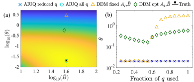
Figure 1: (a) B, D estimates in likelihood space using different methods: AIUQ (x), AIUQ with all q (o), DDM with $A_{j}$, ${\bar{B}}$ ($\triangle$), DDM with optimized $A_{j}$, ${\bar{B}}$ ($\diamond$), whereas the solid dot denotes the truth. The color is the log marginal likelihood by the AIUQ approach with reduced $q$. (b) The D estimate using different methods with the fraction of $q$ used in the estimate.

We illustrate the estimation accuracy of AIUQ using a slow diffusive process in Fig. 1. When dealing with slow dynamics, where the standard deviation of the displacement is smaller than 1/10 of a pixel in each timestep, MPT sometimes fails to accurately capture the underlying dynamics at small lag times, due to the similarity between noise and signal. We compare AIUQ with two DDM approaches. In the first DDM approach, termed DDM with fixed $A_{j}$ and $\bar{B}$, the noise parameter is estimated by $\bar{B}_{est}=D(\mathbf{q}_{min},\Delta t_{min})$, and the amplitude parameter $A_{j}$ is estimated by the unbiased estimator specified in Eq. (10). Then these parameters are substituted into Eq. (4), so that the parameters in ISF are numerically optimized by minimizing the $L_{2}$ loss between the reconstructed and observed image structure functions. In the second DDM approach, termed DDM with optimized $A_{j}$ and $\bar{B}$, parameters are separately estimated for wavevectors by numerically minimizing the $L_{2}$ loss function of the image structure function in Eq. (4). Then the average of the estimation is used to estimate the parameters. AIUQ approaches, with all wavevectors or with a reduced set of wavevectors, use the first $J_{0}$ sets that explain $99\%$ of the variability: $({\sum^{J_{0}}_{j=1}A_{j}})/({\sum^{J}_{j=1}A_{j}})\geq 99\%$, are compared. As demonstrated in Fig. 1(a), AIUQ outperforms other methods in accurately estimating both the noise and diffusion parameters. Fig. 1(b) shows that the estimated parameter is not dependent on $q$ using AIUQ, when a sufficient number of wavevectors is used, as information is naturally weighed by the marginal likelihood in Eq. (9), whereas $q$-dependence is observed in both DDM approaches.

III.4 Extension to anisotropic processes

The analysis of anisotropic fluctuations in the director field was studied using DDM, for estimating directional motions in flow [47] and in response to a magnetic field [48]. To address angle-specific or anisotropic motion, previous works often select a limited angle range centered around the desired direction. For instance, in [28], a specific range of $q$ values is averaged to extract distinct translational Brownian diffusion along perpendicular axes of ellipsoids. Another example is liquid crystal, explored in [49], where a bowtie-shaped $q$-space region along both parallel and perpendicular directions to the director is averaged to extract viscoelastic properties and isolate polarized light contribution. However, constraining $q$ in a certain angle range could discard useful information on other wavevectors outside this range.

The AIUQ approach of scattering analysis of microscopy can be extended to anisotropic processes. Let us consider a 2D anisotropic process, we can split the intermediate function to two coordinates: $f_{\bm{\theta}}(\mathbf{q},\Delta t)=f_{\bm{\theta}_{1}}(q_{1},\Delta t)f_{\bm{\theta}_{2}}(q_{2},\Delta t)$, where $f_{\bm{\theta}_{l}}(q_{l},\Delta t)$ is an intermediate scattering function for the $l$th coordinate, and the parameters can be split to $\bm{\theta}=\{\bm{\theta}_{1},\bm{\theta}_{2}\}$ with $\bm{\theta}_{1}$ and $\bm{\theta}_{2}$ being the parameters of $f_{\bm{\theta}_{l}}(q_{l},\Delta t)$ for $l=1,2$. From the cumulant approximation discussed in Appendix A, one derives the anisotropic ISF

$$f_{\bm{\theta}}(\mathbf{q},\Delta t)\approx\exp\left(-\frac{q^{2}_{1}\langle\Delta x^{2}_{1}(\Delta t)\rangle+q^{2}_{2}\langle\Delta x^{2}_{2}(\Delta t)\rangle}{2}\right),$$

where $\langle\Delta x^{2}_{1}(\Delta t)\rangle$ and $\langle\Delta x^{2}_{2}(\Delta t)\rangle$ are MSD at $\Delta t$ along the two coordinates, respectively. As the process is anisotropic, the ISF is different for each wavevector in general. Then one can compute the maximum marginal likelihood estimator in Eq. (11) with the anisotropic ISF. Since the amplitude $A_{j}$ depends on the transformed intensity at zero lag time and image noise [15, 50]. Thus, $A_{j}$ can be calculated similarly regardless of isotropic or anisotropic processes. The projected intensity on all wavevector can be used in an AIUQ approach, which makes the analysis more stable and accurate.

IV Fast estimation, uncertainty assessment and model selection

IV.1 The generalized Schur method of accelerating computation for Toeplitz covariances

Directly computing the marginal likelihood in Eq. (9) is slow as computing each of $n$-vector multivariate normal requires $\mathcal{O}(n^{3})$ computational operations, from computing the matrix inversion and determinant of the covariance matrix. Assuming we have $J$ rings of Fourier-transformed intensity, and the number of indices in each ring is $S_{j}$, the total computational operations scales as $\mathcal{O}(Jn^{3})+\mathcal{O}(\tilde{N}n^{2})$ operations for isotropic processes, and $\mathcal{O}(\tilde{N}n^{3})$ for anisotropic processes. As the likelihood function needs to be computed tens of times for numerically optimizing the parameters, the computational operations can be up to $10^{15}$ for a regular video with $500\times 500$ pixels and $500$ time frames, which is too computationally expensive. Here we introduce a fast approach that can substantially reduce the computational cost without any approximation to the likelihood function.

Note that as video microscopy is often taken equally spaced in time, which means the covariance matrix $\bm{\Sigma}_{j}$ is a Toeplitz matrix [51] for each j, parameterized by the ISF:

$${\bm{\Sigma}}_{j}=\begin{bmatrix}\tilde{f}_{j,0}&\tilde{f}_{j,1}&\tilde{f}_{j,2}&\dots&\tilde{f}_{j,n-1}\\ \tilde{f}_{j,1}&\ddots&\tilde{f}_{j,1}&\dots&\tilde{f}_{j,n-2}\\ \tilde{f}_{j,2}&\tilde{f}_{j,1}&\ddots&\ddots&\vdots\\ \vdots&\vdots&\ddots&\ddots&\tilde{f}_{j,1}\\ \tilde{f}_{j,n-1}&\tilde{f}_{j,n-2}&\dots&\tilde{f}_{j,1}&\tilde{f}_{j,0}\\ \end{bmatrix},$$ (12)

where $\tilde{f}_{j,k}=\frac{A_{j}}{4}f_{j,k}+\frac{\bar{B}}{4}1_{k=0}$ with $f_{j,k}=f_{\bm{\theta}}(q_{j},\Delta t_{k})$ being the intermediate scattering function at ring $j$ and $\Delta t_{k}$, and $1_{k=0}$ being a Delta function at $k=0$. Consequently, the covariance matrix $\bm{\Sigma}_{j}$ is a Toeplitz matrix. The generalized Schur algorithm was developed in [26, 52] for accelerating the computation, which reduces computing the inversion and log determinant of Toeplitz covariance from $\mathcal{O}(n^{3})$ to $\mathcal{O}(n(\log(n))^{2})$ operations for an $n\times n$ Toeplitz covariance matrix. Thus for computing the marginal likelihood function in Eq. (9), one only needs $\mathcal{O}(Jn(\log(n))^{2})+\mathcal{O}(\tilde{N}n\log(n))$ operations for isotropic processes, where the first term is from computing determinant and matrix inversion of $J$ Toeplitz covariances, and the second term is from computing the $\tilde{N}$ Toeplitz matrix-vector multiplication, through FFT. For anisotropic processes, one only needs $\mathcal{O}(\tilde{N}n(\log(n))^{2})$ operations for computing the likelihood. The generalized Schur method of computing inversion, log determinant, and matrix-vector multiplication for Toeplitz matrices was implemented in the ‘SuperGauss’ algorithm in R platform [53, 54]. The generalized Schur algorithm is a ‘superfast’ algorithm as its complexity is pseudo-linear to the number of observations for decomposing a Toeplitz covariance [52], and other algorithms, such as the Levinson-Durbin algorithm [55] that take $\mathcal{O}(n^{2})$ operations for decomposing a Toeplitz covariance, are generally called fast algorithms. Details of the generalized Schur algorithm are summarized in Appendix C.

IV.2 Data reduction

As the marginal likelihood function in Eq. (9) often needs to be computed tens of times to iteratively find the maximum value, it is of interest to further reduce the computational complexity for large videos in addition to using the generalized Schur algorithm.

For processes with an increased MSD with respect to the increase of lag time, such as subdiffusion or superdiffusion, the transformed intensity rapidly decorrelates at large wavevectors, making it indistinguishable from noise. A typical way for dimension reduction is to choose the first $J_{0}$ rings of Fourier-transformed intensity that explains the most variability of the data: $({\sum^{J_{0}}_{j=1}A_{j}})/({\sum^{J}_{j=1}A_{j}})\geq 1-\varepsilon$, where $\varepsilon$ is a small number, similar to the probabilistic principal component analysis [56]. For instance, choosing $\varepsilon=0.001$ means we have $99.9\%$ of the variability from the transformed intensity explained. As $A_{j}$ becomes close to $0$ at large $j$ and the ‘ring’ gets larger for large $j$, such a choice can substantially reduce the storage and computational requirements by avoiding computing a large number of transformed intensities at high frequency wavevectors. Another way is to ensure that we select a relatively large proportion ($J_{0}/J\geq\beta$) to retain enough information from the signal. For some confined processes, such as the Ornstein–Uhlenbeck (OU) process, where the MSD approaches a plateau at large lag time, using a large fraction of wavevectors is a safer choice, as the temporal correlation of transformed intensities does not decrease at large wavevectors. Having a more conservative threshold that selects a larger $J_{0}$, e.g. $\varepsilon=0.001$ and $\beta=0.5$, is also better for estimating the noise parameter. Here, we emphasize that the selection of $J_{0}$ is mainly for further reducing the storage and computational cost, which is different from selecting the range of wavevectors to analyze in minimizing the loss function in Eq. (4) in DDM.

IV.3 Confidence interval

The uncertainty of parameter estimation can be quantified with the availability of the probabilistic generative model in Eq. (5). Here, estimation errors stem from two aspects: discretization of pixels and parameter estimation. First, the dynamical processes are continuous, whereas analysis is performed on discretized pixels. The pixel-related uncertainty can be big when we have a small number of pixels, and the error becomes small when we have a finer pixel size. Second, similar to all statistical inferences, the stochastic nature of observations introduces uncertainty in parameter estimation. Given a generative model, the uncertainty from statistical analysis can be assessed by either the Frequentist or Bayesian analysis. When distributions of the pivotal quantities have no closed-form expressions, the confidence interval from Frequentist analysis is often approximated by the central limit theorem [57] or bootstrap [58]. The posterior credible interval from Bayesian analysis is by specifying the prior of the parameters and then computing the posterior distribution, often evaluated by the Markov chain Monte Carlo algorithm [59], such as Gibbs sampling and Metropolis algorithm [60, 61]. The parameter uncertainty of Bayesian and Frequentist analysis typically agrees when the sample size approaches infinity.

We quantify both the pixel and estimation uncertainty to construct the confidence interval with the scalable algorithm by the generalized Schur method. To integrate the pixel uncertainty, we compute the maximum marginal likelihood estimator of $(\bm{\theta},\bar{B})$ by letting the associated amplitude of the wavevector $q_{j}$ to be $q_{j}-\Delta q_{min}$ and $q_{j}-\Delta q_{max}$ for $j=1,...,J$ separately. Then we follow [57] to approximate the parameter estimation uncertainty through an asymptotically normal distribution. Notably, the scattering information comes from $M$ trajectories ($M\approx$ 50-200) of individual particles instead of $\sum^{J_{0}}_{j=1}S_{j}$ Fourier-transformed time series, and typically $M\ll N$ ($N\approx 2.5\times 10^{5}$). Thus one may need to discount the likelihood by a power of $M/N$ when computing the uncertainty in asymptotic normality approximation. We integrate both sources of uncertainty to construct the confidence interval of estimated parameters. As will be shown in the simulated studies, the $95\%$ confidence intervals are narrow when the size of the image is not too small, and they cover the truth most of the time.

IV.4 Model selection and diagnostics

Given a few plausible models of ISF, how do we know which one shall be used? Statistical information criteria, such as Akaike information criterion (AIC) [62], may be computed: $\mbox{AIC}=2p-\mbox{ln}(\mathcal{L}(\bm{\theta}_{est},\mathbf{A}_{1:J,est},\bar{B}_{est}))$, where $\mathcal{L}(\bm{\theta}_{est},\mathbf{A}_{1:J,est},\bar{B}_{est})$ denotes the maximum likelihood value and $p$ is the number of parameters. AIC quantifies the predictive error, and hence one selects a model with a small AIC. In practice, models with a larger set of parameters are often selected by AIC, when the number of observations is large. One may compensate by using Bayesian information criterion (BIC) [63], which also penalizes for the number of observations.

Processes,	Small video				Regular video
true parameters	DDM	DDM	AIUQ	AIUQ	DDM	DDM	AIUQ	AIUQ
	fixed	opt	reduced q	all q	fixed	opt	reduced q	all q
BM, $\sigma^{2}_{BM}=.020$	8.3	.36	.020 (.017,.024]	.020 (.017,.024]	2.8	.56	.019 [.019,.020]	.020 [.019,.020]
BM, $\sigma^{2}_{BM}=2.0$	3.8	1.7	2.0 [1.8, 2.4]	2.1 [1.8, 2.4]	3.6	2.8	2.0 [2.0, 2.1]	2.0 [2.0, 2.1]
FBM, $\sigma^{2}_{FBM}=8.0$	7.5	4.2	8.0 (7,10]	8.0 (7,10]	6.7	3.8	8.1 [7.8,8.5)	8.1 [7.8,8.5)
$\alpha=.60$	.75	1.0	.59 [.35,.67)	.59 [.35,.67)	.87	.88	.59 [.58,.61)	.59 [.58,.61)
FBM, $\sigma^{2}_{FBM}=.50$	2.3	.49	.52 (.42,.52]	.52 (.41,.52]	3.0	.74	.50 [.47,.54]	.50 [.46,.55]
$\alpha=1.4$	1.3	1.3	1.4 [1.4,1.5]	1.4[1.4,1.6]	1.3	1.0	1.4 [1.4,1.4]	1.4 [1.3,1.4]
OU, $\sigma^{2}_{OU}=64$	$5.7\times 10^{5}$	3.1	61 (24,191]	61 (13,353]	$7.0\times 10^{4}$	22	61 (44,86)	61 [35,110)
$\rho=.95$	.64	.52	.95 [.89,.98)	.95 [.82,.99)	.71	.57	.95 (.93,.96]	.95 (.91,.97)
OU$+$FBM, $\sigma^{2}_{1}=2.0$	2.2	1.5	1.8 [1.0,3.2]	1.8 [.75.4.4]	1.9	2.5	2.0 (1.6,2.4)	2.0 (1.4,2.7)
$\alpha=.45$	1.3	1.1	.41 [.31,.55)	.40 (.24,.68)	1.2	.76	.44 (.41,.48]	.44 (.38,.51)
$\sigma^{2}_{2}=9.0$	5.6	3.2	9.8 [4.0,28]	9.9 (2.1,54)	7.6	2.1	9.7 (7.1,13]	9.7(5.4,17]
$\rho=.85$	.55	.43	.85 (.74,.93)	.85 (.61,.96)	.62	.50	.85 (.81,.89)	.85 (.77,.91]

Table 1: Parameter estimation for the average absolute deviation of the MSD estimates using different methods. The one closest to the truth is highlighted in bold. Regular videos have 500 $\times$ 500 $\times$ 500, while small videos have size 100 $\times$ 100 $\times$ 100. The brackets give $95\%$ confidence intervals by AIUQ approaches and different types of brackets are due to rounding error. All intervals by AIUQ approaches cover the true parameters given in the first column.

Other than the information criteria, we may also directly compute the one-step predictive error for model selection. To do so, we first divide the microscopy video into two groups, and the first $n_{0}$ time frames are used for estimating parameters. Then we make predictions sequentially on each $n^{*}=n_{0}+1,...,n$ using the one-step-ahead prediction

$$\mathbf{y}_{pred}(t_{n^{*}})=\mathbf{W}^{*}\mathbf{z}_{pred}(t_{n^{*}}),$$ (13)

where for isotropic processes, the $j^{\prime}\in S_{j}$ column of $\mathbf{z}_{pred}(t_{n^{*}})$ is $z_{pred,j^{\prime}}(t_{n^{*}})=A_{est,j}\mathbf{r}^{T}_{est}(t_{n^{*}})(A_{est,j}\mathbf{R}_{est,j}+\bar{B}_{est,j})^{-1}(\hat{\mathbf{y}}_{re,j^{\prime}}(\mathbf{t}_{1:(n^{*}-1)})+i\hat{\mathbf{y}}_{im,j^{\prime}}(\mathbf{t}_{1:(n^{*}-1)}))$ with $\mathbf{r}_{est}(t_{n^{*}})=(f_{\bm{\theta}_{est}}(q_{j},t_{n^{*}}-t_{1}),...,f_{\bm{\theta}_{est}}(q_{j},t_{n^{*}}-t_{n^{*}-1}))^{T}$ is an $n^{*}-1$ vector of ISF, and $\mathbf{R}_{est,j}$ being a $({n^{*}}-1)\times({n^{*}}-1)$ matrix, the $(k,k^{\prime})$th entry of which is $f_{\bm{\theta}_{est}}(q_{j},t_{k}-t_{k^{\prime}})$. On the other hand, the $j$th column of the predictive mean for anisotropic processes follows $z_{pred,j}(t)=A_{est,j}\mathbf{r}^{T}_{est}(t_{n^{*}})(A_{est,j}\mathbf{R}_{est,j}+\bar{B}_{est,j})^{-1}(\hat{\mathbf{y}}_{re,j}(\mathbf{t}_{1:(n^{*}-1)})+i\hat{\mathbf{y}}_{im,j}(\mathbf{t}_{1:(n^{*}-1)}))$, as the ISF is different for each wavevector in general. The generalized Schur algorithm is used for accelerating the computation of predictive mean in Eq. (13) to avoid the direct inversion of the covariance matrices. Then we select the model that minimizes the predictive loss, such as the average root mean squared error. When predictive errors are similar, a model with a smaller number of parameters is preferred.

V Simulated studies

V.1 Isotropic processes

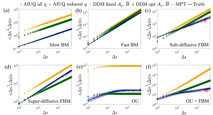
Figure 2: Analyzing simulated studies using different methods,(c) The mean-squared displacements versus lag time from the trajectories of $M$ = 50 simulated particles are analyzed using AIUQ (blue crosses), AIUQ all q (cyan crosses), DDM with fixed $A_{j}$, ${\bar{B}}$ (purple diamonds) and DDM with optimized $A_{j}$, ${\bar{B}}$ (yellow triangle). The analysis is for (a) Slow Brownian Motion, (b) Fast Brownian Motion, (c) Fractional Brownian motion with subdiffusive dynamics, (d) Fractional Brownian motion with superdiffusive motion, (e) Ornstein–Uhlenbeck process and (f) Noisy continuous time random walk. The solid lines denote the truth. The shaded area denotes the 95% interval for AIUQ. The truth overlaps with both AIUQ approaches.

We first compare the estimation accuracy of ISF for isotropic processes through simulations. We simulated videos from six different processes: Brownian motion (BM) with two diffusion coefficients, fractional Brownian motion (FBM) with two power parameters corresponding to subdiffusive and superdiffusive processes, respectively, Ornstein–Uhlenbeck (OU) processes, and a mixture of the OU process and FBM (OU$+$FBM). The ISFs of these processes are provided in Table 3 in Appendix A. For each process, we test the performance of each approach using both a small-sized video with $100\times 100$ pixels and $100$ time frames, and a regular-sized video with $500\times 500$ and $500$ time frames. The algorithms are applicable to videos with different spatial and temporal lengths. The smaller videos contain fewer frames but retain the same timestep, particle size, and essentially the same dynamics.

We compare the AIUQ approaches with a reduced number of wavevectors, and with all wavevectors, two DDM approaches, and MPT. The first AIUQ approach uses the first $J_{0}$ sets (or rings) of wavevectors such that $\sum^{J_{0}}_{j=1}A_{j}/\sum^{J}_{j=1}A_{j}\geq 1-\varepsilon$ and $J_{0}/J>\beta$ with $\varepsilon=0.001$ and $\beta=0.5$, which leads to at least first $50\%$ of rings of wavevectors being selected. The same choice is applied to all simulations discussed in Sec. V.1-V.3. We found that using a less conservative threshold $\varepsilon=0.01$ and $\beta=0$ leads to around the first $25\%$ of sets of wavevector being selected, and producing almost the same estimation for parameters in the intermediate scattering function, but the estimation of the noise parameter may not as good for small videos. The second AIUQ approach uses all $J$ wavevectors, which is computationally slower than the first AIUQ approach. The two routinely used DDM approaches have been described in Sec. III.3. Finally, in MPT, we input the known particle radius which enables the algorithm to effectively choose the optimal band-pass filter, whereas other parameters such as search radius and brightness of the center pixel need to be tuned depending on the specific case.

In Table 1, the true parameters, the estimated parameters by two DDM approaches, AIUQ with reduced and all wavevectors are provided. The AIUQ approaches yield accurate estimations for regular videos, outperforming the two DDM approaches. AIUQ also yields excellent results even when applied to significantly smaller images. Despite a 125$\times$ reduction in image size, the method yields estimations with almost indiscernible error. Furthermore, the $95\%$ confidence intervals of each parameter are given in the brackets, which cover the true parameters. The significant improvement of the performance by the AIUQ approaches is attributed to it appropriately weighing information from each wavevector by the marginal likelihood function in Eq. (9). Consequently, there is no need to choose a specific range of wavevectors for estimation, other than for the purposes of reducing the computational cost. In contrast, the DDM methods require selection and additional weighing of information from different wavevectors, which is typically carried out on a case-by-case basis. Avoiding selecting the range of wavevector can automate the scattering analysis of video microscopy, a key feature for such analysis to be seamlessly integrated into any high-throughput experiments.

The true MSD, estimated MSD by MPT, two DDM and AIUQ approaches of six simulated processes with a regular video size are plotted in Fig. 2. Estimation from the two AIUQ approaches and the true MSD curves overlap for all cases, indicating precise estimation of MSD by the AIUQ approaches. Furthermore, the $95\%$ confidence interval by AIUQ (shown as the blue shaded area) is relatively short, in particular for the two BMs, but they cover most of the underlying truth of MSD. Lastly, MPT is reasonably accurate for most scenarios with case-specific tuning parameters. However, it has a noticeable discrepancy at small $\Delta t$ for BM with slower dynamics (Fig. 2(a)), and at large $\Delta t$ for almost all processes, whereas AIUQ approaches do not have this problem. Furthermore, we record the root mean squared error (RMSE) between the true MSD and estimated MSD by different approaches in Table 4 in Appendix D, and the AIUQ approaches have the smallest estimation error than other approaches in all scenarios, and in particular, the RMSE by two AIUQ approaches are both 5-10 times smaller than the ones by MPT. This means that if the model is properly selected, the AIUQ approach can be more accurate than MPT in terms of estimating the MSD, and they do not require tuning parameters.

The small estimation error by the scattering analysis of microscopy video for the wide range of simulated processes has not been seen before, which is achieved without the need to select wavevectors or tune any parameters. The new approach allows for a smaller image sequence with a shorter time interval to be employed, leading to savings in both time and storage, and yields more accurate estimation when videos with a regular size are used.

V.2 Model selection

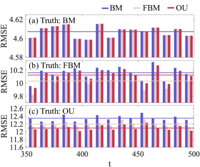
Figure 3: Predictive accuracy as demonstrated by the Root Mean Square Error (RMSE) for (a) Brownian Motion ($\sigma^{2}_{BM}=0.02$) (b) Fractional Brownian Motion ($\sigma^{2}_{FBM}=8$, $\alpha=0.6$) and (c) Ornstein–Uhlenbeck process ($\sigma^{2}{OU}=64$, $\rho=0.5$) trained on the first 300 lag times. The horizontal lines are the average of the RMSEs of each method.

Conventionally, physical models of intermediate scattering function are selected based on pre-existing knowledge of the dynamical process. Here we introduce two ways for model selection among a few candidate choices for microscopy video from data because of the availability of the probabilistic generative model in Eq. (5).

We first show the model selection approach by minimizing the predictive error introduced in Sec. IV.4. We simulate microscopy video of BM, FBM, and OU processes with the regular size (500 $\times$ 500 $\times$ 500). Then we fit three candidate models of ISF for each video using first the $70\%$ of the time frames, and save the other $30\%$ of the time frames for computing one-step ahead root means squared errors (RMSEs) for each time frame, and the average of the RMSEs: $\mbox{AvgRMSE}=\frac{1}{(n-n_{0})}\sum^{n}_{t=n_{0}+1}\left(\frac{1}{N}\sum^{N}_{j=1}(y_{j}(t)-y_{pred,j}(t))^{2}\right)^{\frac{1}{2}}$, where $y_{pred,j}$ is the prediction at the $j$th pixel from Eq. (13), where $n_{0}=350$ is the number of time frames for training the model.

The predictive RMSEs of three models on held-out time frames are plotted as histograms for simulated BM, FBM, and OU processes in Fig. 3 (a)-(c), where each histogram of RMSE is averaged over 10 time frames. The overall AvgRMSEs are shown as the horizontal lines. First, when the underlying process is BM (Fig 3 (a)), three models have almost the same RMSE at all different frames. This is because BM is a special case of FBM with $\alpha=1$. The estimated power parameter yields $\alpha_{est}\approx 0.97$, meaning the FBM model approximately reduces to the BM model in this case. For the OU process, based on binomial approximation, one has $\sigma^{2}_{OU}(1-\rho^{\Delta t})\approx\sigma^{2}_{OU}(1-\rho)\Delta t$, when $1-\rho$ is close to zero. Thus the MSD of OU can also approximate BM relatively well when $\sigma^{2}_{OU}(1-\rho)\approx\sigma^{2}_{BM}$. Indeed, we found $\sigma^{2}_{est,OU}(1-\rho_{est})\approx 0.0196$, a value close to the true sampling model from BM with the parameter $\sigma^{2}_{BM}=0.020$. When the predictive error of these three models is similar, the preferred model is BM due to its simplicity, as it contains fewer fitting parameters in its ISF. Second, when the true process is FBM (Fig 3 (b)), the fitted FBM model consistently yields a smaller predictive RMSE compared to the other two models across most held-out time frames. The AvgRMSE indicated by the pink solid line for FBM remains identifiably lower than the other misspecified models. Third, when the true process is OU (Fig 3 (c)), the AvgRMSE of fitted OU, plotted as the red solid line, is the smallest among the three models. Thus, based on the model selection criteria, we correctly select the true sampling models for all three cases.

Performing model selection with one-step-ahead predictive error requires sequentially predicting intensities on $n-n_{0}$ time frames, which is time-consuming. Instead, we can compute AIC based on the maximum marginal likelihood value. A model with a smaller AIC is preferred as it indicates a smaller prediction error. In Table 2, we show AIC by different models in each column. We notice that the AIC of the three models is almost identical when the underlying dynamics follow a BM, as FBM and OU approximate BM with the estimated parameter. The BM is preferred when AIC is similar, as it has a smaller number of parameters. Similar to the findings in Fig. 3, we found that the correct model has the smallest AIC, corresponding to the best fit, for FBM and OU. Hence, all true models are correctly selected by these two model selection criteria.

simulation/fitting	BM	FBM	OU
BM	2.2320	2.2320	2.2320
FBM	2.6195	2.6173	2.6189
OU	2.6464	2.6455	2.6445

Table 2: AIC of the fitted model is shown in each column. Each row gives one simulation. The smaller the number indicates a better fit and the smallest value in each row is highlighted in bold. The values are multiplied by $10^{8}$.

V.3 Anisotropic processes

Here we test the performance of AIUQ approaches for anisotropic processes. We simulate small and regular-sized videos for anisotropic processes from one BM, and two FBMs with different parameter sets for motions along each coordinate. The parameters used for simulating these three anisotropic processes are plotted by the color bars in Fig. 4. For BM, the variance of the displacement in the $x$ direction of the process is 4 times as large as the one in the y direction. For the first FBM, the motion in the $x$ direction has a larger variance parameter, but the power parameter is smaller than that in the y direction. For the second FBM, both the variance and power parameters of the motion in the $x$ direction are smaller than the ones in $y$ direction.

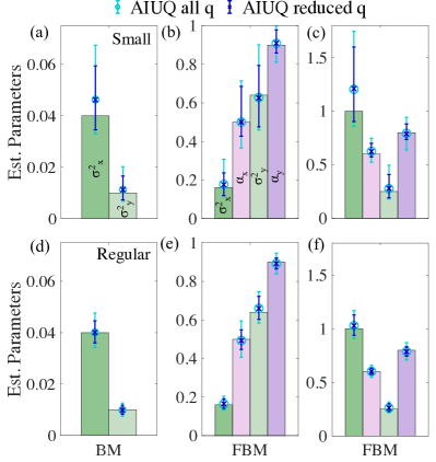
Figure 4: Parameter estimation for anisotropic processes as shown in bar graphs. The top row shows small videos (100 $\times$ 100 $\times$ 100), and the bottom row shows regular videos (500 $\times$ 500 $\times$ 500). (a)(d) Shows the analysis of particles diffusing with two distinct diffusion coefficients along x and y, whereas (b)(c)(e)(f) show fractional Brownian motion with distinct coefficients and exponents.

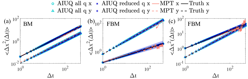
Figure 5: Analyzing simulated studies with anisotropic dynamics. The mean-squared displacements versus lag time from the trajectories of $M$ = 50 simulated particles are analyzed using AIUQ (blue crosses), AIUQ all q (cyan circles and triangles), MPT (pink solid lines). The analysis is for (a) Brownian Motion, (b)(c) Fractional Brownian motion. The shaded area represents the 95% interval of AIUQ reduced q. The truth overlaps with both AIUQ approaches.

In Fig. 4, we plot the estimated parameters and the $95\%$ confidence interval by two AIUQ approaches for small or regular-sized videos of anisotropic processes. The estimated parameters are reasonably accurate even for most of the small videos, and the estimation error is indiscernible for videos with a regular size. Furthermore, the small $95\%$ confidence interval covers all the truth parameters and the interval becomes narrower when the size of the video enlarges. The lengths of the interval quantify whether the precision of the estimation is satisfied, allowing one to strike a balance between the size of the microscopy video and the precision of the analysis.

We plot estimated MSD from the AIUQ and MPT in Fig. 5. In panel (a), our approach correctly identifies that the diffusion coefficient along x is 4 times as large as that along y. Panel (b) shows a subdiffusive case, where the motion along y has both a higher exponent and prefactor, causing the difference of MSD along x and y to grow with lag time. Panel (c) shows another subdiffusive scenario along both axes, where the motion along $y$ has a smaller prefactor yet a larger exponent, causing the MSD along y to grow faster and eventually approach that along x. The estimated MSDs are shown for two AIUQ approaches and MPT. Across all cases, AIUQ accurately replicates MSDs of the simulated dynamics, even when the MSDs in both directions approach one another in the third scenario. Routinely used MPT algorithms [5] typically link particles between two time frames within a pre-specified radius, which may not be optimal for anisotropic processes. Indeed, we found that identifying a suitable set of tuning parameters for MPT is harder for anisotropic processes. In comparison, one does not need to tune parameters in AIUQ approaches, and the estimated MSD from AIUQ all overlap with the truth shown in Fig. 5. Furthermore, for Fig. 5(a)-(b), MPT has a noticeable discrepancy in estimating the MSD at small $\Delta t$ due to the difficulty in separating small signal from noise, whereas AIUQ approaches are accurate. For all processes, the RMSE of estimating MSD by the AIUQ approaches is a few times smaller than the ones by MPT shown in Table 5 in Appendix D.

Furthermore, the $95\%$ confidence interval of the MSD by the AIUQ is small but covers most of the data, indicating that the uncertainty of the estimation is properly quantified. The uncertainty assessments that can cover most of the data with a short interval have not been found in other approaches. Yet it is achievable with the use of a probabilistic generative model and estimation with uncertainty propagated from the beginning of the analysis, or i.e. in an ab initio manner.

DDM approaches were used for analyzing the anisotropic processes [49, 48, 47], but they only use a fraction of the transformed data along the x and y coordinates, selected by researchers. Here, we utilize information from all wavevectors, yielding better accuracy in estimation and enabling appropriate uncertainty assessment without the need for selecting and additional weighing of the information from different wavevectors.

We expect that this algorithm will have broader applicability to analyzing a plethora of biological scenarios involving collective cell motion under various conditions such as chemotaxis [64], durotaxis [65], and haptotaxis [66], especially for dense settings, typically seen in a confluent cell monolayer. In Sec. VI.4, for instance, we will introduce the feasibility of analyzing the anisotropic motion for probes embedded in a lyotropic liquid crystal.

VI Real experimental analysis

VI.1 Materials and Methods

Polyvinyl alcohol (PVA, Mw 85,000-124,000, 87-89% hydrolyzed), dimethylsulfoxide (DMSO), Triton X-100, and disodium cromoglycate (DSCG) salt were purchased from Sigma-Aldrich, and used without further purification. The solutions were weighed and dispersed in ultra-pure water (18.2 M$\Omega$-cm). 4-arm PEG polymers, terminated with primary amide (NH2) and succinimidyl glutarate (SG) groups were purchased from JenKem Technology USA.

Probes (FluoSpheres, yellow-green, carboxylate-modified microspheres) of different sizes ($2r_{p}$ = 100 nm, 200 nm, and 1 $\mu$m) were purchased from Thermo Fisher. All samples were prepared by filling a square capillary (0.10 mm x 1.0 mm x 0.09 mm, Friedrich & Dimmock Inc.), sealing on two ends, and securing onto a glass slide with UV curable glue (Norland Optical Adhesive), to minimize convection due to leaking and evaporation.

The sample is imaged using a Zeiss Axio Observer 7 microscope in fluorescence mode using a Colibri 7 light source, and standard GFP filter sets. The images are captured with a 20x objective, with a numerical aperture of 0.8. A typical image size is 512 x 512 pixels with a pixel size of 0.29 $\mu$m/pixel and T = 500 time steps with a step size of 0.0309 seconds.

VI.2 Diffusive motion with different particle size and number density

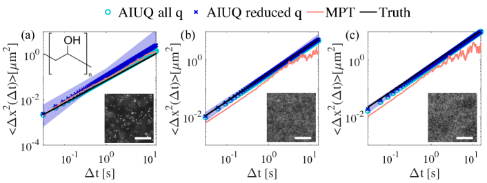
Figure 6: The diagram shows the mean-squared displacement of fluorescent probes in a 4 wt% PVA solution, the molecular structure is also shown in the inset in (a). (a-c) The mean squared displacement against the lag time is plotted for different embedded particle sizes: (a) $2r_{p}=$ 1 $\mu$m, (b) $2r_{p}=$ 200 nm, and (c) $2r_{p}=$ 100 nm. The insert also contains a snapshot illustrating the typical probe size and concentration. Each image is 150 $\mu$m $\times$ 150 $\mu$m. The scale bars are 50 $\mu$m. AIUQ with all q is shown in cyan circles, and AIUQ is shown in blue crosses. The pink line denotes tracking by MPT. The solid black line denotes literature values, where viscosity $\eta\approx$ 0.025 Pa$\cdot$s. The blue, shaded region denotes the confidence interval using AIUQ reduced q.

Polyvinyl alcohol (PVA) finds extensive use in spinning applications, making its rheological properties pivotal for efficient processing. In this context, we measure the viscosity of a 4(w/v)(%) of PVA in water, which is in the dilute regime. The solution behaves as a Newtonian fluid with a viscosity of $\eta\approx$ 25 mPa$\cdot$s per manufacturer information. Here, we aim to demonstrate that the scattering analysis of microscopy by the AIUQ approach can overcome potentially challenging scenarios for MPT, such as optically dense samples due to large particle numbers or fast dynamics leading to unidentifiable switching of particle positions.

The MSD of a diffusive process can be related to viscosity by the Stokes-Einstein equation [67]:

$$\langle\Delta x^{2}(\Delta t)\rangle=\frac{2k_{B}T_{a}}{3\pi\eta r_{p}}\Delta t,$$ (14)

where $k_{B}=1.38\times 10^{-23}J/K$ is the Boltzmann constant, $T_{a}$ is the absolute temperature, $r_{p}$ is the radius of the particle. Keeping $T_{a}$, $\eta$ constant, the slope of $\langle\Delta x^{2}(\Delta t)\rangle$ versus $\Delta t$ decreases proportionally to increase in the particle radius $r_{p}$. We prepare several of the same composition but mix them with $2r_{p}=$ 1 $\mu$m, 200 nm, and 100 nm particles, separately. All particles are used at volume fraction $\phi$ = 1$\times 10^{-4}$, but the particle densities of the 200 nm and 100 nm particles are much higher, as shown in the insets in Fig. 6.

We compare MPT and AIUQ approaches using all and reduced wavevectors. For all real experiments in Sec. VI.2-Sec. VI.4, the smallest $J_{0}$ such that $\sum^{J_{0}}_{j=1}A_{j}/\sum^{J}_{j=1}A_{j}\geq 1-\varepsilon$ with $\varepsilon=0.99$ is used as a default choice of the wavevectors for reducing the computational cost in the AIUQ with reduced q approach. Such choice leads to $J_{0}\approx 0.25J$, which reduces the computational cost by more than 10 times compared to AIUQ on all $q$, suitable for scalably computing a large number of experimental data, especially for those discussed in Sec. VI.3. For the three sets of experiments discussed here, we fit AIUQ by FBM instead of BM to test whether the model can identify the Newtonian behavior of the fluids, as well as validate that other potential factors, such as drifts, do not have a large impact on the results.

As shown in Fig. 6, all methods capture diffusive behavior, and they are close to the truth (black curves). However, for nanoparticles with $2r_{p}=$ 100 and 200 nm in panels (b)-(c), which are below the diffraction limit, MPT systematically underestimates the MSD compared to the truth, due to high concentrations and faster dynamics. MPT computes the ensemble MSD by linking the trajectories and averaging the displacements from all particles. When dealing with an optically dense sample, the probability of erroneously linking two nearby particles increases. Furthermore, the progressively worsening performance of MPT can be attributed to averaging fewer particle steps towards the larger $\Delta t$’s. We note that quite often, MPT only utilizes the first 10-20% of the $\Delta t$’s, requiring a substantially larger image file size if MSD is needed for larger $\Delta t$.

In comparison, the estimated MSDs by two AIUQ approaches are closer to the benchmark than MPT for scenarios in Fig. 6(b)-(c). This is because the large number of pixels provides abundant information for scattering analysis, which uses the Fourier basis to reconstruct the image, hence removing the difficulty of separating and linking a large number of particles. Optically dense systems are not uncommon in experiments. In some experiments, for instance, larger particles are incompatible with the system, when the density and viscosity of the continuous phase are both low - probe particles tend to sediment unless they are small enough to be dispersed by Brownian forces [23]. The second scenario is when higher moduli are expected and thus using small probe particles is necessary to produce detectable displacements. A third scenario is when the system already contains probes, such as tracking phase-separated regions inside organelles [68], where the size and density of the particles cannot be adjusted. AIUQ approaches are well-suited for these experiments as they can automatically analyze optically dense samples without the need of specifying a wavevector range or tuning parameters, and thus extend the limits of estimation accuracy that may not be achieved using MPT.

Finally, both MPT and AIUQ approaches seem to slightly overestimate MSD at a large $\Delta t$ for the experiment with $2r_{p}$ = 1 $\mu m$ particles shown in Fig. 6(a). All methods are sensitive to small drift which disproportionally impacts the larger probes, which move more slowly under the thermal fluctuation. Using smaller particles such as those in Fig. 6(b)-(c) can mitigate these impacts. Another way is to model the drift in the ISF [47], which is of interest to be integrated into the generative model.

VI.3 Automated estimation of gelling point of a perfect network

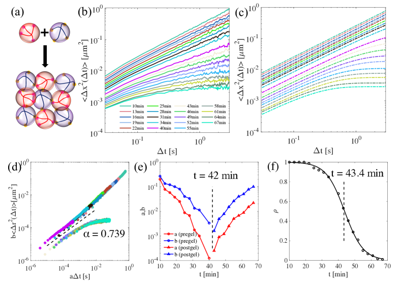
Figure 7: (a) Schematics showing the reaction between tetraPEG-SG and tetraPEGNH2. (b) Multiple particle tracking of the time series ensemble mean-squared displacement of the probes embedded in the mixed tetra-functional PEG plotted against lag time $\Delta t$. (c) AIUQ analysis of the same data as (b), denoted by the same color but with dotted lines. (d) Superposition of the data in (b) using MPT data. (e) Shift factors $a$ (red) and $b$ (blue) for pregel (circles), and postgel (triangles). (f) Estimated $\rho$ parameters in the OU process from a sequence of videos at different times denoted by black circles. The black solid line denotes the fit from a generalized logistic curve where $R^{2}_{adjusted}>0.99$.

A sol-gel transition is one where a solution is gradually transformed into a viscoelastic network, with progressively more solid-like characteristics. This phenomenon is observed in a number of naturally occurring polymers, such as collagen [69], protein solution [22], peptides [70] and silk fibrin [71]. Probing the timescale of the viscoelastic properties of the biopolymers can facilitate their use in reconstituted bioscaffolds.

Similarly, synthetic hydrogel materials with customized architecture can assemble into networks mimicking the mechanical properties and structure of their biological counterparts. Because of polyethylene glycol (PEG)’s inert properties, they are widely used as cell substrates [72], tissue scaffolds [73], and cell encapsulation applications [74]. Time-cure or time-concentration superposition analysis of microrheology experiments was introduced by Larsen and Furst [70]. To date, the tried-and-true method to determine gelling time from microrheology data is mostly done through shifting the MSD curves by hand [71, 75, 76].

The shifting is carried by multiplying the MSD curves and the $\Delta t$ by coefficients $a$ and $b$, determined through eyes. Once done, the MSD curves are collapsed into two distinct branches, one pre-gel and one post-gel. Each dataset (for a particular gelling time) should exhibit some degree of overlap with the subsequent one. The MSD at the gelling point is a critical curve between these two branches, which exhibits power-law-like behavior. The critical gelling exponent is defined as $\alpha=\frac{d\ln\langle\Delta x^{2}(\Delta t)\rangle}{d\ln\Delta t}$ [1, 70], where $\alpha$ is constant over all $\Delta t$, identical to the FBM model. Different systems experience gelation with distinct critical power-law exponents, as noted in [77]. These exponents can span from as high as $\alpha=0.88$ [78] to as low as $\alpha=0.16$ [75].

A recent approach [79] aimed to automate the process, using MSD versus $\Delta t$ curves estimated by MPT. However, these MSD curves are non-smooth and therefore extra efforts are required to smooth the MSD curves before implementing the superposition. DDM has also been utilized to explore gelation behaviors, although its use has typically been limited to an initial screening function, as demonstrated in [71]. One identifies gelation when displacement falls below a specific threshold, at which point it is challenging to analyze subtle displacements using DDM. In [22], the authors conducted MSD fitting using both MPT and DDM. They extracted the log-slope of MSD curves using MPT and subsequently fit a logit function to these slopes to identify gelation.

Here, we study the gelation of SG:NH2 = 1:1 tetraPEG mixtures. These functional groups react stoichiometrically to form highly regular networks (Fig 7(a)). Stock solutions for both 4-arm polyethylene glycol (PEG) polymers (100 mg/mL) were prepared to ensure that the sample was well-mixed. Due to the spontaneous nature of the SG-NH2 reaction, the reaction rate is entirely controlled by solution concentration, hence, we choose this system to benchmark the gelation time, which can be compared to previous study [80] with a reported gelation time of $\sim$ 44 min for a concentration of 20 mg/mL polymer. To counter hydrolysis, which is known to occur for SG groups dispersed in water, the 4-arm PEG-SG stock solution was prepared in DMSO. We first plot the estimated MSD by MPT in Fig. 7(b), which shows that the probe movements are initially diffusive, but at longer $T$, the probe motion becomes subdiffusive and the onset of a solid plateau begins to appear at longer $\Delta t$’s, meaning the particle becomes caged within the developing network.

The MSD curves from MPT are superposed by multiplying by a set of time shift factors $a$, and MSD shift factor $b$ to construct the master sol and gel curves in Fig. 7(d). By plotting $a$ and $b$ against time in Fig. 7(e), we approximate the gelation time to be $\approx$ 42 minutes, in good agreement with the reported gelling time $T_{gel}=44$ min [80]. However, it can be hard to determine the class of MSD curves close to the critical gelling curves, so the curves corresponding to the smallest shift factors are typically chosen, as shown in Fig. 7(e). Then the gelling point is defined as the time point when shift factors of the pre-gel and post-gel classes diverge, leading to the largest shift or changes between the curves.

Then we use AIUQ to automate the gelling point determination. The viscoelastic solid can be modeled by an OU process, with $\mbox{MSD}(\Delta t)=\sigma^{2}_{OU}(1-\rho^{\Delta t})$, which can capture the plateau and the reducing gradient of the MSD curve at large $\Delta t$’s. As the number of experiments is large, we use AIUQ with reduced $q$ for estimating the ISF. The estimated MSDs from the AIUQ approach with an OU model are shown in Fig. 7(c), which resemble curves from MPT curves from Fig. 7(b). The two parameters from the OU models, $\rho$ and $\sigma^{2}_{OU}$, determine the shape of the MSDs. This information can be further processed to deduce the gel point of the material. In Fig. 7(e), we plot the estimated parameter $\rho$ from the OU model for each experiment. The estimated $\rho$ gradually decreases, due to the caging effect from the network that traps particles at longer $\Delta t$’s. Before gelling, the absolute change of estimated $\rho$ increases, and the absolute change decreases after gelling. The rapid drop of $\rho$ from 1 to 0 indicates the sol-to-gel transition. To find the gelling point, we fit a generalized logistic function, $\rho(t)=\exp(-c_{1}(t-c_{2}))/(1+\exp(-c_{1}(t-c_{2})))$, where $c_{1}$ and $c_{2}$ are determined by minimizing a $L_{1}$ loss with respect to $\rho$. The $L_{2}$ loss is more robust than the $L_{2}$ loss, and here both give similar estimations. The fit is shown by the black solid line, which characterizes the change of $\rho$, and defines the gelling time to be the time point with the largest intermediate change in $\rho$. The inflection point is found to be 43.4 minutes using this fit, which is similar to the estimate $T_{gel}=44$ min in the previous study [80].

To extract the critical gelling exponent, we again compare two approaches. First, we plot the log shift factors $\log a$, $\log b$ against $\log$ of the extent of reaction $c$, defined as $c=\frac{|{T-T_{gel}}|}{T_{gel}}$, where $T_{gel}$ is the gelling time, hence $c$ determines distance to the gelling point [81]. Given $a\propto c^{-y}$, and $b\propto c^{-z}$, the scaling exponent is the ratio of these two exponents $\alpha=z/y$. This way, we obtain the scaling exponent for the tetraPEG-NH2 tetraPEG-SG system to be $\alpha$ = 0.739. The slope is plotted in Fig. 7(d) for reference. A second way is similar to what has been described in [22], the authors fit a logistic function to the relaxation exponent of the MSD. The same information can be obtained by fitting the fractional Brownian motion to all of the MSD curves, and we found that the critical exponent of $\alpha$ = 0.74 at gel point t = 43.4 min. Thus, the scattering analysis of microscopy by the AIUQ approach can be used to automatically extract the critical information of the systems, such as the gelling time and gelation property, removing the need of parameter tuning from MPT and shifting of MSD curves by hand.

The AIUQ approach provides an automated analysis of gelling time that extends the boundary of previous DDM techniques in the post-gel branch of the MSD for systems undergoing gelation [20, 22, 71]. Compared to MPT and conventional curve shifting for superposition by hand, AIUQ lifts the hurdles of strenuous analysis for a large number of videos by providing an automated estimation of gelling time and mechanical properties by AIUQ, which can be deployed for a sequences microscopy videos, at a given formulation and experiment condition (e.g. temperature, pH, etc). Along with high-throughput experiments, this data-processing technique can be integrated with Bayesian optimization and active learning approaches [82, 83] to optimize the compositions or material designs to achieve ideal gelling time and properties.

VI.4 Anisotropic diffusion in lyotropic LC

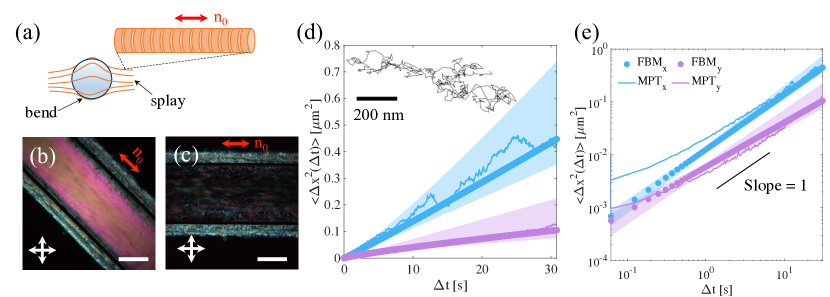
Figure 8: Anisotropic diffusion in DSCG. (a) Schematics of a probe particle moving amongst assembled stacks of DSCG, not drawn to scale. (b-c) Crossed-polarizer images when the channel is aligned either 45^o in (b) or parallel to the alignment direction of the channel in (c). The double-sided arrows denote the direction of the polarizer and analyzer. (d-e) Method comparisons between AIUQ fitting (filled circles) and MPT tracking (solid lines) of the image stack are presented in (d) lin-lin plot and (e) log-log plot. The inset in (d) shows an example particle trajectory. The shaded region denotes 95% confidence interval estimated using AIUQ reduced q.

Anisotropic motion is common in soft and biological systems containing passive particles or active agents, often due to the presence of anisotropic microstructures. An example can be seen in particles within an LC continuous phase. This leads to anisotropic particle motion, aligned either parallel or perpendicular to the orientation of the liquid crystal molecules. Here, we study the anisotropic motion of particles dispersed in lyotropic LC disodium cromoglycate (DSCG), where LC molecules self-assemble into rod-like structures (Fig. 8(a)). While traditionally used as an ingredient in allergy and asthma drugs [84], the current surge in interest in this organic salt as a biomaterial can be attributed to its lyotropic nature and biocompatibility [85, 86].

We disperse probes $2r_{p}=$ 200 nm at volume density $\phi$ = 8$\times 10^{-5}$ in 16 wt% DSCG solution. Given a density of 1.55 g/cm³ for pure DSCG [86], the solution density is 1.088 g/cm³ which is similar to that of polystyrene particles at 1.055 g/cm³ according to the manufacturer, hence these particles are neutrally buoyant. A small amount of surfactant (Triton X-100, 0.015 wt%) was added to prevent aggregation of the probes [87]. The capillary force upon filling is sufficient to ensure good alignment of the DSCG solution [88]. This concentration was chosen as its iso-nematic transition temperature is above room temperature so no isotropic to nematic transition occurred, as the iso-nematic fronts have been found to trap particles and cause aggregation. Uniform nematic alignment was obtained this way, as shown by the crossed-polarized images in Fig. 8(b)-(c). In these images, regions aligned parallel or perpendicular to the polarizer or analyzer direction appear dark, while other orientations appear bright.

An example of the anisotropic particle trajectory is shown in Fig. 8(d) inset. A probe particle moves predominantly along the x direction (sky blue) compared to y (purple). We estimate the MSDs by the MPT and AIUQ approach with a reduced number of $q$’s, while the estimation of AIUQ with all $q$ is similar. For AIUQ, we fit an FBM model to capture the large-$\Delta t$ behaviors of the anisotropic process, which mainly determines the diffusion coefficient in the previous study [88]. MSDs by MPT and AIUQ are shown in the lin-lin plot in Fig. 8(d) and then again in log-log in Fig. 8(e). Both MPT and AIUQ effectively capture the distinction in diffusion, in particular at long $\Delta t$’s. The estimated power parameter by the AIUQ is 1.04 and 0.83 for the x and y directions, respectively, which determine the slope of MSD in the log-log plot. Hence, while the motion along x can be described as mostly diffusive, the motion along y appears sub-diffusive, consistent with confinement in that direction due to structures imposed by ordered stacks of DSCG.

The nematic liquid crystal exhibits three primary modes of distortion: splay, twist, and bend. These modes correspond to the three Miesowicz viscosities, determined by solving the Ericksen-Leslie equations at low Ericksen numbers [89]. Splay and twist are readily understood in the distortion of the director field surrounding a colloid [90], or as depicted in Fig. 8(a). Earlier, the three Miesowicz viscosities of DSCG were measured using light scattering based on director fluctuations in [85], which found that the splay and twist viscosities are several orders of magnitudes higher than the bend viscosity. A more subdiffusive regime in the direction perpendicular to the director field has similarly been noted in [88] using particles of similar size. Despite a difference in particle size ($2r_{p}$ = 200 nm versus $\sim$6 $\mu$m), the estimated MSD also appears consistent with results presented in [87], which attributed the subdiffusive behavior to restoring forces on the particle, from incurred elastic free energy costs, partially offsetting the displacement from thermally driven fluctuations. A subdiffusive-to-diffusive transition was observed at the time scale of twist relaxation, which is on the order of $\Delta t\approx$ 100 s. In the range of observation (up to 30 s), the diffusion along y should be entirely sub-diffusive.

Finally, MSD from the MPT reveals a sub-diffusive regime of x direction for short $\Delta t$ as well. Subdiffusion in both the x and y directions has only been noted for particles diffusing in 4-cyano-4’-pentylbiphenyl (5CB) [91], a thermotropic liquid crystal. In the case of 5CB, the bend viscosity is only slightly lower than the splay and twist viscosities [85]. The notably low twist viscosity of DSCG is believed to exert a significant influence on particle motion [87], causing the discrepancy between thermotropic and lyotropic liquid crystals. Since FBM is used in the AIUQ approach, log-log plot of MSD over $\Delta t$ forms a straight curve according to the model assumption. Further analysis is needed to determine whether the observed sub-diffusive behavior is due to localization errors in MPT [12]. This problem may potentially be elucidated by either tracking a larger number of particles or employing two-point particle tracking microrheology, as described in [92, 88]. It quantifies the cross-correlated motion between a pair of tracers and is not influenced by the tracers’ size, shape, or their interaction with the local environment; instead, it relies on one tracer’s deformation affecting the motion of the other [92].

VII Discussion

Minimizing a loss function is often required for estimating parameters in physical and machine-learning approaches. Selecting the loss function and data regime or transformation of parameters implicitly reflects one’s probabilistic assumptions of data. We introduce a principled way to find a generative model for approaches that minimize a loss function in two steps. First, we construct a probabilistic model of the untransformed data from the beginning and show a loss-minimization approach is equivalent to a common statistical estimator of the generative model. Second, we integrate out the random component of the model to derive a more efficient estimator, such as the maximum marginal likelihood estimator herein, which naturally averages the information from different regimes of the transformed data. A generative model offers a probabilistic mechanism that allows for the derivation of the asymptotically optimal estimator, and the propagation of uncertainty from the initial stages of data analysis, which we term ab initio uncertainty quantification (AIUQ).

As an example, we derived a probabilistic generative model for DDM [14, 15], and show that the estimation in DDM analysis is equivalent to minimizing the temporal variogram of the projected intensity in the reciprocal space. Compared to tracking-based algorithms, DDM eliminates the need to track individual features, but selecting a range of wavevectors is still typically required in minimizing the loss function, which can differ in a case-by-case manner. With the probabilistic model of data, we derived the maximum marginal likelihood estimator of the parameters, which optimally weighs information at each wavevector, removing the need for selecting a wavevector range to analyze. By evoking the generalized Schur algorithm for Toeplitz covariance and further reducing data by truncating high-frequency wavevectors, we can accelerate the computation by around $10^{5}$ times for a microscopy video of regular size, compared to directly computing the likelihood function, allowing almost real-time analysis.

Through a variety of simulated studies of both isotropic and anisotropic processes, we found that the tuning-free AIUQ approach achieves a high estimation accuracy of model parameters and MSDs which were not seen before, justifying the efficiency in integrating the information at different wavevectors by the likelihood function. The $95\%$ confidence intervals of MSDs from the AIUQ estimation are typically narrow yet they cover the true MSDs at most $\Delta t$’s, indicating precise uncertainty quantification. Furthermore, using either the maximum likelihood value or predictive error, our method is able to correctly identify the true model amongst a few possible candidates using imaging data. This aspect had not been previously explored within this context.

The utility of the AIUQ approach was further studied in three distinct experiments. First, the AIUQ exhibits an advantage in analyzing optically dense systems filled with small particles in a Newtonian solution of polyvinyl alcohol, substantially outperforming MPT in estimating MSD. The advantage of analyzing the optically dense systems by DDM was found before [30], using a pre-selected range of wavevectors, whereas the AIUQ approaches can perform well with either reduced or all wavevectors. Second, we apply the AIUQ approach to automatically determine the gelation time and exponent during a sol-gel transition, where branched polymers grow to form volume-spanning networks. Over time, the mean squared displacement of the embedded particles falls below diffusive motion and acquires nonlinear characteristics, and exhibits critical behavior and divergence, and impacting various physical properties such as relaxation time and zero-shear viscosity [70]. We found that, while conventional methods to find the gel point often call for painstakingly shifting all curves so they line up on either the pre-gel or post-gel branch, AIUQ can automatically identify the gelation point, consistent with published data [80]. Third, we track the motion of nanoparticles diffusing in a uniformly aligned lyotropic liquid crystal. AIUQ effectively identifies the distinct migration pattern, including the diffusive behavior parallel to the director and the subdiffusive behavior of motion perpendicular to the director field. The latter can be attributed to elastic restoring force from the nematic liquid crystal.

Exploring particle dynamics opens up exciting avenues for mechanical testing, as highlighted in previous studies [1, 76]. AIUQ methods prove valuable in this context by generating smooth MSD, facilitating the connection of MSD data to frequency-dependent viscoelastic moduli using the Generalized Stokes-Einstein Relation (GSER) [93]. As demonstrated, using smaller videos, AIUQ estimation resulted in minimal loss of accuracy, enabling high spatial resolution by segmenting large videos [94]. Moreover, AIUQ methods hold promise for real-life suspensions, particularly those with multimodal particle size distributions [95] and spatially inhomogeneous samples [92]. Building upon the capacity to identify discrete anisotropic motion and super-, sub-diffusive dynamics, there lies an opportunity to extract the dynamics of active particles. AIUQ approaches are particularly suitable when individual agents do not have perfectly spherical shapes, making it applicable to analyzing actin dynamics [21], bacteria motion [18] and cell migration [35], which form large-scale coherent structures [96, 97] and undergo collective motion [98, 99]. Furthermore, AIUQ approaches remove the barrier of data processing as it does not require specifying a wavevector range to analyze, which is suitable for optimizing material properties, such as gelation time and property in high-throughput experiments from microscopy videos. Another application involves objects moving unidirectionally in flow [47], a common scenario in microfluidics. Flow-induced structures [100], lateral migration [101], or flow alignment [102], for instance, adds complexity to the dynamics. These observations necessitate an extension of the analysis framework beyond simple diffusive dynamics, and the estimation by the AIUQ approach can help understand the correlation pattern of anisotropic processes [49].

Finally, the AIUQ approach with a parametric model of ISF is a good complement to particle tracking approaches that produce MPT, enabling rigorous model comparison and hypothesis testing. Because the ISF can be approximated using MSD by the cumulant theorem, this becomes particularly intriguing in cases where the underlying model governing the dynamic process is unknown [20, 23]. As model-free DDM proceeds by directly inverting the ISF separately at each $\Delta t$, inevitably truncating $\Delta t$’s that cannot be reliably analyzed. Consequently, one can be left with a range of $\Delta t$’s much shorter than that from MPT. Rather, the ISF approximated by MSD can be optimized using the likelihood function in Eq. (9) to efficiently weigh all information at different wavevectors and lag time. To overcome the challenge of optimizing a large number of MSD on all lag times, one may optimize the MSD at a few equally spaced lag times, then reconstruct the MSD on all lag times by Gaussian process regression [103]. The use of the likelihood function in Eq. (9) can substantially improve the efficiency of a similar approach in [23] by minimizing the loss based on the ISF.

VIII Acknowledgements

This project is partially supported by the National Science Foundation under Grant No. DMS-2053423. MG acknowledges the supplement to National Science Foundation Grant No. 2119663. YH acknowledges partial support from the UC Multicampus Research Programs and Initiatives (MRPI) program under Grant No. M23PL5990 and from the BioPACIFIC Materials Innovation Platform of the National Science Foundation under Grant No. DMR-1933487 (NSF BioPACIFIC MIP). YL acknowledges support from the Biological Sciences Postdoctoral Fellowship Program from Yale Provost’s office. The authors thank Matthew Helgeson, Ryan McGorty, Rae Robertson-Anderson and Megan Valentine for helpful discussions.

Appendices

Appendix A: Derivation for Section II

The intermediate scattering function (ISF) defined in Eq. (2) is computed by

$$f_{\bm{\theta}}(\mathbf{q},\Delta t)$$

$$= \mbox{Cov}(\psi(\mathbf{q},t),\psi^{*}(\mathbf{q},t+\Delta t))$$

$$= \mathbb{E}[\psi(\mathbf{q},t)\cdot\psi^{*}(\mathbf{q},t+\Delta t)]$$

$$= \mathbb{E}\left[\frac{1}{M}\sum^{M}_{m=1}\exp\left(i\mathbf{q}\cdot(\mathbf{x}_{m}(t+\Delta t)-\mathbf{x}_{m}(t))\right)\right]+$$

$$\qquad\mathbb{E}\left[\frac{1}{M}\sum_{j\neq j^{\prime}}\exp\left(i\mathbf{q}\cdot(\mathbf{x}_{j}(t+\Delta t)-\mathbf{x}_{j^{\prime}}(t))\right)\right]$$

$$= \Bigl{<}\frac{1}{M}\sum^{M}_{m=1}\exp\left(i\mathbf{q}\cdot\Delta\mathbf{x}_{m}(t,\Delta t)\right)\Bigr{>}.$$

The last equation holds because there is no interaction between particles and the long-term expectation of $\psi$ is zero by assumption [16]. Note that the derivation of ISF assumes the particle intensity profile is a Dirac delta function, which does not strictly hold in light microscopy. Consequently, the amplitude is relevant to various factors, such as the structure factor and the particle form factor [50] and they typically need to be estimated.

As all particles have the same displacement distributions, the ISF of 2D processes can be written as

$$f_{\bm{\theta}}(\mathbf{q},\Delta t) =\mathbb{E}\left[\exp\left(i\mathbf{q}\cdot\Delta\mathbf{x}(t,\Delta t)\right)\right]$$

$$=\mathbb{E}\left[\exp\left(iq_{1}\Delta x_{1}(t,\Delta t)\right)\right]\mathbb{E}\left[\exp\left(iq_{2}\Delta x_{2}(t,\Delta t)\right)\right]$$

$$:=f_{\bm{\theta}_{1}}(q_{1},\Delta t)f_{\bm{\theta}_{2}}(q_{2},\Delta t).$$ (A1)

Based on the cumulant generating function, for any $l=1,2$, we have a power series expansion of the ISF [104, 31],

$$\log(f_{\bm{\theta}_{l}}(q_{l},\Delta t))=\sum^{\infty}_{j=1}\kappa_{l,j}\frac{(iq_{l})^{j}}{j!},$$ (A2)

where $\kappa_{l,j}=f^{(j)}_{\bm{\theta}_{l}}(q_{l},0)$ is the $j$th derivative of the ISF with respect to the random displacement along the $l$th coordinate at time $\Delta t$. Note that $\kappa_{l,1}=\mathbb{E}[\Delta x_{l}(t,\Delta t)]$ and $\kappa_{l,2}=\mathbb{E}[\Delta x_{l}(t,\Delta t)^{2}]$ are first and second moments, respectively. As the first moment is zero, approximating the log ISF along the $l$th coordinate by the first two moments follows

$$\log(f_{\bm{\theta}_{l}}(q_{l},\Delta t))\approx\frac{-q^{2}_{l}\mathbb{E}[\Delta x^{2}_{l}(t,\Delta t)]}{2}.$$ (A3)

Substitute $f_{l}(q_{l},\Delta t)$ from Eq. (A3) into (A1) gives an approximation of the ISF by the MSD in a 2D space:

$$f_{\bm{\theta}}(\mathbf{q},\Delta t)$$

$$\approx \exp\left\{-\frac{1}{2}\mathbb{E}\left[q^{2}_{1}\Delta x^{2}_{1}(t,\Delta t)+q^{2}_{2}\Delta x^{2}_{2}(t,\Delta t)\right]\right\}$$ (A4)

$$= \exp\left\{-\frac{1}{4}\mathbb{E}\left[(q^{2}_{1}+q^{2}_{2})(\Delta x^{2}_{1}(t,\Delta t)+\Delta x^{2}_{2}(t,\Delta t))\right]\right\}$$

$$= \exp\left(-\frac{q^{2}\Delta x^{2}(\Delta t)}{4}\right),$$

where $q^{2}=q^{2}_{1}+q^{2}_{2}$ and the MSD $\Delta x^{2}(\Delta t)=\Delta x^{2}_{1}(t,\Delta t)+\Delta x^{2}_{2}(t,\Delta t)$.

Parametric	ISF
BM	$\exp\left(-q^{2}\sigma^{2}_{BM}\Delta t/4\right)$
FBM	$\exp\left(-q^{2}\sigma^{2}_{FBM}\Delta t^{\alpha}/4\right)$
OU	$\exp\left(-q^{2}\sigma^{2}_{OU}(1-\rho^{\Delta t})/4\right)$
OU$+$FBM	$\exp\left(-q^{2}(\sigma^{2}_{1}\Delta t^{\alpha}+\sigma^{2}_{2}(1-\rho^{\Delta t}))/4\right)$
Nonparametric	ISF
Cumulant approx.	$\exp\left(-q^{2}\langle\Delta x^{2}(\Delta t)\rangle/4\right)$

Table 3: A list of parametric models of the intermediate scattering function (ISF) for Brownian motion (BM), fractional Brownian motion (FBM), Ornstein–Uhlenbeck (OU) process, and a mixture of the OU process and FBM (OU$+$FBM). The nonparametric model uses cumulant approximation [31] to construct the ISF by the mean squared displacement $\langle\Delta x^{2}(\Delta t)\rangle$, which gives a unique parameter at any lag time $\Delta t$.

ISFs of a few widely used processes are summarized in Table 3, which follows from approximation by MSD. For a Brownian motion (BM), for instance, the update of the 2D position of the $m$th particles follows $\mathbf{x}_{m}(t+\Delta t_{min})=\mathbf{x}_{m}(t)+\frac{\sigma^{2}_{BM}}{2}\bm{\epsilon}_{m}(t)$ with $\bm{\epsilon}_{m}(t)\sim\mathcal{MN}(\mathbf{0},\mathbf{I}_{2})$. The MSD of BM follows $\mbox{MSD}_{BM}=\sigma^{2}_{BM}\Delta t$ [23].

For an OU process, the particle’s successive steps have a weaker correlation with previous steps than the BM,

$$\mathbf{x}_{m}(t+\Delta t_{min}) =\rho(\mathbf{x}_{m}(t)-\mathbf{x}_{m}(t_{1}))+\mathbf{x}_{m}(t_{1})$$

$$\quad\quad+\frac{\sigma_{OU}^{2}(1-\rho^{2})}{4}\bm{\epsilon}_{m}(t),$$ (A5)

where $\mathbf{x}_{m}(t_{1})\sim\mathcal{MN}(\mathbf{x}_{m}(t_{0}),\frac{\sigma_{OU}^{2}}{4}\mathbf{I}_{2})$, for a deterministic position $\mathbf{x}_{m}(t_{0})$. The MSD of the OU process follows $\sigma_{OU}^{2}(1-\rho^{\Delta t})$ [23].

We introduce the MSD and derivation for two other processes: the fractional Brownian motion (FBM), and a mixture of the OU process and FBM, which the same MSD as the continuous time random walk (CTRW) and the noisy continuous time random walk (NCTRW), respectively [105, 106]. Denote $\Delta n=\Delta t/\Delta t_{min}$. First, simulated particles from a 2D FBM process exhibit long-term dependence, and the self-similarity is controlled by the Hurst parameter $H=\alpha/2$ [107, 108]:

$$x_{m,l}(t+\Delta t)=x_{m,l}(t)+\sum_{k=0}^{\Delta n-1}\tilde{x}_{m,l}(t_{k}),$$ (A6)

where the incremental process $\tilde{x}_{m,l}(t_{k})=x_{m,l}(t_{k}+\Delta t_{min})-x_{m,l}(t_{k})$ is known as the fractional Gaussian noise with $\mathbb{E}\left[\tilde{x}_{m,l}(t_{k})\right]=0$, and $\operatorname{Cov}\left(\tilde{x}_{m,l}(t_{k}),\tilde{x}_{m,l}(t_{s})\right)=\frac{\sigma_{FBM}^{2}}{4}\left(|t_{k}|^{2H}+|t_{s}|^{2H}-2|t_{k}-t_{s}|^{2H}\right)$; the indices representing the $m$th particle and $l$th direction ($l=1,2$). For any $\mathbf{x}(t+\Delta t)$, $\mathbf{x}(t)\in\mathbb{R}^{2}$, the MSD for FBM can be computed as

$$\mathbb{E}\left[\left(x_{m,l}(t+\Delta t)-x_{m,l}(t)\right)^{2}\right]$$

$$= \mathbb{V}\left[x_{m,l}(t+\Delta t)-x_{m,l}(t)\right]+\mathbb{E}^{2}\left[x_{m,l}(t+\Delta t)-x_{m,l}(t)\right]$$

$$= \mathbb{V}\left[\sum_{k=0}^{\Delta n-1}\tilde{x}_{m,l}(t+k\Delta t_{min})\right],$$

for any particle $m=1,\dots,M$ and coordinate $l=1,2$. It’s not hard to show that for any $\Delta t$[108]:

$$\mathbb{V}\left[\sum_{k=0}^{\Delta n-1}\tilde{x}_{m,l}(t+k\Delta t_{min})\right]=\frac{\sigma_{FBM}^{2}}{2}\Delta t^{2H}=\frac{\sigma_{FBM}^{2}}{2}\Delta t^{\alpha}.$$ (A7)

Since particles move isotropically in a 2D space, the MSD for FBM is $\mathbb{E}\left[\Delta x^{2}(\Delta t)\right]=\sigma_{FBM}^{2}\Delta t^{\alpha}$.

We next consider particles undergoing a mixture of the OU process and FBM. This model presents a generalized form of FBM or the continuous time random walk [106]. This extension is suitable for describing scenarios where the particles are confined within cages and exhibit waiting times distributed according to power laws. Here, the process can be simulated through a summation of a mutually independent FBM and an OU process. The update of the particles’ position follows

$$x_{m,l}(t)=u_{m,l}(t)+v_{m,l}(t)$$ (A8)

where $u_{m,l}(t)$ is a FBM process in the $l$th direction with MSD $\sigma^{2}_{1}\Delta t^{\alpha}/2$, and $v_{i,l}(t)$ stands for an independent OU process in the $l$th direction with MSD $\sigma^{2}_{2}(1-\rho^{\Delta t})/2$. Since particles move isotropically in a 2D space, and the two processes are independent, the MSD is $\sigma^{2}_{1}\Delta t^{\alpha}+\sigma_{2}^{2}(1-\rho^{\Delta t})$.

Appendix B: Derivation for Section III

We first derive the distribution of $\Delta{\hat{y}}_{re,\mathbf{q}}(t,\Delta t)$ and the distribution of $\Delta{\hat{y}}_{im,\mathbf{q}}(t,\Delta t)$ can be shown similarly. Note $\mathbb{E}[\Delta{\hat{y}}_{re,\mathbf{q}}(t,\Delta t)]=0$. The variance can be computed by

$$\mathbb{V}[\Delta{\hat{y}}_{re,\mathbf{q}}(t,\Delta t)]$$

$$= \mathbb{V}[{\hat{y}}_{re,\mathbf{q}}(t+\Delta t)]+\mathbb{V}[{\hat{y}}_{re,\mathbf{q}}(t)]$$

$$\qquad-2\mbox{Cov}[{\hat{y}}_{re,\mathbf{q}}(t),{\hat{y}}_{re,\mathbf{q}}(t+\Delta t)]$$

$$= 2\times\frac{A(\mathbf{q})}{4}+2\times\frac{\bar{B}}{4}-2\times\frac{A(\mathbf{q})}{4}f_{\bm{\theta}}(\mathbf{q},\Delta t)$$

$$= \frac{A(\mathbf{q})}{2}(1-f_{\bm{\theta}}(\mathbf{q},\Delta t))+\frac{\bar{B}}{2}.$$

As $\Delta{\hat{y}}_{re,\mathbf{q}}(t,\Delta t)$ follows a Gaussian distribution, we have $\Delta{\hat{y}}_{re,\mathbf{q}}(t,\Delta t)\sim\mathcal{N}\left(0,\frac{A(\mathbf{q})}{2}\left(1-f_{\bm{\theta}}(\mathbf{q},\Delta t)\right)+\frac{\bar{B}}{2}\right)$.

We next derive the probability density of $J$ rings of transformed intensity at the Fourier space in Eq. (9). From Eq. (6), the mean of an $n$-vector $\mathbf{y}_{j^{\prime},re}=(y_{j^{\prime},re}(t_{1}),...,y_{j^{\prime},re}(t_{n}))^{T}$ for any $j^{\prime}\in\mathcal{S}_{j}$ can be computed by the law of total expectation below:

$$\mathbb{E}[\mathbf{y}_{j^{\prime},re}]=\mathbb{E}[\mathbb{E}[\mathbf{y}_{j^{\prime},re}\mid\mathbf{z}_{re,j^{\prime}}]]=\mathbb{E}[\mathbf{z}_{re,j^{\prime}}]=\mathbf{0},$$

where $\mathbf{z}_{re,j^{\prime}}=(z_{re,j^{\prime}}(t_{1}),...,z_{re,j^{\prime}}(t_{n}))^{T}$ is a vector of zero-mean, real-valued random factors. The covariance of $\mathbf{y}_{re,j^{\prime}}$ can be computed by the law of total covariance:

$$\mathbb{V}[\mathbf{y}_{re,j^{\prime}}] =\mathbb{V}[\mathbb{E}[\mathbf{y}_{re,j^{\prime}}\mid\mathbf{z}_{re,j^{\prime}}]]+\mathbb{E}[\mathbb{V}[\mathbf{y}_{re,j^{\prime}}\mid\mathbf{z}_{re,j^{\prime}}]]$$

$$=\mathbb{V}[\mathbf{z}_{re,j^{\prime}}]+\frac{\bar{B}}{4}\mathbf{I}_{n}=\frac{A_{j}}{4}\mathbf{R}_{j}+\frac{\bar{B}}{4}\mathbf{I}_{n}.$$

Note that $\mathbf{y}_{re,j^{\prime}}$ is Gaussian since both $\mathbf{z}_{re,j^{\prime}}$ and $\bm{\epsilon}_{j,re}=(\bm{\epsilon}_{j,re}(t_{1}),...,\bm{\epsilon}_{j,re}(t_{n}))^{T}$ are Gaussian. Furthermore, the random factors $\mathbf{z}_{re,j^{\prime}_{1}}$ and $\mathbf{z}_{re,j^{\prime}_{2}}$ are independent when $j^{\prime}_{1}\neq j^{\prime}_{2}$, and the noise is also independent. Hence the probability density of $\tilde{N}\times n$ matrix $\mathbf{\hat{y}}_{re}=[\mathbf{\hat{y}}_{re}(t_{1}),...,\mathbf{\hat{y}}_{re}(t_{n})]$ follows

$$p(\mathbf{\hat{y}}_{re}\mid\bm{\theta},\mathbf{A}_{1:J},\bar{B})=\prod^{J}_{j=1}\prod_{j^{\prime}\in\mathcal{S}_{j}}p_{MN}\left(\mathbf{\hat{y}}_{re,j^{\prime}};\,\mathbf{0},\,\bm{\Sigma}_{j}\right).$$

As the density of the imaginary part can be similarly derived, we have the logarithm of the likelihood below

$$\log(\mathcal{L}\left(\bm{\theta},\bm{A}_{1:J},\bar{B}\right))$$

$$= -{n\tilde{N}}\mbox{log}(2\pi)-\sum^{J}_{j=1}\left\{{S_{j}}\log(|\bm{\Sigma}_{j}|)\right\}$$

$$-\frac{S_{j}}{2}\sum_{j^{\prime}\in\mathcal{S}_{j}}\big{(}\mathbf{\hat{y}}_{re,j^{\prime}}^{T}\bm{\Sigma}_{j}^{-1}\mathbf{\hat{y}}_{re,j^{\prime}}+\mathbf{\hat{y}}_{im,j^{\prime}}^{T}\bm{\Sigma}_{j}^{-1}\mathbf{\hat{y}}_{im,j^{\prime}}\big{)},$$ (A9)

which is the density of the right-hand-side of Eq. (9).

Appendix C: Toeplitz matrix and generalized Schur algorithm

Here we summarize the general ideas and the general Schur algorithm for accelerating the computation of the inversion and determinant of the Toeplitz covariance. For ease of notation, we drop subscript $j$ in the Toeplitz matrix $\bm{\Sigma}_{j}$ in Eq. (9) and the result applies to all $j$. In [109], the inversion of the Toeplitz matrix $\bm{\Sigma}$ was shown to be the difference between two matrices, where each matrix follows a product of a lower triangular Toeplitz matrix and an upper triangular Toeplitz matrix:

$$\bm{\Sigma}^{-1}=\frac{1}{\delta_{n-1}}\left(\mathbf{L}_{1}\mathbf{L}_{1}^{T}-\mathbf{L}_{0}\mathbf{L}_{0}^{T}\right),$$ (A10)

where

$$\small{\mathbf{L}_{0}=\begin{bmatrix}0&&&&\\ \phi_{2}&0&&&\\ \phi_{3}&\phi_{2}&\ddots&&\\ \vdots&\vdots&\ddots&\ddots&\\ \phi_{n}&\phi_{n-1}&\dots&\phi_{2}&0\\ \end{bmatrix}},\small{\mathbf{L}_{1}=\begin{bmatrix}1&&&&\\ \phi_{n}&1&&&\\ \phi_{n-1}&\phi_{n}&\ddots&&\\ \vdots&\vdots&\ddots&\ddots&\\ \phi_{2}&\phi_{3}&\dots&\phi_{n}&1\\ \end{bmatrix}},\quad$$

with $\bm{\phi}=(\phi_{1},\dots,\phi_{n})^{T}=(0,\eta_{n-1,n-1},\cdots,\eta_{n-1,1})^{T}+(\xi_{n-1,n-1},\cdots,\xi_{n-1,1},0)^{T}$ and $\delta_{n-1}$ is a constant determined by $\bm{\Sigma}$ uniquely.

We summarize the generalized Schur algorithm [52, 54] in Algorithm 1 and Algorithm 2 for computing $\bm{\xi}_{n-1}^{(n-1)}=(\xi_{n-1,1},...,\xi_{n-1,n-1})^{T}$, $\bm{\eta}_{n-1}^{(n-1)}=(\eta_{n-1,1},...,\eta_{n-1,n-1})^{T}$ and the so-called Schur parameters $\{\gamma_{k}\}_{k=1}^{n-1}$ recursively. Algorithm 1 is initialized by $\bm{\alpha}_{0}^{(n-1)}=-(\tilde{f}_{0},\tilde{f}_{1}\dots\tilde{f}_{n-2})$ and $\bm{\beta}_{0}^{(n-1)}=(\tilde{f}_{1},\tilde{f}_{1}\dots\tilde{f}_{n-1})$ from the Toeplitz covariances in Eq. (12), and Algorithm 2 is called for even numbers of observations, enabling the approach to be applicable to any number of observations. For both algorithms, we let $\bm{\alpha}^{(d_{p})}_{p}$, $\bm{\beta}^{(d_{p})}_{p}$, $\bm{\xi}^{(d_{p})}_{p}$ and $\bm{\eta}^{(d_{p})}_{p}$ denote length $d_{p}$ coefficients vectors under recursion index $p$, associated with Algorithm 2 when started with inputs $\bm{\alpha}_{0}^{(.)}$, $\bm{\beta}_{0}^{(.)}$. We also denote $\bm{\xi}_{p,d_{p}}$, $\bm{\eta}_{p,d_{p}}$ the $d_{p}$ vectors from Algorithm 2 if provided with inputs $\bm{\alpha}_{p}^{d_{p}}$, $\bm{\beta}_{p}^{d_{p}}$. Correspondingly, we denote $\alpha^{(d_{p})}_{p}(\nu)=\sum_{d=1}^{d_{p}}\alpha_{p,d}\nu^{d-1}$, $\beta^{(d_{p})}_{p}(\nu)=\sum_{d=1}^{d_{p}}\beta_{p,d}\nu^{d-1}$, $\xi^{(d_{p})}_{p}(\nu)=\sum_{d=1}^{d_{p}}\xi_{p,d}\nu^{d-1}$, $\eta^{(d_{p})}_{p}(\nu)=\sum_{d=1}^{d_{p}}\eta_{p,d}\nu^{d-1}$, $\xi_{p,d_{p}}(\nu)=\sum_{d=1}^{d_{p}}\xi_{p,d_{p},d}\nu^{d-1}$ and $\eta_{p,d_{p}}(\nu)=\sum_{d=1}^{d_{p}}\eta_{p,d_{p},d}\nu^{d-1}$ as polynomials of degree $d_{p}$ with input $\nu$ and the coefficients $\alpha_{p,d}$, $\beta_{p,d}$, $\xi_{p,d}$, $\eta_{p,d}$, $\xi_{p,d_{p},d}$, $\eta_{p,d_{p},d}$ being the $d$th entry of $\bm{\alpha}^{(d_{p})}_{p}$, $\bm{\beta}^{(d_{p})}_{p}$, $\bm{\xi}^{(d_{p})}_{p}$, $\bm{\eta}^{(d_{p})}_{p}$, $\bm{\xi}_{p,d_{p}}$ and $\bm{\eta}_{p,d_{p}}$ for $d=1,\ldots,d_{p}$. The conjugate polynomials of $\xi^{(d_{p})}_{p}(\nu)$ and $\eta^{(d_{p})}_{p}(\nu)$ are defined as $\tilde{\xi}^{(d_{p})}_{p}(\nu)=\nu^{2}\xi^{(d_{p})}_{p}(1/\nu)$ and $\tilde{\eta}^{(d_{p})}_{p}(\nu)=\nu^{2}\eta^{(d_{p})}_{p}(1/\nu)$. Hereafter, the multiplications between two polynomials are considered convolution and can be computed efficiently via FFT. Furthermore, the determinant of $\bm{\Sigma}$ can be efficiently computed as well:

$$|\bm{\Sigma}|=\tilde{f}_{0}\prod_{k=1}^{n-1}\delta_{k},$$ (A11)

where $\delta_{k}=\tilde{f}_{0}\prod_{i=1}^{k}(1-\gamma_{k}^{2})$ for $k=1,\ldots,n-1$ [26] with $\tilde{f}_{0}$ being the first diagonal element of $\bm{\Sigma}$ and $\delta_{n-1}$ employed in Eq. (A10).

Algorithm 1 The generalized Schur algorithm for arbitrary integer $n>1$.

Function GSCHUR

1. Input: $\bm{\alpha}_{0}^{(n-1)}=-(\tilde{f}_{0},\tilde{f}_{1}\dots\tilde{f}_{n-2})^{T}$ and $\bm{\beta}_{0}^{(n-1)}=(\tilde{f}_{1},\tilde{f}_{1}\dots\tilde{f}_{n-1})^{T}$. Decompose $n=1+n_{1}+n_{2}+\dots+n_{N_{r}}$, with $n_{1}=2^{r_{1}},\ldots,n_{N_{r}}=2^{r_{N_{r}}}$ for non-negative integers $(r_{1},\dots,r_{N_{r}})$.

2. Update $m=n_{1}$, and do ($\bm{\xi}_{m}^{(m)}$, $\bm{\eta}_{m}^{(m)}$, $\{\gamma_{k}\}_{k=1}^{m}$) = GSCHUR2($\bm{\alpha}_{0}^{(m)}$, $\bm{\beta}_{0}^{(m)}$) defined in Algorithm 2.

3. For $j=2,...,N_{r}$: Let $m_{j}=n_{j}$, then (i) Compute the product below via FFT,

$$\begin{bmatrix}\alpha_{m}^{(m_{j})}(\nu)\\ \beta_{m}^{(m_{j})}(\nu)\end{bmatrix}\longleftarrow\frac{1}{\nu^{m}}\begin{bmatrix}\eta_{m}^{(m)}(\nu)&-\xi_{m}^{(m)}(\nu)\\ -\tilde{\xi}_{m}^{(m)}(\nu)&\tilde{\eta}_{m}^{(m)}(\nu)\end{bmatrix}\begin{bmatrix}\alpha_{0}^{(m+m_{j})}(\nu)\\ \beta_{0}^{(m+m_{j})}(\nu)\end{bmatrix},$$

The multiplication on the right-hand side yields two polynomials of degree $2m+m_{j}$, while $\alpha_{m}^{(m_{j})}(\nu)$ and $\beta_{m}^{(m_{j})}(\nu)$ are polynomials of degree $m_{j}$ by only retaining the middle $m_{j}$ coefficients from the multiplication. (ii) Use the function ($\bm{\xi}_{m,m_{j}},\bm{\eta}_{m,m_{j}},\{\gamma_{k}\}_{k=m+1}^{m+m_{j}}$) = GSCHUR2($\bm{\alpha}_{m}^{(m_{j})}$, $\bm{\beta}_{m}^{(m_{j})}$). (iii) Compute the following product via FFT

$$\begin{bmatrix}\xi_{m+m_{j}}(\nu)\\ \eta_{m+m_{j}}(\nu)\end{bmatrix} =\begin{bmatrix}\tilde{\eta}_{m}^{(m)}(\nu)&\xi_{m}^{(m)}(\nu)\\ \tilde{\xi}_{m}^{(m)}(\nu)&\eta_{m}^{(m)}(\nu)\end{bmatrix}\begin{bmatrix}\xi_{m,m_{j}}(\nu)\\ \eta_{m,m_{j}}(\nu)\end{bmatrix},$$

and update $\{\gamma_{k}\}_{k=1}^{m+m_{j}}=(\{\gamma_{k}\}_{k=1}^{m},\{\gamma_{k}\}_{k=m+1}^{m+m_{j}})$. (iv) Update $m=m+m_{j}$. End for

4. Output: $\bm{\xi}_{n-1}^{(n-1)}$, $\bm{\eta}_{n-1}^{(n-1)}$, and $\{\gamma_{k}\}_{k=1}^{n-1}$.

Algorithm 2 Schur for even $m_{j}$ from Algorithm 1.

Function GSCHUR2

1. Input: vectors $\bm{\alpha}_{m}^{(m_{j})}$ and $\bm{\beta}_{m}^{(m_{j})}$. Initialize polynomials $\xi_{1}^{(1)}(\nu)=\gamma_{1}^{(1)}(\nu)=\alpha_{m}^{(1)}(\nu)/\beta_{m}^{(1)}(\nu)$, and let $\eta_{1}^{(1)}(\nu)=1$. Obtain $\tilde{\xi}_{1}^{(1)}(\nu)=\nu^{2}\xi_{1}^{(1)}(1/\nu)$ and $\tilde{\eta}_{1}^{(1)}(\nu)=\nu^{2}\eta_{1}^{(1)}(1/\nu)$.

2. For $p=1,2,...,\frac{m_{j}}{2}$: (i) Compute the following product via FFT

$$\begin{bmatrix}\alpha_{p}^{(p)}(\nu)\\ \beta_{p}^{(p)}(\nu)\end{bmatrix}\longleftarrow\frac{1}{\nu^{p}}\begin{bmatrix}\eta_{p}^{(p)}(\nu)&-\xi_{p}^{(p)}(\nu)\\ -\tilde{\xi}_{p}^{(p)}(\nu)&\tilde{\eta}_{p}^{(p)}(\nu)\end{bmatrix}\begin{bmatrix}\alpha_{0}^{(2p)}(\nu)\\ \beta_{0}^{(2p)}(\nu)\end{bmatrix},$$

Multiplying polynomials on the right-hand side yields two polynomials of degree $3p$, while $\alpha_{p}^{(p)}(\nu)$ and $\beta_{p}^{(p)}(\nu)$ are polynomials of degree $p$ by only retaining the middle $p$ coefficients from the yielded polynomials. (ii) Get $\bm{\xi}_{p,p}$ and $\bm{\eta}_{p,p}$ from $\bm{\alpha}_{p}^{(p)}$ and $\bm{\beta}_{p}^{(p)}$ by running ($\bm{\xi}_{p,p}$, $\bm{\eta}_{p,p}$, $\{\gamma_{k}\}_{k=p+1}^{2p}$) = GSCHUR2($\bm{\alpha}_{p}^{(p)}$, $\bm{\beta}_{p}^{(p)}$). (iii) Compute the following product via FFT

$$\begin{bmatrix}\xi_{2p}(\nu)\\ \eta_{2p}(\nu)\end{bmatrix}=\begin{bmatrix}\tilde{\eta}_{p}^{(p)}(\nu)&\xi_{p}^{(p)}(\nu)\\ \tilde{\xi}_{p}^{(p)}(\nu)&\eta_{p}^{(p)}(\nu)\end{bmatrix}\begin{bmatrix}\xi_{p,p}(\nu)\\ \eta_{p,p}(\nu).\end{bmatrix}$$

End for

3. Output: $\bm{\xi}_{m_{j}}^{(m_{j})}$, $\bm{\eta}_{m_{j}}^{(m_{j})}$, and $\{\gamma_{k}\}_{k=1}^{m_{j}}$.

We highlight the computational advantages of the generalized Schur algorithm. First, it only requires $\mathcal{O}(\sum_{i=1}^{N_{r}}n_{i}\log^{2}n_{i})$ operations to get $\bm{\xi}_{n-1}^{(n-1)}$, $\bm{\eta}_{n-1}^{(n-1)}$ and $\{\gamma_{k}\}_{k=1}^{n-1}$, by decomposing $n=1+n_{1}+\dots+n_{N_{r}}$ as a series of powers of 2, i.e. $n_{i}=2^{r_{i}}$ for an integer $r_{i}\geq 0$. In practice, we can limit the integer $r_{i}\leq 6$ to control the burden of calculation for each recursion. And after obtaining $\{\gamma_{k}\}_{k=1}^{n-1}$, the log determinant of the Toeplitz covariance in Eq. (A11) can be computed in $\mathcal{O}(n)$ operations. Second, according to Eq. (A10), the matrix-vector multiplication follows

$$\bm{\Sigma}^{-1}\mathbf{v}=\frac{1}{\delta_{n-1}}\left(\mathbf{L}_{1}\mathbf{L}_{1}^{T}-\mathbf{L}_{0}\mathbf{L}_{0}^{T}\right)\mathbf{v},$$ (A12)

where $\mathbf{L}_{0}$, $\mathbf{L}_{0}^{T}$, $\mathbf{L}_{1}$ and $\mathbf{L}_{1}^{T}$ are all Toeplitz matrices. A lower triangular Toeplitz matrix, such as $\mathbf{L}_{0}$, can be embedded into a circulant matrix $\tilde{\mathbf{L}}_{0}$ of size $2n$:

$$\small{\tilde{\mathbf{L}}_{0}=\begin{bmatrix}0&&&&&0&\phi_{n}&\dots&\phi_{3}&\phi_{2}\\ \phi_{2}&0&&&&\phi_{n}&\ddots&\ddots&&\phi_{3}\\ \phi_{3}&\phi_{2}&\ddots&&&\ddots&\ddots&\ddots&\vdots&\\ \vdots&\vdots&\ddots&\ddots&&\phi_{3}&\ddots&\ddots&\vdots&\phi_{n-1}\\ \phi_{n}&\phi_{n-1}&\dots&\phi_{2}&0&\phi_{2}&\phi_{3}&\ddots&\phi_{n-1}&0\\ 0&\phi_{n}&\dots&\dots&\phi_{2}&0&&&&\\ \phi_{n}&\ddots&\ddots&&\phi_{3}&\phi_{2}&0&&&\\ \vdots&\ddots&\ddots&\phi_{n}&\vdots&\phi_{3}&\phi_{2}&\ddots&&\\ \vdots&&&\ddots&\vdots&\vdots&&\ddots&\ddots&\\ \phi_{2}&\phi_{3}&\ddots&&0&\phi_{n}&\phi_{n-1}&\dots&\phi_{2}&0\\ \end{bmatrix}.}$$ (A13)

Processes,	Small video					Regular video
RMSE of MSD	DDM	DDM	AIUQ	AIUQ	MPT	DDM	DDM	AIUQ	AIUQ	MPT
	fixed	opt	reduction	all		fixed	opt	reduction	all
Slow BM	480	20	0.017	0.023	0.17	800	160	0.15	0.14	0.34
Fast BM	100	19	3.4	3.7	14	460	240	7.7	7.8	100
FBM, subdiff	63	180	1.9	2.0	60	690	330	6.7	6.7	37
FBM, superdiff	290	51	5.5	5.6	55	4500	1200	72	77	570
OU	$5.6\times 10^{5}$	51	2.0	2.0	120	$6.9\times 10^{4}$	40	2.9	3.0	17
OU$+$FBM	450	100	2.2	2.2	28	2200	140	0.90	0.91	8.5

Table 4: RMSE of estimated MSD by DDM, AIUQ and MPT for 6 simulated isotropic processes with small and regular-size videos in Section V.1. The order of the process is arranged as the same as Table 1.

The eigendecomposition of $\tilde{\mathbf{L}}_{0}$ follows $\tilde{\mathbf{L}}_{0}=\mathbf{F}^{-1}\bm{\Lambda}\mathbf{F}$, where $\mathbf{F}$ is a $2n\times 2n$ 1D discrete Fourier basis that is universal across all circulant matrices, and $\bm{\Lambda}$ is a diagonal matrix with the diagonal entries being the eigenvalues of $\tilde{\mathbf{L}}_{0}$. The eigenvalues of $\tilde{\mathbf{L}}_{0}$ are equal to the discrete Fourier transformation of its first column, i.e. $\mbox{diag}(\bm{\Lambda})=\mathbf{F}(0,\phi_{2},\ldots,\phi_{n},0,\phi_{n},\ldots,\phi_{2})^{T}$. Therefore, one can apply the FFT to compute $\mathbf{L}_{0}\mathbf{v}$ below

$$\mathbf{L}_{0}\mathbf{v}=\begin{pmatrix}\mathbf{I}_{n}&\mathbf{0}_{n}\end{pmatrix}\tilde{\mathbf{L}}_{0}\begin{pmatrix}\mathbf{v}\\ \mathbf{0}_{n}\end{pmatrix},$$

which only requires $\mathcal{O}(n\log(n))$ operations. Eq. (A11) and Eq. (A12) show that the logarithm of the likelihood in Eq. (A9) can be obtained with $\mathcal{O}(Jn\log^{2}(n))+\mathcal{O}(\tilde{N}n\log(n))$ operations, based on the results of generalized Schur. The matrix-vector multiplication involving $\mathbf{L}_{1}$ can be computed similarly.

Appendix D: Additional numerical results

We record the root of mean squared errors (RMSEs) of estimated MSD and its theoretical value:

$$\mbox{RMSE}=\left\{\frac{1}{n}{\sum^{n-1}_{k=0}(\mbox{MSD}_{est}(\Delta t_{k})-\mbox{MSD}(\Delta t_{k}))^{2}}\right\}^{\frac{1}{2}},$$

where $\Delta t_{k}=k\Delta t_{min}$, $\mbox{MSD}_{est}$ and MSD denote the estimated MSD and the theoretical value, respectively.

Table 4 gives the RMSEs of MSD of the six isotropic simulations shown in Fig. 2 for both small videos and regular videos. The AIUQ approach accurately estimates the MSD and has a better performance than other methods. In most scenarios, AIUQ with a reduced set of wavevectors has the same accuracy as the AIUQ with all wavevectors. The estimated MSD by MPT is visually close to the estimated MSD by the AIUQ approaches in the log-log plot shown in Fig. 2. However, due to the imaging noise and intrinsic randomness of the processes, the estimation of MSD by MPT is unsmooth, which induces a relatively large estimation error, shown in Table 4. The unsmooth estimation of MSD required extra smoothing for some applications, such as estimating storage and loss modulus for viscoelastic process through MSD by GSER [93], and time-cure superposition for determining gelation point discussed in Sec. VI.3. In comparison, the smooth MSD estimated by AIUQ approaches has a smaller estimation error shown in Table 4, enabling model parameters directly determined by microscopy video data. We further note that here a correct model form is assumed in AIUQ approaches, which can be selected through model selection. It is of interest to estimate MSD in a nonparametric way [20, 23], and we expect the AIUQ approach to substantially improve the model-free estimation.

Processes	Small video			Regular video
	AIUQ	AIUQ	MPT	AIUQ	AIUQ	MPT
	reduction	all		reduction	all
BM, $x_{1}$	.36	.36	1.3	.025	.037	1.4
BM, $x_{2}$	.072	.075	.23	.032	.024	.48
FBM1, $x_{1}$	.12	.12	2.5	.023	.023	.54
FBM1, $x_{2}$	.47	.43	4.9	1.2	1.2	22
FBM2, $x_{1}$	3.6	3.6	5.1	1.1	1.1	9.4
FBM2, $x_{2}$	.41	.43	3.1	.67	.65	19

Table 5: RMSE of estimated MSD by AIUQ approaches and MPT for three simulated anisotropic processes with small and regular-size videos in Section V.3. The ordering of the processes is the same as that in Fig. 5.

The RMSEs of MSD for the three anisotropic processes presented in Fig. 5 for both small and regular video sizes are recorded in Table 5. Here since the process is anisotropic, we record the RMSE of MSD in each direction separately. The AIUQ with a set of reduced wavevector and all wavevectors have similar accuracy, and both of them outperform MPT for all simulated scenarios.

References

- Furst and Squires [2017] E. M. Furst and T. M. Squires, Microrheology (Oxford University Press, 2017).
- Ewers et al. [2005] H. Ewers, A. E. Smith, I. F. Sbalzarini, H. Lilie, P. Koumoutsakos, and A. Helenius, Single-particle tracking of murine polyoma virus-like particles on live cells and artificial membranes, Proceedings of the National Academy of Sciences 102, 15110 (2005).
- Ueno et al. [2010] H. Ueno, S. Nishikawa, R. Iino, K. V. Tabata, S. Sakakihara, T. Yanagida, and H. Noji, Simple dark-field microscopy with nanometer spatial precision and microsecond temporal resolution, Biophysical journal 98, 2014 (2010).
- Meng et al. [2021] X. Meng, A. Sonn-Segev, A. Schumacher, D. Cole, G. Young, S. Thorpe, R. W. Style, E. R. Dufresne, and P. Kukura, Micromirror total internal reflection microscopy for high-performance single particle tracking at interfaces, ACS photonics 8, 3111 (2021).
- Crocker and Grier [1996] J. C. Crocker and D. G. Grier, Methods of digital video microscopy for colloidal studies, J. Colloid Interface Sci. 179, 298 (1996).
- Blair and Dufresne [2008] D. Blair and E. Dufresne, The matlab particle tracking code repository, Particle-tracking code available at http://physics. georgetown. edu/matlab (2008).
- Allan et al. [2016] D. Allan, T. Caswell, N. Keim, and C. van der Wel, trackpy: Trackpy v0. 3.2, Zenodo (2016).
- Schneider et al. [2012] C. A. Schneider, W. S. Rasband, and K. W. Eliceiri, Nih image to imagej: 25 years of image analysis, Nature methods 9, 671 (2012).
- Tinevez et al. [2017] J.-Y. Tinevez, N. Perry, J. Schindelin, G. M. Hoopes, G. D. Reynolds, E. Laplantine, S. Y. Bednarek, S. L. Shorte, and K. W. Eliceiri, Trackmate: An open and extensible platform for single-particle tracking, Methods 115, 80 (2017).
- Carpenter et al. [2006] A. E. Carpenter, T. R. Jones, M. R. Lamprecht, C. Clarke, I. H. Kang, O. Friman, D. A. Guertin, J. H. Chang, R. A. Lindquist, J. Moffat, et al., Cellprofiler: image analysis software for identifying and quantifying cell phenotypes, Genome biology 7, 1 (2006).
- Stringer et al. [2021] C. Stringer, T. Wang, M. Michaelos, and M. Pachitariu, Cellpose: a generalist algorithm for cellular segmentation, Nature methods 18, 100 (2021).
- Savin and Doyle [2005a] T. Savin and P. S. Doyle, Static and dynamic errors in particle tracking microrheology, Biophys. J. 88, 623 (2005a).
- Savin and Doyle [2005b] T. Savin and P. S. Doyle, Role of a finite exposure time on measuring an elastic modulus using microrheology, Phys. Rev. E 71, 041106 (2005b).
- Cerbino and Trappe [2008] R. Cerbino and V. Trappe, Differential dynamic microscopy: probing wave vector dependent dynamics with a microscope, Physical Review Letters 100, 188102 (2008).
- Giavazzi et al. [2009] F. Giavazzi, D. Brogioli, V. Trappe, T. Bellini, and R. Cerbino, Scattering information obtained by optical microscopy: differential dynamic microscopy and beyond, Physical Review E 80, 031403 (2009).
- Berne and Pecora [2000] B. J. Berne and R. Pecora, Dynamic light scattering: with applications to chemistry, biology, and physics (Courier Corporation, 2000).
- Wilson et al. [2011] L. G. Wilson, V. A. Martinez, J. Schwarz-Linek, J. Tailleur, G. Bryant, P. Pusey, and W. C. Poon, Differential dynamic microscopy of bacterial motility, Physical Review Letters 106, 018101 (2011).
- Martinez et al. [2012] V. A. Martinez, R. Besseling, O. A. Croze, J. Tailleur, M. Reufer, J. Schwarz-Linek, L. G. Wilson, M. A. Bees, and W. C. Poon, Differential dynamic microscopy: A high-throughput method for characterizing the motility of microorganisms, Biophys. J. 103, 1637 (2012).
- Gao et al. [2015] Y. Gao, J. Kim, and M. E. Helgeson, Microdynamics and arrest of coarsening during spinodal decomposition in thermoreversible colloidal gels, Soft Matter 11, 6360 (2015).
- Bayles et al. [2017] A. V. Bayles, T. M. Squires, and M. E. Helgeson, Probe microrheology without particle tracking by differential dynamic microscopy, Rheol. Acta 56, 863 (2017).
- Lee et al. [2021] G. Lee, G. Leech, M. J. Rust, M. Das, R. J. McGorty, J. L. Ross, and R. M. Robertson-Anderson, Myosin-driven actin-microtubule networks exhibit self-organized contractile dynamics, Sci. Adv. 7, eabe4334 (2021).
- Meleties et al. [2022] M. Meleties, D. Britton, P. Katyal, B. Lin, R. L. Martineau, M. K. Gupta, and J. K. Montclare, High-throughput microrheology for the assessment of protein gelation kinetics, Macromolecules 55, 1239 (2022).
- Gu et al. [2021] M. Gu, Y. Luo, Y. He, M. E. Helgeson, and M. T. Valentine, Uncertainty quantification and estimation in differential dynamic microscopy, Physical Review E 104, 034610 (2021).
- Norouzisadeh et al. [2021] M. Norouzisadeh, M. Chraga, G. Cerchiari, and F. Croccolo, The modern structurator: increased performance for calculating the structure function, The European Physical Journal E 44, 146 (2021).
- Stetefeld et al. [2016] J. Stetefeld, S. A. McKenna, and T. R. Patel, Dynamic light scattering: a practical guide and applications in biomedical sciences, Biophysical reviews 8, 409 (2016).
- Ammar and Gragg [1987] G. S. Ammar and W. B. Gragg, The generalized schur algorithm for the superfast solution of toeplitz systems, in Rational Approximation and its Applications in Mathematics and Physics: Proceedings, Łańcut 1985 (Springer, 1987) pp. 315–330.
- Parr et al. [1950] R. G. Parr, D. P. Craig, and I. G. Ross, Molecular orbital calculations of the lower excited electronic levels of benzene, configuration interaction included, The Journal of Chemical Physics 18, 1561 (1950).
- Reufer et al. [2012] M. Reufer, V. A. Martinez, P. Schurtenberger, and W. C. Poon, Differential dynamic microscopy for anisotropic colloidal dynamics, Langmuir 28, 4618 (2012).
- Brizioli et al. [2022] M. Brizioli, T. Sentjabrskaja, S. U. Egelhaaf, M. Laurati, R. Cerbino, and F. Giavazzi, Reciprocal space study of brownian yet non-Gaussian diffusion of small tracers in a hard-sphere glass, Frontiers in Physics , 408 (2022).
- Bayles et al. [2016] A. V. Bayles, T. M. Squires, and M. E. Helgeson, Dark-field differential dynamic microscopy, Soft Matter 12, 2440 (2016).
- Koppel [1972] D. E. Koppel, Analysis of macromolecular polydispersity in intensity correlation spectroscopy: the method of cumulants, The Journal of Chemical Physics 57, 4814 (1972).
- Cooley and Tukey [1965] J. W. Cooley and J. W. Tukey, An algorithm for the machine calculation of complex fourier series, Mathematics of computation 19, 297 (1965).
- Kurzthaler et al. [2018] C. Kurzthaler, C. Devailly, J. Arlt, T. Franosch, W. C. Poon, V. A. Martinez, and A. T. Brown, Probing the spatiotemporal dynamics of catalytic janus particles with single-particle tracking and differential dynamic microscopy, Phys. Rev. Lett. 121, 078001 (2018).
- You and McGorty [2021] R. You and R. McGorty, Two-color differential dynamic microscopy for capturing fast dynamics, Review of Scientific Instruments 92 (2021).
- Giavazzi et al. [2018] F. Giavazzi, C. Malinverno, G. Scita, and R. Cerbino, Tracking-free determination of single-cell displacements and division rates in confluent monolayers, Frontiers in Physics 6, 120 (2018).
- Escobedo-Sánchez et al. [2018] M. Escobedo-Sánchez, J. Segovia-Gutiérrez, A. Zuccolotto-Bernez, J. Hansen, C. Marciniak, K. Sachowsky, F. Platten, and S. Egelhaaf, Microliter viscometry using a bright-field microscope: -ddm, Soft Matter 14, 7016 (2018).
- Cerbino et al. [2017] R. Cerbino, D. Piotti, M. Buscaglia, and F. Giavazzi, Dark field differential dynamic microscopy enables accurate characterization of the roto-translational dynamics of bacteria and colloidal clusters, J. Phys. Condens. Matter 30, 025901 (2017).
- Edera et al. [2017] P. Edera, D. Bergamini, V. Trappe, F. Giavazzi, and R. Cerbino, Differential dynamic microscopy microrheology of soft materials: A tracking-free determination of the frequency-dependent loss and storage moduli, Phys. Rev. Materials 1, 073804 (2017).
- Cressie and Hawkins [1980] N. Cressie and D. M. Hawkins, Robust estimation of the variogram: I, Journal of the international Association for Mathematical Geology 12, 115 (1980).
- Cressie [1985] N. Cressie, Fitting variogram models by weighted least squares, Journal of the international Association for mathematical Geology 17, 563 (1985).
- Cressie and Cassie [1993] N. A. Cressie and N. A. Cassie, Statistics for spatial data (Wiley, New York, 1993).
- Nocedal [1980] J. Nocedal, Updating quasi-newton matrices with limited storage, Mathematics of computation 35, 773 (1980).
- Berger et al. [1999] J. O. Berger, B. seo, and R. L. Wolpert, Integrated likelihood methods for eliminating nuisance parameters, Statistical science 14, 1 (1999).
- Lakshminarayanan et al. [2017] B. Lakshminarayanan, A. Pritzel, and C. Blundell, Simple and scalable predictive uncertainty estimation using deep ensembles, Advances in neural information processing systems 30 (2017).
- Wilson and Izmailov [2020] A. G. Wilson and P. Izmailov, Bayesian deep learning and a probabilistic perspective of generalization, Advances in neural information processing systems 33, 4697 (2020).
- Gu et al. [2022] M. Gu, X. Liu, X. Fang, and S. Tang, Scalable marginalization of correlated latent variables with applications to learning particle interaction kernels, The New England Journal of Statistics in Data Science, In Press (2022).
- Richards et al. [2021] J. A. Richards, V. A. Martinez, and J. Arlt, Particle sizing for flowing colloidal suspensions using flow-differential dynamic microscopy, Soft Matter 17, 3945 (2021).
- Pal et al. [2020] A. Pal, V. A. Martinez, T. H. Ito, J. Arlt, J. J. Crassous, W. C. Poon, and P. Schurtenberger, Anisotropic dynamics and kinetic arrest of dense colloidal ellipsoids in the presence of an external field studied by differential dynamic microscopy, Science advances 6, eaaw9733 (2020).
- Giavazzi et al. [2014] F. Giavazzi, S. Crotti, A. Speciale, F. Serra, G. Zanchetta, V. Trappe, M. Buscaglia, T. Bellini, and R. Cerbino, Viscoelasticity of nematic liquid crystals at a glance, Soft Matter 10, 3938 (2014).
- Nixon-Luke et al. [2022] R. Nixon-Luke, J. Arlt, W. C. Poon, G. Bryant, and V. A. Martinez, Probing the dynamics of turbid colloidal suspensions using differential dynamic microscopy, Soft Matter 18, 1858 (2022).
- Gray et al. [2006] R. M. Gray et al., Toeplitz and circulant matrices: A review, Foundations and Trends® in Communications and Information Theory 2, 155 (2006).
- Ammar and Gragg [1988] G. S. Ammar and W. B. Gragg, Superfast solution of real positive definite toeplitz systems, SIAM Journal on Matrix Analysis and Applications 9, 61 (1988).
- Ling and Lysy [2022] Y. Ling and M. Lysy, SuperGauss: Superfast Likelihood Inference for Stationary Gaussian Time Series (2022), r package version 2.0.3.
- Ling [2019] Y. Ling, Superfast Inference for Stationary Gaussian Processes in Particle Tracking Microrheology, Ph.D. thesis, University of Waterloo (2019).
- Levinson [1946] N. Levinson, The wiener (root mean square) error criterion in filter design and prediction, Journal of Mathematics and Physics 25, 261 (1946).
- Tipping and Bishop [1999] M. E. Tipping and C. M. Bishop, Probabilistic principal component analysis, Journal of the Royal Statistical Society: Series B (Statistical Methodology) 61, 611 (1999).
- Mardia and Marshall [1984] K. V. Mardia and R. J. Marshall, Maximum likelihood estimation of models for residual covariance in spatial regression, Biometrika 71, 135 (1984).
- Davison and Hinkley [1997] A. C. Davison and D. V. Hinkley, Bootstrap methods and their application, 1 (Cambridge university press, 1997).
- Hoff [2009] P. D. Hoff, A first course in Bayesian statistical methods (Springer Science & Business Media, 2009).
- Geman and Geman [1984] S. Geman and D. Geman, Stochastic relaxation, gibbs distributions, and the bayesian restoration of images, IEEE Transactions on pattern analysis and machine intelligence , 721 (1984).
- Metropolis et al. [1953] N. Metropolis, A. W. Rosenbluth, M. N. Rosenbluth, A. H. Teller, and E. Teller, Equation of state calculations by fast computing machines, The journal of chemical physics 21, 1087 (1953).
- Akaike [1998] H. Akaike, Information theory and an extension of the maximum likelihood principle, in Selected papers of hirotugu akaike (Springer, 1998) pp. 199–213.
- Schwarz [1978] G. Schwarz, Estimating the dimension of a model, The annals of statistics , 461 (1978).
- Theveneau et al. [2010] E. Theveneau, L. Marchant, S. Kuriyama, M. Gull, B. Moepps, M. Parsons, and R. Mayor, Collective chemotaxis requires contact-dependent cell polarity, Developmental cell 19, 39 (2010).
- Sunyer et al. [2016] R. Sunyer, V. Conte, J. Escribano, A. Elosegui-Artola, A. Labernadie, L. Valon, D. Navajas, J. M. García-Aznar, J. J. Muñoz, P. Roca-Cusachs, et al., Collective cell durotaxis emerges from long-range intercellular force transmission, Science 353, 1157 (2016).
- Carter [1967] S. B. Carter, Haptotaxis and the mechanism of cell motility, Nature 213, 256 (1967).
- Einstein [1905] A. Einstein, Über die von der molekularkinetischen theorie der wärme geforderte bewegung von in ruhenden flüssigkeiten suspendierten teilchen, Annalen der physik 4 (1905).
- Brangwynne et al. [2009] C. P. Brangwynne, C. R. Eckmann, D. S. Courson, A. Rybarska, C. Hoege, J. Gharakhani, F. Jülicher, and A. A. Hyman, Germline p granules are liquid droplets that localize by controlled dissolution/condensation, Science 324, 1729 (2009).
- Shayegan and Forde [2013] M. Shayegan and N. R. Forde, Microrheological characterization of collagen systems: from molecular solutions to fibrillar gels, PloS one 8, e70590 (2013).
- Larsen and Furst [2008] T. H. Larsen and E. M. Furst, Microrheology of the liquid-solid transition during gelation, Physical review letters 100, 146001 (2008).
- Martineau et al. [2022] R. L. Martineau, A. V. Bayles, C.-S. Hung, K. G. Reyes, M. E. Helgeson, and M. K. Gupta, Engineering gelation kinetics in living silk hydrogels by differential dynamic microscopy microrheology and machine learning, Advanced Biology 6, 2101070 (2022).
- Schultz et al. [2015] K. M. Schultz, K. A. Kyburz, and K. S. Anseth, Measuring dynamic cell–material interactions and remodeling during 3d human mesenchymal stem cell migration in hydrogels, Proceedings of the National Academy of Sciences 112, E3757 (2015).
- Zhu [2010] J. Zhu, Bioactive modification of poly (ethylene glycol) hydrogels for tissue engineering, Biomaterials 31, 4639 (2010).
- McGlynn et al. [2021] J. A. McGlynn, K. J. Druggan, K. J. Croland, and K. M. Schultz, Human mesenchymal stem cell-engineered length scale dependent rheology of the pericellular region measured with bi-disperse multiple particle tracking microrheology, Acta Biomaterialia 121, 405 (2021).
- Schultz and Anseth [2013] K. M. Schultz and K. S. Anseth, Monitoring degradation of matrix metalloproteinases-cleavable peg hydrogels via multiple particle tracking microrheology, Soft matter 9, 1570 (2013).
- McGlynn et al. [2020] J. A. McGlynn, N. Wu, and K. M. Schultz, Multiple particle tracking microrheological characterization: Fundamentals, emerging techniques and applications, Journal of Applied Physics 127, 201101 (2020).
- Suman and Joshi [2020] K. Suman and Y. M. Joshi, On the universality of the scaling relations during sol-gel transition, Journal of Rheology 64, 863 (2020).
- Lue and Zhang [2008] A. Lue and L. Zhang, Investigation of the scaling law on cellulose solution prepared at low temperature, The Journal of Physical Chemistry B 112, 4488 (2008).
- Lennon et al. [2023] K. R. Lennon, G. H. McKinley, and J. W. Swan, A data-driven method for automated data superposition with applications in soft matter science, Data-Centric Engineering 4, e13 (2023).
- Parrish et al. [2020] E. Parrish, K. A. Rose, M. Cargnello, C. B. Murray, D. Lee, and R. J. Composto, Nanoparticle diffusion during gelation of tetra poly (ethylene glycol) provides insight into nanoscale structural evolution, Soft Matter 16, 2256 (2020).
- Larsen et al. [2008] T. Larsen, K. Schultz, and E. M. Furst, Hydrogel microrheology near the liquid-solid transition, Korea-Australia Rheology Journal 20, 165 (2008).
- Shahriari et al. [2015] B. Shahriari, K. Swersky, Z. Wang, R. P. Adams, and N. De Freitas, Taking the human out of the loop: A review of bayesian optimization, Proceedings of the IEEE 104, 148 (2015).
- Fang et al. [2022] X. Fang, M. Gu, and J. Wu, Reliable emulation of complex functionals by active learning with error control, The Journal of Chemical Physics 157 (2022).
- Murphy and Kelly [1987] S. Murphy and H. W. Kelly, Cromolyn sodium: a review of mechanisms and clinical use in asthma, Drug intelligence & clinical pharmacy 21, 22 (1987).
- Zhou et al. [2014] S. Zhou, K. Neupane, Y. A. Nastishin, A. R. Baldwin, S. V. Shiyanovskii, O. D. Lavrentovich, and S. Spruntc, Elasticity, viscosity, and orientational fluctuations of a lyotropic chromonic nematic liquid crystal disodium cromoglycate, Soft Matter , 6571 (2014).
- Koizumi et al. [2019] R. Koizumi, B.-X. Li, and O. D. Lavrentovich, Effect of crowding agent polyethylene glycol on lyotropic chromonic liquid crystal phases of disodium cromoglycate, Crystals 9, 160 (2019).
- Martinez et al. [2018] A. Martinez, P. J. Collings, and A. Yodh, Brownian dynamics of particles “dressed” by chiral director configurations in lyotropic chromonic liquid crystals, Physical review letters 121, 177801 (2018).
- Gómez-González and Del Alamo [2016] M. Gómez-González and J. C. Del Alamo, Two-point particle tracking microrheology of nematic complex fluids, Soft matter 12, 5758 (2016).
- Stark and Ventzki [2001] H. Stark and D. Ventzki, Stokes drag of spherical particles in a nematic environment at low ericksen numbers, Physical Review E 64, 031711 (2001).
- Luo et al. [2018] Y. Luo, D. A. Beller, G. Boniello, F. Serra, and K. J. Stebe, Tunable colloid trajectories in nematic liquid crystals near wavy walls, Nature communications 9, 3841 (2018).
- Turiv et al. [2013] T. Turiv, I. Lazo, A. Brodin, B. I. Lev, V. Reiffenrath, V. G. Nazarenko, and O. D. Lavrentovich, Effect of collective molecular reorientations on brownian motion of colloids in nematic liquid crystal, Science 342, 1351 (2013).
- Crocker et al. [2000] J. C. Crocker, M. T. Valentine, E. R. Weeks, T. Gisler, P. D. Kaplan, A. G. Yodh, and D. A. Weitz, Two-point microrheology of inhomogeneous soft materials, Physical Review Letters 85, 888 (2000).
- Mason [2000] T. G. Mason, Estimating the viscoelastic moduli of complex fluids using the generalized Stokes–Einstein equation, Rheol. Acta 39, 371 (2000).
- Peddireddy et al. [2022] K. R. Peddireddy, R. Clairmont, P. Neill, R. McGorty, and R. M. Robertson-Anderson, Optical-tweezers-integrating-differential-dynamic-microscopy maps the spatiotemporal propagation of nonlinear strains in polymer blends and composites, Nature Communications 13, 5180 (2022).
- Mongia and Ziegler [2000] G. Mongia and G. R. Ziegler, The role of particle size distribution of suspended solids in defining the flow properties of milk chocolate, International Journal of Food Properties 3, 137 (2000).
- Basan et al. [2013] M. Basan, J. Elgeti, E. Hannezo, W.-J. Rappel, and H. Levine, Alignment of cellular motility forces with tissue flow as a mechanism for efficient wound healing, Proceedings of the National Academy of Sciences 110, 2452 (2013).
- Szabo et al. [2006] B. Szabo, G. Szöllösi, B. Gönci, Z. Jurányi, D. Selmeczi, and T. Vicsek, Phase transition in the collective migration of tissue cells: experiment and model, Physical Review E 74, 061908 (2006).
- Luo et al. [2023] Y. Luo, M. Gu, M. Park, X. Fang, Y. Kwon, J. M. Urueña, J. R. de Alaniz, M. E. Helgeson, M. C. Marchetti, and M. T. Valentine, Molecular-scale substrate anisotropy and crowding drive long-range nematic order of cell monolayers, J. R. Soc. Interface. Accepted. (2023).
- Gu et al. [2023] M. Gu, X. Fang, and Y. Luo, Data-driven model construction for anisotropic dynamics of active matter, PRX Life 1, 013009 (2023).
- Del Giudice et al. [2018] F. Del Giudice, G. D’Avino, F. Greco, P. L. Maffettone, and A. Q. Shen, Fluid viscoelasticity drives self-assembly of particle trains in a straight microfluidic channel, Physical Review Applied 10, 064058 (2018).
- Segre and Silberberg [1961] G. Segre and A. Silberberg, Radial particle displacements in poiseuille flow of suspensions, Nature 189, 209 (1961).
- Trebbin et al. [2013] M. Trebbin, D. Steinhauser, J. Perlich, A. Buffet, S. V. Roth, W. Zimmermann, J. Thiele, and S. Förster, Anisotropic particles align perpendicular to the flow direction in narrow microchannels, Proceedings of the National Academy of Sciences 110, 6706 (2013).
- Gu et al. [2018] M. Gu, X. Wang, and J. O. Berger, Robust Gaussian stochastic process emulation, Annals of Statistics 46, 3038 (2018).
- Nijboer and Rahman [1966] B. Nijboer and A. Rahman, Time expansion of correlation functions and the theory of slow neutron scattering, Physica 32, 415 (1966).
- Jeon et al. [2013] J.-H. Jeon, E. Barkai, and R. Metzler, Noisy continuous time random walks, The Journal of Chemical Physics 139 (2013).
- Metzler et al. [2014] R. Metzler, J.-H. Jeon, A. G. Cherstvy, and E. Barkai, Anomalous diffusion models and their properties: non-stationarity, non-ergodicity, and ageing at the centenary of single particle tracking, Physical Chemistry Chemical Physics 16, 24128 (2014).
- Decreusefond and Üstünel [1999] L. Decreusefond and A. S. Üstünel, Stochastic analysis of the fractional brownian motion, Potential analysis 10, 177 (1999).
- Mandelbrot and Van Ness [1968] B. B. Mandelbrot and J. W. Van Ness, Fractional brownian motions, fractional noises and applications, SIAM review 10, 422 (1968).
- Gohberg and Semencul [1972] I. Gohberg and A. Semencul, On the inversion of finite toeplitz matrices and their continuous analogs, Mat. issled 2, 201 (1972).