Maximum Mean Discrepancy Meets Neural Networks:
The Radon-Kolmogorov-Smirnov Test

Abstract

Maximum mean discrepancy (MMD) refers to a general class of nonparametric two-sample tests that are based on maximizing the mean difference between samples from one distribution $P$ versus another $Q$, over all choices of data transformations $f$ living in some function space ${\mathcal{F}}$. Inspired by recent work that connects what are known as functions of Radon bounded variation (RBV) and neural networks (Parhi and Nowak, 2021, 2023), we study the MMD defined by taking ${\mathcal{F}}$ to be the unit ball in the RBV space of a given smoothness degree $k\geq 0$. This test, which we refer to as the Radon-Kolmogorov-Smirnov (RKS) test, can be viewed as a generalization of the well-known and classical Kolmogorov-Smirnov (KS) test to multiple dimensions and higher orders of smoothness. It is also intimately connected to neural networks: we prove that the witness in the RKS test—the function $f$ achieving the maximum mean difference—is always a ridge spline of degree $k$, i.e., a single neuron in a neural network. We can thus leverage the power of modern neural network optimization toolkits to (approximately) maximize the criterion that underlies the RKS test. We prove that the RKS test has asymptotically full power at distinguishing any distinct pair $P\not=Q$ of distributions, derive its asymptotic null distribution, and carry out experiments to elucidate the strengths and weaknesses of the RKS test versus the more traditional kernel MMD test.

1 Introduction

In this paper, we consider the fundamental problem of nonparametric two-sample testing, where we observe independent samples $x_{i}\sim P$, $i=1,\ldots,m$ and $y_{i}\sim Q$, $i=1,\ldots,n$, all samples assumed to be in $\mathbb{R}^{d}$, and we use the data to test the hypothesis

$$H_{0}:P=Q,\quad\text{versus}\quad H_{1}:P\neq Q.$$

Though there are many forms of nonparametric two-sample tests, we will focus on a class of tests based on maximum mean discrepancy (MMD), which measures distance between two sets of samples by taking the maximum difference in sample averages over a function class ${\mathcal{F}}$:

$$\rho(P_{m},Q_{n};{\mathcal{F}})=\sup_{f\in{\mathcal{F}}}\,|P_{m}(f)-Q_{n}(f)|.$$ (1)

Here $P_{m}=\frac{1}{m}\sum_{i=1}^{m}\delta_{x_{i}}$ is the empirical distribution and $P_{m}(f)=\frac{1}{m}\sum_{i=1}^{m}f(x_{i})$ the corresponding empirical expectation operator based on $x_{i}$, $i=1,\ldots,m$; and likewise for $Q_{n}$ and $Q_{n}(f)$.

The discrepancy in (1) is quite general and certain choices of $\mathcal{F}$ recover well-known distances that give rise to two-sample tests. A noteworthy univariate ($d=1$) example is the Kolmogorov-Smirnov (KS) distance (Kolmogorov, 1933; Smirnov, 1948). Though it is more typically defined in terms of cumulative distribution functions (CDFs) or ranks, the KS distance can be seen as the MMD that results when $\mathcal{F}$ is taken to be the class of functions with at most unit total variation (TV).

Some attempts have been made to define a multivariate KS distance based on multivariate CDFs (Bickel, 1969) or ranks (Friedman and Rafsky, 1979), but the resulting tests have a few limitations, such as being expensive to compute or exhibiting poor power in practice. In fact, even the univariate KS test is known to be insensitive to certain kinds of alternatives, such as those $P\neq Q$ which differ “in the tails” (Bryson, 1974). This led Wang et al. (2014) to recently propose a higher-order generalization of the KS test, which uses the MMD based on a class of functions whose derivatives are of bounded TV.

In this work we propose and study a new class of MMDs based on a kind of multivariate total variation known as Radon total variation (RTV). The definition of RTV is necessarily technical, and we delay it until Section 2. For now, we remark that if $d=1$ then RTV reduces to the usual notion of total variation, which means that our RTV-based MMD—the central focus of this paper—directly generalizes the KS distance to multiple dimensions. We refer to this RTV-based MMD as the Radon-Kolmogorov-Smirnov (RKS) distance, and the resulting two-sample test as the RKS test. We also will consider the MMD defined using a class of functions whose derivatives are of bounded RTV, which in turn generalizes the higher-order KS distance of Wang et al. (2014) to multiple dimensions. Sadhanala et al. (2019) recently showed that the higher-order KS test can be more sensitive to departures in the tails, and we will give empirical evidence that our higher-order RKS test can be similarly sensitive to tail behavior.

Our test statistic also has a simple but revealing characterization in terms of ridge splines. A ridge spline of integer degree $k\geq 0$ is defined for a direction $w\in\mathbb{S}^{d-1}$ and an offset $b\in\mathbb{R}$ as the truncated polynomial $f(x)=(w^{\top}x-b)_{+}^{k}$. Here we use $\mathbb{S}^{d-1}$ to denote the unit $\ell_{2}$ sphere in in $\mathbb{R}^{d}$ (the set of vectors in with unit $\ell_{2}$ norm), and we use the abbreviation $t_{+}=\max\{t,0\}$. We prove (Theorem 3) that a $k^{\text{th}}$ degree ridge spline witnesses the $k^{\text{th}}$ degree RKS distance: there is a $k^{\text{th}}$ degree ridge spline $f$ with unit Radon total variation for which $P_{m}(f)-Q_{n}(f)$ equals the RKS distance. Thus the RKS test statistic can be equivalently written as

$$T_{d,k}=\max_{(w,b)\in{\mathbb{S}^{d-1}\times[0,\infty)}}\,\bigg{|}\frac{1}{m}\sum_{i=1}^{m}(w^{\top}x_{i}-b)_{+}^{k}-\frac{1}{n}\sum_{i=1}^{n}(w^{\top}y_{i}-b)_{+}^{k}\bigg{|}.$$ (2)

Ridge splines—and in particular the first-degree ridge spline $f(x)=(w^{\top}x-b)_{+}$, which is also called a rectified linear (ReLU) unit—are fundamental building blocks of modern neural networks. From this perspective, the representation (2) says that the RKS distance is achieved by a single neuron in a two-layer neural network. In fact, the connections between Radon total variation and neural networks run deeper. The RKS distance can be viewed as finding the maximum discrepancy between sample means over all two-layer neural networks (of arbitrarily large width) subject to a weight decay constraint (Section 2). Although we focus throughout on two-layer neural networks, the MMD defined over deeper networks can be viewed the RKS distance in the representation learned by the hidden layers.

The representation (2) also hints at several interesting statistical properties. Let $X\sim P_{m}$ and $Y\sim Q_{n}$ be random variables drawn from the empirical distributions of $\{x_{i}\}_{i=1}^{m}$ and $\{y_{i}\}_{i=1}^{n}$, respectively. The $0^{\text{th}}$ degree RKS distance finds the direction $w\in\mathbb{S}^{d-1}$ along which the usual Kolmogorov-Smirnov distance—maximum gap in CDFs—between the univariate random variables $w^{\top}X$ and $w^{\top}Y$ is as large as possible. For $k\geq 1$, the $k^{\text{th}}$ degree statistic finds the direction $w\in\mathbb{S}^{d-1}$ along which the higher-order KS distance—maximum gap in truncated $k^{\text{th}}$ moments—between $w^{\top}X$ and $w^{\top}Y$ is maximized.

Figure 1: Illustration of RKS tests for $P={\mathcal{N}}_{2}(0,I)$ and $Q={\mathcal{N}}_{2}(0,D)$, where $D=\text{diag}(1.4,1)$.

Thus, speaking informally, we expect the RKS test to be particularly sensitive to the case when the laws of $w^{\top}X$ and $w^{\top}Y$ differ primarily in just a few directions $w$ (because we are taking a maximum over such directions in (2)). In other words, we expect the RKS test to be sensitive to anisotropic differences between $P$ and $Q$. On the other hand, taking a larger value of $k$ results in higher-order truncated sample moments, which can be much more sensitive to small differences in the tails. Figure 1 gives an illustrative example. We consider two normal distributions with equal means and covariances differing in just one direction (along the x-axis). The figure displays the witnesses (ridge splines) for the RKS test when $k=0,1,2$. For larger $k$, the witness is more aligned with the direction in which $P$ and $Q$ vary, and also places more weight on the tails.

Summary of contributions.

Our main contributions are as follows.

• We propose a new class of two-sample tests using a $k^{\text{th}}$ degree Radon total variation MMD. We prove a representer theorem (Theorem 3) which shows that the MMD is witnessed by a ridge spline (establishing the representation in (2)). This connects our proposal to two-sample testing based on neural networks, and helps with optimization.

• Under the null $P=Q$, we derive the asymptotic distribution of the test statistic (Theorem 5).

• Under the alternative $P\neq Q$, we give upper bounds on the rate at which the test statistic concentrates around the population-level MMD. Using the fact that the population-level MMD is a metric, we then show that the RKS test is consistent against any fixed $P\neq Q$: it has asymptotic error (sum of type I and type II errors) tending to zero (Theorem 6).

• We complement our theory with numerical experiments to explore the operating characteristics of the RKS test compared to other popular nonparametric two-sample tests.

Related work.

Recently, there has been a lot of interest in multivariate nonparametric two-sample tests using kernel MMDs (Gretton et al., 2012), and energy distances (Baringhaus and Franz, 2004; Székely and Rizzo, 2005). The latter are in many cases equivalent to a kernel MMD (Sejdinovic et al., 2013). It is worth being clear that the Radon bounded variation space is not an RKHS, and as such, our test cannot be seen as a special case of a kernel MMD. There are also many other kinds of multivariate nonparametric two-sample tests, such as graph-based tests using $k$NN graphs (Schilling, 1986; Henze, 1988) or spanning-trees (Friedman and Rafsky, 1979). The RKS test statistic (2) avoids the need to construct a graph over the samples, though we note that one could also use a graph to measure (approximate) multivariate total variation of a different variety (sometimes called measure-theoretic TV, which is not the same as Radon TV), and one could then form a related two-sample test, accordingly.

Some literature refers to maximum mean discrepancy (MMD) with respect to an arbitrary function class as an integral probability metric (IPM) (Müller, 1997). While IPMs look at differences in $\mathrm{d}P-\mathrm{d}Q$, closely related are $\phi$-divergences, which look at differences in $\mathrm{d}P/\mathrm{d}Q$ (Sriperumbudur et al., 2009).

In machine learning, two-sample tests play a fundamental role in generative adversarial networks (GANs) (Goodfellow et al., 2014), which have proven to be an effective way to generate new (synthetic) draws that adhere to the distribution of a given high-dimensional set of samples. In short, GANs are trained to produce synthetic data which a two-sample test cannot distinguish from “real” samples. However, optimizing a GAN is notoriously unstable. It has been suggested that the stability of GANs can be improved if the underlying two-sample test is based on an MMD, with constraints on, e.g., the Lipschitz constant (Arjovsky et al., 2017), RKHS norm (Li et al., 2017), or Sobolev norm (Mroueh et al., 2018) of the witness. Unlike Radon TV, these function classes do not have an intrinsic connection to neural networks, which in practice are most commonly used to train the discriminator in a GAN.

At a technical level, our paper falls into a line of work exploring neural networks from the functional analytic perspective. The equivalences between weight decay of parameters in a two-layer neural network and first-degree ($k=1$) Radon total variation were discovered in Savarese et al. (2019); Ongie et al. (2020), and further formalized and extended by Parhi and Nowak (2021) to the higher-degree case ($k>1$). We make use of these equivalences to prove results on the Radon TV MMD. Lastly, we note that the sensitivity of neural networks to variation in only a few directions was observed even earlier, in Bach (2017).

2 The Radon-Kolmogorov-Smirnov test

For independent samples $x_{i}\sim P$, $i=1,\ldots,m$ and $y_{i}\sim Q$, $i=1,\ldots,n$, and a given integer $k\geq 0$, the RKS test statistic $T_{d,k}$ is defined as in (2). This statistic searches for a marginal (defined by projection onto the direction $w$) with the largest discrepancy in a truncated $k^{\text{th}}$ moment. As with any two-sample test, we can calibrate the rejection threshold for the RKS test statistic using a permutation null. Given any user-chosen level $\alpha\in[0,1]$, we reject $H_{0}:P=Q$ if

$$\frac{\sum_{j=1}^{B}\mathds{1}\big{\{}T_{d,k}(z_{\pi_{j}})\geq T_{d,k}(z)\big{\}}+1}{B+1}\leq\alpha.$$ (3)

Here we use $z=(x_{1},\ldots,x_{m},y_{1},\ldots,y_{n})\in\mathbb{R}^{m+n}$ to denote the original data sequence, and we use $T_{d,k}(z)$ to emphasize that the statistic in (2) is computed on $z$. Further, each $\pi_{j}$ is a permutation of $\{1,\ldots,n\}$, drawn uniformly at random, and we use $T_{d,k}(z_{\pi_{j}})$ to denote the test statistic computed on the permuted sequence $z_{\pi_{j}}=(z_{\pi(1)},\ldots,z_{\pi(m+n)})$. Standard results on permutation tests imply that the test defined by the rejection threshold (3) has type I error control at the level $\alpha$.

Finding the value of $w$ and $b$ achieving the supremum in (2) is a nonconvex problem. However, it bears a connection to neural network optimization, which is of course among the most familiar and widely-studied nonconvex problems in machine learning. We show in Appendix I that problem (2) can be equivalently cast as finding the maximum discrepancy between sample means over all two-layer neural networks (of arbitrarily large width) under a weight decay-like constraint. In particular, if we denote by $f_{(a_{j},w_{j},b_{j})_{j=1}^{N}}$ the $N$-neuron two-layer neural network defined by

$$f_{(a_{j},w_{j},b_{j})}(x)=a_{j}(w_{j}^{\top}x-b_{j})_{+}^{k}\quad\text{and}\quad f_{(a_{j},w_{j},b_{j})_{j=1}^{N}}(x)=\sum_{j=1}^{N}\,f_{(a_{j},w_{j},b_{j})}(x),$$ (4)

then the RKS test statistic is equivalently

$$T_{d,k}\,= \max_{f=f_{(a_{j},w_{j},b_{j})_{j=1}^{N}}} P_{m}(f)-Q_{n}(f)$$ (5)

    subject to $${\textstyle\sum_{j=1}^{N}\,|a_{j}|\|w_{j}\|_{2}^{k}\leq 1},$$

$$(a_{j},w_{j},b_{j})\in\mathbb{R}\times\mathbb{R}^{d}\times[0,\infty),\;j=1,\ldots,N.$$

This equivalence holds for any number of neurons $N\geq 1$, which is why we say that the network can be of “arbitrarily large width”.

In Section 4, we use a Lagrangian form of this constrained optimization, allowing us to leverage existing deep learning toolkits to compute the RKS distance. As with neural network optimization in general, we cannot prove that any practical first-order scheme—such as gradient descent or its variants—is able to find the global optimum of (5), or its Lagrange form. However, we find empirically that the test statistic resulting from such first-order schemes has favorable behavior in practice, such as stability (with respect to the choice of learning rate) and strong power (with respect to certain classes of alternatives). Finally, we note that in practice we use the permutation threshold (3) to calibrate the statistic computed by first-order optimization, i.e., the same first-order optimization scheme is applied to the original data sequence and to every permuted sequence. In effect, we can view this as redefining the RKS test to be the output of such a first-order scheme, and as the permutation null controls type I error for any measurable function of data, it also controls type I error for a test statistic computed this way.

2.1 Functions of Radon bounded variation

The RKS distance, like the univariate KS distance, can be viewed as the maximum mean discrepancy with respect to a function class defined by a certain notion of smoothness. Whereas the univariate KS distance is the MMD over functions with total variation is bounded by 1, the RKS distance is the MMD over functions with Radon total variation bounded by 1, subject to a boundary condition. This will be shown a bit later; first, we must cover preliminaries needed to understand Radon total variation.

Heuristically, the $k^{\text{th}}$ degree Radon total variation of $f:\mathbb{R}^{d}\to\mathbb{R}$ measures the average smoothness of the “marginals” of $f$. To be more concrete, consider a function $f:\mathbb{R}^{d}\to\mathbb{R}$ which is infinitely differentiable, and whose derivatives of any order decay super-polynomially: $f\in C^{\infty}(\mathbb{R}^{d})$ and $\sup_{x\in\mathbb{R}^{d}}|x^{\alpha}\partial^{\beta}f(x)|<\infty$. Here $\alpha=(\alpha_{1},\ldots,\alpha_{d})$ and $\beta=(\beta_{1},\ldots,\beta_{d})$ are multi-indices (with nonnegative integer elements), and we use the abbreviations

$$x^{\alpha}=\prod_{i=1}^{d}x_{i}^{\alpha_{i}},\quad\text{and}\quad\partial^{\beta}f=\partial_{x_{1}}^{\beta_{1}}\cdots\partial_{x_{d}}^{\beta_{d}}f.$$

The set of such functions is called the Schwartz class, and denoted by ${\mathcal{S}}(\mathbb{R}^{d})$. The Radon transform of a function $f\in{\mathcal{S}}(\mathbb{R}^{d})$ is itself another function ${\mathcal{R}}\{f\}:{\mathbb{S}^{d-1}\times\mathbb{R}}\to\mathbb{R}$ defined as

$${\mathcal{R}}\{f\}(w,b)=\int_{w^{\top}x=b}f(x)\,\mathrm{d}x,$$

where the integral is with respect to the Lebesgue surface measure on the hyperplane $\{w^{\top}x=b\}$. As a function of $b$, the Radon transform can be viewed as the marginal of the function $f$ in the direction $w$. The $k^{\text{th}}$ degree Radon total variation of $f$ is then defined to be (Parhi and Nowak, 2021, 2023):

$$\|f\|_{{\mathrm{RTV}}^{k}}=c_{d}\int_{{\mathbb{S}^{d-1}\times\mathbb{R}}}\big{|}\partial_{b}^{k+1}\Lambda^{d-1}{\mathcal{R}}\{f\}(w,b)\big{|}\,\mathrm{d}\sigma(w,b),$$

where $\sigma$ is the Hausdorff measure on ${\mathbb{S}^{d-1}\times\mathbb{R}}$, $c_{d}=1/(2(2\pi)^{d-1})$, and $\Lambda^{d-1}$ is the “ramp filter” defined by $\Lambda^{d-1}=(-\partial_{b}^{2})^{\frac{d-1}{2}}$ with fractional derivatives interpreted in terms of Riesz potentials (see Parhi and Nowak (2021, 2023) for details). Equivalently, if we define an operator by $R_{k}\{f\}(w,b)=c_{d}\partial_{b}^{k+1}(-\partial_{b}^{2})^{\frac{d-1}{2}}{\mathcal{R}}\{f\}(w,b)$, then we can write $k^{\text{th}}$ degree Radon TV of $f$ simply as $\|f\|_{{\mathrm{RTV}}^{k}}=\|R_{k}\{f\}\|_{L^{1}}$. The mapping $f\mapsto\|f\|_{{\mathrm{RTV}}^{k}}$ is a seminorm, which we call the ${\mathrm{RTV}}^{k}$ seminorm.

Parhi and Nowak (2021, 2023) and Parhi (2022) extend the ${\mathrm{RTV}}^{k}$ seminorm beyond Schwartz functions using functional analytic tools based on duality. The space of functions with bounded ${\mathrm{RTV}}^{k}$ seminorm is referred to as the ${\mathrm{RBV}}^{k}$ space (where RBV stands for “Radon bounded variation”). After this extension, one can still think of ${\mathrm{RTV}}^{k}$ seminorm as measuring average higher-order smoothness of the marginals of $f$, but it does not require that all derivatives and integrals exist in a classical sense. We refer the reader especially to Parhi (2022) for the complete functional analytic definition of the ${\mathrm{RBV}}^{k}$ space. For our purposes, it is only important that ${\mathrm{RBV}}^{k}$ functions enjoy the representation established by the following theorem. Note that in order to define the ${\mathrm{RBV}}^{k}$ space, Parhi and Nowak (2021); Parhi (2022) must view it as a space of equivalence classes of functions under the equivalence relation $f\sim g$ if $f(x)=g(x)$ for Lebesgue almost every $x\in\mathbb{R}^{d}$. We denote elements of ${\mathrm{RBV}}^{k}$ as $\mathsf{f}$, and the functions they contain as $f\in\mathsf{f}$.

Proposition 1 (Adaptation of Theorem 22 in Parhi and Nowak (2021); Theorem 3.8 in Parhi (2022)).

Fix any $k\geq 0$. For each $\mathsf{f}\in{\mathrm{RBV}}^{k}$, there exists a representative $f\in\mathsf{f}$ which satisfies for all $x\in\mathbb{R}^{d}$

$$f(x)=\int_{{\mathbb{S}^{d-1}\times[0,\infty)}}(w^{\mathsf{T}}x-b)_{+}^{k}\,\mathrm{d}\mu(w,b)+q(x),$$

for some finite signed Borel measure $\mu$ on ${\mathbb{S}^{d-1}\times[0,\infty)}$ satisfying $\|\mu\|_{{\rm TV}}=\|\mathsf{f}\|_{{\mathrm{RTV}}^{k}}$, and some polynomial $q$ of degree at most $k$, where we use $\|\cdot\|_{{\rm TV}}$ for the total variation norm in the sense of measures.

Proposition 1 is the key result connecting the ${\mathrm{RBV}}^{k}$ space to two-layer neural networks. It states that any ${\mathrm{RBV}}^{k}$ functions is equal almost everywhere to the sum of a (possibly infinite-width) two-layer neural network and a polynomial. Furthermore, the $\ell_{1}$ norm of coefficients in the last layer of this neural network (formally, the total variation norm $\|\mu\|_{{\rm TV}}$ of the measure $\mu$ defined over the coefficients) equals the ${\mathrm{RBV}}^{k}$ seminorm of the function in question. As stated, Proposition 1 is a slight refinement of results in Parhi and Nowak (2021); Parhi (2022), which we show in Appendix A.

Parhi and Nowak (2021) consider the nonparametric regression problem defined by minimizing, over all functions $f$, the squared loss incurred by $f$ with respect to a given finite data set plus a penalty on $\|f\|_{{\mathrm{RTV}}^{k}}$. They show this is solved by the sum of a finite-width two-layer neural network and a polynomial, and hence provide a representation theorem for ${\mathrm{RTV}}^{k}$-penalized nonparametric regression analogous to that for kernel ridge regression (Wahba, 1990). In a coming subsection, we will establish a similar connection in the context of two-sample testing: the MMD under an ${\mathrm{RTV}}^{k}$ constraint is realized by a single neuron.

Before moving on, it is worth providing some intuition for the results just discussed. First, the operator $R_{k}$ should be understood as transforming a function $f$ into the Radon domain: namely, it specifies $f$ via the higher-order derivatives of its marginals. Then, the ${\mathrm{RTV}}^{k}$ acts as the $L^{1}$ norm in the Radon domain. Lastly, the reason two-layer neural networks and ridge splines emerge as the solutions to nonparametric regression and maximum mean discrepancy problems under an ${\mathrm{RTV}}^{k}$ constraint is that ridge splines are sparse in the Radon domain. In particular, for $f(x)=(w^{\top}x-b)_{+}^{k}$, we have (Parhi and Nowak, 2021):

$$R_{k}\{f\}(w,b)=\frac{1}{2}\big{(}\delta_{(w,b)}+(-1)^{k+1}\delta_{(-w,-b)}\big{)},$$

where $\delta_{(\pm w,\pm b)}$ denote point masses at $(\pm w,\pm b)$. Thus, ${\mathrm{RTV}}^{k}$-penalized optimization problems are solved by two-layer neural networks due to the tendency of the $L^{1}$ norm to encourage sparse solutions.

2.2 Pointwise evaluation of RBV functions

Recall, the ${\mathrm{RBV}}^{k}$ space contains equivalence classes of functions whose members differ on sets of Lebesgue measure zero. Therefore, at face value, point evaluation is meaningless for elements of the ${\mathrm{RBV}}^{k}$ space. This poses a problem for defining an MMD with respect to RBV functions, since the MMD depends on empirical averages, which require function evaluations over samples. Fortunately, we show that there is a natural way to resolve point evaluation over the ${\mathrm{RBV}}^{k}$ space: each equivalence class in ${\mathrm{RBV}}^{k}$ has, possibly subject to a mild boundary condition, a unique representative which satisfies a suitable notion of continuity. We can then define point evaluation with respect to this representative.

For the case $k=0$, we need to introduce a new notion of continuity, which we call radial cone continuity. For $k\geq 1$, we rely on the standard notion of continuity. Radial cone continuity is defined as follows.

Definition 1.

A function $f$ is said to be radially cone continuous if it is continuous at the origin, and for any $x\in\mathbb{R}^{d}\setminus\{0\}$, we have $f(x+\epsilon v)\to f(x)$ whenever (i) $\epsilon\to 0$ and (ii) $v\in\mathbb{S}^{d-1}$ and $v\to x/\|x\|_{2}$.

Radial cone continuity can be viewed as a generalization of right-continuity to higher dimensions. Indeed a consequence of radial cone continuity is that for every $v\in\mathbb{R}^{d}$, the restriction of the function $f$ to the ray emanating from the origin in the direction $v$ is right-continuous (i.e., $t\mapsto f(tv)$, $t>0$ is right-continuous). The concept of radial cone continuity, however, is stronger than right-continuity along rays—it additionally requires continuity along any path which is tangent to and approaches $x$ from the same direction as the ray that points from the origin to $x$. The following theorem shows that (subject to a boundary condition for the case $k=0$) every equivalence class $\mathsf{f}\in{\mathrm{RBV}}^{k}$ contains a unique continuous representative when $k\geq 1$, and radially cone continuous representative when $k=0$.

Theorem 1.

For $k=0$, if $\mathsf{f}\in{\mathrm{RBV}}^{0}$ contains a function that is continuous at the origin, then it contains a unique representative that is radially cone continuous. Moreover, for $k\geq 1$, each $\mathsf{f}\in{\mathrm{RBV}}^{k}$ contains a unique representative that is continuous and this representative is in fact $(k-1)$-times continuously differentiable.

We prove Theorem 1 in Appendix B. The theorem motivates the definition of the function spaces:

$${\mathrm{RBV}}_{c}^{0} =\Big{\{}f\,:\,\text{$f\in\mathsf{f}$ for some $\mathsf{f}\in{\mathrm{RBV}}^{0}$, $f$ radially cone continuous}\Big{\}},$$ (6)

$${\mathrm{RBV}}_{c}^{k} =\Big{\{}f\,:\,\text{$f\in\mathsf{f}$ for some $\mathsf{f}\in{\mathrm{RBV}}^{k}$, $f$ continuous}\Big{\}},\quad k\geq 1.$$

Unlike ${\mathrm{RBV}}^{k}$, the space ${\mathrm{RBV}}_{c}^{k}$ contains functions rather than equivalence classes of functions, so that point evaluation is well-defined. The Radon total variation of a member $f\in\mathsf{f}$ is defined in the natural way as the Radon total variation of the function class in ${\mathrm{RBV}}^{k}$ to which it belongs.

2.3 The RKS distance is an MMD

We are ready to show that the RKS distance is equivalent to the MMD over functions $f$ with $\|f\|_{{\mathrm{RTV}}^{k}}\leq 1$, subject to a boundary condition. In this sense, it can be viewed as a generalization of the classical univariate KS distance, which, as we have mentioned, is the MMD over the space of functions with total variation at most 1. Precisely, the RKS distance is the MMD over the function space

$${\mathcal{F}}_{k}=\Big{\{}f\in{\mathrm{RBV}}_{c}^{k}\,:\,\|f\|_{{\mathrm{RTV}}^{k}}\leq 1,\;\text{$\partial^{\alpha}f(0)$ exists and equals 0 for all $|\alpha|\leq k$}\Big{\}}.$$ (7)

The boundary condition $\partial^{\alpha}f(0)=0$ for all multi-indices $\alpha=(\alpha_{1},\ldots,\alpha_{d})$ with $|\alpha|=\sum_{j=1}^{d}\alpha_{j}\leq k$ is needed to guarantee that the MMD is finite. We can interpret this condition intuitively as requiring the polynomial $q$ to be zero in the representation in Proposition 1. Otherwise, $q$ would be able to grow without bound under the constraint $\|f\|_{{\mathrm{RTV}}^{k}}\leq 1$, which we could then use to drive the MMD criterion to $\infty$, provided that $P$ and $Q$ had any moment differences (in their first $k$ moments).

The following representation theorem proves that the RKS distance is the MMD over (7).

Theorem 2.

Fix any $k\geq 0$. For any $f\in{\mathcal{F}}_{k}$, there exists a finite, signed Borel measure $\mu$ on ${\mathbb{S}^{d-1}\times[0,\infty)}$ such that for all $x\in\mathbb{R}^{d}$,

$$f(x)=\int_{\mathbb{S}^{d-1}\times[0,\infty)}(w^{\mathsf{T}}x-b)_{+}^{k}\,\mathrm{d}\mu(w,b),$$

and $\|\mu\|_{{\rm TV}}=\|f\|_{{\mathrm{RTV}}^{k}}$. When $k=0$, the measure $\mu$ may be taken to be supported on ${\mathbb{S}^{d-1}\times(0,\infty)}$.

We prove Theorem 2 in Appendix C. Note that the representation provided by Theorem 2 is like that in Proposition 1 except that the integral is restricted to $b\geq 0$, and the polynomial term is $q=0$. The latter is a consequence of the boundary condition imposed in the definition of ${\mathcal{F}}_{k}$.

Finally, the next theorem establishes the equivalence between $T_{d,k}$ as defined in (2) and the MMD over ${\mathcal{F}}_{k}$. Its proof is in Appendix D.

Theorem 3.

Fix any $k\geq 0$. Define

$${\mathcal{G}}_{k}=\Big{\{}(w^{\mathsf{T}}\cdot-\,b)_{+}^{k}\,:\,(w,b)\in{\mathbb{S}^{d-1}\times[0,\infty)}\Big{\}},$$

where by convention we take $t_{+}^{0}=1\{t\geq 0\}$. Then for any $P$ and $Q$ with finite $k^{\text{th}}$ moments, we have

$$\rho(P,Q;{\mathcal{F}}_{k})=\rho(P,Q;{\mathcal{G}}_{k}).$$

In particular, this implies that for the empirical distributions $P_{m}$ and $Q_{n}$ over any sets of samples $\{x_{i}\}_{i=1}^{m}$ and $\{y_{i}\}_{i=1}^{n}$, we have $\rho(P_{m},Q_{n};{\mathcal{F}}_{k})=T_{d,k}$, where the latter is as defined in (2).

2.4 The RKS distance identifies the null

An important property of the RKS distance for the purposes of two-sample testing is its ability to distinguish any two distinct distributions. In particular, we have the following result, whose proof is in Appendix E.

Theorem 4.

For any $P,Q$ with finite $k^{\text{th}}$ moments, $\rho(P,Q;{\mathcal{F}}_{k})=0$ if and only if $P=Q$, and is positive otherwise.

Theorem 4 states that the RKS distance, in the population, perfectly distinguishes the null $H_{0}:P=Q$ from the alternative $H_{1}:P\neq Q$. Thus, the function space ${\mathcal{F}}_{k}$ is rich enough to make the MMD a metric at the population level. As an interesting contrast, we remark that this is not true of the kernel MMD with a polynomial kernel of degree $k$, as studied in Gretton et al. (2012). Indeed, if $P$ and $Q$ have the same moments up to order $k$ (where “moments” is to be interpreted in the appropriate multivariate sense) then the kernel MMD in the population between $P$ and $Q$ is $0$. In other words, we can see that the use of truncated moments, as given by averages of ridge splines, is the key to the discrepancy being a metric.

3 Asymptotics

Given any probability distribution $P$ on $\mathbb{R}^{d}$ with finite $(2k+\Delta)$-moments for some $\Delta>0$, let us define the corresponding Gaussian process $\mathbb{G}_{P}=\{G_{w,b}:(w,b)\in{\mathbb{S}^{d-1}\times[0,\infty)}\}$ by

$$G_{w,b}\sim{\mathcal{N}}\Big{(}0,\,\mathbb{E}_{x\sim P}\big{[}(w^{\top}x-b)_{+}^{2k}\big{]}\Big{)},\quad\mathrm{Cov}(G_{w,b},G_{w^{\prime},b^{\prime}})=\mathbb{E}_{x\sim P}\Big{[}(w^{\top}x-b)_{+}^{k}(w^{\prime\top}x-b^{\prime})_{+}^{k}\Big{]}.$$ (8)

The importance of this Gaussian process is explained in the next result, which shows that its supremum provides the asymptotic null distribution of the RKS test statistic.

Theorem 5.

Fix any $k\geq 0$. Assume that $P$ has finite $(2k+\Delta)$-moments for some $\Delta>0$. If $k=0$, then additionally assume that $P$ has bounded density with respect to Lebesgue measure. When $P=Q$, we have

$$\sqrt{\frac{mn}{m+n}}\,T_{d,k}\,\overset{d}{\to}\,\sup_{(w,b)\in{\mathbb{S}^{d-1}\times[0,\infty)}}\,|G_{w,b}|,\quad\text{as $m,n\to\infty$}.$$

Moreover, with a proper rejection threshold, the RKS test can have asymptotically zero type I error and full power against any fixed $P\neq Q$.

Theorem 6.

Fix any $k\geq 0$. Assume $P,Q$ have finite $(2k+\Delta)$-moments for some $\Delta>0$. If $k=0$, then additionally assume that $P,Q$ have bounded densities with respect to Lebesgue measure. Let $p=m+n$ and consider any sequence $t_{p}$ such that $t_{p}\to 0$ and $t_{p}\sqrt{p}\to\infty$ as $m,n\to\infty$. Then the test which rejects when $T_{d,k}>t_{p}$ rejects with asymptotic probability 0 if $P=Q$ and asymptotic probability 1 if $P\neq Q$.

We prove Theorems 5 and 6 in Appendices F and G. Roughly, Theorem 5 follows from general uniform central limit theorem results in Dudley (2014), after controlling the bracketing number of the function class ${\mathcal{G}}_{k}$. Theorem 6 follows from tail bounds that we establish for the concentration of the RKS distance around its population value, combined with the fact that the population distance is a metric (Theorem 4).

4 Experiments

We conduct experiments to compare the power of the RKS test with other multivariate nonparametric tests in multiple settings (different pairs of $P$ and $Q$), both to investigate the strengths and weaknesses of the RKS test, and to investigate its behavior as we vary the smoothness degree $k$.

4.1 Computation of the RKS distance

First, we discuss computation of the RKS distance, as initially defined in (2). This a difficult optimization problem because of the nonconvexity of the criterion and the unit $\ell_{2}$ norm constraint on $w$. Though we will not be able to circumvent the challenge posed by nonconvexity entirely, we can ameliorate it by moving to the overparametrized formulation in (5): this now casts the same computation as an optimization over the $N$-neuron neural network $f$ in (4), subject to a constraint on $\sum_{j=1}^{N}\,|a_{j}|\|w_{j}\|_{2}^{k}$ (which is sometimes called the “path norm” of $f$). We call this problem “overparametrized” since any individual pair $(w_{j},b_{j})$ would be sufficient to obtain the global optimum in (2), and yet we allow the optimization to search over $N$ such pairs $(w_{j},b_{j})$, $j=1,\ldots,N$. Perhaps unsurprisingly, we find that overparametrization (larger $N$) generally makes optimization easier—more stable with respect to the initialization and choice of learning rate, discussed in more detail in Appendix K.

Problem (5) is still more difficult than we would like it to be, i.e., not within scope for typical first-order optimization techniques, due to the path norm constraint $\sum_{j=1}^{N}\,|a_{j}|\|w_{j}\|_{2}^{k}\leq 1$. Fortunately, it is easy to see that any bound here suffices to compute the RKS distance: we can instead use $\sum_{j=1}^{N}\,|a_{j}|\|w_{j}\|_{2}^{k}\leq C$, for any $C>0$, rescale the criterion $P_{m}(f)-Q_{n}(f)$ by $1/C$, and then the value of the criterion at its optimum (the MMD value) is unchanged. This motivates us to instead solve a Lagrangian version of (5):

$$\min_{\begin{subarray}{c}f=f_{(a_{j},w_{j},b_{j})_{j=1}^{N}}\\ (a_{j},w_{j},b_{j})\in\mathbb{R}\times\mathbb{R}^{d}\times[0,\infty)\end{subarray}}\,-\log\Big{(}\big{|}P_{m}(f)-Q_{n}(f)\big{|}\Big{)}+\lambda\sum_{i=1}^{N}|a_{i}|\|w_{i}\|_{2}^{k},$$ (9)

which is the focus in all of our experiments henceforth. The use of a log transform for the mean difference in (9) is primarily used because we find that it leads to a greater stability with respect to the choice of learning rate (Appendix J). Importantly, the choice of Lagrangian parameter $\lambda>0$ in (9) can be arbitrary, by the same rescaling argument as explained above: given any (local) optimizer $f^{*}$ in (9), we can simply return the mean difference over the rescaled witness $f^{*}/\|f^{*}\|_{{\mathrm{RTV}}^{k}}$, where $\|f^{*}\|_{{\mathrm{RTV}}^{k}}=\sum_{i=1}^{N}|a^{*}_{i}|\|w^{*}_{i}\|_{2}^{k}$.

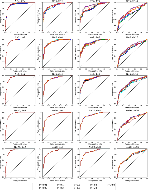
For $k\geq 1$, we apply the Adam optimizer (a variant of gradient descent), as implemented in PyTorch, to (9). In our experiments that follow, we use $N=10$ neurons and a few hundred iterations of Adam. On the other hand, for $k=0$, such a first-order scheme is not applicable due to the fact that the gradient of the $0^{\text{th}}$ degree ridge spline $(w^{\mathsf{T}}x-b)_{+}^{0}=1\{w^{\mathsf{T}}x\geq b\}$ (with respect to $w,b$) is almost everywhere zero. Therefore, as a surrogate, we instead approximate the optimum $w^{*},b^{*}$ in (2) using logistic regression. Appendix I provides further details on the optimization setup, and Appendices J and K present related sensitivity analyses.

4.2 Experimental setup

We compare the RKS tests of various degrees across several experimental settings, both to one another and to other all-purpose nonparametric tests: the energy distance test (Székely and Rizzo, 2005) as well as kernel MMD (Gretton et al., 2012) with a Gaussian kernel.

We fix the sample sizes to $m=n=512$ throughout, and consider four choices of dimension: $d=2,4,8,16$. For each dimension $d$, we consider five settings for $P,Q$, which are described in Table 1. In each setting, the parameter $v$ controls the discrepancy between $P$ and $Q$, but its precise meaning depends on the setting. The settings were broadly chosen in order to study the operating characteristics of the RKS test when differences between $P$ and $Q$ occur in one direction (settings 1–4), and in all directions (setting 5). Among the settings in which the differences occur in one direction, we also investigate different varieties (settings 1 and 2: mean shift under different geometries, setting 3: tail difference, setting 4: variance difference). Finally, we note that because the RKS test is rotationally invariant, the fact that the chosen differences in Table 1 are axis-aligned is just a matter of convenience, and the results would not change if these differences instead occurred along arbitrary directions in $\mathbb{R}^{d}$.

Setting	$P$	$Q$	$v$
Pancake mean shift (“pancake-shift”)	one axis $\sim{\mathcal{N}}(0,1)$ the others $\sim{\mathcal{N}}_{d-1}(0,16I)$	one axis $\sim{\mathcal{N}}(v,1)$ the others $\sim{\mathcal{N}}_{d-1}(0,16I)$	0.3
Ball mean shift (“ball-shift”)	${\mathcal{N}}_{d}(0,I)$	one axis $\sim{\mathcal{N}}(v,1)$ the others $\sim{\mathcal{N}}_{d-1}(0,I)$	0.2
$t$ coordinate (“t-coord”)	${\mathcal{N}}_{d}(0,I)$	one axis $\sim t(v)$ the others $\sim{\mathcal{N}}_{d-1}(0,I)$	3
Variance inflation in one direction (“var-one”)	${\mathcal{N}}_{d}(0,I)$	one axis $\sim{\mathcal{N}}(0,v)$ the others $\sim{\mathcal{N}}_{d-1}(0,I)$	1.4
Variance inflation in all directions (“var-all”)	${\mathcal{N}}_{d}(0,I)$	${\mathcal{N}}_{d}(0,vI)$	1.2

Table 1: Experimental settings. Here ${\mathcal{N}}(\mu,\Sigma)$ means the normal distribution with mean $\mu$ and covariance $\Sigma$, and $t(v)$ means the $t$ distribution with $v$ degrees of freedom.

For the RKS tests, we examine smoothness degrees $k=0,1,2,3$; for kernel MMD, we set the Gaussian kernel bandwidth according to a standard heuristic based on the median of all pairwise squared distances between the input samples (Caputo et al., 2002). (The energy distance test has no tuning parameters.) For each setting, we compute these test statistics under the null where each $x_{i}$ and $y_{i}$ are sampled i.i.d. from the mixture $\frac{m}{m+n}P+\frac{n}{m+n}Q$, and under the alternative where $x_{i}$ are i.i.d. from $P$ and $y_{i}$ from $Q$. We then repeat this 100 times (draws of samples, and computation of test statistics), and trace out ROC curves—true positive versus false positive rates—as we vary the rejection threshold for each test. Python code to replicate our experimental results is available at https://github.com/100shpaik/.

In Appendix L, we also compare the RKS test to kernel MMD with a polynomial kernel. Importantly, the latter is not actually a nonparametric test, for any finite polynomial order, since the population MMD does not define a metric (it cannot distinguish distributions $P,Q$ that agree up to some number of moments, interpreted in the multivariate sense, but differ otherwise). We include comparisons to polynomial kernels for completeness nonetheless.

4.3 Experimental results

Figure 2: ROC curves across the experimental settings described in Table 1. Each row represents a different setting, and each column a different dimension. The RKS, kernel MMD (KMMD), and energy distance tests are compared (each coded by a combination of color and line type).

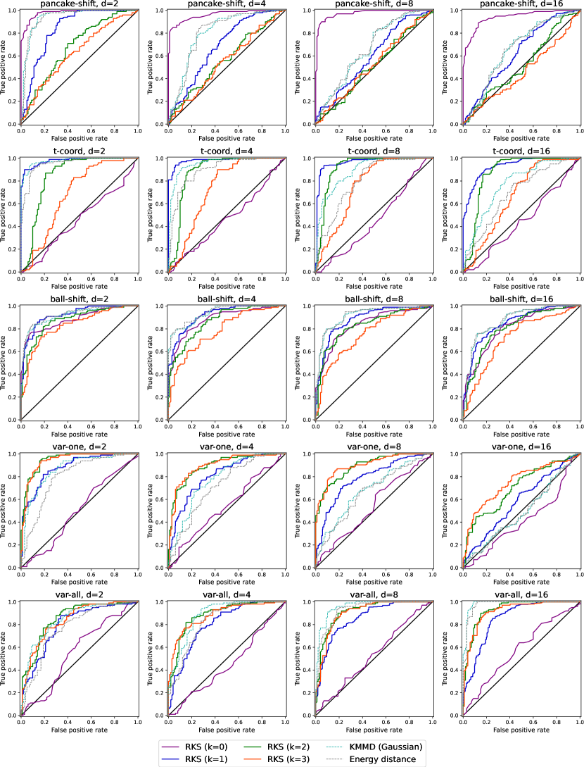
Figure 2 displays the ROC curves from all tests across all settings (rows) and all dimensions (columns). We see that in the first four settings (first four rows), the RKS tests exhibit generally strong performance: in each case, one of the $k^{\text{th}}$ degree RKS tests performs either the best or near-best among the methods considered. This supports the intuition discussed earlier, since in each of these settings, $P$ and $Q$ differ in only a small number (in fact, one) direction. Conversely, in the last setting, “var-all”, the distributions $P$ and $Q$ differ by a small amount in all directions, and the Gaussian kernel MMD and energy distance tests outperform the RKS tests, especially for larger $d$.

Keeping in mind that larger choices of $k$ correspond to higher-order truncated moments, we can further inspect the first four settings to try to learn from why the different order RKS tests perform better or worse. In the “pancake-shift” setting, the mean shift occurs in a low-variance direction, leading to nearly separable classes, so the smallest choice $k=0$ performs best, and better than kernel-based tests. In the “var-one” and “t-coord” settings, $P$ and $Q$ have the same mean, but different variance or tails, respectively, in one direction. Thus, larger choices of $k$ perform better: $k=1$ for “t-coord”, and $k=2,3$ for “var-one”. For a mean shift of between isotropic Gaussians, “ball-shift”, degrees $k=0,1,2$ are all reasonably competitive.

5 Discussion

We proposed and analyzed a new multivariate, nonparametric two-sample test, which is a maximum mean discrepancy (MMD) test with respect to a class of functions having unit Radon total variation, of a given smoothness degree $k\geq 0$. We call this the Radon-Kolmogorov-Smirnov (RKS) test, and it generalizes the well-known Kolmogorov-Smirnov (KS) test to multiple dimensions and higher orders of smoothness.

The RKS test, like any statistical test, is not expected to be most powerful in all scenarios. Roughly, we expect the RKS test to be favorable in settings in which the given distributions $P$ and $Q$ differ in only a few directions in the ambient space; and higher orders of smoothness $k$ can be more sensitive to tail differences along these few directions. When $P$ and $Q$ differ in many or all directions, the more traditional kernel MMD test with (say) Gaussian kernel will probably perform better.

It is worth revisiting computation of the RKS distance and discussing some limitations of our work and possible future directions. In this paper, we considered full batch gradient descent applied to (9) (we actually used Adam, but the differences for this discussion are unimportant), i.e., in each update the entire data set $\{x_{i}\}_{i=1}^{m}\cup\{y_{i}\}_{i=1}^{n}$ is used to calculate the gradient. This results in the following complexity: $T$ iterations of gradient descent costs $O((n+m)dNT)$ operations, where recall $N$ is the number of neurons. However, mini batch gradient descent should be also investigated, and is likely to be preferred in large problem sizes. That said, implementing mini batch gradients for (9) is nontrivial due to the nonseparable nature of the criterion across observations (due to the log and the absolute value in the first term), and pursuing this carefully is an important direction for future work. For now, we note that by just subsetting $P_{m},Q_{n}$ to a mini batch of size $b\leq n+m$, this results in a $T$ iteration complexity of $O(bdNT)$ operations. To compare kernel MMD: this costs $O((n+m)^{2}d)$ operations, and thus we can see that for large enough problem sizes computation of the RKS statistic via full batch and especially mini batch gradient descent can be more efficient, provided that small or moderate values of $N,T$ still suffice to obtain good performance.

Finally, another direction worth pursuing is the use of deeper networks, which could be interpreted as learning the feature representation in which there is the largest discrepancy in projected truncated moments. This would help further distinguish the RKS test from kernel MMD, because the latter is “stuck with” the representation provided by the choice of kernel, and it cannot learn the representation based on the data. A deep RKS test could dovetail nicely with existing architectures (and even pre-trained networks) for related tasks in areas such as generative modeling, and out-of-distribution detection.

Acknowledgments

We thank Rahul Parhi and Jonathan Siegel and helpful discussions about Radon bounded variation spaces. This work was supported by NSF SCALE MoDL grant 2134133, ONR MURI grant N00014-20-1-2787, and the Miller Institute for Basic Research in Science at the University of California, Berkeley.

Appendix A Proof of Proposition 1

By Theorem 22 in Parhi and Nowak (2021), every $\mathsf{f}\in{\mathrm{RBV}}^{k}$ has a representative $f\in\mathsf{f}$ of the form

$$f(x)=\int_{\mathbb{S}^{d-1}\times\mathbb{R}}\Big{[}(w^{\top}x-b)_{+}^{k}-\sum\nolimits_{|\alpha|\leq k}c_{\alpha}(w,b)x^{\alpha}\Big{]}\mathrm{d}\mu(w,b)+q_{0}(x),$$ (10)

for a finite Radon measure $\mu$ on ${\mathbb{S}^{d-1}\times\mathbb{R}}$ such that: (i) $\mu$ is an odd (respectively even) measure if $k$ is even (respectively odd); (ii) the integrand is integrable in $(w,b)$ with respect to $\mu$ for any $x$; (iii) $\|\mu\|_{{\rm TV}}=\|f\|_{{\mathrm{RTV}}^{k}}$; (iv) $q_{0}(x)$ is a polynomial of degree at most $k$; (v) $\sum_{|\alpha|\leq k}\big{(}c_{\alpha}(w,b)x^{\alpha}+(-1)^{k}c_{\alpha}(-w,-b)x^{\alpha}\big{)}=(w^{\mathsf{T}}x-b)^{k}$.

Using the conditions (i) and (v), we can show the following with a manual calculation and the change of variables $(w,b)\to(-w,-b)$:

$$\int_{\mathbb{S}^{d-1}\times(-\infty,0)}\Big{[}(w^{\top}x-b)_{+}^{k}-\sum\nolimits_{|\alpha|\leq k}c_{\alpha}(w,b)x^{\alpha}\Big{]}\;\mathrm{d}\mu(w,b)$$

$$=\int_{\mathbb{S}^{d-1}\times(0,\infty)}\Big{[}(-w^{\top}x+b)_{+}^{k}-\sum\nolimits_{|\alpha|\leq k}c_{\alpha}(-w,-b)x^{\alpha}\Big{]}\;\mathrm{d}\mu(-w,-b)$$

$$=\int_{\mathbb{S}^{d-1}\times(0,\infty)}(-1)^{2k+1}\Big{[}(w^{\top}x-b)_{-}^{k}-\sum\nolimits_{|\alpha|\leq k}(-1)^{k}c_{\alpha}(-w,-b)x^{\alpha}\Big{]}\;\mathrm{d}\mu(w,b)$$

$$=\int_{\mathbb{S}^{d-1}\times(0,\infty)}(-1)^{2k+1}\Big{[}(w^{\top}x-b)_{-}^{k}-(w^{\top}x-b)^{k}+\sum\nolimits_{|\alpha|\leq k}c_{\alpha}(w,b)x^{\alpha}\Big{]}\;\mathrm{d}\mu(w,b)$$

$$=\int_{\mathbb{S}^{d-1}\times(0,\infty)}\Big{[}(w^{\top}x-b)_{+}^{k}-\sum\nolimits_{|\alpha|\leq k}c_{\alpha}(w,b)x^{\alpha}\Big{]}\;\mathrm{d}\mu(w,b).$$ (11)

Define a measure $\tilde{\mu}$ by $\tilde{\mu}(E)=\mu(E_{0})+2\mu(E_{+})$ where for an event $E$ we denote $E_{0}=({\mathbb{S}^{d-1}\times\{0\}})\cap E$ and $E_{+}=({\mathbb{S}^{d-1}\times(0,\infty)})\cap E$. Then (A) rewrites (10) as

$$f(x)=\int_{\mathbb{S}^{d-1}\times[0,\infty)}\Big{[}(w^{\top}x-b)_{+}^{k}-\sum_{|\alpha|\leq k}c_{\alpha}(w,b)x^{\alpha}\Big{]}\;\mathrm{d}\tilde{\mu}(w,b)+q_{0}(x)$$ (12)

where $\|\tilde{\mu}\|_{\rm TV}=\|\mu\|_{\rm TV}=\|f\|_{{\mathrm{RTV}}^{k}}$. Note that $(w^{\top}x-b)_{+}^{k}$ is integrable in $(w,b)$ with respect to $\tilde{\mu}$ because $\|w\|_{2}=1$ and $b\geq 0$. Thus, $\int_{\mathbb{S}^{d-1}\times[0,\infty)}(w^{\mathsf{T}}x-b)_{+}^{k}\mathrm{d}\tilde{\mu}<\|x\|_{2}^{k}\|\tilde{\mu}\|_{\rm TV}$, hence $\sum_{|\alpha|\leq k}c_{\alpha}(w,b)x^{\alpha}$ is integrable with respect to $(w,b)$ for every $x$ as well. Thus,

$$q_{1}(x)=\int_{\mathbb{S}^{d-1}\times[0,\infty)}\Big{(}\sum\nolimits_{|\alpha|\leq k}c_{\alpha}(w,b)x^{\alpha}\Big{)}\mathrm{d}\tilde{\mu}(w,b)$$

is well-defined due to the condition (ii) and (12). Therefore (12) can be rewritten as

$$f(x)=\int_{\mathbb{S}^{d-1}\times[0,\infty)}(w^{\top}x-b)_{+}^{k}\;\mathrm{d}\tilde{\mu}(w,b)+\tilde{q_{0}}(x)$$

where $\tilde{q_{0}}(x)=q_{0}(x)+q_{1}(x)$ is a polynomial of degree at most $k$. Also $\tilde{\mu}|_{{\mathbb{S}^{d-1}\times\{0\}}}=\mu|_{{\mathbb{S}^{d-1}\times\{0\}}}$ by definition of $\tilde{\mu}$, and hence, $\tilde{\mu}|_{{\mathbb{S}^{d-1}\times\{0\}}}$ is odd when $k$ is even, and even when $k$ is odd by the condition (i). Thus, we have arrived at the desired representation.

Appendix B Proof of Theorem 1

We rely on the representation established by Proposition 1 and treat the cases $k=0$ and $k\geq 1$ separately.

Case $k=0$.

For this case, the boundary condition (continuity at the origin) implies that the integral may be restricted to $b>0$.

Lemma 1.

Consider $\mathsf{f}\in{\mathrm{RBV}}^{0}$. There exists a representative $f\in\mathsf{f}$ which is continuous at $0\in\mathbb{R}^{d}$ if and only if $f$ admits a representation

$$f(x)=\int_{{\mathbb{S}^{d-1}\times(0,\infty)}}1\{w^{\top}x\geq b\}\mathrm{d}\mu(w,b)+q,$$ (13)

where $q$ is a constant and $\mu$ is a signed measure with $\|\mu\|_{{\rm TV}}<\infty$.

Proof of Lemma 1.

By Proposition 1, there exists $f\in\mathsf{f}$ such that for all $x$,

$$f(x)=\int_{{\mathbb{S}^{d-1}\times[0,\infty)}}1\{w^{\top}x\geq b\}\mathrm{d}\mu(w,b)+q=f^{=0}(x)+f^{>0}(x),$$

where

$$\begin{gathered}f^{>0}(x)=\int_{{\mathbb{S}^{d-1}\times(0,\infty)}}1\{w^{\top}x\geq b\}\mathrm{d}\mu(w,b)+q,\\ f^{=0}(x)=\int_{{\mathbb{S}^{d-1}\times\{0\}}}1\{w^{\top}x\geq 0\}\mathrm{d}\mu(w,b).\end{gathered}$$

If $b>0$, then $\lim_{x\to 0}1\{w^{\top}x\geq b\}=0$. Thus, by dominated convergence,

$$\lim_{x\to 0}f^{>0}(x)=q(x)=f^{>0}(0).$$

Thus, $f^{>0}$ is continuous at $0$. We conclude that $f$ is almost-everywhere equal to a function which is continuous at 0 if and only if $f^{=0}$ is almost-everywhere equal to a function which is continuous at 0.

For $x\neq 0$, $w^{\top}x\geq 0$ if and only if $w^{\top}x/\|x\|\geq 0$. Thus, $f^{=0}(x)=f^{=0}(x/\|x\|)$. Thus, $f^{=0}$ is almost everywhere equal to a function which is continuous at $0$ if and only if there exists some $c\in\mathbb{R}$ such that for almost every $x\in\mathbb{S}^{d-1}$ (almost every with respect to Lebesgue surface measure), we have $f^{=0}(x)=c$. But this implies that $f^{=0}(x)=c$ for almost every $x\in\mathbb{R}^{d}$. Thus, we get that for almost every $x\in\mathbb{R}^{d}$,

$$f(x)=f^{>0}(x)+c=\int_{{\mathbb{S}^{d-1}\times(0,\infty)}}1\{w^{\top}x\geq b\}\mathrm{d}\mu(w,b)+q+c.$$

The right-hand side is the desired representative. ∎

Theorem 1 in the case $k=0$ is now a consequence of the following lemma, which additionally gives an explicit form for the radially cone continuous representative of $\mathsf{f}$.

Lemma 2.

Assume $\mathsf{f}\in{\mathrm{RBV}}^{0}$ contains a representative which is continuous at $0$. Then it contains a unique representative which is radially cone continuous. This representative can be written in the form (13) where $\mu$ is a signed measure with $\|\mu\|_{{\rm TV}}<\infty$. Conversely, any function of the form (13) where $\mu$ is a signed measure with $\|\mu\|_{{\rm TV}}<\infty$ is the unique radial cone continuous continuous representative of some $\mathsf{f}\in{\mathrm{RBV}}^{0}$.

Proof of Lemma 2.

Consider $\mathsf{f}\in{\mathrm{RBV}}^{0}$ which contains a representative which is continuous at the origin. By Lemma 1, there exists $f\in\mathsf{f}$ which satisfies (13) for all $x\in\mathbb{R}^{d}$, for some constant $q$ and signed measure $\mu$ with $\|\mu\|_{{\rm TV}}<\infty$.

Fix $x\neq 0$. Consider any sequence $\epsilon_{j}\in\mathbb{R}$ such that $\epsilon_{j}\downarrow 0$, and $v_{j}\in\mathbb{S}^{d-1}$ such that $v_{j}\to x/\|x\|$. Consider any $(w,b)\in{\mathbb{S}^{d-1}\times(0,\infty)}$. If $w^{\top}x<b$, then $w^{\top}(x+\epsilon_{j}v_{j})<b$ eventually because $x+\epsilon_{j}v_{j}\to x$. Alternatively, $w^{\top}x\geq b$ gives $w^{\top}x/\|x\|>0$, whence $w^{\top}v_{j}>0$ eventually. In particular, $w^{\top}(x+\epsilon_{j}v_{j})>w^{\top}x>0$ eventually. Thus, in both cases with have $1\{w^{\top}(x+\epsilon_{j}v_{j})\geq b\}\to 1\{w^{\top}x\geq b\}$. By dominated convergence, we get that

$$f(x+\epsilon_{j}v_{j}) =\int_{{\mathbb{S}^{d-1}\times(0,\infty)}}1\{w^{\top}(x+\epsilon_{j}v_{j})\geq b\}\mathrm{d}\mu(w,b)+q$$

$$\to\int_{{\mathbb{S}^{d-1}\times(0,\infty)}}1\{w^{\top}x\geq b\}\mathrm{d}\mu(w,b)+q=f(x).$$

Thus, $f$ is radially cone continuous and can be written in the form of (13).

By Theorem 22 in Parhi and Nowak (2021) and reversing the construction of $\tilde{\mu}$ from $\mu$ in the proof of Proposition 1, any function of the form (13) where $\mu$ is a signed measure with $\|\mu\|_{{\rm TV}}<\infty$ is a represenative of an equivalence class $\mathsf{f}\in{\mathrm{RBV}}^{0}$. The argument above also shows that it is radially cone continuous. Thus, we have shown the converse statement as well. ∎

Case $k=1$.

We begin with a lemma.

Lemma 3.

For $k\geq 1$ and every $\mathsf{f}\in{\mathrm{RBV}}^{k})$, there exists a unique representative $f\in\mathsf{f}$ which is continuous. This representative is in fact $(k-1)$-times continuously differentiable and can be written in the form in Proposition 1. Moreover, for any multi-index $\alpha$ with $|\alpha|\leq k-1$, we have for all $x\in\mathbb{R}^{d}$ that

$$D^{\alpha}f(x){}=\frac{k!}{(k-|\alpha|)!}\int_{{\mathbb{S}^{d-1}\times[0,\infty)}}w^{\alpha}(w^{\top}x-b)_{+}^{k-|\alpha|}\mathrm{d}\mu(w,b)+D^{\alpha}q(x).$$ (14)

where $w^{\alpha}=\prod_{i=1}^{d}w_{i}^{\alpha_{i}}$.

Proof of Lemma 3.

For any $\mathsf{f}\in{\mathrm{RBV}}^{k}$, let $f\in\mathsf{f}$ be a representative of the form in Proposition 1. We will show that this representative $f$ is $(k-1)$-times continuously differentiable by inducting on the order $m=|\alpha|$ of the multi-index $\alpha$.

The base case is $m=0$. In this case, the representation of the $0^{\text{th}}$ derivative is equivalent to the representation in the proposition. The continuity of $f$ follows by Lemma 9 applied to this representation.

Now consider $m\geq 1$, and assume we have established the result for $m-1$. Consider $\alpha$ with $|\alpha|=m$, and without loss of generality, assume $\alpha_{1}\geq 1$ and let $\tilde{\alpha}=(\alpha_{1}-1,\alpha_{2},\ldots,\alpha_{d})$. By the inductive hypothesis,

$$D^{\alpha}f(x)=\frac{k!}{(k-|\alpha|+1)!}\partial_{x_{1}}\int_{{\mathbb{S}^{d-1}\times[0,\infty)}}w^{\tilde{\alpha}}(w^{\top}x-b)_{+}^{k-|\alpha|+1}\mathrm{d}\mu(w,b)+D^{\alpha}q(x).$$

Note that for $x\in\mathbb{R}^{d}$, we have $\partial_{x_{1}}\big{(}w^{\tilde{\alpha}}(w^{\top}x-b)_{+}^{k-|\alpha|+1}\big{)}=(k-|\alpha|+1)w^{\alpha}(w^{\top}x-b)^{k-|\alpha|}$. This function is integrable in $(w,b)$ with respect to $\mu$ for every $x\in\mathbb{R}^{d}$, since $\|w\|_{2}=1$ and $b\geq 0$. Moreover, the partial derivative is uniformly bounded on $\{x^{\prime}:\|x^{\prime}\|\leq 2\|x\|\}$ by $2^{k-|\alpha|+1}(k-|\alpha|+1)\big{(}\prod_{i=1}^{d}|w_{i}|^{\alpha_{i}}\big{)}(2\|x\|)^{k-|\alpha|}$, which is integrable with respect to $\mu$. These conditions allow us to apply the Leibniz rule to conclude that we can exchange differentiation and integration, which yields (14). The continuity of $D^{\alpha}f$ then follows from Lemma 9, and hence, the induction is complete.

Thus we have shown that $f$ is $(k-1)$-times continuously differentiable. All that is left to show is that $f$ is the unique element of $\mathsf{f}$ which is $(k-1)$-times continuously differentiable. This holds because any two continuous functions which are equal almost everywhere are in fact equal everywhere. ∎

Theorem 1 in the case $k\geq 1$ is now a consequence of the following lemma, which additionally gives an explicit form for the radially cone continuous representative of $\mathsf{f}$.

Lemma 4.

For $k\geq 1$, let $\mathsf{f}\in{\mathrm{RBV}}^{k}$ be such that the unique continuous representative $f\in\mathsf{f}$ is $k$-times classically differentiable at $0\in\mathbb{R}^{d}$ with $D^{\alpha}f(0)=0$ for all $|\alpha|\leq k$. Then $f$ has representation of the form in Proposition 1 with $q(x)\equiv 0$.

Proof of Lemma 4.

Because $w^{\alpha}(w^{\top}0-b)_{+}^{k-|\alpha|}=0$ for $|\alpha|\leq k-1$ and any $(w,b)\in{\mathbb{S}^{d-1}\times[0,\infty)}$, (14) implies that $D^{\alpha}f(0)=D^{\alpha}q(0)$ for all $|\alpha|\leq k-1$.

Next, we evaluate $D^{\alpha}f(0)$ for $|\alpha|=k$, which, by assumption, exists. Without loss of generality, assume $\alpha_{1}\geq 1$, and let $\tilde{\alpha}=(\alpha_{1}-1,\alpha_{2},\ldots,\alpha_{d})$. Note that for $b>0$, $\partial_{x_{i}}w^{\tilde{\alpha}}(w^{\top}x-b)_{+}\big{|}_{x=0}=0$. By (14), we can write

$$D^{\alpha}f(0)=k!\partial_{x_{1}}\int_{{\mathbb{S}^{d-1}\times[0,\infty)}}w^{\tilde{\alpha}}(w^{\top}x-b)_{+}\;\mathrm{d}\mu(w,b)\Big{|}_{x=0}+D^{\alpha}q(0).$$

We compute the partial derivative in the first term manually:

$$\partial_{x_{1}}\int_{{\mathbb{S}^{d-1}\times[0,\infty)}}w^{\tilde{\alpha}}(w^{\top}x-b)_{+}\;\mathrm{d}\mu(w,b)\Big{|}_{x=0} =\lim_{h\to 0}\frac{1}{h}\int_{{\mathbb{S}^{d-1}\times[0,\infty)}}w^{\tilde{\alpha}}(w_{1}h-b)_{+}\;\mathrm{d}\mu(w,b).$$

For $b>0$ and $w\in\mathbb{S}^{d-1}$, we have $(w_{1}h-b)_{+}\leq|h|\cdot 1\{w_{1}h>b\}$ because $|w_{1}|\leq 1$. Also $|w^{\alpha}|\leq 1$ because $|w_{j}|\leq 1$ for all $j$. Thus,

$$\bigg{|}\frac{1}{h}\int_{\mathbb{S}^{d-1}\times(0,\infty)}w^{\tilde{\alpha}}(w_{1}h-b)_{+}\;\mathrm{d}\mu(w,b)\bigg{|} \leq\frac{1}{|h|}\int_{{\mathbb{S}^{d-1}\times(0,\infty)}}w^{\tilde{\alpha}}|h|1\{w_{j}h-b\}\;\mathrm{d}\mu(w,b)$$

$$\leq|\mu|\Big{(}(w,b)\in{\mathbb{S}^{d-1}\times(0,\infty)}:w_{j}h>b\Big{)}.$$

Because $|\mu|$ is a finite positive measure and $\bigcap_{h>0}\big{\{}(w,b)\in{\mathbb{S}^{d-1}\times(0,\infty)}:w_{j}h>b\big{\}}=\emptyset$, we conclude $|\mu|\big{(}(w,b)\in{\mathbb{S}^{d-1}\times(0,\infty)}:w_{j}h>b\big{)}\to 0$ as $h\to 0$. Thus, we have that

$$D^{\alpha}f(0)=k!\lim_{h\to 0}\Big{[}\frac{1}{h}\int_{{\mathbb{S}^{d-1}\times\{0\}}}w^{\tilde{\alpha}}(w_{1}h-b)_{+}\;\mathrm{d}\mu(w,b)\Big{]}+D^{\alpha}q(0),$$ (15)

and in particular, the limit in the first term exists. For $b=0$, $(w_{1}h-b)_{+}=w_{1}h\cdot 1\{w_{1}>0\}$ when $h>0$, and $(w_{1}h-b)_{+}=w_{1}h\cdot 1\{w_{1}<0\}$ when $h<0$. Thus, for $h>0$,

$$\frac{1}{h}\int_{{\mathbb{S}^{d-1}\times\{0\}}}w^{\tilde{\alpha}}(w_{1}h-b)_{+}\;\mathrm{d}\mu(w,b)=\int_{\begin{subarray}{c}{\mathbb{S}^{d-1}\times\{0\}}\\ w_{1}>0\end{subarray}}w^{\alpha}\;\mathrm{d}\mu(w,b),$$

and for $h<0$,

$$\frac{1}{h}\int_{{\mathbb{S}^{d-1}\times\{0\}}}w^{\tilde{\alpha}}(w_{1}h-b)_{+}\;\mathrm{d}\mu(w,b) =\int_{\begin{subarray}{c}{\mathbb{S}^{d-1}\times\{0\}}\\ w_{1}<0\end{subarray}}w^{\alpha}\;\mathrm{d}\mu(w,b)$$

$$=(-1)^{|\alpha|}(-1)^{k+1}\int_{\begin{subarray}{c}{\mathbb{S}^{d-1}\times\{0\}}\\ w_{1}>0\end{subarray}}w^{\alpha}\;\mathrm{d}\mu(w,b),$$

where the second equality uses the change of variables $w\mapsto-w$ and that $\mu|_{\mathbb{S}^{d-1}\times\{0\}}$ is odd when $k$ is even and even when $k$ is odd (see Proposition 1). By differentiability, the quantities in the two previous displays must be equal. Because $(-1)^{|\alpha|}(-1)^{k+1}=-1$, this implies that the quantities in the two previous displays must be 0. That is, the limit in (15) must be 0, and we have $0=D^{\alpha}f(0)=D^{\alpha}q(0)$.

We have thus shown that $D^{\alpha}q(0)=0$ for all $|\alpha|\leq k$, which, because $q(x)$ is a polynomial of degree at most $k$, implies $q(x)\equiv 0$. ∎

Appendix C Proof of Theorem 2

Theorem 2 is an immediate consequence of Lemmas 2 and 4.

Appendix D Proof of Theorem 3

We again treat the cases $k=0$ and $k\geq 1$ separately.

Case $k=0$.

Let

$${\mathcal{G}}_{0}^{+}=\Big{\{}1\{w^{\top}\cdot\geq b\}:\;(w,b)\in\mathbb{S}^{d-1}\times(0,\infty)\Big{\}}.$$

Because ${\mathcal{G}}_{0}^{+}\subseteq{\mathcal{G}}_{0}$, for any signed measure $\mu$ on ${\mathbb{S}^{d-1}\times(0,\infty)}$ with $\|\mu\|_{{\rm TV}}=1$ and $q\in\mathbb{R}$,

$$\sup_{f\in{\mathcal{G}}_{0}}P(f)-Q(f) \geq\sup_{f\in{\mathcal{G}}_{0}^{+}}P(f)-Q(f)\geq\int_{{\mathbb{S}^{d-1}\times(0,\infty)}}\int_{\mathbb{R}^{d}}1\{w^{\top}x\geq b\}\,\mathrm{d}(P-Q)(x)\,\mathrm{d}\mu(w,b)$$

$$=\int_{\mathbb{R}^{d}}\Big{(}\int_{\mathbb{S}^{d-1}\times(0,\infty)}1\{w^{\top}x\geq b\}\,\mathrm{d}\mu(w,b)+q\Big{)}\,\mathrm{d}(P-Q)(x).$$

Taking the supremum on the right-hand side over measure $\mu$, we get that

$$\sup\nolimits_{f\in{\mathcal{G}}_{0}}P(f)-Q(f)\geq\sup\nolimits_{f\in{\mathcal{F}}_{0}}P(f)-Q(f).$$

Because $\lim_{b\to\infty}P(w^{\top}x\geq b)-Q(w^{\top}x\geq b)$, $\mathbb{S}^{d-1}$ is compact, and $P(w^{\top}x\geq b)-Q(w^{\top}x\geq b)$ is continuous, the supremum on the left-hand side is achieved. Then, if the supremum is achieved at some $(w,b)$ with $b>0$, since $x\mapsto 1\{w^{\top}x\geq b\}\in{\mathcal{F}}_{0}$, we also have

$$\sup_{f\in{\mathcal{G}}_{0}}P(f)-Q(f)\leq\sup_{f\in{\mathcal{F}}_{0}}P(f)-Q(f).$$

On the other hand, consider that the supremum is achieved at some $(w,0)$. Note that

$$\lim_{b\uparrow 0}\;Q(w^{\top}x\leq b)-P(w^{\top}x\leq b)=P(w^{\top}x\geq 0)-Q(w^{\top}x\geq 0).$$

But $Q(w^{\top}x\leq b)-P(w^{\top}x\leq b)=P(f)_{b}-Q(f)_{b}$ for $f_{b}(x)=1\{-w^{\top}x\geq-b\}$. Note that $f_{b}\in{\mathcal{G}}_{0}^{+}$, and therefore, $f_{b}\in{\mathcal{F}}_{0}$. Thus, we have in this case also that $\sup_{f\in{\mathcal{G}}_{0}}P(f)-Q(f)\leq\sup_{f\in{\mathcal{F}}_{0}}P(f)-Q(f)$.

Having shown both directions of the inequality, we conclude $\sup_{f\in{\mathcal{G}}_{0}}P(f)-Q(f)=\sup_{f\in{\mathcal{F}}_{0}}P(f)-Q(f)$. The same result holds with the roles of $P$ and $Q$ reversed, which establishes the result with the supremum over $|P(f)-P(Q)|$.

Case $k\geq 1$.

Because $P$ and $Q$ have finite $k^{\text{th}}$ moments, by dominated convergence

$$(w,b)\mapsto\mathbb{E}_{P}[(w^{\top}x-b)_{+}^{k}]-\mathbb{E}_{Q}[(w^{\top}x-b)_{+}^{k}]$$

is continuous on ${\mathbb{S}^{d-1}\times[0,\infty)}$. Thus,

$$\sup_{f\in{\mathcal{G}}_{k}}P(f)-Q(f)=\sup_{(w,b)\in{\mathbb{S}^{d-1}\times(0,\infty)}}\mathbb{E}_{P}[(w^{\top}x-b)_{+}^{k}]-\mathbb{E}_{Q}[(w^{\top}x-b)_{+}^{k}]\leq\sup_{f\in{\mathcal{F}}_{k}}P(f)-Q(f),$$

where the last inequality holds because $x\mapsto(w^{\top}x-b)_{+}^{k}\in{\mathcal{F}}_{k}$ for all $w\in\mathbb{S}^{d-1}$ and $b>0$ (Parhi and Nowak, 2021). On the other hand, for any $f\in{\mathcal{F}}_{k}$,

$$P(f)-Q(f) =\int_{\mathbb{R}^{d}}\int_{\mathbb{S}^{d-1}\times[0,\infty)}(w^{\mathsf{T}}x-b)_{+}^{k}\,\mathrm{d}\mu(w,b)\,\mathrm{d}(P-Q)(x)$$

$$=\int_{\mathbb{S}^{d-1}\times[0,\infty)}\int_{\mathbb{R}^{d}}(w^{\mathsf{T}}x-b)_{+}^{k}\,\mathrm{d}(P-Q)(x)\,\mathrm{d}\mu(w,b)\leq\sup_{f^{\prime}\in{\mathcal{G}}_{k}}|P(f^{\prime})-Q(f^{\prime})|,$$

where the second equality uses Fubini’s theorem and the final inequality uses $\|\mu\|_{{\rm TV}}=\|\mathsf{f}\|_{{\mathrm{RTV}}^{k}}\leq 1$. Because the previous display holds for all $f\in{\mathcal{F}}_{k}$, we have $\sup_{f\in{\mathcal{F}}_{k}}P(f)-Q(f)=\sup_{f\in{\mathcal{G}}_{k}}|P(f)-Q(f)|$. Since $f\in{\mathcal{G}}_{k}$ implies $-f\in{\mathcal{G}}_{k}$, we have $\sup_{f\in{\mathcal{G}}_{k}}|P(f)-Q(f)|=\sup_{f\in{\mathcal{G}}_{k}}P(f)-Q(f)$.

Thus, we have shown both that $\sup_{f\in{\mathcal{G}}_{k}}|P(f)-Q(f)|\leq\sup_{f\in{\mathcal{F}}_{k}}|P(f)-Q(f)|$ and the reverse inequality, so that these are in fact equal.

Appendix E Proof of Theorem 4

If $P=Q$, then for any $f\in{\mathcal{F}}_{k}$, $P(f)-Q(f)=0$, whence $\rho(P,Q;{\mathcal{F}}_{k})=0$. Alternatively, consider $P\neq Q$. Then, by the uniqueness of the characteristic function, there exists $w\in\mathbb{R}^{d}$ such that the distribution of $w^{\top}X$ and $w^{\top}Y$, where $X\sim P$ and $Y\sim Q$, are different. This implies that there exists some $t\in\mathbb{R}$ such that $P(w^{\top}X\geq t)\neq Q(w^{\top}Y\geq t)$.

In what follows, we treat the cases $k=0$, $k=1$, and $k\geq 2$ separately.

Case $k=0$.

If $P(w^{\top}X\geq t)>Q(w^{\top}Y\geq t)$ for some $t\geq 0$, then taking $f(x)=1\{w^{\top}x\geq t\}$ gives

$$\rho(P,Q;{\mathcal{F}}_{0})=\rho(P,Q;{\mathcal{G}}_{0})\geq P(f)-Q(f)>0,$$

where we have used Theorem 3. If $P(w^{\top}X\geq t)>Q(w^{\top}Y\geq t)$ for some $t\leq 0$, then because $t\mapsto P(w^{\top}X\geq t)$ is left-continuous, for $s<t$ sufficiently close to $t$, we will have $P(w^{\top}X>s)>Q(w^{\top}Y>s)$. Then, taking $f(x)=-1\{(-w)^{\top}x\geq-s\}$ gives

$$\rho(P,Q;{\mathcal{F}}_{0})=\rho(P,Q;{\mathcal{G}}_{0})\geq P(f)-Q(f)>0,$$

where we have used Theorem 3.

Similarly, if $P(w^{\top}X\geq t)<Q(w^{\top}X\geq t)$, then we can take $f(x)=-1\{w^{\top}x\geq t\}$ in the case $t\geq 0$ and $f(x)=1\{(-w)^{\top}x\geq-s\}$ for some $s<t$ sufficiently close to $t$ to conclude $\rho(P,Q;{\mathcal{F}}_{0})>0$.

Case $k=1$.

Because $\mathbb{E}_{P}[1\{w^{\top}X\geq s\}]$ and $\mathbb{E}_{Q}[1\{w^{\top}Y\geq s\}]$ are left-continuous in $s$, if $w^{\top}X$ and $w^{\top}y$ have a different distribution, there is some open interval $(\alpha,\beta)\subseteq\mathbb{R}$ on which $\mathbb{E}_{P}[1\{w^{\top}X\geq s\}]>\mathbb{E}_{Q}[1\{w^{\top}Y\geq s\}]$ or $\mathbb{E}_{P}[1\{w^{\top}X\geq s\}]<\mathbb{E}_{Q}[1\{w^{\top}Y\geq s\}]$, uniformly over all $s\in(\alpha,\beta)$. Because either $\beta>0$ or $\alpha<0$, this interval contains an open interval entirely contained in either $\mathbb{R}_{>0}$ or $\mathbb{R}_{<0}$. In the former case, we have that for $b>0$, $\mathbb{E}_{P}[(w^{\top}X-b)_{+}]\neq\mathbb{E}_{Q}(w^{\top}Y-b)_{+}]$ because

$$\mathbb{E}_{P}\big{[}(w^{\top}X-b)_{+}\big{]}=\int_{b}^{\infty}\mathbb{E}_{P}\big{[}1\{w^{\top}X\geq s\}\big{]}\,\mathrm{d}s,\quad\mathbb{E}_{Q}\big{[}(w^{\top}Y-b)_{+}\big{]}=\int_{b}^{\infty}\mathbb{E}_{Q}\big{[}1\{w^{\top}Y\geq s\}\big{]}\,\mathrm{d}s.$$

We then get $\rho(P,Q;{\mathcal{F}}_{1})=\rho(P,Q;{\mathcal{G}}_{1})>0$ by taking $f(x)=(w^{\top}x-b)_{+}$. In the latter case, we have that for $b>0$, $\mathbb{E}_{P}[((-w)^{\top}X-b)_{+}]\neq\mathbb{E}_{Q}[((-w)^{\top}Y-b)_{+}]$ because

$$\mathbb{E}_{P}\big{[}((-w)^{\top}X-b)_{+}\big{]}=\int_{-\infty}^{-b}\mathbb{E}_{P}\big{[}(1-1\{w^{\top}X\geq s\})\big{]}\,\mathrm{d}s,$$

and likewise for $Q$. We then get $\rho(P,Q;{\mathcal{F}}_{1})=\rho(P,Q;{\mathcal{G}}_{1})>0$ by taking $f(x)=((-w)^{\top}x-b)_{+}$.

Case $k\geq 2$.

Note that the derivatives of the mappings $b\mapsto\mathbb{E}_{P}[(w^{\top}X-b)_{+}^{k}]$ and $b\mapsto\mathbb{E}_{Q}[(w^{\top}Y-b)_{+}^{k}]$ are $b\mapsto k\mathbb{E}_{P}[(w^{\top}X-b)_{+}^{k-1}]$ and $b\mapsto k\mathbb{E}_{Q}[(w^{\top}Y-b)_{+}^{k-1}]$, respectively. If there is some $(w,b)$ with $b\geq 0$ such that $\mathbb{E}_{P}[(w^{\top}X-b)_{+}^{k-1}]\neq\mathbb{E}_{P}[(w^{\top}X-b)_{+}^{k-1}]$, by continuity, $\mathbb{E}_{P}[(w^{\top}X-s)_{+}^{k-1}]\neq\mathbb{E}_{P}[(w^{\top}X-s)_{+}^{k-1}]$ for all $s$ in an open interval around $b$, whence, by integration, $\mathbb{E}_{P}[(w^{\top}X-s)_{+}^{k}]\neq\mathbb{E}_{P}[(w^{\top}X-s)_{+}^{k}]$ for some $s$ in this interval. We can then conclude the result by induction, using $k=1$ as a base case.

Appendix F Proof of Theorem 5

For a function class ${\mathcal{F}}$, a probability measure $\mathbb{P}$, and $\epsilon>0$, we say that $\{[l_{i},u_{i}]:i\in[N]\}$ is an $(\epsilon,\mathbb{P})$-bracket of ${\mathcal{F}}$ with cardinality $N$ if for all $i\in[N]$ we have $l_{i}(x)\leq u_{i}(x)$ for all $x$ and

$$\|u_{i}(X)-l_{i}(X)\|_{L^{2}(\mathbb{P})}^{2}=\mathbb{E}_{X\sim\mathbb{P}}[(u_{i}(X)-l_{i}(X))^{2}]\leq\epsilon^{2},$$

and for all $f\in{\mathcal{F}}$ there exists $i\in[N]$ such that $l_{i}(x)\leq f(x)\leq u_{i}(x)$ for all $x$. The $(\epsilon,\mathbb{P})$-bracketing number, which we denote by $N_{[\;]}(\epsilon;{\mathcal{F}},\|{\boldsymbol{\cdot}}\|_{L^{2}(\mathbb{P})})$, is the minimum cardinality of an $(\epsilon,\mathbb{P})$-bracket of ${\mathcal{F}}$. Using standard techniques from empirical process theory, we will be able to prove Theorem 5 by bounding the bracketing number $N_{[\;]}(\epsilon;{\mathcal{G}}_{k},\|{\boldsymbol{\cdot}}\|_{L^{2}(\mathbb{P})})$.

F.1 Bracketing number for ${\mathcal{G}}_{k}$ when $k\geq 1$

Theorem 7.

Let $k\geq 1$ and let $\mathbb{P}$ be a probability measure with finite $(2k+\Delta)$-moments for some $\Delta>0$, i.e., $\mathbb{E}_{X\sim\mathbb{P}}\|X\|_{2}^{2k+\Delta}=M<\infty$. Then, for the class ${\mathcal{G}}_{k}$, there is a constant $C_{[\;]}>0$ depending only on $M,d,\Delta$, and $k$ such that

$$\log N_{[\;]}(\epsilon;{\mathcal{G}}_{k},\|{\boldsymbol{\cdot}}\|_{2})\leq C_{[\;]}\log\Big{(}1+\frac{1}{\epsilon}\Big{)}.$$

Proof of Theorem 7.

We denote by ${\mathsf{B}}_{r}^{d}(x)$ the ball of radius $r$ centered at $x\in\mathbb{R}^{d}$:

$${\mathsf{B}}_{r}^{d}(x)=\{z\in\mathbb{R}^{d}\;|\;\|z-x\|_{2}^{2}\leq r^{2}\}.$$

We say a set $S\subseteq\mathbb{R}^{d}$ is a $r$-covering of a set $A\subseteq\mathbb{R}^{d}$ if $A$ is contained in the union of the balls of radius $\epsilon$ centered at points $x\in I$:

$$A\subseteq\bigcup\nolimits_{x\in I}{\mathsf{B}}_{r}^{d}(x).$$

For a compact set $I\subseteq\mathbb{R}^{d}$ and real number $b\in\mathbb{R}$, define functions

$$\ell_{I,b}(x) =\inf\Big{\{}(w^{\mathsf{T}}x-b)_{+}^{k}:w\in I\Big{\}},\quad\text{and}\quad u_{I,j}(x)=\sup\Big{\{}(w^{\mathsf{T}}x-b)_{+}^{k}:w\in I\Big{\}},$$

where we adopt the convention that $\ell_{I,\infty}(x)=u_{I,\infty}(x)\equiv 0$.

Lemma 5.

Consider $S$ is an $r$-covering of $\mathbb{S}^{d-1}$. Let $\mathcal{I}$ be the collection of sets $\{I=\mathbb{S}^{d-1}\cap{\mathsf{B}}_{r}^{d}(x):x\in S\}$, and let $b_{j}=j\delta$ for $j=-1,\ldots,N$, and $b_{N+1}=\infty$ for some $\delta>0$ and integer $N>0$. Then, the following is a bracket of ${\mathcal{G}}_{k}$

$$\big{\{}[l_{I,b_{j+1}},u_{I,b_{j}}]:I\in\mathcal{I},j=-1,\ldots,N\big{\}}.$$ (16)

Proof of Lemma 5.

Consider any $(w,b)\in{\mathbb{S}^{d-1}\times[0,\infty)}$ and its corresponding function $x\mapsto(w^{\mathsf{T}}x-b)_{+}^{k}\in{\mathcal{G}}_{k}$. Because $S$ is an $r$-covering, there exists $I\in\mathcal{I}$ such that $w\in I$. Also clearly there exists $j\in\{-1,0,1,\ldots,N\}$ such that $b_{j}<b\leq b_{j+1}$. Then $\ell_{I,j}\leq(w^{\mathsf{T}}x-b)_{+}^{k}$:

$$\ell_{I,b_{j}}(x)=\inf\Big{\{}(\tilde{w}^{\mathsf{T}}x-b_{j})_{+}^{k}:w\in I\Big{\}}\leq(w^{\mathsf{T}}x-b_{j+1})_{+}^{k}\leq(w^{\mathsf{T}}x-b)_{+}^{k}.$$

Similarly, we can show $(w^{\mathsf{T}}x-b)_{+}^{k}\leq u_{I,j}(x)$. ∎

Lemma 6.

In the setting of Lemma 5, if we set $r=\delta=\frac{\epsilon/3}{k\sqrt{1+\max(1,M)}}$ and $N=\lceil(\frac{M}{\epsilon})^{1/\Delta}\frac{1}{\delta}\rceil$, then we have $\|u_{I,b_{j}}-l_{I,b_{j+1}}\|_{L^{2}(P)}\leq\epsilon$ for all $j=-1,\ldots,N$ and $I\in\mathcal{I}$.

Proof of Lemma 6.

We bound

$$|u_{I,b_{j}}(x)-l_{I,b_{j+1}}(x)| \leq\max_{w,v\in I}|(w^{\mathsf{T}}x-b_{j})_{+}^{k}-(v^{\mathsf{T}}x-b_{j+1})_{+}^{k}|$$

$$\leq\max_{w,v\in I}|(w^{\mathsf{T}}x-b_{j})_{+}^{k}-(v^{\mathsf{T}}x-b_{j})_{+}^{k}|+\max_{v\in I}|(v^{\mathsf{T}}x-b_{j})_{+}^{k}-(v^{\mathsf{T}}x-b_{j+1})_{+}^{k}|.$$

Using a telescoping sum, we may bound for $j\leq N$

$$|(w^{\mathsf{T}}x-b_{j})_{+}^{k}-(v^{\mathsf{T}}x-b_{j})_{+}^{k}| =|(w^{\mathsf{T}}x-b_{j})_{+}-(v^{\mathsf{T}}x-b_{j})_{+}|\times\sum\nolimits_{i=0}^{k-1}(w^{\mathsf{T}}x-b_{j})_{+}^{i}(v^{\mathsf{T}}x-b_{j})_{+}^{k-1-i}$$

$$\leq\|w-v\|_{2}\|x\|_{2}\times k\cdot\max\{(w^{\mathsf{T}}x)_{+},(v^{T}x)_{+}\}^{k-1}$$

$$\leq k\|w-v\|_{2}\|x\|_{2}^{k}$$

$$\leq 2kr\|x\|_{2}^{k}.$$

Likewise, we may bound for $j\leq N-1$

$$|(v^{\mathsf{T}}x-b_{j})_{+}^{k}-(v^{\mathsf{T}}x-b_{j+1})_{+}^{k}| =|(v^{\mathsf{T}}x-b_{j})_{+}-(v^{\mathsf{T}}x-b_{j+1})_{+}|\times\sum\nolimits_{i=0}^{k-1}(v^{\mathsf{T}}x-b_{j})_{+}^{i}(v^{\mathsf{T}}x-b_{j+1})_{+}^{k-1-i}$$

$$\leq|b_{j}-b_{j+1}|\times k\cdot(v^{\mathsf{T}}x-b_{j})_{+}^{k-1-i}$$

$$\leq k\delta\|x\|_{2}^{k-1}.$$

Therefore, for $j\leq N-1$,

$$|u_{I,b_{j}}(x)-l_{I,b_{j+1}}(x)|\leq k\delta\|x\|_{2}^{k-1}+2kr\|x\|_{2}^{k}\leq\begin{cases}k(\delta+2r)&:\|x\|_{2}\leq 1\\ k(\delta+2r)\|x\|_{2}^{k}&:\|x\|_{2}>1\end{cases},$$

which can be simplified to

$$|u_{I,b_{j}}(x)-l_{I,b_{j+1}}(x)|\leq k(\delta+2r)\max\{1,\|x\|_{2}^{k}\}.$$

This gives for $j\leq N-1$,

$$\|u_{I,b_{j}}-l_{I,b_{j+1}}\|_{L^{2}(\mathbb{P})}^{2}\leq k^{2}(\delta+2r)^{2}(1+\mathbb{E}_{X\sim P}\|X\|_{2}^{2k})\leq k^{2}(\delta+2r)^{2}\cdot\max(1,M)\leq\epsilon^{2},$$

where the final inequality is obtained by plugging in the values of $r$ and $\delta$ specified in the statement of the lemma.

Meanwhile, for $j=N$, we have $b_{j+1}=\infty$, so that $l_{I,b_{j+1}}=0$. Also, $b_{j}=N\delta\geq(M/\epsilon)^{1/\Delta}$. Thus,

$$\|u_{I,b_{N}}-l_{I,b_{N+1}}\|_{L^{2}(\mathbb{P})}^{2} =\int_{\mathbb{R}^{d}}u_{I,b_{N}}(x)^{2}\mathrm{d}\mathbb{P}(x)$$

$$\leq\int_{\mathbb{R}^{d}}(\|x\|_{2}-b_{N})_{+}^{2k}\mathrm{d}\mathbb{P}(x)=\int_{\mathbb{R}^{d}}(\|x\|_{2}-N\delta)_{+}^{2k}\mathrm{d}\mathbb{P}(x)$$

$$\leq\Big{(}\int_{\mathbb{R}^{d}}(\|x\|_{2}-N\delta)^{2k+p}\mathrm{d}\mathbb{P}(x)\Big{)}^{\frac{2k}{2k+\Delta}}\Big{(}\int_{\mathbb{R}^{d}}1(\|x\|_{2}\geq N\delta)\;\mathrm{d}\mathbb{P}(x)\Big{)}^{\frac{\Delta}{2k+\Delta}}$$

$$=M^{\frac{2k}{2k+\Delta}}\times\mathbb{P}\Big{(}\|X\|_{2}\geq C\delta\Big{)}^{\frac{p}{2k+\Delta}}$$

$$\leq M^{\frac{2k}{2k+\Delta}}\times\Big{(}\frac{M}{(N\delta)^{2k+\Delta}}\Big{)}^{\frac{\Delta}{2k+\Delta}}=\frac{M}{(N\delta)^{\Delta}},$$

where the second inequality uses Hölder’s inequality, and the last inequality used Markov inequality. With the value of $\delta$ and $N$ specified by the lemma, we conclude $\|u_{I,b_{N}}-l_{I,b_{N+1}}\|_{L^{2}(\mathbb{P})}^{2}\leq\epsilon^{2}$. ∎

We can now complete the proof of Theorem 7. By Dumer (2007), there exists an $r$-covering of $\mathbb{S}^{d-1}$ with cardinality at most $(1+2/r)^{d}$. Thus, using the choices of $r,\delta$, and $N$ in Lemma 6 gives an $(\epsilon,\mathbb{P})$-bracket of ${\mathcal{G}}_{k}$ that has cardinality at most

$$\Big{(}1+\frac{2k\sqrt{1+\max(1,M)}}{\epsilon/3}\Big{)}^{d}\Big{(}\big{(}\frac{M}{\epsilon}\big{)}^{1/\Delta}\;\frac{k\sqrt{1+\max(1,M)}}{\epsilon/3}+1\Big{)}\leq C(1+1/\epsilon)^{d+1+1/\Delta}.$$

with some constant $C$. The proof is completed. ∎

F.2 Bracketing number for ${\mathcal{G}}_{0}$

Theorem 8.

Let $\mathbb{P}$ be a probability measure with finite $\Delta$-moments for some $\Delta>0$, i.e., $\mathbb{E}_{X\sim\mathbb{P}}\|X\|_{2}^{\Delta}=M<\infty$. Suppose additionally that $\mathbb{P}$ is absolutely continuous with respect to Lebesgue measure and has bounded density, i.e. $\sup_{x\in\mathbb{R}^{d}}|p(x)|\leq M_{\infty}<\infty$. hen, for the class ${\mathcal{G}}_{0}$, there is a constant $C_{[\;]}>0$ depending only on $M$, $M_{\infty}$, $d$, and $\Delta$ such that

$$\log N_{[\;]}(\epsilon;{\mathcal{G}}_{0},\|{\boldsymbol{\cdot}}\|_{2})\leq C_{[\;]}\log\Big{(}1+\frac{1}{\epsilon}\Big{)}.$$

Proof.

We adopt the same notation used in the proof of Theorem 7. The set (16) is a bracket of ${\mathcal{G}}_{0}$ by Lemma 5. Now we show that it is an $\epsilon$-bracket for appropriate choices of $r,\delta$, and $N$.

Select $I\in\mathcal{I},j=-1,\ldots,N-1$. There exists a $w_{0}\in I$ such that $\|w-w_{0}\|_{2}\leq r$ for all $w\in I$, since $S$ is an $r$-cover of $\mathbb{S}^{d-1}$. Consequently, for any $x\in\mathbb{R}^{d}$

$$\max_{w\in I}\;1(w^{\top}x\geq b_{j})\; \leq\;1(w_{0}^{\top}x\geq b_{j}-r\|x\|_{2}),$$

$$\min_{v\in I}\;1(v^{\top}x\geq b_{j+1})\; \geq\;1(w_{0}^{\top}x\geq r\|x\|_{2}+b_{j+1})$$

Notice that since $w_{0}\in\mathbb{S}^{d-1}$, the random variable $w_{0}^{\top}X\in\mathbb{R}$ has a probability density that is upper bounded by $M_{\infty}$. Therefore, for any $R>0$,

$$\|u_{I,b_{j}}-l_{I,b_{j}}\|_{L^{2}(\mathbb{P})}^{2} =\mathbb{P}\Bigl{(}\max_{w,v}\;\Bigl{|}1(w^{\top}x\geq b_{j})-\min_{v\in I}\;1(v^{\top}x\geq b_{j+1})\Bigr{|}\Bigr{)}$$

$$\leq\mathbb{P}\Big{(}w_{0}^{\top}X\in[b_{j}-r\|X\|_{2},b_{j+1}+r\|X\|_{2}]\Bigr{)}$$

$$\leq\mathbb{P}\Big{(}w_{0}^{\top}X\in[b_{j}-rR,b_{j+1}+rR]\Bigr{)}+\mathbb{P}\Bigl{(}\|X\|_{2}\geq R\Bigr{)}$$

$$\leq M_{\infty}\Bigl{(}\delta+2rR\Bigr{)}+\mathbb{P}\Bigl{(}\|X\|_{2}\geq R\Bigr{)}$$

$$\leq M_{\infty}\Bigl{(}\delta+2rR\Bigr{)}+\frac{M}{R^{\Delta}},$$

with the last line following from Markov’s inequality. Taking $R=(3M/\epsilon^{2})^{1/\Delta}$, $r=\frac{\epsilon^{2}}{6RM_{\infty}}=\frac{\epsilon^{2(1+1/\Delta)}}{6(3M)^{1/\Delta}M_{\infty}}$ and $\delta=\frac{\epsilon^{2}}{3M_{\infty}}$ makes the above upper bound equal to $\epsilon^{2}$.

On the other hand for $I\in\mathcal{I},j=N$, we have $l_{w,b_{N}+1}=0$, and

$$\|u_{I,b_{N}}-l_{I,b_{N+1}}\|_{P}^{2} =\mathbb{P}\Bigl{(}\max_{w\in I}w^{\top}X\geq b_{N}\Bigr{)}$$

$$\leq\mathbb{P}\Bigl{(}\|X\|_{2}\geq b_{N}\Bigr{)}$$

$$\leq\frac{M}{(N\delta)^{\Delta}}.$$

Taking $N=\frac{(M/\epsilon^{2})^{1/\Delta}}{\delta}$ makes this upper bound equal to $\epsilon^{2}$. So for these choices of $r,\delta$ and $N$ the bracket is an $\epsilon$-bracket.

Finally, arguing as in the proof of Theorem 7 we conclude that there exists an $\epsilon$-bracket of ${\mathcal{G}}_{0}$ with cardinality at most

$$N\times\Bigl{(}1+\frac{2}{r}\Bigr{)}^{d}\leq C(1+\frac{1}{\epsilon})^{2d(1+1/\Delta)+2(1+1/\Delta)}.$$

This completes the proof. ∎

F.3 Proof of Theorem 5

Theorem 5 is a consequence of the $(\epsilon,\mathbb{P})$-bracketing number bound of Theorem 7 (and when $k=0$, Theorem 8) and the following result from empirical process theory, which we copy for convenience.

Theorem 9 (Theorems 7.6 and 9.1 in Dudley (2014)).

Let $(\Omega,\Sigma,P)$ be a probability space and let ${\mathcal{F}}\subseteq{\mathcal{L}}^{2}(\Omega,\Sigma,P)$ be such that

$$J_{[\;]}({\mathcal{F}},\|{\boldsymbol{\cdot}}\|_{2})=\int_{0}^{1}\sqrt{\log N_{[\;]}(\epsilon;{\mathcal{F}},\|{\boldsymbol{\cdot}}\|_{L^{2}(P)})}\;\mathrm{d}\epsilon<\infty.$$

Then, under the $P$-null hypothesis, as $m,n\rightarrow\infty$,

$$\sqrt{\frac{1}{m}+\frac{1}{n}}\,(P_{m}-Q_{n})\overset{d}{\to}\mathbb{G}_{P},\;\;\text{and hence}\;\;\sqrt{\frac{1}{m}+\frac{1}{n}}\,\sup_{f\in{\mathcal{F}}}\big{|}P_{m}f-Q_{n}f\big{|}\overset{d}{\to}\sup_{f\in{\mathcal{F}}}|\mathbb{G}_{P}(f)|.$$

Theorem 9 implies Theorem 5 because $\int_{0}^{1}\sqrt{\log(1+1/\epsilon)}\,\mathrm{d}\epsilon<\infty$.

Appendix G Proof of Theorem 6

Our proof follows closely the proof of the analogous result for the univariate higher-order Kolmogorov-Smirnov test in Sadhanala et al. (2019). We begin by recalling the following lemma, which appears as Theorem 2.14.2 and 2.14.5 in van der Vaart and Wellner (1996), the statement of which we transcribe from Sadhanala et al. (2019).

Lemma 7.

Let ${\mathcal{F}}$ be a class of functions with an envelope function $F$; i.e., $f\leq F$ for all $f\in{\mathcal{F}}$. Define

$$W=\sqrt{n}\sup\nolimits_{f\in{\mathcal{F}}}|P_{n}f-Pf|,$$

and let $J=\int_{0}^{1}\sqrt{\log N_{[]}(\epsilon;{\mathcal{F}},\|\cdot\|_{L^{2}(P)})}\mathrm{d}\epsilon$. If for $p\geq 2$, $\|F\|_{L^{p}(P)}<\infty$, then for a universal constant $c_{1}>0$,

$$\mathbb{E}[|W|^{p}]^{1/p}\leq c_{1}\big{(}\|F\|_{L^{2}(P)}J+n^{-1/2+1/p}\|F\|_{L^{p}(P)}\big{)}.$$

If, for $0<p\leq 1$, the exponential Orlicz norm of $F$, i.e. $\|F\|_{\Psi_{p}}=\inf\{t>0:\mathbb{E}[\exp(|F|^{p}/t^{p})]\leq 2\}$, is finite, then

$$\|W\|_{\Psi_{p}}\leq c\big{(}\|F\|_{L^{2}(P)}J+n^{-1/2}(1+\log n)^{1/2}\|F\|_{\Psi_{p}}\big{)}.$$

Using this lemma, we have the following theorem on the concentration of the the RKS test statistic on its population value.

Theorem 10 (Two sided tail bound for $T_{d,k}$).

We have the following tail bounds.

1. Consider $k=0$. Assume $P$ and $Q$ have $\Delta^{\text{th}}$ moment bounded by $M$ for $M,\Delta>0$, which are absolutely continuous with respect to Lebesuge measure, and have densities bounded by $M_{\infty}$. Then, for some constant $c_{0}$ depending only on $M,\Delta,M_{\infty}$, and $d$,

   $$|T_{d,k}-\rho(P,Q;{\mathcal{F}}_{k})|\leq c_{0}(\log(1/\alpha))\Big{(}\frac{1}{\sqrt{m}}+\frac{1}{\sqrt{n}}\Big{)}.$$

2. Consider $k\geq 1$. Assume $P$ and $Q$ have finite $p^{\text{th}}$ moments bounded by $M$ for $p=2k+\Delta$ for $M,\Delta>0$, then there exists a constant $c_{0}$ depending only on $M,\Delta,k$, and $d$, such that

   $$|T_{d,k}-\rho(P,Q;{\mathcal{F}}_{k})|\leq\frac{c_{0}}{\alpha^{1/p}}\Big{(}\frac{1}{\sqrt{m}}+\frac{1}{\sqrt{n}}\Big{)}$$

   with probability at least $1-\alpha$. Assume, on the other hand, that $\|X\|$ and $\|Y\|$ have Orlicz norm of order $0<p\leq 1$ bounded by $M$ when $X\sim P$ and $Y\sim Q$. Then there exists a constant $c_{0}$ depending only on $M,p,k$, and $d$, such that

   $$|T_{d,k}-\rho(P,Q;{\mathcal{F}}_{k})|\leq c_{0}(\log(1/\alpha))^{1/p}\Big{(}\frac{1}{\sqrt{m}}+\frac{1}{\sqrt{n}}\Big{)}.$$

Proof of Theorem 10.

First consider $k\geq 1$. Note that a bound on any Orlicz-norm of order $0<p\leq q$ implies a bound on the $(2k+\Delta)^{\text{th}}$-moments of $P,Q$ for $\Delta=1$. Thus, assuming either the moment bound or the Orlicz norm bound, Theorem 7 implies $J=\int_{0}^{1}\sqrt{\log N_{[]}(\epsilon;{\mathcal{G}}_{k},\|\cdot\|_{L^{2}(P)})}$ has a finite upper bound depending only on the $(2k+\Delta)^{\text{th}}$-moments of $P$ and $Q$, $d$, $\Delta$, and $k$. Take $F(x)=\|x\|_{2}^{k}$. If we only assume a bound on the $(2k+\Delta)^{\text{th}}$ moments of $P$ and $Q$, then take $p=2k+\Delta\geq 2$. In this case, $n^{-1/2+1/p}\leq 1$, whence using Lemma 7 and Markov’s inequality, we see that $\sup_{f\in{\mathcal{F}}}|P_{n}f-Pf|\leq c_{0}/(\alpha^{1/p}\sqrt{n})$ and $\sup_{f\in{\mathcal{F}}}|Q_{n}f-Qf|\leq c_{0}/(\alpha^{1/p}\sqrt{m})$ with probability at least $1-\alpha$. The asserted bound then holds by the triangle inequality. On the other hand, if we assume a bound on the Orlicz norm of order $p$, Lemma 7 implies a constant upper bound on the Orlicz norm of order $p$ of $\sqrt{n}\sup_{f\in{\mathcal{F}}}|P_{n}f-Pf|$ and $\sqrt{m}\sup_{f\in{\mathcal{F}}}|Q_{n}f-Qf|$ because $(1+\log n)^{1/2}/n^{1/2}\leq 1$. This gives us the desired tail bound by taking $t=c_{0}(\log(1/\alpha))^{1/p}$ in the supremum defining the Orlicz norm and Markov’s inequality.

Now consider $k=0$. We take $F$ as a constant 1 function, i.e. $F=1$, and using Theorem 8 to bound the integral $J$ in this case. Because $F=1$ has a finite Orlicz norm of order $p=1$, the asserted tail bound follows from Lemma 7. ∎

We can now complete the proof of Theorem 6. By Theorem 5, if $P=Q$, then $T_{d,k}=O_{p}(\sqrt{(n+m)/(nm)}$. Because $1/t_{n+m}=o(\sqrt{n+m})=o(\sqrt{(nm)/(n+m)})$, we see that the test rejects with asymptotic probability 0. On the other hand, if $P\neq Q$, by Theorem 4, $\rho(P,Q;{\mathcal{F}}_{k})>0$. By Theorem 10, $T_{d,k}\stackrel{{\scriptstyle p}}{{\to}}\rho(P,Q;{\mathcal{F}}_{k})$. Because $t_{n+m}\to 0$, this implies that the test rejects with asymptotic probability 1. The proof is complete.

Appendix H Auxilliary technical lemmas

Lemma 8.

For $a,b\in\mathbb{R}$ and integer $k\geq 1$,

$$\big{|}a_{+}^{k}-b_{+}^{k}\big{|}\leq k(a_{+}^{k-1}+b_{+}^{k-1})|a-b|,$$

with the convention that when $k-1=0$, we set $0^{0}=1$.

Proof of Lemma 8.

Without loss of generality, assume $a\leq b$. The function $x\mapsto x_{+}^{k}$ has derivative $kx_{+}^{k-1}$ almost everywhere (even under our convention for when $k-1=0$). For every point $x\in[a,b]$, we have $|kx_{+}^{k-1}|\leq k(a_{+}^{k-1}+b_{+}^{k-1})$, because $|x_{+}|\leq\max\{a_{+},b_{+}\}$. Thus, integrating the derivative along the path between $a$ and $b$ gives the result. ∎

Lemma 9.

Assume $\mu\in{\mathcal{M}}({\mathbb{S}^{d-1}\times[0,\infty)})$. Then, for any $0\leq m\leq k-1$ and any function $c(w,b):{\mathbb{S}^{d-1}\times[0,\infty)}\rightarrow\mathbb{R}$ which is bounded by $|c(w,b)|\leq C$ for some constant $C$, we have

$$x\mapsto\int_{\mathbb{S}^{d-1}\times[0,\infty)}\Big{(}c(w,b)(w^{\mathsf{T}}x-b)_{+}^{k-m}\Big{)}\;\mathrm{d}\mu(w,b)$$ (17)

is continuous at every $x\in\mathbb{R}^{d}$.

Proof of Lemma 9.

Denote $f(x)=\int_{\mathbb{S}^{d-1}\times[0,\infty)}c(w,b)(w^{\mathsf{T}}x-b)_{+}^{k-m}\;\mathrm{d}\mu(w,b)$. Let $|\mu|$ be the total variation measure of the signed measure $\mu$. Note that $\|\mu\|_{\rm TV}=\|\,|\mu|\,\|_{\rm TV}$. For $x,y\in\mathbb{R}^{d}$,

$$\big{|}f (x)-f(y)\big{|}\leq\int_{\mathbb{S}^{d-1}\times[0,\infty)}|c(w,b)|\,\big{|}(w^{\top}x-b)_{+}^{k-m}-(w^{\top}y-b)_{+}^{k-m}\big{|}\;\mathrm{d}|\mu|(w,b)$$

$$\leq(k-m)\int_{\mathbb{S}^{d-1}\times[0,\infty)}|c(w,b)|\,\big{(}(w^{\top}x-b)_{+}^{k-m-1}+(w^{\top}y-b)_{+}^{k-m-1}\big{)}|w^{\top}(x-y)|\;\mathrm{d}|\mu|(w,b)$$

$$\leq(k-m)\|x-y\|\,\int_{\mathbb{S}^{d-1}\times[0,\infty)}|c(w,b)|\,\big{(}(\|w\|_{2}\|x\|_{2})^{k-m-1}+(\|w\|_{2}\|y\|_{2})^{k-m-1}\big{)}\;\mathrm{d}\mu(w,b)$$

$$\leq(k-m)\|x-y\|\,C\,\|\mu\|_{\rm TV}\,\big{(}\|x\|_{2}^{k-m-1}+\|y\|_{2}^{k-m-1}\big{)},$$

where in the second inequality we have used Lemma 8. Since the right-hand side goes to $0$ as $y\rightarrow x$, the proof is complete. ∎

Appendix I Computational and experimental details

I.1 Proof of the representation (5)

For $\|w\|_{2}=1$ and $b\in\mathbb{R}$, we have $\|(w^{\top}\cdot-\,b)_{+}^{k}\|_{{\mathrm{RTV}}^{k}}=1$ by Parhi and Nowak (2021). Then, for $w\in\mathbb{R}^{d}$ and $a\in\mathbb{R}$, by the $k^{\text{th}}$ order homogeneity of the ridge splines, $\|a(w^{\top}\cdot-\,b)_{+}^{k}\|_{{\mathrm{RTV}}^{k}}=|a|\|w\|_{2}^{k}$. Recalling the notation used in (4), and using that $\|\cdot\|_{\mathrm{RTV}}^{k}$ is a seminorm, the triangle inequality implies

$$\big{\|}f_{(a_{j},w_{j},b_{j})_{j=1}^{N}}\|_{{\mathrm{RTV}}^{k}}\leq\sum_{j=1}^{N}|a_{j}|\|w_{j}\|_{2}^{k}.$$

Thus, defining

$${\mathcal{F}}_{k,N}=\bigg{\{}f_{(a_{j},w_{j},b_{j})_{j=1}^{N}}\,:\,(a_{j},w_{j},b_{j})\in\mathbb{R}\times\mathbb{R}^{d}\times(0,\infty),\;\sum_{j=1}^{N}|a_{j}|\|w_{j}\|_{2}^{k}\leq 1\bigg{\}},$$

we have ${\mathcal{F}}_{k,N}\subseteq{\mathcal{F}}_{k}$. Defining also ${\mathcal{G}}_{k}^{+}=\{(w^{\mathsf{T}}\cdot-\,b)_{+}^{k}\,:\,(w,b)\in{\mathbb{S}^{d-1}\times(0,\infty)}\}$, we have ${\mathcal{G}}_{k}^{+}\subseteq{\mathcal{F}}_{k,N}$, so

$$\sup\nolimits_{f\in{\mathcal{G}}_{k}^{+}}\,|P(f)-Q(f)|\leq\sup\nolimits_{f\in{\mathcal{F}}_{k,N}}\,|P(f)-Q(f)|\leq\sup\nolimits_{f\in{\mathcal{F}}_{N}}\,|P(f)-Q(f)|.$$

The leftmost supremum is unchanged if we include the origin, i.e., take the suprermum over $f\in{\mathcal{G}}_{k}$, which precisely defines $T_{d,k}$. And by Theorem 3, this in turn is equal to $\sup_{f\in{\mathcal{F}}_{k}}|P(f)-Q(f)|$, the rightmost supremum above, so we conclude that all inequalities are equalities, and $T_{d,k}=\sup_{f\in{\mathcal{F}}_{k,N}}|P(f)-Q(f)|$. Finally, we can remove the absolute value sign in the criterion because ${\mathcal{F}}_{k,N}$ is symmetric ($f\in{\mathcal{F}}_{k,N}\iff-f\in{\mathcal{F}}_{k,N}$), which completes the proof of (5) as an equivalent representation.

I.2 Data preprocessing

Two steps of data preprocessing are conducted before the calculation of the RKS test statistic. First, the data is centered to have the sample mean zero jointly across both samples. That is, each $x_{i}$ is replaced by $x_{j}-\frac{1}{m+n}\big{(}\sum_{i=1}^{m}x_{i}+\sum_{i=1}^{n}y_{i}\big{)}$, and likewise for $y_{i}$. This makes the RKS test is translation-invariant. Second, after the centering, all the data is scaled to have its sample average $\ell_{2}$ norm of 1. That is, each $x_{i}$ is replaced by $x_{i}/\big{(}\frac{1}{m+n}\big{(}\sum_{i=1}^{m}\|x_{i}\|_{2}^{2}+\sum_{i=1}^{n}\|y_{i}\|_{2}^{2}\big{)}\big{)}^{1/2}$ and likewise for $y_{i}$. The scaling has no real effect on the test statistic and is done only for optimization purposes. We return the MMD on the unstandardized data, which we do by multiplying the MMD on the standardized data by the $k^{\text{th}}$ power of the scaling factor, $\big{(}\frac{1}{m+n}\big{(}\sum_{i=1}^{m}\|x_{i}\|_{2}^{2}+\sum_{i=1}^{n}\|y_{i}\|_{2}^{2}\big{)}\big{)}^{k/2}$.

I.3 Optimization details

For $k\geq 1$, we solve a rescaled version of (9) (where implicitly here $f=f_{(a_{j},w_{j},b_{j})_{j=1}^{N}}$, as in (4)):

$$\min_{(a_{j},w_{j},b_{j})\in\mathbb{R}\times\mathbb{R}^{d}\times[0,\infty)}\,-\frac{1}{k}\log\bigg{(}\frac{1}{N}\big{|}P_{m}(f)-Q_{n}(f)\big{|}\bigg{)}+\frac{\lambda}{kN}\sum_{i=1}^{N}|a_{i}|\|w_{i}\|_{2}^{k},$$ (18)

using the torch.optim.Adam optimizer with betas parameter $(0.9,0.99)$; learning rate equal to 0.5; number of iterations $T=200$; Lagrangian penalty parameter $\lambda=1$; and number of neurons $N=10$. To enforce the nonnegativity condition on $b$, in each update we project $b$ to $[0,\infty)$ after the gradient step. Rather than take the last iterate, we take the value of the parameters $(a_{j}^{t},w_{j}^{t},b_{j}^{t})_{j=1}^{N}$ across the iterations $t=1,\dots,T$ that give the maximal MMD value (after rescaling by the ${\mathrm{RTV}}^{k}$ seminorm of the iterate so that it lies in the unit ball). Further, we repeat this over three random initializations, and select the best iterate in terms of MMD value among these initializations to be the final output.

When $k=0$, due to the fact that gradients are almost every zero, as explained in Section 4, we instead use logistic regression, as implemented by sklearn.linear_model.LogisticRegression.

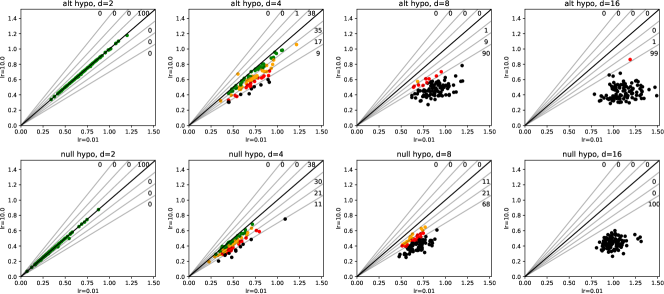
Appendix J Sensitivity analysis: log transform

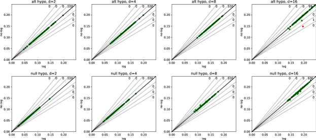
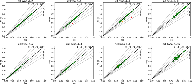
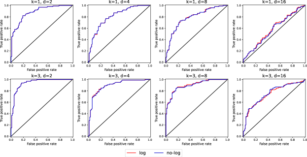
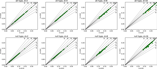
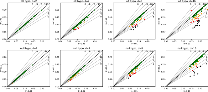
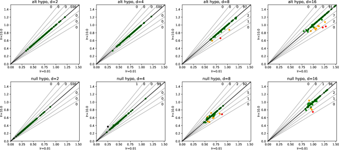
In (18), which is the basis for the experiments in the main paper, we use a log transform of the MMD term in the criterion. The current section compares the performance of (local) optimizers of this problem, which we call the “log” problem, for short, to those of

$$\min_{(a_{j},w_{j},b_{j})\in\mathbb{R}\times\mathbb{R}^{d}\times[0,\infty)}\,-\frac{1}{kN}\big{|}P_{m}(f)-Q_{n}(f)\big{|}+\frac{\lambda}{k}\bigg{(}\frac{1}{N}\sum_{i=1}^{N}|a_{i}|\|w_{i}\|_{2}^{k}\bigg{)}^{2},$$ (19)

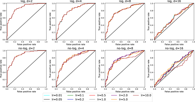
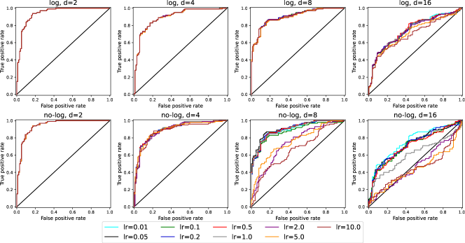
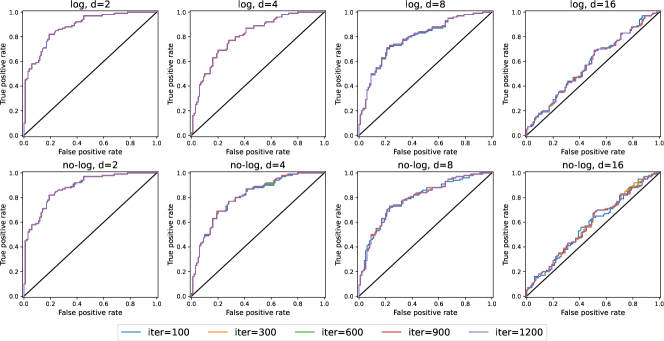
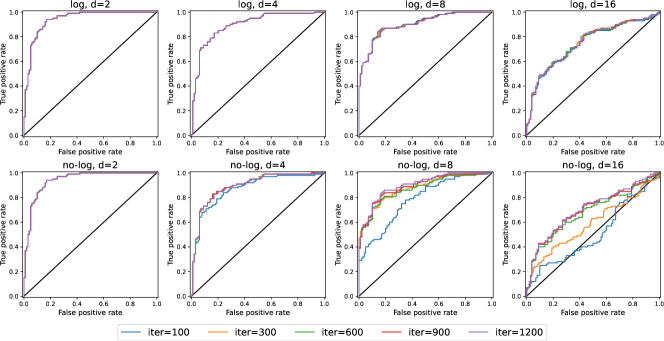
which we call the “no-log” problem, for short. In the above display, we can see that there is no log transform on the MMD term, but in addition, the penalty on the ${\mathrm{RTV}}^{k}$ seminorm has been squared. This is done because without such a transformation, one can show that the problem (MMD term plus ${\mathrm{RTV}}^{k}$ seminorm) does not attain its infimum, unless $\lambda$ is chosen very carefully so that the infimum in zero. By squaring the penalty, the criterion in (19) is coercive, which guarantees (since it is also continuous) that it will attain its infimum. In both (18) and (19), we fix $\lambda=1$, and use torch.optim.Adam with betas parameter $(0.9,0.99)$. We explore the behavior for different learning rates and numbers of iterations. Throughout, we focus on the “var-one” setting described in Table 1, and use $N=10$ neurons. The summary of our findings is as follows.

• Optimizing the “log” problem typically results in a larger MMD value compared to the “no-log” problem, especially for larger $k,d$, and especially under the null.

• Optimizing the “log” and “no-log” problems generally results in similar ROC curves, however, for larger $k,d$, the “no-log” ROC curves can actually be slightly better. This actually appears to be driven by the fact that “no-log” optimization is relatively worse in terms of the MMD values obtained under the null, which gives it a slightly greater separation and slightly higher power.

• The “log” problem is more robust to the choice of learning rate, both in terms of the MMD values and ROC curves obtained, especially for larger $k,d$.

• The “log” problem typically shows faster convergence (number of iterations required to approach a local optimum), especially for larger $k,d$.

Figures 4–9 display the results from our sensitivity analyses. In each one, the figure caption explains the salient points about the setup and takeaways. We remark that results for $k=4$ (not included for brevity) show qualitatively similar but even more extreme behavior.

(a) $k=1$

(b) $k=3$

Figure 3: MMD values obtained by optimizing the “log” (x-axis) and “no-log” (y-axis) problems. Each point represents a set of samples drawn from $P,Q$, and the result of running $T=1200$ iterations with learning rate $0.01$, for each criterion. (This learning rate was chosen to be favorable to the “no-log” problem.) Points below the diagonal mean that the “log” criterion results in a larger MMD value, which we see is especially prominent for larger $k,d$, and more prominent under the null.

Figure 4: ROC curves from the “log” and “no-log” problems, for the same data as in Figure 4. They are very similar except for the largest $k,d$ pair, where the “no-log” ROC curve is slightly better. Inspecting Figure 3(b), this is likely due to the fact that the null MMD values here are relatively smaller (poorer optimization).

(a) $k=1$, log

(b) $k=1$, no-log

Figure 5: MMD values corresponding to learning rates $0.01$ (x-axis) and $10$ (y-axis), for the same data as in Figure 4. There is little to no difference for the “log” problem (points near the diagonal), and a much bigger difference for the “no-log” problem, where in most cases the larger learning rate is worse (points below the diagonal).

(a) $k=3$, log

(b) $k=3$, no-log

Figure 6: MMD values corresponding to learning rates $0.01$ (x-axis) and $10$ (y-axis), for the same data as in Figure 4. There is little to moderate for the “log” problem (points around the diagonal), and a much bigger difference for the “no-log” problem, where in nearly all cases the larger learning rate is clearly much worse (points below the diagonal).

(a) $k=1$

(b) $k=3$

Figure 7: MMD values corresponding to learning rates from $0.01$ to $10$, for the same data as in Figure 4. In all cases, the “log” problem results in much more stable ROC curves with respect to the choice of learning rate, especially for larger $k,d$.

(a) $k=1$, $\text{lr}=0.01$

(b) $k=3$, $\text{lr}=0.01$

(c) $k=1$, $\text{lr}=0.5$

(d) $k=3$, $\text{lr}=0.5$

Figure 8: MMD value as a function of iteration for the “log” and “no-log” problems. This is done over 20 repetitions (draws of samples from $P,Q$); solid lines represent the median and shaded areas the interquartile range (computed over repetitions), at each iteration. For smaller $k,d$, the “log” and “no-log” convergence speeds are fairly similar, but for larger $k,d$, the “no-log” convergence speed is clearly slower. For the larger learning rate, we can also see that in many instances the “no-log” iterations fail to converge, and bounce up and down in MMD value, without staying at a local optimum.

(a) $k=1$

(b) $k=3$

Figure 9: ROC curves for the “log” and “no-log” problems, at different iteration numbers, over the same data in Figure 8. The “log” curves are quite robust to the choice of the number of iterations, whereas the “no-log” ones are not, especially for larger $k,d$. In other words, the “log” problem typically shows faster convergence (number of iterations required to approach a local optimum), especially for larger $k,d$.

Appendix K Sensitivity analysis: number of neurons

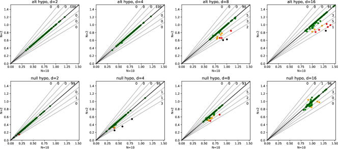
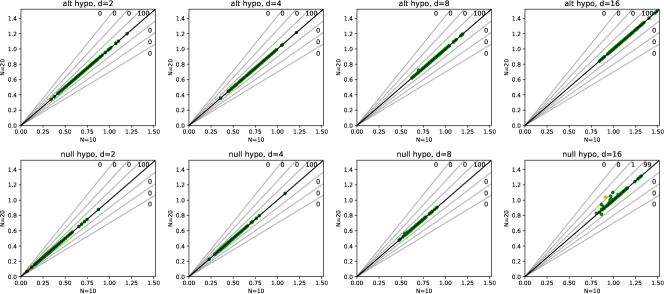
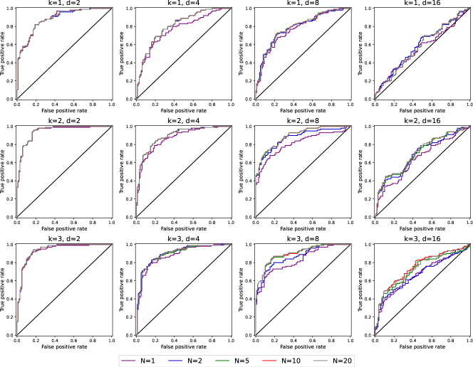
In this section, we now turn to investigate the role of the number of neurons $N$. We stick with the “log” problem (18) as in the experiments in the main text (with the previous section providing evidence that the log transform leads to greater robustness in many regards). The setup is essentially the same as that used in the last section, except that we vary the number of neurons from $N=1$ to $N=20$. The summary of our findings is as follows.

• Using a larger number of neurons often improves the achieved MMD value, especially for larger $k,d$; however, going past $N=10$ does not seem to make a big difference in our experiments.

• Using a larger number of neurons generally results in a better ROC curve, especially for larger $k,d$; again, going past $N=10$ does not seem to make a big difference in our experiments.

• Using a larger number of neurons can result in faster convergence, though not dramatically.

• Using a larger number of neurons is typically more robust to the choice of learning rate, both in terms of the MMD values and ROC curves obtained, especially for larger $k,d$.

Figure 11–14 display the results from our sensitivity analyses. As before, each figure caption presents the salient points about the setup and takeaways, and we remark that results for $k=4$ (not included for brevity) show qualitatively similar but even more extreme behavior.

Figure 10: MMD values when $N=10$ (x-axis) and $N=2$ (y-axis). Each point represents a set of samples drawn from $P,Q$, and the result of running $T=1200$ iterations with learning rate $0.5$, when $k=3$. Points below the diagonal mean that $N=10$ results in a larger MMD value, which we see is especially prominent for larger $k,d$, and more prominent under the null.

Figure 11: MMD values when $N=10$ (x-axis) and $N=20$ (y-axis). The setup is as above. Here we see no clear improvement in moving from $N=10$ to $N=20$ neurons.

Figure 12: ROC curves as the number of neurons varies from $N=1$ to $N=20$, for the same data as in Figure 11. The ROC curves look generally better for a larger number of neurons, especially for larger $k,d$.

(a) $k=1$, $\text{lr}=0.5$

(b) $k=3$, $\text{lr}=0.5$

Figure 13: MMD value as a function of iteration for $N=10$ and $N=2$ neurons. This is carried out over 20 repetitions (draws of samples from $P,Q$); solid lines represent the median and shaded areas the interquartile range (computed over repetitions), at each iteration. The convergence speed is sometimes slightly faster with $N=10$ neurons but the differences are not large.

Figure 14: ROC curves as the number of neurons varies from $N=1$ to $N=20$, and for varying learning rates, for the same data as in Figure 11. A larger number of neurons is typically more robust to the choice of learning rate, especially for larger $d$.

Appendix L Comparison to polynomial kernel MMD

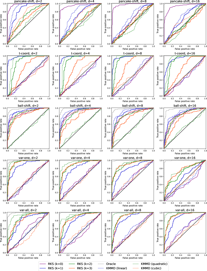
Figure 15 compares the RKS tests to the polynomial kernel MMD tests using the data as in Figure 2 in the main paper. We have chosen linear, quadratic, and cubic degree polynomials by (rough) analogy to the use of $k=1,2,3$ in RKS. The colors of the RKS test of degree $k$ and kernel MMD with a polynomial kernel of degree $k$ are chosen to match. However, we can see that these two frameworks produce tests with generally quite different behaviors: for example, compare the behavior of RKS with $k=1$ to kernel MMD with linear kernel, in the “t-coord” setting.

Altogether, the behavior of kernel MMD with polynomial kernel is as expected: it performs quite well when $P\neq Q$ differ according to the alternative (moment difference) that is anticipated by the test, and is otherwise essentially powerless.

Figure 15: ROC curves for the same data as in Figure 2, but now comparing RKS to kernel MMD (KMMD) with a polynomial kernel of linear, quadratic, and cubic degrees. The ROC curve from the likelihood ratio test is also shown, indicating the best possible performance for each setting (it depends on oracle knowledge of $P,Q$).

References

- Arjovsky et al. (2017) Martin Arjovsky, Soumith Chintala, and Léon Bottou. Wasserstein generative adversarial networks. In Proceedings of the International Conference on Machine Learning, 2017.
- Bach (2017) Francis Bach. Breaking the curse of dimensionality with convex neural networks. Journal of Machine Learning Research, 18(19):1–53, 2017.
- Baringhaus and Franz (2004) Ludwig Baringhaus and Carsten Franz. On a new multivariate two-sample test. Journal of Multivariate Analysis, 88(1):190–206, 2004.
- Bickel (1969) Peter J. Bickel. A distribution free version of the Smirnov two sample test in the p-variate case. Annals of Mathematical Statistics, 40(1):1–23, 1969.
- Bryson (1974) Maurice C. Bryson. Heavy-tailed distributions: Properties and tests. Technometrics, 16(1):61–68, 1974.
- Caputo et al. (2002) Barbara Caputo, K. Sim, Fredrik Furesjö, and Alexander J. Smola. Appearance-based object recognition using SVMs: Which kernel should i use? In Advances in Neural Information Processing Systems Workshop on Statistical Methods for Computational Experiments in Visual Processing and Computer Vision, 2002.
- Dudley (2014) Richard M. Dudley. Uniform Central Limit Theorems. Cambridge University Press, 2014. Second edition.
- Dumer (2007) Ilya Dumer. Covering spheres with spheres. Discrete & Computational Geometry, 38:665–679, 2007.
- Friedman and Rafsky (1979) Jerome H. Friedman and Lawrence C. Rafsky. Multivariate generalizations of the Wald-Wolfowitz and Smirnov two-sample tests. Annals of Statistics, 7(4):697–717, 1979.
- Goodfellow et al. (2014) Ian Goodfellow, Jean Pouget-Abadie, Mehdi Mirza, Bing Xu, David Warde-Farley, Sherjil Ozair, Aaron Courville, and Yoshua Bengio. Generative adversarial nets. In Advances in Neural Information Processing Systems, 2014.
- Gretton et al. (2012) Arthur Gretton, Karsten M. Borgwardt, Malte J. Rasch, Bernhard Schölkopf, and Alexander J. Smola. A kernel two-sample test. Journal of Machine Learning Research, 13:723–773, 2012.
- Henze (1988) Norbert Henze. A multivariate two-sample test based on the number of nearest neighbor type coincidences. Annals of Statistics, 16(2):772–783, 1988.
- Kolmogorov (1933) Andrey Kolmogorov. Sulla determinazione empirica di una legge di distribuzione. Giornale dell’Istituto Italiano degli Attuari, 4:83–91, 1933.
- Li et al. (2017) Chun-Liang Li, Wei-Cheng Chang, Yu Cheng, Yiming Yang, and Barnabás Póczos. MMD GAN: Towards deeper understanding of moment matching network. In Advances in Neural Information Processing Systems, 2017.
- Mroueh et al. (2018) Youssef Mroueh, Chun Liang Li, Tom Sercu, Anant Raj, and Yu Cheng. Sobolev gan. In Proceedings of the International Conference on Learning Representations, 2018.
- Müller (1997) Alfred Müller. Integral probability metrics and their generating classes of functions. Advances in Applied Probability, 29(2):429–443, 1997.
- Ongie et al. (2020) Greg Ongie, Rebecca Willett, Daniel Soudry, and Nathan Srebro. A function space view of bounded norm infinite width ReLU nets: The multivariate case. In Proceedings of the International Conference on Learning Representations, 2020.
- Parhi (2022) Rahul Parhi. On Ridge Splines, Neural Networks, and Variational Problems in Radon-Domain BV Spaces. PhD thesis, Department of Electrical and Computer Engineering, University of Wisconsin-Madison, 2022.
- Parhi and Nowak (2021) Rahul Parhi and Robert D. Nowak. Banach space representer theorems for neural networks and ridge splines. Journal of Machine Learning Research, 22(43):1–40, 2021.
- Parhi and Nowak (2023) Rahul Parhi and Robert D. Nowak. Near-minimax optimal estimation with shallow ReLU neural networks. Transactions on Information Theory, 69(2):1125–1140, 2023.
- Sadhanala et al. (2019) Veeranjaneyulu Sadhanala, Yu-Xiang Wang, Aaditya Ramdas, and Ryan J. Tibshirani. A higher-order Kolmogorov-Smirnov test. In Proceedings of the International Conference on Artificial Intelligence and Statistics, 2019.
- Savarese et al. (2019) Pedro Savarese, Itay Evron, Daniel Soudry, and Nathan Srebro. How do infinite width bounded norm networks look in function space? In Proceedings of the Annual Conference on Learning Theory, 2019.
- Schilling (1986) Mark F. Schilling. Multivariate two-sample tests based on nearest neighbors. Journal of the American Statistical Association, 81(395):799–806, 1986.
- Sejdinovic et al. (2013) Dino Sejdinovic, Bharath Sriperumbudur, Arthur Gretton, and Kenji Fukumizu. Equivalence of distance-based and RKHS-based statistics in hypothesis testing. Annals of Statistics, 41(5):2263–2291, 2013.
- Smirnov (1948) Nikolai Smirnov. Table for estimating the goodness of fit of empirical distributions. Annals of Mathematical Statistics, 19(2):279–281, 1948.
- Sriperumbudur et al. (2009) Bharath K. Sriperumbudur, Kenji Fukumizu, Arthur Gretton, Bernhard Scholkopf, and Gert R. G. Lanckriet. On integral probability metrics, -divergences and binary classification. arXiv preprint arXiv:0901.2698, 2009.
- Székely and Rizzo (2005) Gábor J. Székely and Maria L. Rizzo. A new test for multivariate normality. Journal of Multivariate Analysis, 93(1):58–80, 2005.
- van der Vaart and Wellner (1996) Aad van der Vaart and Jon Wellner. Weak Convergence and Empirical Processes: With Applications to Statistics. Springer, 1996.
- Wahba (1990) Grace Wahba. Spline Models for Observational Data. Society for Industrial and Applied Mathematics, 1990.
- Wang et al. (2014) Yu-Xiang Wang, Alexander J. Smola, and Ryan J. Tibshirani. The falling factorial basis and its statistical applications. In Proceedings of the International Conference on Machine Learning, 2014.