Primary and Secondary Order Parameters in the Fully Frustrated Transverse Field Ising Model on the Square Lattice

Abstract

Using quantum Monte Carlo simulations and field-theory arguments, we study the fully frustrated (Villain) transverse-field Ising model on the square lattice. We consider a “primary” spin order parameter and a “secondary” dimer order parameter, which both lead to the same phase diagram but detect $Z_{8}$ and $Z_{4}$ symmetry, respectively. The spin order scales with conventional exponents, both in the finite temperature critical phase and at the $T=0$ quantum critical point. The scaling of the dimer order requires more detailed investigations of the applicable low-energy theories; the height model at $T>0$ and the $O(2)$ model in 2+1 dimensions at $T=0$. Relating the order parameters to operators in these effective models, we predict the secondary critical exponents and confirm them numerically. The relationships between the primary and secondary order parameters have not been previously discussed in this context and provide insight more broadly for Ising models whose low-energy physics involves dimer degrees of freedom.

One of the simplest models exhibiting complex interplay of quantum and thermal fluctuations is the two-dimensional (2D) square-lattice fully frustrated transverse field Ising model (FFTFIM), with Hamiltonian

$$H=\sum_{\langle{ij}\rangle}J_{ij}\sigma_{i}^{z}\sigma_{j}^{z}-\Gamma\sum_{j}\sigma^{x}_{j},$$ (1)

where $\sigma_{i}^{x}$ and $\sigma_{i}^{z}$ are Pauli operators. The couplings $J_{ij}$ are equal in magnitude but the number of antiferromagnetic (AF) couplings around any elementary plaquette is odd (Villain’s odd model Villain (1977a)). To achieve this, we choose a gauge with $J_{ij}=+J$ (AF) on every second column and $J_{ij}=-J$ on all other bonds, as depicted in Fig. 1. It is impossible to satisfy all bonds on an elementary plaquette and the classical model at $\Gamma=0$ hosts a large ground state degeneracy that is lifted by the transverse field via an “order-by-disorder” mechanism Villain, J. et al. (1980); Moessner (2001); Henley (1989).

The FFTFIM was previously studied at temperature $T=0$ both semiclassically Coletta et al. (2014) and using quantum Monte Carlo (QMC) simulations Wenzel et al. (2012), where spin and dimer order was found for $\Gamma<\Gamma_{c}\sim 1.578$. In this phase the frustrated bonds (mapped to dimers as in Fig. 1) align along either columns or rows and can be characterized by a four-fold degeneracy and $Z_{4}$ breaking.

QMC simulations of the system at $T>0$ were carried out in the context of an effective quantum dimer model, which corresponds, for for the purely kinetic model, to the $\Gamma\to 0$ limit of the FFTFIM Dabholkar et al. (2022). At finite $\Gamma$, a theoretical study predicted that the $Z_{4}$-breaking and high-temperature paramagnet are separated by a critical phase bordered by two Kosterlitz-Thouless (KT) transitions Korshunov (2012). The stacked version of the classical model (i.e., in 2+1 dimensions, corresponding to $\Gamma>0$) has also been studied using Landau-Ginsburg-Wilson (LGW) theory, where an effective Hamiltonian suggested a $Z_{8}$ breaking ordered phase Blankschtein et al. (1984a). The reconciliation of $Z_{8}$ versus $Z_{4}$ breaking was touched on by Coletta et al. Coletta et al. (2014), but the relationship between the order parameters was not explored.

Figure 1: The degenerate classical ground states represented by elementary plaquettes. Blue and red bonds show $J_{ij}=-J$ and $J_{ij}=+J$, respectively. Sublattice magnetizations $m_{s}$, $s=1,\ldots,4$, are indicated by the arrows, and dimers (green ovals) are defined on the frustrated bonds. The values of the magnetization and dimer order parameters are indicated in each case [see Eqs. (3) and (5)].

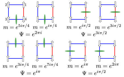
Here we define a proper $Z_{8}$ symmetric spin order parameter and demonstrate that the $Z_{4}$ dimer order parameter should be considered as secondary. While both order parameters lead to the same phase diagram (provided in Supplemental Material, Sec. SI sup ), the $Z_{4}$ order parameter exhibits faster decaying critical correlations. Both order parameters, when correctly defined, exhibit emergent $U(1)$ symmetry in the critical phase. We explain the secondary nature of the dimer order quantitatively by referencing the relevant field theories in the two temperature regimes, $T=0$ and $T>0$, and provide finite-size scaling of QMC (stochastic series expansion Sandvik (2003)) results of the full FFTFIM Hamiltonian, Eq. (1), to support the predicted scaling.

Secondary order parameters have previously been used to describe higher harmonic contributions to spatial modulation in density wave systems, e.g., liquid crystals Wu et al. (1994); Aharony et al. (1995); Hasenbusch and Vicari (2011); Netz and Aharony (1997); Calabrese and Parruccini (2005). A secondary order parameter can clearly be defined also in the FFTFIM, given the emergent $U(1)$ symmetry (stemming from the irrelevance of the discrete symmetry-breaking terms at criticality, as in 3D classical clock models José et al. (1977)). However, the different scaling forms of the spin and dimer order parameter in the FFTFIM have not been addressed. This Letter provides a framework for secondary order not just in the FFTFIM, but in the entire class of frustrated Ising models with effective dimer degrees of freedom, e.g., the antiferromagnet on the triangular lattice Blankschtein et al. (1984b); Blöte and Nightingale (1993); Isakov and Moessner (2003); Moessner and Sondhi (2001); Stephenson (2003).

Order Parameters.—To construct a proper primary order parameter, we follow the procedure by Isakov and Moessner in their study of the triangular AF model Isakov and Moessner (2003). We begin by referencing the analysis by Blankschtein et al. on Blankschtein et al. (1984a) a stacked classical model, where an effective Hamiltonian was constructed in terms of the amplitude $m$ and phase $\theta$ of critical modes:

$$\begin{split}H_{\rm eff}=\sum_{\vec{q}}(r+q^{2})|m|^{2}+u_{4}|m|^{4}+u_{6}|m|^{6}+\\ (u_{8}+v_{8}/32)|m|^{8}-(v_{8}/32)|m|^{8}\cos(8\theta).\end{split}$$ (2)

The eight-state clock anisotropy implies an eight-fold degenerate ground state, characterized by sublattice magnetizations $(m_{1},m_{2},m_{3},m_{4})$; see Fig. 1. Each state corresponds to one frustrated bond in a plaquette, with an overall spin-flip transformation giving a total of eight degenerate states. Blankschtein et al. (1984a); Coletta et al. (2014).

Based on the low-energy behavior of the stacked model, as well as the semiclassical analysis of Ref. Coletta et al. (2014), we define the primary order parameter as the complex number

$$\begin{split}m=&\,m_{x}+im_{y}=\\ &\frac{1}{2}\left(m_{1}e^{i\frac{\pi}{8}}+m_{2}e^{i\frac{3\pi}{8}}+m_{3}e^{i\frac{5\pi}{8}}+m_{4}e^{i\frac{7\pi}{8}}\right)\end{split}$$ (3)

where

$$m_{s}=\frac{4}{N}\sum_{j\in s}\sigma_{j}^{z}.$$ (4)

The eight ground state configurations of the stacked model correspond to $m=e^{in\pi/4}$, $n=1,2,\dots,8$.

The problem can also be mapped onto that of dimer coverings, where a dimer is assigned across each frustrated bond Moessner and Sondhi (2001), and we define a secondary order parameter $\Psi$ with this mapping in mind. This order parameter is also complex number, defined in terms of the dimer density modulation on the dual lattice Wenzel et al. (2012):

$$\Psi=\Psi_{x}+i\Psi_{y}=2\tilde{d}_{x}(0,\pi)+2i\tilde{d}_{y}(\pi,0),$$ (5)

where

$$\tilde{d}_{\alpha}(\boldsymbol{q})=\frac{1}{N}\sum_{i}e^{i\boldsymbol{q}\cdot\boldsymbol{r}_{i}}d_{i,\alpha},$$ (6)

is the Fourier transformed dimer density

$$d_{i,\alpha}=\frac{1}{2}\left(1+\frac{J_{i,j_{\alpha}}}{J}\sigma_{i}^{z}\sigma_{j_{\alpha}}^{z}\right),$$ (7)

and $j_{\alpha}$ is the index of nearest neighbor to site $i$ in the $\alpha$ direction. Long-range ordering is associated with $|\Psi|$ taking a finite value, while the specific (symmetry-broken) ordering pattern is identified by the phase. Thus, $\Psi$ takes one out of the values $e^{in\pi/2}$, $n=1,2,\dots,4$. The connection between the columnar states and the sublattice magnetizations is illustrated in Fig. 1.

$Z_{8}$ versus $Z_{4}$ Symmetry Breaking.—We detect the order-parameter symmetries by plotting the probability distributions of $m$ and $\Psi$ accumulated during QMC simulations. In the ordered phase, we expect eight (four) $\delta$-functions at the eight (four) values corresponding to the columnar spin (dimer) states in Fig. 1. These $\delta$-functions smear for finite systems, appearing as highly peaked Gaussian distributions for large systems.

In the critical phase, we observe the emergent $U(1)$ symmetry expected from the mapping to the height model Jiang and Emig (2005); Korshunov (2012); Henley (1997). We assign height differences to neighboring spins based whether or not the bond they share is frustrated (i.e., crossing a dimer) Korshunov (2012), as detailed in Supplemental Material, Sec. SII sup . In the ordered phase, the height profile is “flat,” with the height values bounded from above. In the critical and disordered phases, the model is in its “rough” phase, with a logarithmically diverging height profile. This behavior can be described by an effective elastic free energy with a periodic “locking” potential favoring the eight flat height configurations, i.e., the columnar states in Fig. 1. This effective free energy is precisely that of the 2D $XY$ model, where the locking potential corresponds to an $q=8$ state clock anisotropy term. This connection allowing us to apply the renormalization group (RG) analysis of Ref. José et al. (1977) to understand the observed behavior.

Jose et al. José et al. (1977) first showed that the classical 2D $q$-state clock model is characterized by three temperature regimes if $q>4$. At temperatures below the lower critical temperature $T_{\rm c1}$, the clock term is relevant and the system orders into the $Z_{q}$ clock phase. At $T$ above $T_{\rm c1}$ but below the upper critical temperature $T_{\rm c2}$, the clock term is irrelevant and the free energy reduces to that of the $XY$ model in the KT phase. In this phase, the system can freely fluctuate between the flat height configurations, thus resulting in the $U(1)$ symmetric distributions that we observe. Finally, above $T_{\rm c2}$ the critical phase melts into the disordered phase as defects proliferate.

Figure 2: Distributions of $(\Psi_{x},\Psi_{y})$ in (a,c) and $(m_{x},m_{y})$ in (b,d), collected in several independent simulations (each initialized in one of the four columnar states, to prevent trapping in states with topological defects) and symmetrized using lattice rotations and reflections. The system size is $L=96$ and $\Gamma/J=0.43$, with $T/J=0.21$ in (a,b) (in the critical phase) and $T/J=0.014$ in (c,d) (in the ordered phase).

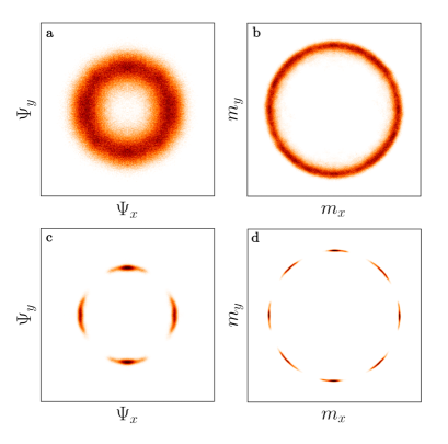
An example of the symmetry reduction in the ordered phase is shown in Fig. 2, where (a) and (b) are collected from simulations in the critical phase, while (c) and (d) are from the ordered phase. While we detect emergent $U(1)$ symmetry in both order parameters, a $U(1)$ phase would not be expected for a primary $Z_{4}$ dimer order parameter at $T>0$, given the $q>4$ criterion in the clock model José et al. (1977). However, with the spin order parameter corresponding to $q=8$, the critical phase is expected.

Scaling at $T>0$.—As a quantitative characterization of the primary and secondary natures of the two order parameters, we compare the scaling of their respective correlation functions in the critical phase. Within the $q$-state clock-model description, the spin-spin correlations should decay algebraically with a scaling exponent $\eta$ that varies continuously with the temperature Nienhuis et al. (1984). The value of $\eta$ at the upper and lower critical temperatures are known, $\eta=1/4$ and $\eta=4/q^{2}$, respectively José et al. (1977); Henley (1997). To extract $\eta$, we examine the magnitudes of both order parameters, which in this phase should scale with the lattice length $L$ as

$$|m|^{2}\propto L^{-\eta_{m}},~{}~{}~{}~{}|\Psi|^{2}\propto L^{-\eta_{d}},$$ (8)

where we leave open the possibility that $\eta_{m}\neq\eta_{d}$. In Fig. 3(a) and 3(b), the order parameters are plotted versus system size for a range of temperatures between $T_{\rm c1}$ and $T_{\rm c2}$. As predicted, they scale algebraically with $L$, and we extract $\eta_{m}(T)$ and $\eta_{d}(T)$ by fitting data to Eq. (8). Results are shown versus $T$ in Fig. 3(c).

Figure 3: Log-log plots of the magnitude of the primary (a) and secondary (b) order parameter versus the system size $L$ for a range of temperatures at $\Gamma/J=0.67$. The dashed lines are power-law fits to the largest eight system sizes, with $T$ increasing with color brightness (red to orange). (c) Anomalous dimensions $\eta_{m,d}$ versus $T$ for the primary (red) and secondary (blue) order parameters, extracted from fitting data to Eq. (8). The exponents align if $\eta_{d}$ is rescaled by a factor $1/4$. The gray box denotes $T_{\rm c2}\pm\sigma$ from Binder crossing results. The dashed lines are at the predicted values at the phase boundaries.

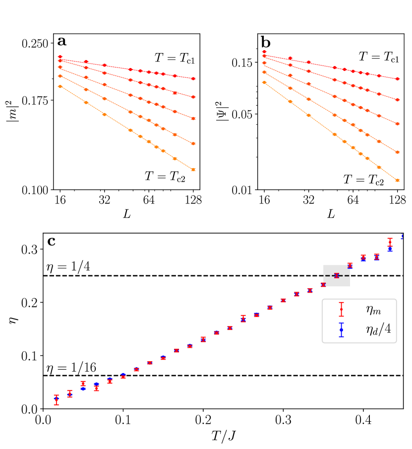
The primary order parameter scales with the expected exponent $\eta_{m}=1/4$ at the upper critical temperature $T_{\rm c2}$ extracted from Binder crossing results (Supplemental Information, Sec. SI sup ). Below this temperature, the exponent linearly decreases. The statistical quality of the fits deteriorates below the temperature at which $\eta_{m}=1/16$ (see Supplemental Material, Sec. SIII sup ), which is the predicted value at the lower transition point $T_{\rm c1}$ José et al. (1977), where the system orders. Thus, our numerical results are consistent with the theory, and we can use $\eta_{m}=1/4$ and $\eta_{m}=1/16$ to set more precise upper and lower boundaries.

The same behavior is observed for the dimer order parameter, except that the value of the $\eta_{d}$ is consistently approximately four times larger than $\eta_{m}$. After rescaling $\eta_{d}$ by a factor of four, the results match within statistical errors, suggesting the relation $\eta_{d}=4\eta_{m}$. This relationship between $\eta_{m}$ and $\eta_{d}$ can be explained by the height model: the dimer value $d(\vec{r})$ at $\vec{r}$, is related to the product of neighboring spin operators, Eq. (7), which in the coarse-grained model can be considered simply as the square of the spin operator at $\vec{r}$, $\left(\sigma^{z}(\vec{r})\right)^{2}$. By representing the spin operators in terms of the height variables, one can relate the spin-spin and dimer-dimer correlation functions to the logarithmically diverging height difference profile; the observed factor of four relating $\eta_{d}$ and $\eta_{m}$ then emerges. For details, see Supplemental Material, Sec. SII sup .

Scaling at $T=0$.—At the quantum critical point, there must be a different relationship between $\eta_{d}$ and $\eta_{m}$. Given the irrelevance in 2+1 dimensions of $Z_{4}$ or $Z_{8}$ perturbations to a $U(1)$ order parameter, the primary order parameter should scale with the conventional 3D $XY$ critical exponent $1+\eta_{\mathrm{3D}XY}$ Campostrini et al. (2006), as perviously confirmed in simulations with a spin-based order parameter Wenzel et al. (2012). However, to explain the critical scaling of the dimer order parameter, we must reference other aspects of the field theory. Here we analyze both order parameters.

We extract $\eta_{m}$ from the asymptotic long distance ($r=L/2$) critical spin-spin correlation function, which is expected to scale as $C_{M}(L/2)\sim{L^{-(1+\eta_{m})}}={L^{-2\Delta_{\phi}}}$, where $\Delta_{\phi}$ is the scaling dimension of the operator of the order parameter $\phi$ in the 3D $O(2)$ theory. This is often referred to as a charge-1 (or spin-1) operator Chester et al. (2020); Hasenbusch and Vicari (2011), indicating that it corresponds to a perturbation, e.g., $h\cos(\theta)$, inducing order in a single direction in the $O(2)$ space, so that the degeneracy is completely lifted. A corresponding perturbation in FFTFIM would be one that fully breaks the $Z_{8}$ symmetry in the ordered state, favoring one of the eight columnar spin configurations.

A perturbation that couples an external field to the secondary order parameter would not fully break the $Z_{8}$ symmetry of the ground state, but would favor the two spin configurations of given columnar dimer state. Accordingly, in the low-energy $U(1)$ theory the perturbation should be charge-2 (or spin-2 traceless symmetric) of the form $h\cos(2\theta)$, which can also be accomplished with products of $\phi$ components, e.g., $h\phi_{1}\phi_{2}$. This operator has scaling dimension often referred to as $\Delta_{t}$ Chester et al. (2020); Hasenbusch and Vicari (2011),

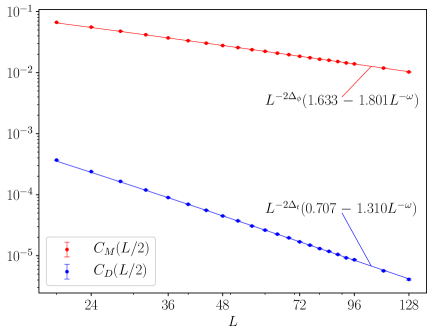
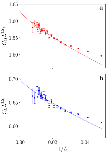
To test the scaling form ${L^{-(1+\eta_{d})}}={L^{-2\Delta_{t}}}$, we analyze the oscillating part $C_{D}(L/2)$ of the dimer-dimer correlation function. Since the connection between the primary order parameter and $\Delta_{\phi}$ is well known, we first used its scaling behavior to refine the value of $\Gamma_{c}$ reported in Ref. Wenzel et al. (2012), as detailed in Supplemental Material, Sec. SV sup , obtaining $\Gamma_{c}=1.57680\pm 0.00009$. We then calculated $C_{M}(L/2)$ and $C_{D}(L/2)$ at the midpoint; their scaling behaviors are shown in Fig. 4. The results match very well the scaling dimensions obtained in recent numerical conformal bootstrap calculations Chester et al. (2020): $\Delta_{\phi}\approx 0.519088$ and $\Delta_{t}\approx 1.23629$.

The simplest effective model with the same microscopic symmetries and exhibiting the same scaling behavior is a classical 3D 8-state clock model, where a charge-$l$ order parameter is defined by the vector $\vec{m}_{l}=(m_{x},m_{y})$, with $m_{x}=\sum_{i}\cos(l\theta_{i})$, $m_{y}=\sum_{i}\sin(l\theta)$, $\theta_{i}$ being the angle of spin $i$. Results for this model are presented in Supplemental Material, Sec SVI sup ). The excellent agreement with the expected exponents in both the FFTFIM and clock model confirms without doubt the emergent $U(1)$ symmetry and the primary and secondary nature of the order parameters in the FFTFIM.

Figure 4: Dimer-dimer (blue) and spin-spin (red) correlation functions at the quantum critical point, $\Gamma/J=1.5768$. The lines are fits of the $L\geq 44$ data to the expected scaling form $\propto L^{-2\Delta_{s,t}}(a+bL^{-\omega})$, with $\Delta_{\phi}=0.519088$, $\Delta_{t}=1.23629$ Chester et al. (2020), and the correction exponent $\omega=0.789$ Hasenbusch (2019) in the 3D $O(2)$ universality class. The reduced $\chi^{2}$ values are $\sim 0.8$ and $\sim 0.9$ for the spin and dimer correlations respectively.

Conclusion.—We have clarified the nature of the two order parameters, based on spins and dimers, in the square-lattice FFTFIM. The spin-based order parameter is primary, as it scales with the leading critical exponents and displays the full eight-fold degeneracy of the ordered phase, while the $Z_{4}$ dimer order parameter is secondary with faster decaying critical correlations. Our QMC results at $T=0$ and $T>0$ confirm the scaling exponents predicted from the respective low-energy field theories.

Mapping to dimer models is a powerful tool in the study of frustrated spin systems, and the problem of lattice coverings by hard-core dimers is an interesting topic in itself. The connection between the secondary dimer order parameter and the primary spin order parameter then provides a crucial link between the models that had not been previously drawn in this context. Beyond the particular FFTFIM considered here, the triangular and kagome lattice AF Ising models Nagai et al. (1993); Moessner and Sondhi (2001), the fully-frustrated honeycomb lattice Ising model Moessner and Sondhi (2001), and the fully frustrated 4-8 lattice Ising models Hearth et al. (2022) are all well studied systems where the secondary order parameter prescription could also be applied.

Our insights also explain the critical scaling of a so-called “parasitic” order parameter studied in the AF 3-state Potts model on the diamond lattice Hattori and Tsunetsugu (2016). While the observed scaling had previously eluded explanation, it is now clear that this secondary (parasitic) order parameter also has scaling dimension $\Delta_{t}$ in that system.

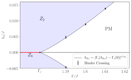
The relevance of the secondary order parameter operator ($\Delta_{t}<3$) in the FFTFIM implies that a perturbation favoring one of the dimer states, accomplished by appropriately modulating the Ising couplings, will induce a $Z_{2}$ symmetry breaking phase in the plane of $\Gamma$ and the dimer field (modulation) strength $h_{d}$. The phase boundary between the paramagnetic and ordered phases should have the asymptotic form $h_{d,c}\sim|\Gamma_{c}(h_{d,c})-\Gamma_{c}(0)|^{\nu/\nu_{d}}$, where $\nu$ is the 3D $O(2)$ correlation-length exponent and $\nu_{d}=(3-\Delta_{t})^{-1}$, which we confirm in Supplemental Material, Sec. SVII sup .

The FFTIFM, with $h_{d}=0$ and $h_{d}>0$, can be implemented on current D-Wave quantum annealing devices. The frustrated AFM triangular AF Ising model has already been studied King et al. (2018, 2021) and it would be interesting to consider also the square-lattice model and examine differences between the spin and dimer order parameters, in the light of our results.

Acknowledgments.—We would like to thank Fabien Alet, Ling Wang, and Sumner Hearth for useful discussions. This work was supported by the Simons Foundation under Grant No. 511064, by the National Natural Science Foundation of China under Grants No. 12122502 and No. 12175015, and by the Swiss National Science Foundation under Grant No. 182179. Most of the numerical calculations were carried out on the Shared Computing Cluster managed by Boston University’s Research Computing Services.

SI Phase Diagram

The finite temperature phase diagram for the FFTFIM is shown in Fig. S1. At temperatures above $T_{\rm c2}(\Gamma)$, or transverse field values above $\Gamma_{c}$, the system is in the paramagnetic (PM) phase, while for $\Gamma<\Gamma_{c}$ and $T_{\rm c1}(\Gamma)<T<T_{\rm c2}(\Gamma)$, it is in a critical KT phase. For $\Gamma<\Gamma_{c}$ and $T<T_{\rm c1}(\Gamma)$, the system is ordered, exhibiting $Z_{8}$ and $Z_{4}$ symmetry breaking in the primary and secondary order parameters, respectively. The phase diagram was constructed in the following way:

Figure S1: Phase diagram of the square-lattice FFTFIM in the plane of transverse field $\Gamma$ and temperature $T$. The QCP is shown as the black circle at $T=0$. The black dashed lines are the theoretical predictions for the phase boundaries made in Ref. Jiang and Emig (2005); Korshunov (2012), and the red and blue points are the transition temperatures identified using our QMC simulations. The theoretical phase boundaries have overall unknown factors that we have adjusted for best agreement at the maximums.

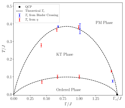
To locate the upper transition temperature $T_{\rm c2}$, we define Binder cumulants for both order parameters Binder (1981):

$$U_{d}=2-\frac{\langle|\Psi|^{4}\rangle}{\langle|\Psi|^{2}\rangle^{2}},\quad U_{m}=2-\frac{\langle|m|^{4}\rangle}{\langle|m|^{2}\rangle^{2}}.$$ (S1)

At the critical temperature, the Binder cumulant should be system-size dependent, and we indeed find that curves of $U$ versus $T$ for different $L$ values intersect each other close to a point $T_{\rm c2}$. We extract the temperatures at which the cumulants for pairs of system sizes $L$ and $2L$ intersect, and extrapolate these to the infinite-size $T_{\rm c2}$ using the expected finite-size scaling form (shift of a definition of the critical point with the system size) at a KT transition Hsieh et al. (2013):

$$\begin{split}T_{c2}(L)=T_{c2}(\infty)+\frac{a}{\log^{2}(aL)},\end{split}$$ (S2)

An example of this procedure is shown in Fig. S2 for $\Gamma/J=1.50$. The fits to the primary (red) and secondary (blue) binder crossing temperatures give infinite-size $T_{c2}$ valuess that agree well with each other to within error bars estimated using bootstrapping of the data.

Figure S2: Finite-size scaling of the Binder crossing temperature at $\Gamma/J=1.50$. The temperatures for the magnetization (red) and dimer (blue) order parameters were extracted for pairs of systems of size $(L,2L)$. The error bars on the extrapolated $T_{\rm c2}(\infty)$ values were estimated by a bootstrapping procedure.

At the lower phase boundary, between the KT phase and the ordered phase, we do not find any crossings of the Binder cumulants. Instead, we located $T_{\rm c1}$ from the expected power-law scaling of the magnetic and dimer order parameters, with exponents $\eta_{m}=1/16$ and $\eta_{d}=1/4$ at the lower boundary, supported also by the observed break-down of power-law scaling of the order parameters below $T_{\rm c1}$. Our analysis of the correlation functions is described in the main text and in more detail in Sec. SII.

The black point at $T=0$ in Fig. S1 is the quantum critical point (QCP), which was identified in Ref. Wenzel et al. (2012); we further refined its location in the present work as detailed below in Sec. SV. The black dashed lines show the theoretical scaling of $T_{\mathrm{c}i}$ versus $\Gamma$ predicted by Ref. Jiang and Emig (2005); Korshunov (2012), in which an overall factor has been adjusted to fit our data at the maximums. These phase boundaries are formally only valid for $\Gamma_{c}-\Gamma\ll\Gamma_{c}$ (near the QCP), but we include them here all the way to $\Gamma=0$ as a visual aid.

SII Height Model Mapping

Here, we make explicit the mapping between the spins, dimers, and height variables of the FFTFIM. Following the prescription in Ref. Jiang and Emig (2005); Korshunov (2012), we start by identifying the 2-to-1 mapping between the ground states of the classical fully frustrated Ising model and those of the purely kinetic dimer model on the square lattice Villain (1977b). These degenerate states are defined by the configurations where each plaquette contains a single frustrated bond. The dimer model on the square lattice has been studied extensively Fisher (1961); Rokhsar and Kivelson (1988); Alet et al. (2005) and its height representation is known Henley (1997). We repeat the mapping here for the specific sake of clarifying the relationship between the spin and dimer order parameters, which was not emphasized in previous treatments.

The mapping proceeds as follows: begin by dividing the dual lattice into two sublattices $A$ and $B$, where dimers connect dual lattice sites from sublattice $A$ to $B$. Assign an arbitrary height value to a site on the spin lattice and move clockwise around a dual lattice site. If the dual lattice site is on sublattice $A$ and a dimer is crossed, the height value at the following spin lattice site is increased by 3, otherwise it is reduced by 1; see Fig. S3. If the dual lattice site is on sublattice $B$, the same rules apply with signs reversed; -3 and +1, respectively.

Figure S3: Height model mapping rules for a plaquette at dual sublattice $A$. Height variables $h$ are labeled at the spin sites.

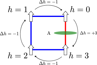
In the ordered phase, the dimers are ordered along columns or rows, corresponding to a height profile that is ”flat,” i.e., the height value at any given lattice site is bounded from above. In the critical and disordered phases, plaquettes with three frustrated bonds begin to populate the system. The height model is then ”rough”, with a logarithmically diverging height profile. This behavior can be described by an effective elastic free energy with a periodic ”locking” potential favoring flat height configurations Burton et al. (1997); Alet et al. (2005);

$$F(\{h(\vec{r})\})=\int d\vec{x}\,\left[\frac{K}{2}\big{|}\vec{\nabla}h(\vec{r})\big{|}+V\cos\left(2\pi h(\vec{r})\right)\right],$$ (S3)

where $h(\vec{r})$ is the coarse-grained height field (height variables averaged over a plaquette), $K$ is the temperature dependent stiffness constant, and $V>0$ is the strength of the locking potential.

As discussed in the main text, for $T<T_{c1}$ the locking potential is a relevant perturbation and the system orders José et al. (1977); Henley (1997). For $T_{c1}<T<T_{c2}$, ”screw dislocations” begin to emerge in pairs throughout the system. These defects are the aforementioned plaquettes containing not one but three frustrated bonds, which appear bound in neutral pairs. For $T>T_{c2}$, the interaction between the defects becomes sufficiently weak for the pairs to unbind, spreading throughout the system and disordering the critical phase Jiang and Emig (2005, 2006); Korshunov (2012).

In the critical (rough) phase, the locking potential is irrelevant, and the system is described by a free Gaussian theory. The long distance height difference correlations can be easily calculated Nienhuis et al. (1984); Henley (1997); José et al. (1977):

$$\begin{split}\frac{1}{2}\langle\big{|}h(\vec{r})-h(\vec{0})\big{|}^{2}\rangle\propto\frac{\ln(r)}{2\pi K}.\end{split}$$ (S4)

We relate this form to the spin-spin and dimer-dimers correlations by noting that the spins are periodic in the height variables, with a period of 8. This can be seen by turning the spins around a plaquette twice as depicted in Fig. S4.

Figure S4: Demonstration of the periodicity of the spin variables with the height variables. Upon traversing the plaquette, each spin (marked in yellow) is flipped sequentially (left to right, upper then lower row) and the height variables are computed according to the rules laid out in the text. The final spin configuration is identical to the initial one, but with each height increased by 8, implying that the spins must be periodic in the heights with period 8.

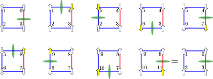
This periodicity implies that the spins can be written as a Fourier series:

$$\begin{split}\sigma^{z}(\vec{r})=\sum_{G}\tilde{\sigma}^{z}_{G}e^{iGh(\vec{r})}\end{split}$$ (S5)

where $G=\frac{2\pi}{8}n$ with $n=1,2,3,\dots$. The spin-spin correlations for a single Fourier mode is given by

$$\begin{split}\langle e^{iGh(\vec{r})}e^{-iGh(\vec{0})}\rangle=e^{-\frac{1}{2}G^{2}\langle|h(\vec{r})-h(\vec{0})|^{2}\rangle},\end{split}$$ (S6)

and clearly the smallest $G$ value in the expansion in Eq. (S5) will dominate. Thus, we can express the coarse-grained spin and dimers as

$$\begin{split}&\sigma^{z}(\vec{r})\propto e^{i\frac{2\pi}{8}h(\vec{r})}\\ &d(\vec{r})\propto\sigma^{z}(\vec{x})\sigma^{z}(\vec{r}+\hat{x})\approx\left(\sigma^{z}(\vec{r})\right)^{2}\propto e^{i\frac{4\pi}{8}h(\vec{r})}.\end{split}$$ (S7)

Plugging in the height difference correlations in the rough phase, Eq. (S4), we can extract the anomalous dimensions for the spins and dimers:

$$\begin{split}\langle\sigma^{z}(\vec{x})\sigma^{z}(\vec{0})\rangle&\propto e^{-\frac{1}{2}\left(\frac{2\pi}{8}\right)^{2}\langle|h(\vec{r})-h(\vec{0})|^{2}\rangle}\\ &\propto r^{-{\pi}/{32K}}\propto r^{-\eta_{m}}\\ \langle d(\vec{r})d(\vec{0})\rangle&\propto e^{-\frac{1}{2}\left(\frac{24pi}{8}\right)^{2}\langle|h(\vec{r})-h(\vec{0})|^{2}\rangle}\\ &\propto r^{-{\pi}/{8K}}\propto r^{-\eta_{d}}\end{split}$$ (S8)

This mapping implies that $\eta_{d}=4\eta_{m}$, which we have confirmed numerically in Fig. 3c in the main text.

The above derived relationship between $\eta$ and $K$ allows us to determine the values of anomalous dimension at the boundaries of the critical phase. Because the effective free energy in Eq. (S3) is exactly that of the 2D classical XY model with an eight-state clock anisotropy term, we can use the RG analysis preformed in Ref. José et al. (1977) to determine the critical values of the coupling $K$ separating the critical phase from the ordered and disordered phases.

The lower and upper critical temperatures correspond to $K_{c1}=\pi/2$ and $K_{c2}=\pi/16$, between which the system is critical (cf. with Ref. Nienhuis et al. (1984)). The values of $\eta_{m}$ at the phase boundaries are then

$$\eta_{m}(T_{c1})=1/16,~{}~{}~{}\eta_{m}(T_{c2})=1/4.$$ (S9)

SIII Reduced $\chi^{2}$ for Power Law Fit in Critical Phase

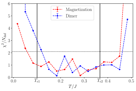
Below the lower critical temperature $T_{c1}$, the order parameters should no longer scale as power laws. Around this temperature, we therefore expect that the reduced $\chi^{2}$ from a power law fit used to extract $\eta_{m}$ and $\eta_{d}$ would begin to degrade. Figure S5 shows the reduced $\chi^{2}$ for these fits versus temperature compared to the reference value corresponding to the 95% confidence level (black dashed line). The results are indeed consistent with the power law form no longer being applicable below $T_{c1}$ and above $T_{c2}$. Larger system sizes would be required to observe the fits deteriorating more significantly close to the phase boundary. The results shown here were obtained by including the largest 8 system sizes in Figs. 3(a) and 3(b) in the fits.

Figure S5: Reduced $\chi^{2}$ values from power law fits used to extract $\eta_{m}$ (red) and $\eta_{d}$ (blue) in Fig. 3 of the main text. The black dashed line denotes the value corresponding to the 95% confidence level for the number of degrees of freedom of the fits. The reduced $\chi^{2}$ begins to exceed the 95% confidence level below $T_{c1}$ and above $T_{c2}$, indicating that the order parameters no longer scale as power laws.

SIV Correlation Function at Zero Temperature

At the quantum critical point, we measure the long distance correlation functions to extract the scaling exponents $\eta_{m}$ and $\eta_{d}$ at $T=0$. The spin-spin correlation function is defined as

$$\lim_{r\to\infty}C_{M}(\vec{r})=\lim_{r\to\infty}\langle\sigma^{z}_{m_{i}}(\vec{r})\sigma^{z}_{m_{i}}(0)\rangle\sim\frac{1}{r^{1+\eta_{m}}},$$ (S10)

where $\sigma^{z}_{m_{i}}(\vec{r})$ is the spin operator at a site $\vec{r}$ on sublattice $i$ and we expect $\eta_{m}=\eta_{\mathrm{3D}XY}$. In connection to the relevant field theory, $1+\eta_{\mathrm{3D}XY}=2\Delta_{\phi}$, where $\Delta_{\phi}\approx 0.519088$ Chester et al. (2020) is the scaling dimension of the order parameter of the 3D $O(2)$ model. This reflects the known irrelevance of $Z_{q}$ perturbations with $q\geq 4$ at this critical point.

The dimer-dimer correlation function is defined as

$$D_{x}(\vec{r})=\langle d_{x}(\vec{r})d_{x}(0)\rangle,$$ (S11)

where $d_{x}(\vec{r})$ is the $x$-oriented dimer operator at a site $\vec{r}$. However, in the ordered phase, the dimer correlations will oscillate between smaller and larger values and the order parameter of interest is the difference between these modulated correlations;

$$D^{*}_{x}(\vec{r})=D_{x}(\vec{r})-\frac{D_{x}(\vec{r}-\hat{y})+D_{x}(\vec{r}+\hat{y})}{2}.$$ (S12)

Averaging over both horizontal and vertical dimer orientations, the expected scaling is

$$\lim_{r\to\infty}C_{D}(\vec{r})=\lim_{r\to\infty}\frac{D^{*}_{x}(\vec{r})+D^{*}_{y}(\vec{r})}{2}\sim\frac{1}{r^{1+\eta_{d}}}$$ (S13)

We evaluate both of these correlation functions at the largest separation for a periodic, finite system of linear size $L$, $\vec{r}=(L/2,L/2)$. In Fig. 4 of the main text we show that the dimer correlations fall off with distance as a power law with exponent corresponding to the leading charge-2 operator of the 3D $O(2)$ model; $1+\eta_{d}=2\Delta_{t}$, with $\Delta_{t}\approx 1.23629$ Chester et al. (2020).

SV Determining $\mathbf{\Gamma_{c}}$

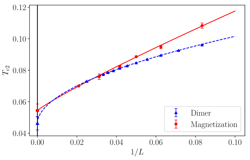
To determine $\Gamma_{c}$, we located the value of $\Gamma$ where the primary order parameter correlation functions scales as power law with the expected power $\Delta_{\phi}$. We measured the correlations function for $\Gamma$ values in a small range around the previously reported $\Gamma_{c}$ and compared the $\chi^{2}$ from power law fits to the data at these different values. To reduce the error bars on the measured data, we interpolated the correlation function data for a given system size using second-order polynomials for several data sets in the $\Gamma$ range $\left[1.576,1.578\right]$.

Figure S6: Reduced $\chi^{2}$ from power-law fits to the spin-spin correlation function data versus $\Gamma$. The $\chi^{2}$ minimum converges as the smallest $L$ value used in the fit is increased. Using the number of degrees of freedom for the $L_{\rm min}=44$ fit, we determine the $\Gamma$ values within the 95% confidence interval of the $\chi^{2}$ distribution, indicated here by the two vertical black lines. The error bars were computed by bootstrapping the raw binned data sets.

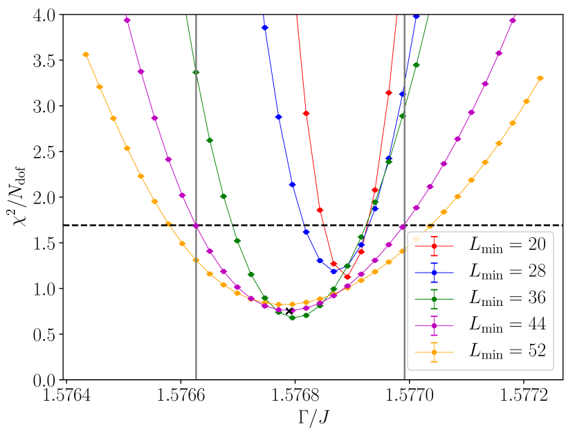
Reduced $\chi^{2}$ versus $\Gamma$ for the spin-spin correlation function is shown in Fig. S6, where we see convergence in the location of the $\chi^{2}$ minimum as the minimum system size used for the fit is increased. We judge that any remaining systematic errors from scaling corrections are negligible for $L_{\rm min}=44$, and the resulting critical point is then $\Gamma_{c}=1.57680\pm 0.00009$. To determine the error bar on $\Gamma_{c}$, we located $\Gamma$ values where the reduced $\chi^{2}$ is equal to the the 95% confidence level for the number of degrees of freedom used, denoted by the two vertical black lines.

SVI Secondary Order Parameter in 3D Classical Clock Models

The 3D classical $q$-state clock model is defined by the Hamiltonian

$$H_{q}=-\sum_{\langle i,j\rangle}\cos\left(\theta_{i}-\theta_{j}\right)-h_{q}\sum_{i}\cos\left(q\theta_{i}\right),$$ (S14)

with $\theta_{i}\in\left[0,2\pi\right)$ defining the orientation of a two-component spin on cubic lattice site $i$. At fixed $h_{q}$, below $T=T_{\rm c}$, the systems orders into a $Z_{q}$ symmetry breaking phase. The $Z_{q}$ perturbation for $q\geq 4$ is known to be irrelevant at the critical point, so that the 3D $O(2)$ universality class applies (though changing the symmetry broken in the ordered phase).

For $q=8$, the microscopic symmetries of the model exactly match those of the square-lattice FFTFIM, and we here study this clock model as a bench-mark case of primary and secondary order parameters. Just as in the FFTFIM, we can define charge-1 and charge-2 scalar order parameters for the clock models:

$$\begin{split}m_{x}=\sum_{i}\cos(l\theta_{i})&,~{}~{}m_{y}=\sum_{i}\sin(l\theta_{i}),\\ m_{l}^{2}=&\langle m_{x}^{2}\rangle+\langle m_{y}^{2}\rangle,\end{split}$$ (S15)

where $l$ labels the charge.

Figure S7: Scaling behaviors of $m_{l}^{2}$, with charge $l=1$ i (a) and $l=2$ in (b), at the estimated critical temperatures for the $q=4$ and $q=8$ clock models (using $1/T_{c}=0.45416467$ for $q=8$ Hasenbusch (2019) and $T_{c}=2.20467$ for $q=4$. The curves show the form Eq. (S16) with only the constants $a$ and $b$ adjusted for best fits and with results for the smaller system sizes exccluded systematically until a statistically good reduced $\chi^{2}$ value is obtained.

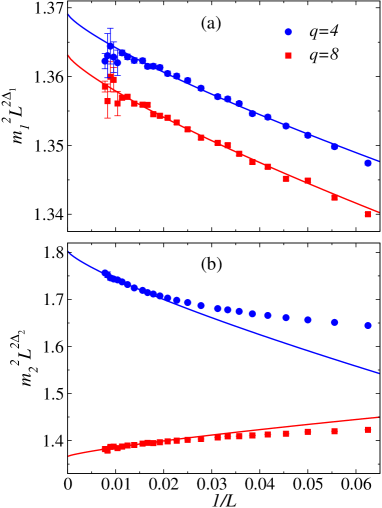
Although our primary interest here is in the $q=8$ case, we carried out simulations at the critical points of three different versions of the model, namely, the XY model (with no clock field, corresponding to $q\to\infty$), the 8-state hard clock model (with the spins restricted to the $q$ discrete states, corresponding to $h_{8}\to\infty$), and the 4-state soft clock model with anisotropic field $h_{4}=1$. We expect the same scaling dimensions in all cases on account of the irrelevance of the clock perturbations. The critical points of the first two models can be found in Ref. Hasenbusch (2019), while $T_{c}=2.20465(1)$ of the third model was reported in Shao et al. (2020). In an improved analysis, we found this value to be about two error bars too low and here report results obtained with $T=2.20467$.

Figure S8: Scaling behaviors of $C_{M}(L/2)$ and $C_{D}(L/2)$, plotted as in Fig. S7.

In Fig. S7 we fit our data for $q=4$ and $q=8$ to the expected scaling form with the leading finite-size correction included;

$$m_{l}^{2}L^{2\Delta_{l}}=a+bL^{-\omega}$$ (S16)

with $\Delta_{1}=\Delta_{\phi}=0.519088$, $\Delta_{2}=\Delta_{t}=1.23629$ Chester et al. (2020), and $\omega=0.789$ Hasenbusch (2019). Only the prefactors $a$ and $b$ were fitted. In the case of the XY model, the results fall so close to those for $q=8$ that we have not included them in the figure for clarity (we also note that the error bars are larger for the XY model after simulations of comparable length).

To compare the clock results more directly to the FFTFIM results shown in Fig. 4 of the main text, in Fig. S8 we show the FFTIFM data analyzed in the same way as the clock results in Fig. S7, with the expected leading power laws of $L$ divided out and fitting only to the expected correction given by Eq. (S16). Though the sign of the (non-universal) amplitude of the correction to the dimer correlations in Fig. S8(b) is different from that in the $q=8$ result in Fig. S7(b), the overall behavior of the corrections (the leading term fitted to and the higher-order corrections causing deviations from the fit) is similar. The primary order parameter of the FFTFIM in Fig. S8(a) seems to have more significant subleading corrections than the clock results in Fig. S7, but the large-$L$ asymptotic form is again similar and consistent with the leading correction.

Figure S9: $\Gamma$–$h_{d}$ phase boundary. The red line indicates the $Z_{8}$-breaking phase that exists only at $h_{d}=0$. The black dashed lines show the boundaries between the paramagnetic and $Z_{2}$-breaking phases and are of the form given in Eq. (S18), where a single prefactor was adjusted to fit the data.

SVII $\mathbf{Z_{2}}$ Phase

By alternating the Ising couplings betweek $J-h_{d}$ and $J+h_{d}$ ($J=1$) on either rows or columns in the FFTFIM, a single dimer state and its accompanying two spin states are energetically favored. Thus, this perturbation, arbitrarily weak, induces a $Z_{2}$ symmetry breaking phase in the plane of $\Gamma$ and the strength of the coupling modulation $h_{d}$.

We can derive the expected asymptotic form of the phase boundary by considering the diverging length scales corresponding to each perturbing field ($\Gamma$ and $h_{d}$). Upon tuning $\Gamma\to\Gamma_{c}$ and $h_{d}\to h_{d,c}$, their respective correlation lengths will diverge as

$$\xi_{\Gamma}\sim|\Gamma-\Gamma_{c}|^{-\nu},~{}~{}\xi_{h_{d}}\sim|h_{d}-h_{d,c}|^{-\nu_{d}},$$ (S17)

where $\nu$ again is the 3D $O(2)$ correlation length exponent, $\nu=(3-\Delta_{s})^{-1}$ in terms of the relevant charge-0 (singlet) scaling dimension $\Delta_{s}\approx 1.51136$ Chester et al. (2020), and $\nu_{d}=(3-\Delta_{t})^{-1}$ with $\Delta_{t}=1.23629$. Assuming that the $\Gamma$–$h_{d}$ phase boundary corresponds to a fixed ratio of these two length scales, we extract the form

$$h_{d,c}\sim|\Gamma_{c}(h_{d,c})-\Gamma_{c}(0)|^{\nu/\nu_{d}}.$$ (S18)

We have confirmed this form using numerics, as shown in Fig. S9, using the same type of QMC simulations and analysis as explained in previous sections.

References

- Villain (1977a) J. Villain, Journal of Physics C: Solid State Physics 10, 1717 (1977a).
- Villain, J. et al. (1980) Villain, J., Bidaux, R., Carton, J.-P., and Conte, R., J. Phys. France 41, 1263 (1980).
- Moessner (2001) R. Moessner, Canadian Journal of Physics 79, 1283 (2001).
- Henley (1989) C. L. Henley, Phys. Rev. Lett. 62, 2056 (1989).
- Coletta et al. (2014) T. Coletta, S. E. Korshunov, and F. Mila, Phys. Rev. B 90, 205109 (2014).
- Wenzel et al. (2012) S. Wenzel, T. Coletta, S. E. Korshunov, and F. Mila, Phys. Rev. Lett. 109, 187202 (2012).
- Dabholkar et al. (2022) B. Dabholkar, G. J. Sreejith, and F. Alet, Phys. Rev. B 106, 205121 (2022).
- Korshunov (2012) S. E. Korshunov, Phys. Rev. B 86, 014429 (2012).
- Blankschtein et al. (1984a) D. Blankschtein, M. Ma, and A. N. Berker, Phys. Rev. B 30, 1362 (1984a).
- (10) See Supplemental Material at [url to be inserted by publisher] for the phase diagram, Binder-crossing finite-size scaling, height model mapping, analysis of correlation functions, determination of , results for 3D classical clock model, and the phase boundary, which includes Refs. Binder (1981); Hsieh et al. (2013); Fisher (1961); Rokhsar and Kivelson (1988); Alet et al. (2005); Burton et al. (1997); Shao et al. (2020).
- Sandvik (2003) A. W. Sandvik, Phys. Rev. E 68, 056701 (2003).
- Wu et al. (1994) L. Wu, M. J. Young, Y. Shao, C. W. Garland, R. J. Birgeneau, and G. Heppke, Phys. Rev. Lett. 72, 376 (1994).
- Aharony et al. (1995) A. Aharony, R. J. Birgeneau, C. W. Garland, Y.-J. Kim, V. V. Lebedev, R. R. Netz, and M. J. Young, Phys. Rev. Lett. 74, 5064 (1995).
- Hasenbusch and Vicari (2011) M. Hasenbusch and E. Vicari, Phys. Rev. B 84, 125136 (2011).
- Netz and Aharony (1997) R. R. Netz and A. Aharony, Phys. Rev. E 55, 2267 (1997).
- Calabrese and Parruccini (2005) P. Calabrese and P. Parruccini, Phys. Rev. B 71, 064416 (2005).
- José et al. (1977) J. V. José, L. P. Kadanoff, S. Kirkpatrick, and D. R. Nelson, Phys. Rev. B 16, 1217 (1977).
- Blankschtein et al. (1984b) D. Blankschtein, M. Ma, A. N. Berker, G. S. Grest, and C. M. Soukoulis, Phys. Rev. B 29, 5250 (1984b).
- Blöte and Nightingale (1993) H. W. J. Blöte and M. P. Nightingale, Phys. Rev. B 47, 15046 (1993).
- Isakov and Moessner (2003) S. V. Isakov and R. Moessner, Phys. Rev. B 68, 104409 (2003).
- Moessner and Sondhi (2001) R. Moessner and S. L. Sondhi, Phys. Rev. B 63, 224401 (2001).
- Stephenson (2003) J. Stephenson, Journal of Mathematical Physics 11, 413 (2003), https://pubs.aip.org/aip/jmp/article-pdf/11/2/413/7519770/413_1_online.pdf .
- Jiang and Emig (2005) Y. Jiang and T. Emig, Phys. Rev. Lett. 94, 110604 (2005).
- Henley (1997) C. L. Henley, Journal of Statistical Physics 89, 483 (1997).
- Nienhuis et al. (1984) B. Nienhuis, H. J. Hilhorst, and H. W. J. Blote, Journal of Physics A: Mathematical and General 17, 3559 (1984).
- Campostrini et al. (2006) M. Campostrini, M. Hasenbusch, A. Pelissetto, and E. Vicari, Phys. Rev. B 74, 144506 (2006).
- Chester et al. (2020) S. M. Chester, W. Landry, J. Liu, D. Poland, D. Simmons-Duffin, N. Su, and A. Vichi, Journal of High Energy Physics 2020, 142 (2020).
- Hasenbusch (2019) M. Hasenbusch, Phys. Rev. B 100, 224517 (2019).
- Nagai et al. (1993) O. Nagai, S. Miyashita, and T. Horiguchi, Phys. Rev. B 47, 202 (1993).
- Hearth et al. (2022) S. N. Hearth, S. C. Morampudi, and C. R. Laumann, Phys. Rev. B 105, 195101 (2022).
- Hattori and Tsunetsugu (2016) K. Hattori and H. Tsunetsugu, Journal of the Physical Society of Japan 85, 094001 (2016), https://doi.org/10.7566/JPSJ.85.094001 .
- King et al. (2018) A. D. King et al., Nature 560, 456 (2018).
- King et al. (2021) A. D. King et al., Nature Communications 12, 1113 (2021).
- Binder (1981) K. Binder, Phys. Rev. Lett. 47, 693 (1981).
- Hsieh et al. (2013) Y.-D. Hsieh, Y.-J. Kao, and A. W. Sandvik, Journal of Statistical Mechanics: Theory and Experiment 2013, P09001 (2013).
- Fisher (1961) M. E. Fisher, Phys. Rev. 124, 1664 (1961).
- Rokhsar and Kivelson (1988) D. S. Rokhsar and S. A. Kivelson, Phys. Rev. Lett. 61, 2376 (1988).
- Alet et al. (2005) F. Alet, J. L. Jacobsen, G. Misguich, V. Pasquier, F. Mila, and M. Troyer, Phys. Rev. Lett. 94, 235702 (2005).
- Burton et al. (1997) J. K. Burton, Jr., and C. L. Henley, Journal of Physics A 30, 8385 (1997).
- Shao et al. (2020) H. Shao, W. Guo, and A. W. Sandvik, Phys. Rev. Lett. 124, 080602 (2020).
- Villain (1977b) J. Villain, Journal of Physics C: Solid State Physics 10, 1717 (1977b).
- Jiang and Emig (2006) Y. Jiang and T. Emig, Phys. Rev. B 73, 104452 (2006).
Supplementary Materials for “Primary and Secondary Order Parameters in the Fully Frustrated Transverse Field Ising Model on the Square Lattice”
Gabe Schumm, Hui Shao, Wenan Guo, Frédéric Mila, Anders W. Sandvik