Generalized Simplicial Attention Neural Networks

Abstract

The aim of this work is to introduce Generalized Simplicial Attention Neural Networks (GSANs), i.e., novel neural architectures designed to process data defined on simplicial complexes using masked self-attentional layers. Hinging on topological signal processing principles, we devise a series of self-attention schemes capable of processing data components defined at different simplicial orders, such as nodes, edges, triangles, and beyond. These schemes learn how to weight the neighborhoods of the given topological domain in a task-oriented fashion, leveraging the interplay among simplices of different orders through the Dirac operator and its Dirac decomposition. We also theoretically establish that GSANs are permutation equivariant and simplicial-aware. Finally, we illustrate how our approach compares favorably with other methods when applied to several (inductive and transductive) tasks such as trajectory prediction, missing data imputation, graph classification, and simplex prediction.

I Introduction

Over the past few years, the rapid and expansive evolution of deep learning techniques has significantly enhanced the state-of-the-art in numerous learning tasks. From Feed-Forward [2] to Transformer [3], via Convolutional [4] and Recurrent [5] Neural Networks, increasingly sophisticated architectures have driven substantial advancements from both theoretical and practical standpoints. In today’s world, data defined on irregular domains (e.g., graphs) are ubiquitous, with applications spanning social networks, recommender systems, cybersecurity, sensor networks, and natural language processing. Since their introduction [6, 7], Graph Neural Networks (GNNs) have demonstrated remarkable results in learning tasks involving data defined over a graph domain. Here, the versatility of neural networks is combined with prior knowledge about data relationships, expressed in terms of graph topology. The literature on GNNs is extensive, with various approaches explored, primarily grouped into spectral [8, 9] and non-spectral methods [10, 11, 12]. In a nutshell, the idea is to learn from data defined over graphs by computing a principled representation of node features through local aggregation with the information gathered from neighbors, defined by the underlying graph topology. This simple yet powerful concept has led to exceptional performance in many tasks such as node or graph classification [9],[13],[10] and link prediction [14], to name a few. At the same time, the introduction of attention mechanisms has significantly enhanced the performance of deep learning techniques. Initially introduced to handle sequence-based tasks [15],[16], these mechanisms allow for variable-sized inputs and focus on the most relevant parts of them. Attention-based models (including Transformers) have a wide range of applications, from learning sentence representations [17] to machine translation [15], from machine reading [18] to multi-label image classification [19], achieving state-of-the-art results in many of these tasks.

Pioneering works have generalized attention mechanisms to data defined over graphs [13, 20, 21]. However, despite their widespread use, graph-based representations can only account for pairwise interactions. As a result, graphs may not fully capture all the information present in complex interconnected systems, where interactions cannot be reduced to simple pairwise relationships. This is particularly evident in biological networks, where multi-way links among complex substances, such as genes, proteins, or metabolites exist [22]. Recent works on Topological Signal Processing (TSP) [23, 24, 25, 26, 27] have shown the advantages of learning from data defined on higher-order complexes, such as simplicial or cell complexes. These topological structures possess a rich algebraic description and can readily encode multi-way relationships hidden within the data. This has sparked interest in developing (deep) neural network architectures capable of handling data defined on such complexes, leading to the emergence of the field of Topological Deep Learning [28, 29]. In the sequel, we review the main topological neural network architectures, with emphasis to those built to process data on simplicial complexes (SCs).

Related Works. Recently, several neural architectures for simplicial data processing have been proposed. In [30], the authors introduced the concept of simplicial convolution, which was then exploited to build a principled simplicial neural network architecture that generalizes GNNs by leveraging on higher-order Laplacians. However, this approach does not enable separate processing for the lower and upper neighborhoods of a simplicial complex. Then, in [31], message passing neural networks (MPNNs) were adapted to simplicial complexes [32], and a Simplicial Weisfeiler-Lehman (SWL) coloring procedure was introduced to differentiate non-isomorphic SCs. The aggregation and updating functions in this model are capable of processing data exploiting lower and upper neighborhoods, and the interaction of simplices of different orders. The architecture in [31] can also be viewed as a generalization of the architectures in [33] and [34], with a specific aggregation function provided by simplicial filters [35]. In [36], recurrent MPNNs architectures were considered for flow interpolation and graph classification tasks. The works in [37, 38] introduced simplicial convolutional neural networks architectures that explicitly enable multi-hop processing based on upper and lower neighborhoods. These architectures also offer spectral interpretability through the definition of simplicial filters and simplicial Fourier transform [35], leveraging the interaction of simplices of different orders [38]. Then, the work in [39] introduced equivariant message passing simplicial networks; finally, in [40], the authors proposed a multi layer perceptron (MLP)-based simplicial architecture.

Self-attention schemes for simplicial neural networks were initially proposed in [1], which is the preliminary (preprint) version of this paper. Also, in a completely parallel and independent fashion, the paper in [41] proposed an attention mechanism for simplicial neural networks similar to the one in [1]. However, as we will elaborate later, in this paper we generalize the approach in [1], diverging also from the one in [41] in several key aspects. Our work, along with the one in [41], paved the way for the development of the topological attention framework in [42]. Finally, a simplicial-based attention mechanism for heterogeneous graphs was presented in [43].

Contribution. The primary objective of this paper is to propose Generalized Simplicial Attention Neural Networks (GSANs), a novel topological architecture that exploits masked self-attention mechanisms to process data defined on simplicial complexes. Extending our preliminary work in [1], and hinging on the Dirac operator and its Dirac Decomposition [44, 45], GSANs process simplicial data through (data-driven) anisotropic convolutional filtering operations that consider the various neighborhoods defined by the simplicial topology. Notably, GSANs enable joint processing of data defined on different simplex orders through a weight-sharing mechanism, induced by the Dirac operator, thus making it both theoretically justified and computationally efficient. A sparse projection operator is also specifically designed to process the harmonic component of the data, i.e. to properly leverage its topological invariants (holes). From a theoretical perspective, we prove that GSANs are permutation equivariant and simplicial-aware. Interestingly, GSANs largely extend the preliminary SAN approach from [1] in terms of architecture design, theoretical justifications and results, and different processing tasks they can be applied to. Finally, we illustrate how GSANs compares favorably with other available methods when applied to several learning tasks such as: (i) Trajectory prediction on ocean drifters tracks data [31]; (ii) Missing data imputation in citation complexes [30],[37]; (iii) Molecular graph classification [31]; (iv) Simplex prediction in citation complexes [38].

To summarize, the contribution of this paper is threefold:

1. We introduce GSANs, a novel topological architecture that hinges on Dirac operator using masked self-attention mechanisms to process data defined on simplicial complexes. GSANs enable joint processing of data defined on different simplex orders through a weight-sharing mechanism induced by the Dirac decomposition.

2. We derive a rigorous theoretical analysis illustrating the permutation equivariance and the simplicial awareness of the proposed GSAN architecture.

3. We provide a detailed implementation of GSAN for reproducibility, also illustrating their excellent performance on several available simplicial and graph benchmarks.

With respect to the aforementioned literature, the closest works are [38], [42] and [41], but there are significant differences with our approach. Specifically, the convolutional architecture that we propose as a building block for GSAN (cf. (III-A)) can be seen as a novel, principled, low-complexity, specific case of the general convolutional architecture of [38]. However, there are two main differences: i) The architecture in [38] does not leverage any attention mechanism; ii) Even when comparing just the two convolutional architectures, the work in [38] does not employ the Dirac operator nor the harmonic projection. As a result, there is no weight-sharing in their case, leading to a larger number of parameters that, as we will demonstrate later in the numerical experiments, does not necessarily lead to better learning performance. Regarding the work in [41], the authors propose a simplicial attention mechanism, which however deeply differs from our approach. Indeed, unlike the MPNN architecture in [41], we employ a convolutional architecture grounded in TSP theory. Our model handles the interplay between different simplex orders, enabling multi-hop processing over the complex’s neighborhoods and a tailored processing of the harmonic data component. Also, we develop distinct attention mechanisms for different adjacencies, as opposed to the single attention function in [41]. Finally, even if our method can be cast into the general topological attentional framework in [42] (just as any GNN can be see as a particular case of the message passing framework [32]), our principled derivation based on formal arguments from TSP leads to a unique architecture and a novel theoretical analysis that is not readily derivable from [42].

Notation. Scalar, vector and matrix variables are indicated by plain letters a, bold lowercase letters $\mathbf{a}$, and bold uppercase letters $\mathbf{A}$, respectively. $[\mathbf{A}]_{i,j}$ is the $(i,j)$-th element of $\mathbf{A}$, $[\mathbf{A}]_{i}$ is the $i$-th row of $\mathbf{A}$, $\mathbf{I}$ is the identity matrix, and $\lambda_{MAX}(\mathbf{A})$ denotes the largest eigenvalue of the matrix $\mathbf{A}$. $\textrm{im}(\cdot)$, $\textrm{ker}(\cdot)$, and $\text{supp}(\cdot)$ denote the image, the kernel, and the support of a matrix, respectively; $\oplus$ is the direct sum of vector spaces. Also, $\mathbf{a}\,||\,\mathbf{b}$ denotes the concatenation between two vectors $\mathbf{a}$ and $\mathbf{b}$, and $||_{k=1}^{K}\mathbf{a}_{k}$ represents the concatenation of $K$ vectors. Similarly, $||_{k=1}^{K}\mathbf{A}_{k}$ denotes the concatenation of $K$ matrices, which happens over the common dimension (if the matrices are square, we assume horizontal concatenation). Finally, $\{\mathbf{a}_{k}\}_{k=1}^{K}$ and $\{\mathbf{A}_{k}\}_{k=1}^{K}$ represents the collection of $K$ vectors and matrices, respectively. Other specific notation is defined along the paper if necessary.

II Background on Topological Signal Processing

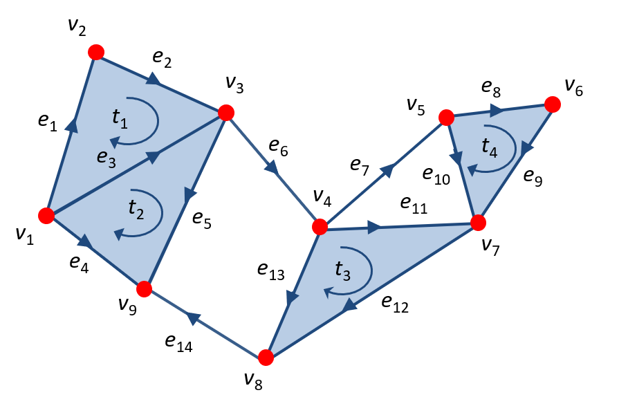
Figure 1: Representation of a order 2 simplicial complex $\mathcal{X}_{2}$ where $\mathcal{V}=\{v_{i}\}_{i=1}^{9}$, $\mathcal{E}=\{e_{i}\}_{i=1}^{14}$ and $\mathcal{T}=\{t_{i}\}_{i=1}^{4}$ denote, respectively, the set of vertices, edges and triangles.

In this section, we review some concepts from topological signal processing that will be useful to introduce the proposed GSANs architecture.

II-A Simplicial complex and signals

Given a finite set of vertices $\mathcal{V}$, a $k$-simplex $\mathcal{H}_{k,i}$ is a subset of $\mathcal{V}$ with cardinality $k+1$. A face of $\mathcal{H}_{k,i}$ is a subset with cardinality $k$ and thus a $k$-simplex has $k+1$ faces. A coface of $\mathcal{H}_{k,i}$ is a $(k+1)$-simplex that includes $\mathcal{H}_{k,i}$ [23][46]. If two simplices share a common face, then they are lower neighbours; if they share a common coface, they are upper neighbours [35]. A simplicial complex $\mathcal{X}_{K}$ of order $K$, is a collection of $k$-simplices $\mathcal{H}_{k,i}$, $k=0,\ldots,K$ such that, if a simplex $\mathcal{H}_{k,i}$ belongs to $\mathcal{X}_{K}$, then all its subsets $\mathcal{H}_{k-1,i}\subset\mathcal{H}_{k,i}$ also belong to $\mathcal{X}_{k}$ (inclusivity property). We denote the set of $k$-simplex in $\mathcal{X}_{K}$ as ${\cal D}_{k}:=\{\mathcal{H}_{k,i}:\mathcal{H}_{k,i}\in\mathcal{X}_{K}\}$, with cardinality $|{\cal D}_{k}|=N_{k}$.

In this paper, we are interested in processing signals defined over a simplicial complex. A $k$-simplicial signal is defined as a collection of mappings from the set of all $k$-simplices contained in the complex to real numbers:

$$\mathbf{x}_{k}=[x_{k}(\mathcal{H}_{k,1}),\dots,x_{k}(\mathcal{H}_{k,i}),\dots,x_{k}(\mathcal{H}_{k,N_{k}})]\in\mathbb{R}^{N_{k}},$$ (1)

where $x_{k}:{\cal D}_{k}\rightarrow\mathbb{R}$. The order of the signal is one less the cardinality of the elements of ${\cal D}_{k}$. In most of the cases the focus is on complexes of order up to two $\mathcal{X}_{2}$, thus having a set of vertices $\mathcal{V}$ with $|\mathcal{V}|=V$, a set of edges $\mathcal{E}$ with $|\mathcal{E}|=E$, and a set of triangles $\mathcal{T}$ with $|\mathcal{T}|=T$, which result in ${\cal D}_{0}={\cal V}$ (simplices of order 0), ${\cal D}_{1}={\cal E}$ (simplices of order 1), and ${\cal D}_{2}={\cal T}$ (simplices of order 2). In general, we define a simplicial complex (SC) signal as the concatenation of the signals of each order:

$$\mathbf{x}_{\mathcal{X}}=\big{[}\mathbf{x}_{0}\|\dots\|\mathbf{x}_{K}\big{]}\in\mathbb{R}^{\sum_{k=0}^{K}N_{k}}.$$ (2)

To give a simple example, in Fig. 1 we sketch a simplicial complex of order $2$. Therefore, the $k$-simplicial signals are defined as the following mappings:

$$x_{0}:{\cal V}\rightarrow\mathbb{R},\qquad x_{1}:{\cal E}\rightarrow\mathbb{R},\qquad x_{2}:{\cal T}\rightarrow\mathbb{R},$$ (3)

representing graph, edge and triangle signals, respectively. In this case, the corresponding SC signal is clearly given by:

$$\mathbf{x}_{\mathcal{X}}=\big{[}\mathbf{x}_{0}\|\mathbf{x}_{1}\|\mathbf{x}_{2}\big{]}\in\mathbb{R}^{N+E+T}.$$ (4)

II-B Algebraic representation

The structure of a simplicial complex ${\cal X}_{K}$ is fully described by the set of its incidence matrices $\mathbf{B}_{k}$, $k=1,\ldots,K$, given a reference orientation [47]. The entries of the incidence matrix $\mathbf{B}_{k}$ establish which $k$-simplices are incident to which $(k-1)$-simplices. We use the notation $\mathcal{H}_{k-1,i}\sim\mathcal{H}_{k,j}$ to indicate two simplices with the same orientation, and $\mathcal{H}_{k-1,i}\not\sim\mathcal{H}_{k,j}$ to indicate that they have opposite orientation. Mathematically, the entries of $\mathbf{B}_{k}$ are defined as follows:

$$\big{[}\mathbf{B}_{k}\big{]}_{i,j}=\left\{\begin{array}[]{rll}0,&\text{if}\;\mathcal{H}_{k-1,i}\not\subset\mathcal{H}_{k,j}\\ 1,&\text{if}\;\mathcal{H}_{k-1,i}\subset\mathcal{H}_{k,j}\;\text{and}\;\mathcal{H}_{k-1,i}\sim\mathcal{H}_{k,j}\\ -1,&\text{if}\;\mathcal{H}_{k-1,i}\subset\mathcal{H}_{k,j}\;\text{and}\;\mathcal{H}_{k-1,i}\not\sim\mathcal{H}_{k,j}\\ \end{array}\right..$$ (5)

As an example, considering a simplicial complex $\mathcal{X}_{2}$ of order two, we have two incidence matrices $\mathbf{B}_{1}\in\mathbb{R}^{V\times E}$ and $\mathbf{B}_{2}\in\mathbb{R}^{E\times T}$. From the incidence information, we can build the high order combinatorial Laplacian matrices [47], of order $k=0,\ldots,K$, as follows:

$$\mathbf{L}_{0}=\mathbf{B}_{1}\mathbf{B}_{1}^{T},$$ (6)

$$\mathbf{L}_{k}=\underbrace{\mathbf{B}_{k}^{T}\mathbf{B}_{k}}_{\mathbf{L}_{k}^{(d)}}+\underbrace{\mathbf{B}_{k+1}\mathbf{B}_{k+1}^{T}}_{\mathbf{L}_{k}^{(u)}},\;k=1,\ldots,K-1,$$ (7)

$$\mathbf{L}_{K}=\mathbf{B}_{K}^{T}\mathbf{B}_{K}.$$ (8)

All Laplacian matrices of intermediate order, i.e. $k=1,\ldots,K-1$, contain two terms: The first term $\mathbf{L}^{(d)}_{k}$, also known as lower Laplacian, encodes the lower adjacency of $k$-order simplices; the second term $\mathbf{L}_{k}^{(u)}$, also known as upper Laplacian, encodes the upper adjacency of $k$-order simplices. Thus, for example, two edges are lower adjacent if they share a common vertex, whereas they are upper adjacent if they are faces of a common triangle. Let us denote with $\mathcal{N}_{k,i}^{(d)}$ and $\mathcal{N}_{k,i}^{(u)}$ the lower and upper neighbors of the $i$-th simplex (comprising $i$ itself) of order $k$, respectively. Note that the vertices of a graph can only be upper adjacent, if they are incident to the same edge. This is why the Laplacian $\mathbf{L}_{0}$ contains only one term, and it corresponds to the usual graph Laplacian.

II-C Hodge decomposition

Hodge Laplacians admit a Hodge decomposition [46], leading to three orthogonal subspaces. In particular, the $k$-simplicial signal space can be decomposed as the direct sum of the following subspaces:

$$\mathbb{R}^{N_{k}}=\text{im}(\mathbf{B}_{k}^{T}\big{)}\oplus\text{im}\big{(}\mathbf{B}_{k+1}\big{)}\oplus\text{ker}\big{(}\mathbf{L}_{k}\big{)}.$$ (9)

Thus, any signal $\mathbf{x}_{k}$ of order $k$ can be decomposed as:

$$\mathbf{x}_{k}=\underbrace{\mathbf{B}_{k}^{T}\,\mathbf{x}_{k-1}}_{(a)}+\underbrace{\mathbf{B}_{k+1}\,\mathbf{x}_{k+1}}_{(b)}+\underbrace{\widetilde{\mathbf{x}}_{k}}_{(c)}.$$ (10)

Let us give an interpretation of the three orthogonal components in (10) considering edge signals $\mathbf{x}_{1}$ (i.e., $k=1$) [23],[37]:

(a)

Applying matrix $\mathbf{B}_{1}$ to an edge flow $\mathbf{x}_{1}$ means computing its net flow at each node, thus $\mathbf{B}_{1}$ is called a divergence operator. Its adjoint $\mathbf{B}_{1}^{T}$ differentiates a node signal $\mathbf{x}_{0}$ along the edges to induce an edge flow $\mathbf{B}_{1}^{T}\mathbf{x}_{0}$. We call $\mathbf{B}_{1}^{T}\mathbf{x}_{0}$ the irrotational component of $\mathbf{x}_{1}$ and $\text{im}(\mathbf{B}_{k}^{T})$ the gradient space.

(b)

Applying matrix $\mathbf{B}_{2}^{T}$ to an edge flow $\mathbf{x}_{1}$ means computing its circulation along each triangle, thus $\mathbf{B}_{2}^{T}$ is called a curl operator. Its adjoint $\mathbf{B}_{2}$ induces an edge flow $\mathbf{x}_{1}$ from a triangle signal $\mathbf{x}_{2}$. We call $\mathbf{B}_{2}\mathbf{x}_{2}$ the solenoidal component of $\mathbf{x}_{1}$ and $\text{im}(\mathbf{B}_{2})$ the curl space.

(c)

The remaining component $\widetilde{\mathbf{x}}_{1}$ is the harmonic component since it belongs to $\text{ker}(\mathbf{L}_{1})$ that is called the harmonic space. Any edge flow $\widetilde{\mathbf{x}}_{1}$ has zero divergence and curl.

II-D Dirac Decomposition

Although the Hodge Laplacians from (6)-(8) come with several favorable properties (e.g., Hodge decomposition and spectral representation), they can be only disjointly employed, i.e., the order $k$ Laplacian $\mathbf{L}_{k}$ can be used to process only $k-$simplicial signals $\mathbf{x}_{k}$, without any interplay with signals of different orders, if available. To overcome this limitation, we rely on the recently introduced Dirac operator [44, 45]. Given a simplicial complex $\mathcal{X}_{K}$ of order $K$ and a SC signal $\mathbf{x}_{\mathcal{X}}$, the Dirac operator is an indefinite operator that acts on $\mathbf{x}_{\mathcal{X}}$ and that can be written as a sparse block matrix $\mathbf{D}_{\mathcal{X}}\in\mathbb{R}^{\sum_{k=0}^{K}N_{k}\times\sum_{k=0}^{K}N_{k}}$ whose blocks are either zeros or the boundary operators $\{\mathbf{B}_{k}\}_{k=1}^{K}$, such that its square gives a block diagonal concatenation of the Laplacians $\{\mathbf{L}_{k}\}_{k=0}^{K}$:

$$\mathbf{D}_{\mathcal{X}}^{2}=\begin{bmatrix}\mathbf{L}_{0}&\mathbf{0}&\dots&\mathbf{0}\\ \mathbf{0}&\mathbf{L}_{1}&\dots&\mathbf{0}\\ \vdots&\vdots&\ddots&\vdots\\ \mathbf{0}&\mathbf{0}&\dots&\mathbf{L}_{K}\end{bmatrix}.$$ (11)

For instance, for a simplicial complex $\mathcal{X}_{2}$ of order two, the Dirac operator reads as:

$$\mathbf{D}_{\mathcal{X}}=\begin{bmatrix}\mathbf{0}&\mathbf{B}_{1}&\mathbf{0}\\ \mathbf{B}_{1}^{T}&\mathbf{0}&\mathbf{B}_{2}\\ \mathbf{0}&\mathbf{B}_{2}^{T}&\mathbf{0}\end{bmatrix}.$$ (12)

Due to its structure, it can be easily shown that a Dirac decomposition similiar to the Hodge decomposition in (10) holds [44]. In particular, for a simplicial complex $\mathcal{X}_{2}$ of order two, the Dirac decomposition is given by:

$$\mathbb{R}^{N+E+T}=\text{im}(\mathbf{D}_{\mathcal{X}}^{(d)}\big{)}\oplus\text{im}(\mathbf{D}_{\mathcal{X}}^{(u)}\big{)}\oplus\text{ker}\big{(}\mathbf{D}_{\mathcal{X}}\big{)},$$ (13)

where:

$$\mathbf{D}_{\mathcal{X}}^{(d)}=\begin{bmatrix}\mathbf{0}&\mathbf{B}_{1}&\mathbf{0}\\ \mathbf{B}_{1}^{T}&\mathbf{0}&\mathbf{0}\\ \mathbf{0}&\mathbf{0}&\mathbf{0}\end{bmatrix},\;\;\mathbf{D}_{\mathcal{X}}^{(u)}=\begin{bmatrix}\mathbf{0}&\mathbf{0}&\mathbf{0}\\ \mathbf{0}&\mathbf{0}&\mathbf{B}_{2}\\ \mathbf{0}&\mathbf{B}_{2}^{T}&\mathbf{0}\end{bmatrix}.$$ (14)

Therefore, also in this case we can give an interpretation of the spaces in (13) [45]; in particular, $\text{im}(\mathbf{D}_{\mathcal{X}}^{(d)}\big{)}$ is the joint gradient space, whereas $\text{im}(\mathbf{D}_{\mathcal{X}}^{(u)}\big{)}$ is the joint curl space.

II-E Simplicial complex filters

Generalizing the approach of [35, 45], we leverage the Dirac operator and the Dirac decomposition to introduce an extended definition of simplicial complex filters that reads as:

$$\mathbf{H}_{\mathcal{X}}=\underbrace{\sum_{j=1}^{J}w^{(d)}_{j}\big{(}\mathbf{D}_{\mathcal{X}}^{(d)}\big{)}^{j}}_{\mathbf{H}_{\mathcal{X}}^{(d)}}+\underbrace{\sum_{j=1}^{J}w^{(u)}_{j}\big{(}\mathbf{D}_{\mathcal{X}}^{(u)}\big{)}^{j}}_{\mathbf{H}_{\mathcal{X}}^{(u)}}+\underbrace{w^{(h)}\widetilde{\mathbf{Q}}}_{\mathbf{H}_{\mathcal{X}}^{(h)}},$$ (15)

where $\mathbf{w}^{(d)}=\Big{[}w^{(d)}_{1},...,w^{(d)}_{J}\Big{]}\in\mathbb{R}^{J}$, $\mathbf{w}^{(u)}=\Big{[}w^{(u)}_{1},...,w^{(u)}_{J}\Big{]}\in\mathbb{R}^{J}$ and $w^{(h)}\in\mathbb{R}$ are the filter weights, and $J\in\mathbb{N}$ is the filters order; the matrix $\widetilde{\mathbf{Q}}$ represents a sparse operator that approximates the orthogonal projector onto the harmonic space $\text{ker}\big{(}\mathbf{D}_{\mathcal{X}}\big{)}$, thus the summations in (15) start from 1 and not from 0, differently from [35, 45], to avoid that the harmonic component passes through the solenoidal and irrotational filters. Since from (13) it holds that $\text{ker}(\mathbf{D}_{\mathcal{X}})=\bigoplus_{k=0}^{K}\text{ker}(\mathbf{L}_{k})$, we can define $\widetilde{\mathbf{Q}}$ as a block diagonal matrix with the following structure:

$$\widetilde{\mathbf{Q}}=\begin{bmatrix}\widehat{\mathbf{Q}}_{0}&\mathbf{0}&\dots&\mathbf{0}\\ \mathbf{0}&\widehat{\mathbf{Q}}_{1}&\dots&\mathbf{0}\\ \vdots&\vdots&\ddots&\vdots\\ \mathbf{0}&\mathbf{0}&\dots&\widehat{\mathbf{Q}}_{K}\end{bmatrix},$$ (16)

with $\widehat{\mathbf{Q}}_{k}\in\mathbb{R}^{N_{k}\times N_{k}}$ being a sparse operator that approximates the orthogonal projector onto the harmonic space $\text{ker}\big{(}\mathbf{L}_{k}\big{)}$. In particular, from (9), harmonic signals can be represented as a linear combination of a basis of eigenvectors spanning the kernel of $\mathbf{L}_{k}$. However, since there is no unique way to identify a basis for such a subspace, the approximation can be driven by ad-hoc criteria to choose a specific basis, as in [25], [26]. Once defined a proper basis $\widetilde{\mathbf{U}}_{k}$, composed by eigenvectors of $\mathbf{L}_{k}$ corresponding to the zero eigenvalue of multiplicity $N_{h}\in\mathbb{N}$, the orthogonal projection operator onto $\text{ker}\big{(}\mathbf{L}_{k}\big{)}$ is given by $\mathbf{Q}_{k}=\widetilde{\mathbf{U}}_{k}\widetilde{\mathbf{U}}_{k}^{T}$. In general, the orthogonal projector $\mathbf{Q}_{k}$ is a dense matrix, but in practical applications sparse operators are clearly more appealing from the computational point of view. Thus, in (15)-(16), we build a sparse approximation of $\mathbf{Q}_{k}$ that enjoys distributed implementation and reads as [48]:

$$\widehat{\mathbf{Q}}_{k}=\big{(}\mathbf{I}-\epsilon\,\mathbf{L}_{k}\big{)}^{J},$$ (17)

where $0<\epsilon<\displaystyle\frac{2}{\lambda_{MAX}(\mathbf{L}_{k})}$. It can be shown that the operator $\widehat{\mathbf{Q}}_{k}$ in (17) enjoys the following property [48]:

$$\lim_{J\rightarrow\infty}\;\widehat{\mathbf{Q}}_{k}=\mathbf{Q}_{k}.$$ (18)

Please notice that the filter in (17) is given by the subsequent application of $J$ sparse matrices (depending on the $k$-th order Laplacian $\mathbf{L}_{k}$), which all enjoy nice locality properties that enable distributed implementation.

From (15), considering an order 2 SC $\mathcal{X}_{2}$, the simplicial complex filtering operation is given by $\mathbf{y}_{\mathcal{X}}=\mathbf{H}_{\mathcal{X}}\mathbf{x}_{\mathcal{X}},$ where $\mathbf{x}_{\mathcal{X}}=\big{[}\mathbf{x}_{0}\|\mathbf{x}_{1}\|\mathbf{x}_{2}\big{]}$ is the input signal and $\mathbf{y}_{\mathcal{X}}=\big{[}\mathbf{y}_{0}\|\mathbf{y}_{1}\|\mathbf{y}_{2}\big{]}$ is the output signal, with resulting input/output (I/O) relations that read as (obtained by simple direct computation) [35, 1]:

$$\mathbf{y}_{0}=\overset{\lfloor J/2\rfloor}{\underset{p=1}{\sum}}w_{2p}^{(d)}\big{(}\mathbf{L}_{0}\big{)}^{p}\mathbf{x}_{0}+\overset{\lceil J/2\rceil-1}{\underset{p=0}{\sum}}w_{2p+1}^{(d)}\big{(}\mathbf{L}_{0}\big{)}^{p}\mathbf{B}_{1}\mathbf{x}_{1}\vspace{.1cm}$$

$$\hskip 14.22636pt+w^{(h)}\widehat{\mathbf{Q}}_{0}\mathbf{x}_{0}$$

$$\mathbf{y}_{1}=\overset{\lfloor J/2\rfloor}{\underset{p=1}{\sum}}w_{2p}^{(d)}\big{(}\mathbf{L}^{(d)}_{1}\big{)}^{p}\mathbf{x}_{1}+\overset{\lceil J/2\rceil-1}{\underset{p=0}{\sum}}w_{2p+1}^{(d)}\big{(}\mathbf{L}_{1}^{(d)}\big{)}^{p}\mathbf{B}_{1}^{T}\mathbf{x}_{0}\vspace{.1cm}$$

$$\hskip 14.22636pt+\overset{\lfloor J/2\rfloor}{\underset{p=1}{\sum}}w_{2p}^{(u)}\big{(}\mathbf{L}^{(u)}_{1}\big{)}^{p}\mathbf{x}_{1}+\overset{\lceil J/2\rceil-1}{\underset{p=0}{\sum}}w^{(u)}_{2p+1}\big{(}\mathbf{L}_{1}^{(u)}\big{)}^{p}\mathbf{B}_{2}\mathbf{x}_{2}\vspace{.1cm}$$

$$\hskip 14.22636pt+w^{(h)}\widehat{\mathbf{Q}}_{1}\mathbf{x}_{1}$$

$$\mathbf{y}_{2}=\overset{\lfloor J/2\rfloor}{\underset{p=1}{\sum}}w_{2p}^{(u)}\big{(}\mathbf{L}_{2}\big{)}^{p}\mathbf{x}_{2}+\overset{\lceil J/2\rceil-1}{\underset{p=0}{\sum}}w_{2p+1}^{(u)}\big{(}\mathbf{L}_{2}\big{)}^{p}\mathbf{B}_{2}^{T}\mathbf{x}_{1}\vspace{.1cm}$$

$$\hskip 14.22636pt+w^{(h)}\widehat{\mathbf{Q}}_{2}\mathbf{x}_{2}.$$ (19)

The I/O relations in (II-E) correspond to applying certain specific filters on each order of the input simplicial signal. In particular, from (II-E), the filtered signal of the $k-$th order is the sum of a simplicial filter that processes the input signal of the same order $k$, a simplicial filter that processes the gradient of the $k+1$ simplicial signal (if available), and a simplicial filter that processes the curl of the $k-1$ simplicial signal (if available). Moreover, certain filter weights are shared: the coefficients of the filters in charge of processing same order simplicial signals and corresponding to the same Laplacian type (upper or lower) are all shared (e.g., $w_{2p}^{(d)}$ and $w_{2p}^{(u)}$ are the same per each order), and so are the coefficients of the filters in charge of processing other orders simplicial signals and corresponding to the same Laplacian type (the $w_{2p+1}^{(d)}$ and $w_{2p+1}^{(u)}$ are the same per each order). Notably, this represents a principled way of deriving a weight-sharing mechanism for the processing of simplicial-structured data, which is a well recognized practice in the design of deep learning models that gives clear computational advantages and, in this case, also spectral interpretation [45].

In the sequel, for clarity of exposition but without loss of generality, we will focus on order 2 simplicial complexes $\mathcal{X}_{2}$, even if our methodology can be applied to simplicial complexes of arbitrary order.

III Generalized Simplicial Attention
Neural Networks

In this section, we proceed by first introducing a generalized simplicial complex convolutional network (GSCCN) design, and then we equip it with self-attentional mechanisms to devise the proposed GSAN architecture. Finally, we will discuss its computational complexity, its theoretical properties, and the relations with other simplicial neural architectures.

III-A Generalized simplicial complex convolutional networks

We now design a GSCCN architecture, whose layers are composed of two main stages: i) bank of simplicial complex filtering as in (II-E), and ii) point-wise non-linearity. Let us assume that $F_{l}$ simplicial complex signals $\mathbf{Z}_{\mathcal{X},l}\in\mathbb{R}^{(N+E+T)\times F_{l}}$ are given as input to the $l$-th layer of the GSCCN, with $\mathbf{Z}_{0,l}=\{\mathbf{z}_{0,l,f}\}_{f=1}^{F_{l}}\in\mathbb{R}^{N\times F_{l}}$, $\mathbf{Z}_{1,l}=\{\mathbf{z}_{1,l,f}\}_{f=1}^{F_{l}}\in\mathbb{R}^{E\times F_{l}}$, and $\mathbf{Z}_{2,l}=\{\mathbf{z}_{2,l,f}\}_{f=1}^{F_{l}}\in\mathbb{R}^{T\times F_{l}}$ denoting the signals of each order. First, each of the input signals is passed through a bank of $F_{l+1}$ filters as in (II-E). Then, the intermediate outputs $\{\tilde{\mathbf{z}}_{k,l,f}\}_{f}$ are summed to avoid exponential filter growth and, finally, a pointwise non-linearity $\sigma_{l}(\cdot)$ is applied. Mathematically, the output signals $\mathbf{Z}_{\mathcal{X},l+1}$ of the $l-th$ layer read as:

$$\mathbf{Z}_{0,l+1}=\sigma_{l}\Bigg{(}\overset{\lfloor J/2\rfloor}{\underset{p=1}{\sum}}(\mathbf{L}_{0})^{p}\mathbf{Z}_{0,l}\mathbf{W}^{(d)}_{l,2p}$$

$$\hskip 19.91684pt\!+\!\!\!\!\!\overset{\lceil J/2\rceil-1}{\underset{p=0}{\sum}}\!\!(\mathbf{L}_{0})^{p}\mathbf{B}_{1}\mathbf{Z}_{1,l}\mathbf{W}^{(d)}_{l,2p+1}+\widehat{\mathbf{Q}}_{0}\mathbf{Z}_{0}\mathbf{W}^{(h)}_{l}\Bigg{)}$$

$$\mathbf{Z}_{1,l+1}=\sigma_{l}\Bigg{(}\overset{\lfloor J/2\rfloor}{\underset{p=1}{\sum}}(\mathbf{L}^{(d)}_{1})^{p}\mathbf{Z}_{1,l}\mathbf{W}^{(d)}_{l,2p}$$

$$\hskip 19.91684pt\!+\!\!\!\!\!\overset{\lceil J/2\rceil-1}{\underset{p=0}{\sum}}\!\!\!(\mathbf{L}^{(d)}_{1})^{p}\mathbf{B}_{1}^{T}\mathbf{Z}_{0,l}\mathbf{W}^{(d)}_{l,2p+1}+\sum_{p=1}^{\lfloor J/2\rfloor}(\mathbf{L}^{(u)}_{1})^{p}\mathbf{Z}_{1,l}\mathbf{W}^{(u)}_{l,2p}$$

$$\hskip 19.91684pt\!+\!\!\!\!\!\overset{\lceil J/2\rceil-1}{\underset{p=0}{\sum}}\!\!\!\!(\mathbf{L}^{(u)}_{1})^{p}\mathbf{B}_{2}\mathbf{Z}_{2,l}\mathbf{W}^{(u)}_{l,2p+1}+\widehat{\mathbf{Q}}_{1}\mathbf{Z}_{1}\mathbf{W}^{(h)}_{l}\Bigg{)}$$

$$\mathbf{Z}_{2,l+1}=\sigma_{l}\Bigg{(}\overset{\lfloor J/2\rfloor}{\underset{p=1}{\sum}}(\mathbf{L}_{2})^{p}\mathbf{Z}_{2,l}\mathbf{W}^{(u)}_{l,2p}$$

$$\hskip 14.22636pt+\overset{\lceil J/2\rceil-1}{\underset{p=0}{\sum}}(\mathbf{L}_{2})^{p}\mathbf{B}_{2}^{T}\mathbf{Z}_{1,l}\mathbf{W}^{(u)}_{l,2p+1}+\widehat{\mathbf{Q}}_{2}\mathbf{Z}_{2}\mathbf{W}^{(h)}_{l}\Bigg{)}.$$ (20)

The filters weights $\big{\{}\mathbf{W}^{(d)}_{l,p}\big{\}}_{p=1}^{J}$, $\big{\{}\mathbf{W}^{(u)}_{l,p}\big{\}}_{p=1}^{J}$ and $\mathbf{W}^{(h)}_{l}$ are learnable parameters (each matrix has dimesion $F_{l}\times F_{l+1}$), and are shared across modules processing different orders following the scheme in (II-E); the order $J$ of the filters, the number $F_{l+1}$ of output signals, and the non-linearity $\sigma_{l}(\cdot)$ are hyperparameters to be chosen (possibly) at each layer. Therefore, a GSCCN of depth $L$ with input data $\mathbf{X}_{\mathcal{X}}\in\mathbb{R}^{(N+E+T)\times F_{0}}$ is built as the stack of $L$ layers defined as in (III-A), where $\mathbf{Z}_{\mathcal{X},0}=\mathbf{X}_{\mathcal{X}}$. Based on the learning task at hand, an additional read-out layer can be inserted after the last GSCCN layer. In the sequel, building on the GSCCN layer in (III-A), we introduce the proposed GSAN architecture.

Figure 2: Architecture of the GSAN layer for a simplicial complex $\mathcal{X}_{2}$ of order two.

III-B Simplicial complex attention layer

We now proceed by equipping the GSCCN layer in (III-A) with a self-attentian mechanism, which generalizes the approaches in [13],[15], and our preliminary preprint in [1]. The core idea is to learn the coefficients of the higher-order Laplacian matrices - thus the weights of the diffusion over the complex - via topology-aware masked self-attention, in order to optimally combine data over the neighborhoods defined by the underlying topology in a totally data-driven fashion. From a signal processing perspective, this approach can be seen as a data-driven anisotropic filtering operation, i.e. it takes into account the different characteristics of the data being processed and, based on them, it applies a different strenght[49]. To this aim, let us introduce the attentional Laplacians associated to the $l$-th layer as

$$\begin{split}&\Big{[}\mathbf{L}^{(u,c_{k}^{(u)})}_{k,l}\Big{]}_{i,j}=\phi_{k,l,i,j}^{(u,c_{k}^{(u)})},\;\;k=0,1,\\ &\Big{[}\mathbf{L}^{(d,c_{k}^{(d)})}_{k,l}\Big{]}_{i,j}=\phi_{k,l,i,j}^{(d,c_{k}^{(d)})},\;\;\,k=1,2,\end{split}$$ (21)

where $c_{k}^{(u)}=1,2$ and $c_{k}^{(d)}=1,2$ are indexes associated with Laplacians (either upper $u$ or lower $d$) that appear twice in each filtering operation at order $k$. This allows us to process different signals in (III-A) using the same topological structure, but different diffusion weights. The attentional Laplacians in (21) encode topological information about the simplicial complex, i.e., their entries are masked to respect the connectivity of higher-order Laplacians. To incorporate the topological information, the masked attention coefficients in (21) are expressed as:

$$\phi_{k,l,i,j}^{(u,c_{k}^{(u)})}=\beta_{k,i,j}^{(u)}\cdot\alpha_{k,l,i,j}^{(u,c_{k}^{(u)})},\qquad\forall i,j,\;c_{k}^{(u)}=1,2$$ (22)

$$\phi_{k,l,i,j}^{(d,c_{k}^{(d)})}=\beta_{k,i,j}^{(d)}\cdot\alpha_{k,l,i,j}^{(d,c_{k}^{(d)})},\qquad\forall i,j,\;c_{k}^{(d)}=1,2$$ (23)

with $\beta_{k,i,j}^{(u)}=1$ if $j\in\mathcal{N}_{k,i}^{(u)}$ and 0 otherwise; similarly, $\beta_{k,i,j}^{(d)}=1$ if $j\in\mathcal{N}_{k,i}^{(d)}$ and 0 otherwise.

In the sequel, we will show how to learn the masked attention coefficients in (22) and (23). For the sake of exposition, we will focus on the edge level (1-simplices), but the same procedure applies to all the involved orders. The input to layer $l$ is $\mathbf{Z}_{\mathcal{X},l}=\{\mathbf{Z}_{k,l}\}_{k=0}^{2}\in\mathbb{R}^{(N+E+T)\times F_{l}}$, which collect the signals of each order. From (III-A), focusing on the edge level $k=1$, the first step is to apply a collection of shared learnable linear transformations parametrized by the filter weights $\big{\{}\mathbf{W}^{(d)}_{l,p}\big{\}}_{p=1}^{J}$ and $\big{\{}\mathbf{W}^{(u)}_{l,p}\big{\}}_{p=1}^{J}$ over all the involved signals. Then, let us introduce the following quantities:

$$\mathbf{h}_{1,l,2p,i}^{(u,1)}=[\mathbf{Z}_{1,l}\big{]}_{i}\mathbf{W}^{(u)}_{l,2p},\quad p=1,\ldots,\lfloor J/2\rfloor,$$

$$\mathbf{h}_{1,l,2p+1,i}^{(u,2)}=[\mathbf{B}_{2}\mathbf{Z}_{2,l}\big{]}_{i}\mathbf{W}^{(u)}_{l,2p+1},\quad p=0,\ldots,\lceil J/2\rceil-1,$$

$$\mathbf{h}_{1,l,2p,i}^{(d,1)}=[\mathbf{Z}_{1,l}\big{]}_{i}\mathbf{W}^{(d)}_{l,2p},\quad p=1,\ldots,\lfloor J/2\rfloor,$$

$$\mathbf{h}_{1,l,2p+1,i}^{(d,2)}=[\mathbf{B}_{1}^{T}\mathbf{Z}_{0,l}\big{]}_{i}\mathbf{W}^{(d)}_{l,2p+1},\quad p=0,\ldots,\lceil J/2\rceil-1,$$

which represent linear transformations of the input features, and are collected into the vectors:

$$\mathbf{h}_{1,l,i}^{(u,1)}=\overset{\lfloor J/2\rfloor}{\underset{p=1}{||}}\mathbf{h}_{1,l,2p,i}^{(u,1)}\in\mathbb{R}^{F_{l+1}\lfloor J/2\rfloor},$$

$$\mathbf{h}_{1,l,i}^{(u,2)}=\overset{\lceil J/2\rceil-1}{\underset{p=0}{||}}\mathbf{h}_{1,l,2p+1,i}^{(u,2)}\in\mathbb{R}^{F_{l+1}\lceil J/2\rceil},$$

$$\mathbf{h}_{1,l,i}^{(d,1)}=\overset{\lfloor J/2\rfloor}{\underset{p=1}{||}}\mathbf{h}_{1,l,2p,i}^{(d,1)}\in\mathbb{R}^{F_{l+1}\lfloor J/2\rfloor},$$

$$\mathbf{h}_{1,l,i}^{(d,2)}=\overset{\lceil J/2\rceil-1}{\underset{p=0}{||}}\mathbf{h}_{1,l,2p+1,i}^{(d,2)}\in\mathbb{R}^{F_{l+1}\lceil J/2\rceil}.$$ (24)

Let us now introduce the following attention mechanisms:

$$a^{(u,c_{1}^{(u)})}_{1,l}:\mathbb{R}^{F_{l+1}\lfloor J/2\rfloor}\times\mathbb{R}^{F_{l+1}\lfloor J/2\rfloor}\rightarrow\mathbb{R}$$ (25)

$$a^{(d,c_{1}^{(d)})}_{1,l}:\mathbb{R}^{F_{l+1}\lceil J/2\rceil}\times\mathbb{R}^{F_{l+1}\lceil J/2\rceil}\rightarrow\mathbb{R}$$ (26)

for $c_{1}^{(u)}=1,2$ and $c_{1}^{(d)}=1,2$. Practical examples of these mappings are given in the sequel. The attention coefficients are then computed as a function of the vectors in (24) as:

$$\gamma_{1,l,i,j}^{(u,c_{1}^{(u)})}=a^{(u,c_{1}^{(u)})}_{1,l}\left(\mathbf{h}_{1,l,i}^{(u,c_{1}^{(u)})},\mathbf{h}_{1,l,j}^{(u,c_{1}^{(u)})}\right)$$

$$\gamma_{1,l,i,j}^{(d,c_{1}^{(d)})}=a^{(u,c_{1}^{(d)})}_{1,l}\left(\mathbf{h}_{1,l,i}^{(d,c_{1}^{(d)})},\mathbf{h}_{1,l,j}^{(d,c_{1}^{(d)})}\right)$$ (27)

for $c_{1}^{(u)}=1,2$ and $c_{1}^{(d)}=1,2$. Finally, the normalized attention coefficients in (22) and (23) are obtained normalizing the attention coefficients in (27) (to make them easily comparable across different edges):

$$\alpha_{1,l,i,j}^{(u,c_{1}^{(u)})}={\rm softmax}_{j}(\gamma_{1,l,i,j}^{(u,c_{1}^{(u)})})=\frac{{\rm exp}(\gamma_{1,l,i,j}^{(u,c_{1}^{(u)})})}{\underset{k\in\mathcal{N}_{i}^{(u)}}{\sum}{\rm exp}(\gamma_{1,l,i,k}^{(u,c_{1}^{(u)})})}$$ (28)

$$\alpha_{1,l,i,j}^{(d,c_{1}^{(d)})}={\rm softmax}_{j}(\gamma_{1,l,i,j}^{(d,c_{1}^{(d)})})=\frac{{\rm exp}(\gamma_{1,l,i,j}^{(d,c_{1}^{(d)})})}{\underset{k\in\mathcal{N}_{i}^{(d)}}{\sum}{\rm exp}(\gamma_{1,l,i,k}^{(d,c_{1}^{(d)})})}$$ (29)

for $c_{1}^{(u)}=1,2$ and $c_{1}^{(d)}=1,2$. In the experiments of this paper, we exploit a single-layer feedforward neural networks with LeakyReLU (LReLU) nonlinearity as possible attention mechanisms in (25)-(26), which is parametrized by the weight vectors $\mathbf{a}^{(u,c_{1}^{(u)})}_{1,l}\in\mathbb{R}^{2\lfloor J/2\rfloor F_{l+1}}$ and $\mathbf{a}^{(d,c_{1}^{(d)})}_{1,l}\in\mathbb{R}^{2(\lceil J/2\rceil-1)F_{l+1}}$, following the original approach from [13] (GAT-like attention). However, other attention functions can also be exploited, as the one proposed in [50] (GATv2-like attention) or in [3] (Transformer-like attention). We plan to explore this possibilities in future works.

To summarize, the module of the GSAN layer processing edge signals can be written as:

$$\mathbf{Z}_{1,l+1}=\sigma_{l}\Bigg{(}\overset{\lfloor J/2\rfloor}{\underset{p=1}{\sum}}\big{(}\mathbf{L}_{1,l}^{(d,1)}\big{)}^{p}\mathbf{Z}_{1,l}\mathbf{W}^{(d)}_{l,2p}\vspace{.1cm}$$ (30)

$$\hskip 28.45274pt+\overset{\lceil J/2\rceil-1}{\underset{p=0}{\sum}}\big{(}\mathbf{L}_{1,l}^{(d,2)}\big{)}^{p}\mathbf{B}_{1}^{T}\mathbf{Z}_{0,l}\mathbf{W}^{(d)}_{l,2p+1}\vspace{.1cm}$$

$$\hskip 28.45274pt+\sum_{p=1}^{\lfloor J/2\rfloor}\big{(}\mathbf{L}_{1,l}^{(u,1)}\big{)}^{p}\mathbf{Z}_{1,l}\mathbf{W}^{(u)}_{l,2p}\vspace{.1cm}$$

$$\hskip 28.45274pt+\overset{\lceil J/2\rceil-1}{\underset{p=0}{\sum}}\big{(}\mathbf{L}_{1,l}^{(u,2)})^{p}\mathbf{B}_{2}\mathbf{Z}_{2,l}\mathbf{W}^{(u)}_{l,2p+1}+\widehat{\mathbf{Q}}_{1}\mathbf{Z}_{1,l}\mathbf{W}^{(h)}_{l}\Bigg{)},$$

where the attentional Laplacians are obtained as in (21), (22)-(23), (28)-(29). The filters weights $\mathbf{W}^{(u)}_{l}=\big{\{}\mathbf{W}^{(u)}_{l,p}\big{\}}_{p}$, $\mathbf{W}^{(d)}_{l}=\big{\{}\mathbf{W}^{(d)}_{l,p}\big{\}}_{p}$, $\mathbf{W}^{(h)}_{l}$ and the parameters of the attention mechanisms $\mathbf{a}^{(u,c_{1}^{(u)})}_{1,l}$ and $\mathbf{a}^{(d,c_{1}^{(d)})}_{1,l}$ are learnable coefficients; whereas, the order $J$ of the filters, the number $F_{l+1}$ of output signals, and the non-linearity $\sigma_{l}(\cdot)$ are hyperparameters to be chosen at each layer. The modules of the layer of orders 0 (node-level) and 2 (triangle-level) are computed in the same way. Therefore, a GSAN of depth $L$ with input data $\mathbf{X}_{\mathcal{X}}\in\mathbb{R}^{(N+E+T)\times F_{0}}$ is built as the stack of $L$ layers made by modules as in (30), where $\mathbf{Z}_{\mathcal{X},0}=\mathbf{X}_{\mathcal{X}}$. Based on the learning task, a readout layer can be inserted. To give an illustrative example, in Fig. 2, we depict a high-level scheme of a GSAN layer for a simplicial complex $\mathcal{X}_{2}$ of order two.

Multi-head Attention. To make the learning process of self-attention more robust, multi-head attention can be employed [13]. In particular, one can generate $H$ intermediate outputs $\widetilde{\mathbf{Z}}_{1,l+1,h}$ as in (30), each one having its own learnable weights, and then horizontally concatenating and/or averaging them. As a result, the layer output at the edge level writes either

$$\mathbf{Z}_{1,l+1}=\overset{H}{\underset{h=1}{||}}\sigma_{l}\Big{(}\widetilde{\mathbf{Z}}_{1,l+1,h}\Big{)}\in\mathbb{R}^{E\times HF_{l+1}}$$ (31)

or, alternatively, as

$$.\mathbf{Z}_{1,l+1}=\sigma_{l}\left(\frac{1}{H}\sum_{h=1}^{H}\widetilde{\mathbf{Z}}_{1,l+1,h}\right)\in\mathbb{R}^{E\times F_{l+1}}.$$ (32)

The same multi-head attention procedure can be applied to the modules of the other orders.

III-C Equivariance and simplicial awareness

In this section we show that the proposed GSAN architecture is aware of the symmetries and higher-order structure of the underlying domain. These properties enable to learn more generalizable and efficient representations [51],[34], which are independent of the simplicial complex labeling and take advantage of the simplicial structure. Specifically, we claim that the proposed GSAN architecture is permutation equivariant and simplicial aware. Given a simplicial complex $\mathcal{X}_{K}$ of order $K$ with (input) the simplicial signals $\mathbf{X}_{\mathcal{X}}$, let us define with $\mathbf{B}=\{\mbox{$\mathbf{B}$}_{k}\}_{k=1}^{K}$ the set of its incidence matrices and with $\mathbf{P}=\{\mathbf{P}_{k}\}_{k=0}^{K}$, a collection of permutation matrices $\mathbf{P}_{k}\in\mathbb{R}^{N_{k}\times N_{k}}$. Then, let us denote by $\mathbf{P}\mathbf{X}_{\mathcal{X}}$ the permuted input, by $\mathbf{P}\mbox{$\mathbf{B}$}\mathbf{P}^{T}$ the sequence of permuted incidence matrices $\mathbf{P}_{k-1}\mbox{$\mathbf{B}$}_{k}\mathbf{P}_{k}^{T}$, for $k=1,\ldots,K$, and by $\mathbf{W}=\{\mathbf{W}_{l}\}_{l=1}^{L}$ the collection of all the learnable weights of the network, with $\mathbf{W}_{l}=\{\mathbf{W}_{l}^{(u)},\mathbf{W}_{l}^{(d)},\mathbf{W}_{l}^{(h)}\}$ the learnable weights of the $l$-th layer. To simplify our notation, we denote a $l$-th GSAN layer (comprising of the modules of every order taken in consideration) by:

$$\mathbf{Z}_{\mathcal{X},l+1}=\text{GSAN}_{l}(\mbox{$\mathbf{B}$},\mathbf{Z}_{\mathcal{X},l},\mathbf{W}_{l}),$$ (33)

$l=1,\ldots,L$, where we made explicit the dependence on $\mathbf{B}$, $\mathbf{Z}_{\mathcal{X},l}$ and $\mathbf{W}_{l}$. Also, we denote the whole network as $\mathbf{Z}_{\mathcal{X},L}=\rm{GSAN}(\mbox{$\mathbf{B}$},\mathbf{Z}_{\mathcal{X}},\mathbf{W})$, with $\mathbf{Z}_{\mathcal{X},0}=\mathbf{X}_{\mathcal{X}}$.

Let us now introduce the definition of permutation equivariance and simplicial awareness.
Definition 1 (Permutation equivariance) [34]. A generalized simplicial attention neural network of $L$ layers is permutation equivariant if it holds:

$$\text{GSAN}_{l}(\mbox{$\mathbf{P}$}\mbox{$\mathbf{B}$}\mbox{$\mathbf{P}$}^{T},\mbox{$\mathbf{P}$}\mathbf{Z}_{\mathcal{X},l},\mathbf{W}_{l})=\mbox{$\mathbf{P}$}\,\text{GSAN}_{l}(\mbox{$\mathbf{B}$},\mathbf{Z}_{\mathcal{X},l},\mathbf{W}_{l})$$ (34)

for all $l=1,...,L$, and for any permutation operators $\mathbf{P}$.
Definition 2 (Simplicial awareness) [34]. Let $\rm{GSAN}(\mbox{$\mathbf{B}$},\mathbf{X}_{\mathcal{X}},\mathbf{W})$ be a GSAN with $\mathbf{X}_{\mathcal{X}}$ as input. Now, select some integer $k>0$, and assume that there exits two simplicial complexes $\mathcal{X}$ and $\mathcal{X}^{{}^{\prime}}$ such that $\mathcal{D}_{0}=\mathcal{D}_{0}^{{}^{\prime}}$, $\mathcal{D}_{j}=\mathcal{D}_{j}^{{}^{\prime}}$, $\mathcal{D}_{k}\neq\mathcal{D}_{k}^{{}^{\prime}}$, with $j<k$. Denoting with $\mathbf{B}$ and $\mbox{$\mathbf{B}$}^{\prime}$ the collection of incidence matrices of $\mathcal{X}$ and $\mathcal{X}^{\prime}$, if there exist $\mathbf{X}_{\mathcal{X}}$ and weight matrices $\mathbf{W}$ such that

$$\rm{GSAN}(\mathbf{B},\mathbf{X}_{\mathcal{X}},\mathbf{W})\neq\rm{GSAN}(\mathbf{B}^{\prime},\mathbf{X}_{\mathcal{X}^{\prime}},\mathbf{W}),$$ (35)

then GSAN satisfies simplicial awareness of order $k$. For simplicial complexes of dimension $K$, if (35) is satisfied for all $k\leq K$, then GSAN satisfies simplicial awareness.

Note that simplicial awareness of order $k$ states that the neural architecture is not independent of the simplices of order $k$. Then, using the above definition, we can claim the following.
Theorem 1 Generalized Simplicial Attention Neural Networks (GSAN) are permutation equivariant and simplicial-aware.

Proof:

The proof is reported in the Appendix A.∎

Remark. Let us now assume that the attention functions in (25) and (26) are even and the proposed attention mechanism in (22) and (23) is signed, i.e., $\beta_{k,i,j}^{(u)}$ and $\beta_{k,i,j}^{(d)}$ are orientation-aware masking coefficients such that they are equal to $\pm 1$ based on the relative orientation between simplices $i$ and $j$, or 0 if $j\notin\mathcal{N}_{i}^{(d)}$ or $j\notin\mathcal{N}_{i}^{(u)}$, respectively. Then, it can be easily shown that GSANs architectures are also orientation equivariant [34]. Finally, it is important to remark that all the previous results are directly generalizable to the case of multi-head attention and/or hierarchical architectures.

(a) Synthetic Flow Map

(b) Ocean Drifters Map

Figure 3: Trajectory prediction data. (a) Synthetic flows over a simplicial complex. (b) Ocean drifters flow around Madagascar.

III-D Complexity analysis

The total number of parameter of a GSAN layer, considering a SC of order 2, with single head attention, is $2(7JF_{l+1}+F_{l}F_{l+1}J)$. From a computational point of view, GSAN architecture is highly efficient and the complexity comes from two main sources:

1. Convolutional filtering is a local operation within the simplicial neighbourhoods and can be computed recursively. Therefore, the overall complexity of the filtering stage in GSAN is in the order of $\mathcal{O}(U(6JF_{l}F_{l+1}+4JF_{l+1}+2(J+\lfloor{J/2}\rfloor)(F_{l}F_{l+1}+F_{l+1})$, where $U$ is the maximum between the number of node neighbors, the number of edge neighbors and the number of triangle neighbors.

2. The computation of the attention coefficients in (22)-(23) is also a local operation within the simplicial neighborhoods. Therefore, the overall complexity of the attentional mechanism is in the order of $\mathcal{O}(U(3J(F_{l}F_{l+1})+(\lceil{J/2}\rceil F_{l}F{l+1})$.

In the multi-head case, the previous expressions are multiplied by a factor $H$. Please notice that the local operations can be further parallelized also across filtering branches both of the same and different simplicial orders. The previous complexity analysis is in the worse-case, i.e., it assumes classical dense-dense benchmark algorithms for matrix and vector multiplication. Efficiency can be further improved using sparse-dense or sparse-sparse algorithms in the case of sparse topologies. Moreover, principled topology-dependent implementations can be exploited. Although generally improving efficiency and scalability, parallelization across all the edges and branches may involve redundant computation, as the neighborhoods will often overlap in the topology of interest.

III-E Comparisons with other simplicial architectures

The GSAN architecture with modules as in (30) generalizes most of the simplicial neural networks available in literature, and of course the graph attention network introduced in [13]. The architecture presented in [30] can be derived from GSAN by simplifying it to one signal order. This involves eliminating the attention mechanism, the harmonic filtering, and setting $\{\mathbf{W}^{(u)}_{l,p}\}_{p}=\{\mathbf{W}^{(d)}_{l,p}\}_{p}$ with $J=1$. The architecture in [37] can be obtained from GSAN using only one signal order, removing the attention mechanism and replacing the harmonic filtering with a residual term ($J=0$ in the harmonic filtering). The architectures in [33] and [36] can be built using only one signal order, setting $J=1$, detaching the attention mechanism and the harmonic filtering. The SAT architecture in [41] with sum as aggregation function is a GSAN with only one signal order, without the harmonic filtering and setting $J=1$, and considering a single shared attention mechanism over upper and lower neighborhoods, i.e., $a_{l}^{(u,1)}=a_{l}^{(d,1)}=a_{l}$, for all $l$. The GAT architecture in [13] can be extracted using only $0$-simplex signals, eliminating the harmonic filtering and setting $J=1$. Finally, the SAN architecture that we introduced in [1] can be obtained from GSAN using only one signal order.

TABLE I: Trajectory classification test accuracy.

Architecture Synthetic Flow (%) Ocean Drifters (%) MPSN   [31] 95.2 $\pm$ 1.8 73.0 $\pm$ 2.7 SCNN   [37] 100 $\pm$ 0.0 98.1 $\pm$ 0.01 SAT   [41] 100 $\pm$ 0.0 97.0 $\pm$ 0.01 GSAN $\left(Harm=0\right)$ 100 $\pm$ 0.0 97.5 $\pm$ 0.02 GSAN 100 $\pm$ 0.0 99.0 $\pm$ 0.01

IV Experimental Results

In this section, we evaluate the effectiveness of GSAN on four challenging tasks: 1) trajectory prediction (inductive learning) as described in [31]; 2) missing data imputation (MDI) in citation complexes (transductive learning) as explored in [30] and [37]; 3) graph classification on TUDataset [31], and 4) simplex prediction in citation complexes [38]. The first two tasks, trajectory prediction and MDI are natively designed with single-order signals (from edge signals going up); for this reason, and also to have a fair comparison with other single-order SoA architectures, we employ GSAN with just one module operating on the required signal order (thus reducing it to the SAN architecture [1]). The graph classification task is originally designed for graph data (node signals) but, following the consideration of [31], it is possible to tackle it by learning higher-order signals and leveraging the potential of simplicial complexes. Finally, the simplex prediction task is natively designed with signals of different orders. Moreover, for the last two tasks we present also the results obtained with a lower-complexity version of GSAN (dubbed GSAN-joint), which we derived starting from simplicial complex filters that do not leverage the Dirac decomposition as in (15) but are just polynomials of the Dirac operator $\mathbf{D}_{\mathcal{X}}$; GSAN-joint has half of the parameters and its derivation can be found in Appendix B. Per each task, the results are collected in tables, where we highlight in bold the model reaching the top accuracy. As we will illustrate in the sequel, the results show how the proposed architecture outperforms current state-of-the-art approaches.

TABLE II: Missing Data Imputation test accuracy.

%Miss/Order $N_{k}$ Method 0 352 1 1474 2 3285 3 5019 4 5559 5 4547 10% SNN   [30] SCNN [37] SCNN (ours) SAT [41] GSAN 91 $\pm$ 0.3 91 $\pm$ 0.4 90 $\pm$ 0.3 18 $\pm$ 0.0 91 $\pm$ 0.4 91 $\pm$ 0.2 91 $\pm$ 0.2 91 $\pm$ 0.3 31 $\pm$ 0.0 95 $\pm$ 1.9 91 $\pm$ 0.2 91 $\pm$ 0.2 91 $\pm$ 0.3 28 $\pm$ 0.1 95 $\pm$ 1.9 91 $\pm$ 0.2 91 $\pm$ 0.2 93 $\pm$ 0.2 34 $\pm$ 0.1 97 $\pm$ 1.6 91 $\pm$ 0.2 91 $\pm$ 0.2 92 $\pm$ 0.2 53 $\pm$ 0.1 98 $\pm$ 0.9 90 $\pm$ 0.4 91 $\pm$ 0.2 94 $\pm$ 0.1 55 $\pm$ 0.1z 98 $\pm$ 0.7 20% SNN [30] SCNN [37] SCNN (ours) SAT [41] GSAN 81 $\pm$ 0.6 81 $\pm$ 0.7 81 $\pm$ 0.6 18 $\pm$ 0.0 82 $\pm$ 0.8 82 $\pm$ 0.3 82 $\pm$ 0.3 83 $\pm$ 0.7 30 $\pm$ 0.0 91 $\pm$ 2.4 81 $\pm$ 0.6 81 $\pm$ 0.7 81 $\pm$ 0.6 29 $\pm$ 0.1 82 $\pm$ 0.8 82 $\pm$ 0.3 82 $\pm$ 0.3 88 $\pm$ 0.4 35 $\pm$ 0.1 96 $\pm$ 0.4 81 $\pm$ 0.6 81 $\pm$ 0.7 86 $\pm$ 0.7 50 $\pm$ 0.1 96 $\pm$ 1.3 82 $\pm$ 0.5 83 $\pm$ 0.3 89 $\pm$ 0.6 58 $\pm$ 0.1 97 $\pm$ 0.9 30% SNN [30] SCNN [37] SCNN (ours) SAT [41] GSAN 72 $\pm$ 0.6 72 $\pm$ 0.5 72 $\pm$ 0.6 19 $\pm$ 0.0 75 $\pm$ 2.1 73 $\pm$ 0.4 73 $\pm$ 0.4 76 $\pm$ 0.6 33 $\pm$ 0.1 89 $\pm$ 2.1 81 $\pm$ 0.6 81 $\pm$ 0.7 81 $\pm$ 0.6 25 $\pm$ 0.1 82 $\pm$ 0.8 82 $\pm$ 0.3 82 $\pm$ 0.3 82 $\pm$ 1.2 33 $\pm$ 0.0 94 $\pm$ 0.4 81 $\pm$ 0.6 81 $\pm$ 0.7 80 $\pm$ 0.7 47 $\pm$ 0.1 95 $\pm$ 0.5 73 $\pm$ 0.5 74 $\pm$ 0.3 86 $\pm$ 0.8 53 $\pm$ 0.1 96 $\pm$ 0.5 40% SNN [30] SCNN [37] SCNN (ours) SAT [41] GSAN 63 $\pm$ 0.7 63 $\pm$ 0.6 63 $\pm$ 0.7 20 $\pm$ 0.0 67 $\pm$ 1.9 64 $\pm$ 0.3 64 $\pm$ 0.3 67 $\pm$ 1.1 29 $\pm$ 0.0 85 $\pm$ 2.8 81 $\pm$ 0.6 81 $\pm$ 0.7 81 $\pm$ 0.6 22 $\pm$ 0.0 82 $\pm$ 0.8 82 $\pm$ 0.3 82 $\pm$ 0.3 79 $\pm$ 1.0 43 $\pm$ 0.1 91 $\pm$ 0.9 81 $\pm$ 0.6 81 $\pm$ 0.7 74 $\pm$ 1.1 51 $\pm$ 0.1 93 $\pm$ 1.1 65 $\pm$ 0.3 65 $\pm$ 0.2 83 $\pm$ 0.9 50 $\pm$ 0.1 95 $\pm$ 1.6 50% SNN [30] SCNN [37] SCNN (ours) SAT [41] GSAN 54 $\pm$ 0.7 54 $\pm$ 0.6 55 $\pm$ 0.9 19 $\pm$ 0.0 61 $\pm$ 1.9 55 $\pm$ 0.5 55 $\pm$ 0.4 60 $\pm$ 1.1 30 $\pm$ 0.1 79 $\pm$ 4.3 81 $\pm$ 0.6 81 $\pm$ 0.7 81 $\pm$ 0.6 22 $\pm$ 0.0 82 $\pm$ 0.8 82 $\pm$ 0.3 82 $\pm$ 0.3 71 $\pm$ 1.3 32 $\pm$ 0.1 88 $\pm$ 1.5 81 $\pm$ 0.6 81 $\pm$ 0.7 68 $\pm$ 1.3 43 $\pm$ 0.0 92 $\pm$ 0.7 56 $\pm$ 0.3 56 $\pm$ 0.3 79 $\pm$ 2.0 48 $\pm$ 0.1 94 $\pm$ 1.1

IV-A Trajectory Prediction

Trajectory prediction tasks have been adopted to solve many problems in location-based services, e.g. route recommendation [52], or inferring the missing portions of a given trajectory [53]. Inspired by [54], the works in [34],[31] exploited simplicial neural networks for trajectory prediction. In the sequel, we use the same setup of [31] to have a fair comparison.
Synthetic Flow: We first test our architecture on the synthetic flow dataset from [31]. The simplicial complex is generated by sampling $400$ points uniformly at random in the unit square, and then a Delaunay triangulation is applied to obtain the domain of the trajectories. The set of trajectories is generated on the simplicial complex shown in Fig. 3(a): Each trajectory starts from the top left corner and go through the whole map until the bottom right corner, passing close to either the bottom-left hole or the top-right hole. Thus, the learning task is to identify which of the two holes is the closest one on the path.
Ocean Drifters: We also consider a real-world dataset including ocean drifter tracks near Madagascar from 2011 to 2018 [54]. The map surface is discretized into a simplicial complex with a hole in the centre, which represents the presence of the island. The discretization process is done by tiling the map into a regular hexagonal grid. Each hexagon represents a $0$-simplex (vertex), and if there is a nonzero net flow from one hexagon to its surrounding neighbors, a $1$-simplex (edge) is placed between them. All the 3-cliques of the $1$-simplex are considered to be $2$-simplex (triangles) of the simplicial complex shown in Fig. 3(b). Thus, following the experimental setup of [31], the learning task is to distinguish between the clockwise and counter-clockwise motions of flows around the island. The flows belonging to each trajectory of the test set use random orientations.

Both experiments are inductive learning problems. In Table I we compare the accuracy of the proposed GSAN architecture against the MPSN architecture from [31], the SCN architecture (same hyperparameters as ours) from [37], and the architecture from [41], referred as SAT. Both SAT and GSAN exploit single-head attention. We believe that the the SAT architecture [41] we have chosen is the most appropriate one in terms of complexity and structure, being it a specific case also of a SAN. For the MPSN architecture, we use the metrics already reported in [31]. As the reader can notice from Table I, the proposed GSAN architecture achieves the best results among all the competitors in both the synthetic and real-world datasets, thanks to the attention mechanism and also to the harmonic projector, important in tasks involving holes.

IV-B Citation Complex Imputation

Missing data imputation (MDI) is a learning task that consists in estimating missing values in a dataset. GNN can be used to tackle this task as in [55], but recently the works in [30],[37] have handled the MDI problem using simplicial complexes. We follow the experimental settings of [30], estimating the number of citation of a collaboration between $k+1$ authors over a co-authorship complex domain. In this case, the authors are represented as nodes, and a $(k-1)$-simplex exists if the involved authors have all jointly coauthored at least one paper. This is a transductive learning task, where the signals of the $k$-simplex are the number of citation of the $k+1$ authors. We employ a four-layers GSAN architecture, where the final layer computes a single output feature that will be used as estimate of the $k$-simplex labels. GSAN exploits single-head attention.We have found that not having a harmonic projection is better for this task. In this case, the harmonic projection turns into a skip connection [56]. Accuracy is computed considering a citation value correct if its estimate is within $\pm 5\%$ of the true value. In Table II, we illustrate the mean performance and the standard deviation of our architecture for different simplex orders ($k=0,\dots,5$), averaging over $10$ different masks for missing data. We compare the results with SNN in [30], SCNN in [37], and SAT (same considerations as previous experiment) in [41], for different simplex orders and percentages of missing data. To fairly evaluate the benefits of the attention mechanism, we also compare the proposed GSAN architecture with a SCNN [37] of the same size and hyperparameters, denoted by SCNN (ours). As we can notice from Table II, GSAN achieves the best performance per each order and percentage of missing data, with huge gains as the order and the percentage grow, illustrating the importance of incorporating principled attention mechanisms in simplicial neural architectures. In such a case, also SAT performs poorly, due to its upper-lower shared attention mechanism and the fact that does not exploit the harmonic component of the data (or useful skip connections).

TABLE III: TUDatasets accuracy. The first part shows graph kernel methods, while the second assesses GNNs.

Method	Proteins	NCI1
RWK	59.6 $\pm$ 0.1	N/A
GK(k=3)	71.4 $\pm$ 0.3	62.5 $\pm$ 0.3
PK	73.7 $\pm$ 0.7	82.5 $\pm$ 0.5
WLK	75.0 $\pm$ 3.1	86.0 $\pm$ 1.8
DCNN	61.3 $\pm$ 1.6	56.6 $\pm$ 1.0
DGCNN	75.5 $\pm$ 0.9	74.4 $\pm$ 0.5
IGN	76.6 $\pm$ 5.5	74.3 $\pm$ 2.7
GIN	76.2 $\pm$ 2.8	82.7 $\pm$ 1.7
PPGNs	77.2 $\pm$ 4.7	83.2 $\pm$ 1.1
NGN	71.7 $\pm$ 1.0	82.4 $\pm$ 1.3
GSN	76.6 $\pm$ 5.0	83.5 $\pm$ 2.0
SIN	76.4 $\pm$ 3.3	82.7 $\pm$ 2.1
GSAN	76.7 $\pm$ 1.4	76.5 $\pm$ 2.3
GSAN-Joint	77.2 $\pm$ 3.5	76.5 $\pm$ 2.3

TABLE IV: Simplex prediction AUC for ten runs.

Method	2-Simplex	3-Simplex
Harm Mean	62.8 $\pm$ 2.7	63.6 $\pm$ 1.6
MLP	68.5 $\pm$ 1.6	69.0 $\pm$ 2.2
GF	78.7 $\pm$ 1.2	83.9 $\pm$ 2.3
SCF	92.6 $\pm$ 1.8	94.9 $\pm$ 1.0
CF-SC	96.9 $\pm$ 0.8	97.9 $\pm$ 0.7
GNN	93.9 $\pm$ 1.0	96.6 $\pm$ 0.5
SNN	92.0 $\pm$ 1.8	95.1 $\pm$ 1.2
PSNN	95.6 $\pm$ 1.3	98.1 $\pm$ 0.5
SCNN	96.5 $\pm$ 1.5	98.3 $\pm$ 0.4
Bunch	98.0 $\pm$ 0.5	98.5 $\pm$ 0.5
SCCNN	98.4 $\pm$ 0.5	99.4 $\pm$ 0.3
GSAN	98.7 $\pm$ 0.3	99.4 $\pm$ 0.4
GSAN-Joint	98.8 $\pm$ 0.3	99.2 $\pm$ 0.4

IV-C Graph Classification on TUDatasets

In this section, we evaluate the performance of the GSAN architectures on well-known molecular benchmarks, specifically the TUDataset [57]. For each experiment, if the dataset contains edge features, we obtain the signal over each triangle by averaging the values observed on its three sides. If the dataset does not have edge features, we derive the edge features by averaging the values observed over their impinging vertices, and subsequently average the edge features to obtain triangle features. We include two datasets in our experiments: PROTEINS and NCI1, as they are the only two having signals defined at least over the nodes. The PROTEINS dataset [58] primarily consists of macromolecules, where the nodes represent secondary structure elements and are annotated by their types. Nodes are connected by an edge if they are neighboring on the amino acid sequence or if they are one of the three nearest neighbors in space. The task involves determining whether a protein is an enzyme or not. The NCI1 dataset [59] focuses on identifying chemical compounds that act against non-small lung cancer and ovarian cancer cells.

To compare GSAN with other state-of-the-art techniques in graph representation learning, we utilize these aforementioned datasets, adopting the same readout and validation methods described in [31]. Specifically, we employ a 10-fold cross-validation approach and report the highest average validation accuracy across the folds as a measure of the proposed architecture’s performance. In Table III we illustrate the performance of GSANs against several graph kernel method and GNNs (the reported results are from Table 2 of [31]). The reader can notice that GSAN achieves top performance on Protein Dataset, but not on NCI1. This is because NCI1 has an average of 0.04 triangles per graph, practically forcing the GSAN architecture to work only at levels 0 (nodes) and 1(edges) most of the time.

IV-D Simplex Prediction

Simplex prediction is the task of determining whether a set of $(k-1)$-simplices, given $k+1$ nodes, will form a closed k simplex, thus predicting triadic and higher-order relationships. This task is an extension of link prediction in graphs, as described by [14]. In line with the approach outlined in [38], which we refer the reader to for additional details about the experimental set up, we first learn features of lower order simplices and then employ an MLP to classify whether a simplex is open or closed. We use the same citation complex from Section IV-B [38]. Therefore, 2-simplex prediction means forecast triadic collaborations based on the pairwise collaborations present in the triads, i.e., predicting if a triangle is filled or not, given its nodes or edges signals. In the case of an SC of order two, we employ GSAN to learn features of nodes and edges for open triangles. Subsequently, an MLP is employed to predict whether a triangle will be closed or remain open based on its three node or edge features. Additionally, we perform also 3-simplex prediction, thus forecasting tetradic collaborations, i.e., predicting if a tethraedron is filled or not given its nodes, edges or triangles signals. We evaluate the performance of our approach against the state-of-the-art methods reported in Table 2 of [38]. In Table IV we report the best Area Under the Curve (AUC) results, obtained in both cases using the extracted edge features. Our findings indicate that the GSAN solution outperforms other methods in the 2-simplex prediction task, while achieving comparable results in the 3-simplex prediction task.

V Conclusions

In this work we presented GSANs, new neural architectures that process signals defined over simplicial complexes, performing anisotropic convolutional filtering over the different neighborhoods induced by the underlying topology via masked self-attention mechanisms. Hinging on formal arguments from topological signal processing, we derive scalable and principled architectures. The proposed layers are also equipped with a harmonic filtering operation, which extracts relevant features from the harmonic component of the data. Moreover, GSANs are theoretically proved to be permutation equivariant and simplicial-aware. Finally, we have shown how GSANs outperform current state-of-the-art architectures on several inductive and transductive benchmarks. This work unveils promising further research directions. One of them is the analysis of the model’s stability under perturbations, important to glean insights into its resilience and reliability in real-world scenarios. Another interesting direction is studying the expressivity of the GSAN model. Moreover, it is worth it to tailor and test GSANs on specific applications and real-world problems. By customizing the architecture to cater to the unique demands of various domains, we can maximize its impact across diverse fields. Finally, studying the transferability of the model, i.e. the reusability of extracted features and the adaptability of the architecture, could provide theoretical and practical insights.

-A Proof of Theorem 1

We start proving that GSAN is permutation equivariant, i.e., we need to prove that (34) holds true for each layer. From (30), each layer of GSAN is composed by the $0$-, $1$- and $2$-order modules denoted, respectively, by $\text{GSAN}_{l}^{(0)}$, $\text{GSAN}_{l}^{(1)}$ and $\text{GSAN}_{l}^{(2)}$. In the sequel, w.l.o.g., we focus on the order $1$ layer in (30); similar derivations apply for the $0$- and $2$-order layers. Now, we recast (22)-(23) in matrix form. Then, let us denote by $\mathbf{S}_{k}^{(u)}=\text{supp}(\mathbf{L}_{1}^{(u)})$ and $\mathbf{S}_{1}^{(d)}=\text{supp}(\mathbf{L}_{1}^{(d)})$ the support of $\mathbf{L}_{k}^{(u)}$ and $\mathbf{L}_{k}^{(d)}$, respectively; also let

$$\mathbf{L}^{(d,1)}_{1,l}=\mathbf{S}^{(d)}_{1}\odot\mathbf{A}_{1,l}^{(d,1)}(\mathbf{Z}_{1,l}),\;\mathbf{L}^{(d,2)}_{1,l}=\mathbf{S}^{(d)}_{1}\odot\mathbf{A}_{1,l}^{(d,2)}(\mbox{$\mathbf{B}$}_{1}^{T}\mathbf{Z}_{0,l}),$$

$$\mathbf{L}^{(u,1)}_{1,l}=\mathbf{S}^{(u)}_{1}\odot\mathbf{A}_{1,l}^{(u,1)}(\mathbf{Z}_{1,l}),\;\mathbf{L}^{(u,2)}_{1,l}=\mathbf{S}^{(u)}_{1}\odot\mathbf{A}_{1,l}^{(u,2)}(\mbox{$\mathbf{B}$}_{2}\mathbf{Z}_{2,l}),$$

where $\odot$ denotes the matrix Hadamard (element-wise) product, and $\mathbf{A}_{1,l}^{(d,1)}$, $\mathbf{A}_{1,l}^{(d,2)}$, $\mathbf{A}_{1,l}^{(u,1)}$, $\mathbf{A}_{1,l}^{(u,2)}$ are the matrices collecting the normalized attention coefficients in (28)-(29). Therefore, from (30) we can write:

$$\text{GSAN}_{l}^{(1)}(\mbox{$\mathbf{P}$}\mbox{$\mathbf{B}$}\mbox{$\mathbf{P}$}^{T},\mbox{$\mathbf{P}$}\mathbf{Z}_{\mathcal{X},l},\mathbf{W}_{l})=$$

$$\sigma_{l}\Bigg{(}\sum_{p=1}^{\lfloor J/2\rfloor}\big{(}\mathbf{L}^{(d,1)}_{1,l}(\mbox{$\mathbf{P}$}\mbox{$\mathbf{B}$}\mbox{$\mathbf{P}$}^{T},\mbox{$\mathbf{P}$}\mathbf{Z}_{1,l})\big{)}^{p}\mathbf{P}_{1}\mathbf{Z}_{1,l}\mathbf{W}_{l,2p}^{(d)}$$

$$+\sum_{p=0}^{\lceil J/2\rceil-1}\big{(}\mathbf{L}^{(d,2)}_{1,l}(\mbox{$\mathbf{P}$}\mbox{$\mathbf{B}$}\mbox{$\mathbf{P}$}^{T},\mbox{$\mathbf{P}$}\mathbf{Z}_{0,l})\big{)}^{p}\mathbf{P}_{1}\mathbf{B}_{1}^{T}\mathbf{P}_{0}^{T}\mathbf{P}_{0}\mathbf{Z}_{0,l}\mathbf{W}_{l,2p+1}^{(d)}$$

$$+\sum_{p=1}^{\lfloor J/2\rfloor}\big{(}\mathbf{L}^{(u,1)}_{1,l}(\mbox{$\mathbf{P}$}\mbox{$\mathbf{B}$}\mbox{$\mathbf{P}$}^{T},\mbox{$\mathbf{P}$}\mathbf{Z}_{1,l})\big{)}^{p}\mathbf{P}_{1}\mathbf{Z}_{1,l}\mathbf{W}_{l,2p}^{(u)}$$

$$+\sum_{p=0}^{\lceil J/2\rceil-1}\big{(}\mathbf{L}^{(u,2)}_{1,l}(\mbox{$\mathbf{P}$}\mbox{$\mathbf{B}$}\mbox{$\mathbf{P}$}^{T},\mbox{$\mathbf{P}$}\mathbf{Z}_{2,l})\big{)}^{p}\mathbf{P}_{1}\mathbf{B}_{2}\mathbf{P}_{2}^{T}\mathbf{P}_{2}\mathbf{Z}_{2,l}\mathbf{W}_{l,2p+1}^{(u)}$$

$$+\widehat{\mathbf{Q}}_{1}(\mbox{$\mathbf{P}$}\mbox{$\mathbf{B}$}\mbox{$\mathbf{P}$}^{T})\mbox{$\mathbf{P}$}_{1}\mathbf{Z}_{1,l}\mathbf{W}^{(h)}_{l}\Bigg{)},$$ (36)

where we made explicit the dependencies of the higher-order Laplacians on the permutation matrices through $\mathbf{L}^{(d,1)}_{1,l}(\mbox{$\mathbf{P}$}\mbox{$\mathbf{B}$}\mbox{$\mathbf{P}$}^{T},\mbox{$\mathbf{P}$}\mathbf{Z}_{1,l})$, $\mathbf{L}^{(d,2)}_{1,l}(\mbox{$\mathbf{P}$}\mbox{$\mathbf{B}$}\mbox{$\mathbf{P}$}^{T},\mbox{$\mathbf{P}$}\mathbf{Z}_{0,l})$, $\mathbf{L}^{(u,1)}_{1,l}(\mbox{$\mathbf{P}$}\mbox{$\mathbf{B}$}\mbox{$\mathbf{P}$}^{T},\mbox{$\mathbf{P}$}\mathbf{Z}_{1,l})$, $\mathbf{L}^{(u,2)}_{1,l}(\mbox{$\mathbf{P}$}\mbox{$\mathbf{B}$}\mbox{$\mathbf{P}$}^{T},\mbox{$\mathbf{P}$}\mathbf{Z}_{2,l})$. Now, note that the entries of $\mathbf{A}_{1,l}^{(d,1)}$ are affected by the permutation $\mathbf{P}_{1}\mathbf{Z}_{1,l}$ through the vectors $\mathbf{h}_{1,l,2p,i}^{(d,1)}=[\mathbf{P}_{1}\mathbf{Z}_{1,l}\big{]}_{i}\mathbf{W}_{l,2p}^{(d)}\in\mathbb{R}^{F_{l+1}}$. Then, each entry $\alpha_{1,l,i,j}^{(d,1)}$ of $\mathbf{A}_{1,l}^{(d,1)}$ incorporates the permuted order of the edges, so that it holds:

$$\mathbf{A}_{1,l}^{(d,1)}(\mathbf{P}_{1}\mathbf{Z}_{1,l})=\mathbf{P}_{1}\mathbf{A}_{1,l}^{(d,1)}(\mathbf{Z}_{1,l})\mathbf{P}_{1}^{T}.$$ (37)

Similarly, the elements of the matrix $\mathbf{A}_{1,l}^{(d,2)}$ are affected by the permutation matrices through the vectors $\mathbf{h}_{1,l,2p+1,i}^{(d,2)}=[\mathbf{P}_{1}\mbox{$\mathbf{B}$}_{1}^{T}\mbox{$\mathbf{P}$}_{0}^{T}\mbox{$\mathbf{P}$}_{0}\mathbf{Z}_{0,l}\big{]}_{i}\mathbf{W}_{l,2p+1}^{(d)}\in\mathbb{R}^{F_{l+1}}$. Then, each entry $\alpha_{1,l,i,j}^{(d,2)}$ of $\mathbf{A}_{1,l}^{(d,2)}$ incorporates the permuted order of both the nodes and the edges and we can write:

$$\mathbf{A}_{1,l}^{(d,2)}(\mathbf{P}_{1}\mbox{$\mathbf{B}$}_{1}^{T}\mathbf{Z}_{0,l})=\mathbf{P}_{1}\mathbf{A}_{1,l}^{(d,2)}(\mbox{$\mathbf{B}$}_{1}^{T}\mathbf{Z}_{0,l})\mathbf{P}_{1}^{T}.$$ (38)

Following similar steps, we can get the other permuted attention matrices, i.e.

$$\begin{split}&\mathbf{A}_{1,l}^{(u,1)}(\mathbf{P}_{1}\mathbf{Z}_{1,l})=\mathbf{P}_{1}\mathbf{A}_{1,l}^{(u,1)}(\mathbf{Z}_{1,l})\mathbf{P}_{1}^{T}\\ &\mathbf{A}_{1,l}^{(u,2)}(\mathbf{P}_{1}\mbox{$\mathbf{B}$}_{2}\mathbf{Z}_{2,l})=\mathbf{P}_{1}\mathbf{A}_{1,l}^{(u,1)}(\mbox{$\mathbf{B}$}_{2}\mathbf{Z}_{2,l})\mathbf{P}_{1}^{T}.\end{split}$$ (39)

Then, using (37), we can easily derive the following equality:

$$\Big{(}\mathbf{L}^{(d,1)}_{1,l}( \mathbf{P}\mbox{$\mathbf{B}$}\mathbf{P}^{T},\mathbf{P}\mathbf{Z}_{1,l})\Big{)}^{p}$$

$$=\Big{(}\mathbf{P}_{1}\mathbf{S}^{(d)}_{1}\mathbf{P}_{1}^{T}\odot\;\mathbf{P}_{1}\mathbf{A}_{1,l}^{(d,1)}(\mathbf{Z}_{1,l})\mathbf{P}_{1}^{T}\Big{)}^{p}$$

$$=\mathbf{P}_{1}\Big{(}\mathbf{S}^{(d)}_{1}\odot\mathbf{A}_{1,l}^{(d,1)}(\mathbf{Z}_{1,l})\Big{)}^{p}\mathbf{P}_{1}^{T}.$$ (40)

Similarly, using (38) and (39), it holds

$$\Big{(}\mathbf{L}^{(d,2)}_{1,l}(\mathbf{P}\mbox{$\mathbf{B}$}\mathbf{P}^{T},\mathbf{P}\mathbf{Z}_{0,l})\Big{)}^{p}\!\!=\mathbf{P}_{1}\Big{(}\mathbf{S}^{(d)}_{1}\odot\mathbf{A}_{1,l}^{(d,2)}(\mbox{$\mathbf{B}$}_{1}^{T}\mathbf{Z}_{0,l})\Big{)}^{p}\mathbf{P}_{1}^{T}$$ (41)

$$\Big{(}\mathbf{L}^{(u,1)}_{1,l}(\mathbf{P}\mbox{$\mathbf{B}$}\mathbf{P}^{T},\mathbf{P}\mathbf{Z}_{1,l})\Big{)}^{p}\!\!=\mathbf{P}_{1}\Big{(}\mathbf{S}^{(u)}_{1}\odot\mathbf{A}_{1,l}^{(u,1)}(\mathbf{Z}_{1,l})\Big{)}^{p}\mathbf{P}_{1}^{T}$$ (42)

$$\Big{(}\mathbf{L}^{(u,2)}_{1,l}(\mathbf{P}\mbox{$\mathbf{B}$}\mathbf{P}^{T},\mathbf{P}\mathbf{Z}_{2,l})\Big{)}^{p}\!\!=\mathbf{P}_{1}\Big{(}\mathbf{S}^{(u)}_{1}\odot\mathbf{A}_{1,l}^{(u,2)}(\mbox{$\mathbf{B}$}_{2}\mathbf{Z}_{2,l})\Big{)}^{p}\mathbf{P}_{1}^{T}$$ (43)

Let us now consider the last term in (-A). Using (17), we get

$$\widehat{\mathbf{Q}}_{1}(\mbox{$\mathbf{P}$}\mbox{$\mathbf{B}$}\mbox{$\mathbf{P}$}^{T})=\mbox{$\mathbf{P}$}_{1}\big{(}\mathbf{I}-\epsilon\mathbf{L}_{1}\big{)}^{J}\mbox{$\mathbf{P}$}_{1}^{T}.$$ (44)

Finally, exploiting (-A)–(43) and (44) in (-A), and using the equality $\mbox{$\mathbf{P}$}\mbox{$\mathbf{P}$}^{T}=\mathbf{I}$, we obtain:

$$\text{GSAN}_{l}^{(1)}(\mbox{$\mathbf{P}$}\mbox{$\mathbf{B}$}\mbox{$\mathbf{P}$}^{T},\mbox{$\mathbf{P}$}\mathbf{Z}_{\mathcal{X},l},\mathbf{W}_{l})=$$

$$\sigma_{l}\Bigg{(}\sum_{p=1}^{\lfloor J/2\rfloor}\mbox{$\mathbf{P}$}_{1}\big{(}\mathbf{L}_{1,l}^{(d,1)}(\mbox{$\mathbf{B}$},\mathbf{Z}_{1,l})\big{)}^{p}\mathbf{Z}_{1,l}\mathbf{W}_{l,2p}^{(d)}$$

$$+\sum_{p=0}^{\lceil J/2\rceil-1}\mbox{$\mathbf{P}$}_{1}\big{(}\mathbf{L}^{(d,2)}_{1,l}(\mbox{$\mathbf{B}$},\mathbf{Z}_{0,l})\big{)}^{p}\mathbf{B}_{1}^{T}\mathbf{Z}_{0,l}\mathbf{W}_{l,2p+1}^{(d)}$$

$$+\sum_{p=1}^{\lfloor J/2\rfloor}\mbox{$\mathbf{P}$}_{1}\big{(}\mathbf{L}^{(u,1)}_{1,l}(\mbox{$\mathbf{B}$},\mathbf{Z}_{1,l})\big{)}^{p}\mathbf{Z}_{1,l}\mathbf{W}_{l,2p}^{(u)}$$

$$+\sum_{p=0}^{\lceil J/2\rceil-1}\mbox{$\mathbf{P}$}_{1}\big{(}\mathbf{L}^{(u,2)}_{1,l}(\mbox{$\mathbf{B}$},\mathbf{Z}_{2,l})\big{)}^{p}\mathbf{B}_{2}\mathbf{Z}_{2,l}\mathbf{W}_{l,2p+1}^{(u)}$$

$$+\mbox{$\mathbf{P}$}_{1}\widehat{\mathbf{Q}}_{1}(\mbox{$\mathbf{B}$})\mathbf{Z}_{1,l}\mathbf{W}^{(h)}_{l}\Bigg{)}=\sigma_{l}(\mbox{$\mathbf{P}$}_{1}\tilde{\mathbf{Z}}_{1,l+1})\underset{(a)}{=}\mbox{$\mathbf{P}$}_{1}\sigma_{l}(\tilde{\mathbf{Z}}_{1,l+1})$$

$$=\mbox{$\mathbf{P}$}\,\text{GSAN}_{l}^{(1)}(\mbox{$\mathbf{B}$},\mathbf{Z}_{\mathcal{X},l},\mathbf{W}_{l}),$$ (45)

where the equality (a) derives from the fact that the activation function $\sigma_{l}$ is an element-wise function. Then, from (34), permutation equivariance holds for the order-1 layer of GSAN. Following similar derivations, we can prove also the permutation equivariance of the $0$-order and $1$-order layers. Then, since for all layers (34) holds true, we conclude that GSAN is permutation equivariant.

Finally, we show that GSAN is simplicial aware. Note that if a simplicial complex $\mathcal{X}_{2}$ of order $2$ is considered, the terms $\mathbf{L}^{(d,1)}_{1,l}$, $\mathbf{L}^{(d,2)}_{1,l}$, $\mathbf{L}^{(u,1)}_{1,l}$, $\mathbf{L}^{(u,2)}_{1,l}$ and $\widehat{\mathbf{Q}}_{1}=\big{(}\mathbf{I}-\epsilon\mathbf{L}_{1}\big{)}^{J}$ in (-A) make $\tilde{\mathbf{Z}}_{\mathcal{X},l+1}$ dependent on the incidence matrices $\mathbf{B}_{1}$ and $\mathbf{B}_{2}$. This proves simplicial awareness of order $K=2$ for any nonlinear activation function. Using similar arguments, the simplicial awareness of any order $K$ readily follows.

-B Joint Generalized Simplicial Attention Neural Networks

In this section we introduce a lower-complexity version of GSAN derived from simplicial complex filters which do not leverage the Dirac Decomposition, but are just polynomials of the Dirac operator (30). Let us assume that $F_{l}$ simplicial complex signals $\mathbf{Z}_{\mathcal{X},l}\in\mathbb{R}^{(N+E+T)\times F_{l}}$ are available and given as input to the $l$-th layer of the GSCCN, with $\mathbf{Z}_{0,l}=\{\mathbf{z}_{0,l,f}\}_{f=1}^{F_{l}}\in\mathbb{R}^{N\times F_{l}}$, $\mathbf{Z}_{1,l}=\{\mathbf{z}_{1,l,f}\}_{f=1}^{F_{l}}\in\mathbb{R}^{E\times F_{l}}$, and $\mathbf{Z}_{2,l}=\{\mathbf{z}_{2,l,f}\}_{f=1}^{F_{l}}\in\mathbb{R}^{T\times F_{l}}$ collecting the signals of each order. Again, the output signals $\mathbf{Z}_{\mathcal{X},l+1}\in\mathbb{R}^{(N+E+T)\times F_{l+1}}$ are obtained applying a pointwise non-linearity to the output of a bank of simplicial complex filters processing the input signals. We obtain the following layer (directly written on each signal order and in matrix form):

$$\mathbf{Z}_{0,l+1}=\sigma_{l}\Bigg{(}\overset{\lfloor J/2\rfloor}{\underset{p=1}{\sum}}(\mathbf{L}_{0})^{p}\mathbf{Z}_{0,l}\mathbf{W}_{l,2p}\vspace{.1cm}$$

$$\hskip 62.59596pt+\overset{\lceil J/2\rceil-1}{\underset{p=0}{\sum}}(\mathbf{L}_{0})^{p}\mathbf{B}_{1}\mathbf{Z}_{1,l}\mathbf{W}_{l,2p+1}\Bigg{)},\vspace{.3cm}$$

$$\mathbf{Z}_{1,l+1}=\sigma_{l}\Bigg{(}\overset{\lfloor J/2\rfloor}{\underset{p=1}{\sum}}(\mathbf{L}_{1})^{p}\mathbf{Z}_{1,l}\mathbf{W}_{l,2p}\vspace{.1cm}$$

$$\hskip 62.59596pt+\overset{\lceil J/2\rceil-1}{\underset{p=0}{\sum}}(\mathbf{L}_{1}^{(d)})^{p}\mathbf{B}_{1}^{T}\mathbf{Z}_{0,l}\mathbf{W}_{l,2p+1}\vspace{.1cm}$$

$$\hskip 62.59596pt+\overset{\lceil J/2\rceil-1}{\underset{p=0}{\sum}}(\mathbf{L}_{1}^{(u)})^{p}\mathbf{B}_{2}\mathbf{Z}_{2,l}\mathbf{W}_{l,2p+1}\Bigg{)},\vspace{.3cm}$$

$$\mathbf{Z}_{2,l+1}=\sigma_{l}\Bigg{(}\overset{\lfloor J/2\rfloor}{\underset{p=1}{\sum}}(\mathbf{L}_{2})^{p}\mathbf{Z}_{2,l}\mathbf{W}_{l,2p}\vspace{.1cm}$$

$$\hskip 62.59596pt+\overset{\lceil J/2\rceil-1}{\underset{p=0}{\sum}}(\mathbf{L}_{2})^{p}\mathbf{B}_{2}^{T}\mathbf{Z}_{1,l}\mathbf{W}_{l,2p+1}\Bigg{)}.$$ (46)

The filters weights $\big{\{}\mathbf{W}_{l,p}\big{\}}_{p=1}^{J}$ are learnable parameters, and differently from (-B) they are shared across all orders. The attention mechanism is applied as in (30).

References

- [1] L. Giusti, C. Battiloro, P. Di Lorenzo, S. Sardellitti, and S. Barbarossa. Simplicial attention neural networks. arXiv:2203.07485v2, 2022.
- [2] I. Goodfellow, Y. Bengio, and A. Courville. Deep learning. MIT press, 2016.
- [3] A. Vaswani, N. Shazeer, N. Parmar, J. Uszkoreit, L. Jones, A. N. Gomez, L. Kaiser, and I. Polosukhin. Attention is all you need. In Conference on Neural Information Processing Systems (NeurIPS), pages 6000–6010, Long Beach,California, 2017.
- [4] Y. LeCun, Y. Bengio, and G. Hinton. Deep learning. nature, 521(7553), 2015.
- [5] D. E Rumelhart, G. E Hinton, and R. J. Williams. Learning internal representations by error propagation. Technical report, California Univ San Diego La Jolla Inst for Cognitive Science, 1985.
- [6] F. Scarselli et al. The graph neural network model. IEEE Trans. on neural networks, 20(1), 2008.
- [7] M. Gori et al. A new model for learning in graph domains. In Proc. 2005 IEEE International Joint Conference on Neural Networks, 2005., volume 2, pages 729–734, Montreal,Canada, 2005.
- [8] J. Bruna, W. Zaremba, A. Szlam, and Y. LeCun. Spectral Networks and Locally Connected Networks on Graphs. In Proc. of the 2nd International Conference on Learning Representations (ICLR), pages 1–14, Banff, Canada, 2014.
- [9] T. N. Kipf and M. Welling. Semi-supervised classification with graph convolutional networks. In Proc. of the 5th International Conference on Learning Representations (ICLR), Toulon, France, 2017.
- [10] W. L. Hamilton, R. Ying, and J. Leskovec. Inductive representation learning on large graphs. In Conference on Neural Information Processing Systems (NeurIPS), pages 1025–1035, Long Beach,California, 2017.
- [11] D. Duvenaud, D. Maclaurin, J. Aguilera-Iparraguirre, R. Gómez-Bombarelli, T. Hirzel, A. Aspuru-Guzik, and R. P. Adams. Convolutional networks on graphs for learning molecular fingerprints. In Conference on Neural Information Processing Systems (NeurIPS), pages 2224–2232, Montreal, Canada, 2015.
- [12] F. Gama, A. G. Marques, G Leus, and A. Ribeiro. Convolutional neural network architectures for signals supported on graphs. IEEE Trans. on Signal Processing, 67(4), 2019.
- [13] P. Veličković, G. Cucurull, A. Casanova, A. Romero, P. Liò, and Y. Bengio. Graph attention networks. In International Conference on Learning Representations (ICLR), Vancouver, Canada, 2018.
- [14] M. Zhang and Y. Chen. Link prediction based on graph neural networks. Conference on Neural Information Processing Systems (NeurIPS), 31:5165–5175, 2018.
- [15] D. Bahdanau, K. Cho, and Y. Bengio. Neural machine translation by jointly learning to align and translate. In International Conference on Learning Representations (ICLR), Lille,France, 2015.
- [16] Jonas Gehring et al. A convolutional encoder model for neural machine translation. In Proceedings of the 55th Annual Meeting of the Association for Computational Linguistics (Volume 1: Long Papers), pages 123–135, Vancouver, Canada, 2017.
- [17] Z. Lin, M. Feng, C. N. Dos Santos, M. Yu, B. Xiang, B.and Zhou, and Y. Bengio. A structured self-attentive sentence embedding. In International Conference on Learning Representations (ICLR), 2017.
- [18] J. Cheng, L. Dong, and M. Lapata. Long short-term memory-networks for machine reading. In EMNLP, pages 551–561, Austin,Texas, 2016.
- [19] Z. M. Chen, X. S. Wei, P. Wang, and Y. Guo. Multi-label image recognition with graph convolutional networks. In CVPR, pages 5177–5186, Long Beach,California, 2019.
- [20] S. Yun, M. Jeong, R. Kim, J. Kang, and Hyunwoo J. Kim. Graph transformer networks. arXiv 1911.06455, 2019.
- [21] E. Isufi, F. Gama, and A. Ribeiro. Edgenets: Edge varying graph neural networks. IEEE Trans. on Pattern Analysis and Machine Intelligence, 44(11), 2022.
- [22] R. Lambiotte, M. Rosvall, and I. Scholtes. From networks to optimal higher-order models of complex systems. Nature physics, 15(4), 2019.
- [23] S. Barbarossa and S. Sardellitti. Topological signal processing over simplicial complexes. IEEE Trans. on Signal Processing, 68:2992–3007, 2020.
- [24] M. T. Schaub, Y. Zhu, J.B. Seby, T. M. Roddenberry, and S. Segarra. Signal processing on higher-order networks: Livin’on the edge… and beyond. Signal Processing, 187, 2021.
- [25] Stefania Sardellitti, Sergio Barbarossa, and Lucia Testa. Topological signal processing over cell complexes. In 2021 55th Asilomar Conference on Signals, Systems, and Computers, pages 1558–1562, Pacific Grove, California, 2021.
- [26] S. Sardellitti and S. Barbarossa. Topological signal representation and processing over cell complexes. arXiv 2201.08993, 2022.
- [27] T. Mitchell Roddenberry, Michael T. Schaub, and Mustafa Hajij. Signal processing on cell complexes. In ICASSP 2022 - 2022 IEEE International Conference on Acoustics, Speech and Signal Processing (ICASSP), pages 8852–8856, Singapore, 2022.
- [28] M. Hajij et al. Topological deep learning: Going beyond graph data. arxiv 2206.00606, 2023.
- [29] Mathilde Papillon and Sophia Sanborn others. Architectures of topological deep learning: A survey on topological neural networks. arXiv 2304.10031, 2023.
- [30] S. Ebli, M. Defferrard, and G. Spreemann. Simplicial neural networks. In NeurIPS 2020 Workshop on Topological Data Analysis and Beyond, Virtual, 2020.
- [31] C. Bodnar, F. Frasca, et al. Weisfeiler and Lehman go topological: Message passing simplicial networks. In ICLR 2021 Workshop on Geometrical and Topological Representation Learning, pages 2625–2640, Virtual, 2021.
- [32] J. Gilmer, S. S. Schoenholz, P. F. Riley, O. Vinyals, and G. E. Dahl. Neural message passing for quantum chemistry. In International conference on machine learning, pages 1263–1272, Sydney,Australia, 2017.
- [33] E. Bunch, Q. You, G. Fung, and V. Singh. Simplicial 2-complex convolutional neural networks. In NeurIPS 2020 Workshop on Topological Data Analysis and Beyond, Virtual, 2020.
- [34] T. M. Roddenberry, N. Glaze, and S. Segarra. Principled simplicial neural networks for trajectory prediction. In International Conference on Machine Learning, pages 9020–9029, Vienna, Austria, 2021.
- [35] M. Yang, E. Isufi, M. T. Schaub, and G. Leus. Finite impulse response filters for simplicial complexes. arXiv 2103.12587, 2021.
- [36] T. Mitchell Roddenberry and Santiago Segarra. Hodgenet: Graph neural networks for edge data. 2019 53rd Asilomar Conference on Signals, Systems, and Computers, pages 220–224, 2019.
- [37] M. Yang, E. Isufi, and G. Leus. Simplicial convolutional neural networks. arXiv 2110.02585, 2021.
- [38] Maosheng Yang and Elvin Isufi. Convolutional learning on simplicial complexes. arXiv 2301.11163, 2023.
- [39] Floor Eijkelboom, Rob Hesselink, and Erik Bekkers. equivariant message passing simplicial networks. arXiv 2305.07100, 2023.
- [40] Karthikeyan Natesan Ramamurthy, Aldo Guzmán-Sáenz, and Mustafa Hajij. Topo-mlp: A simplicial network without message passing. In ICASSP 2023-2023 IEEE International Conference on Acoustics, Speech and Signal Processing (ICASSP), pages 1–5, Rhodes Island,Greece, 2023.
- [41] C. W. J. Goh, C. Bodnar, and P. Liò. Simplicial attention networks. arXiv 2204.09455, 2022.
- [42] M. Hajij, G. Zamzmi, et al. Higher-order attention networks. arXiv 2206.00606, 2022.
- [43] See Hian Lee, Feng Ji, and Wee Peng Tay. SGAT: Simplicial graph attention network. arXiv 2207.11761, 2022.
- [44] Lucille Calmon, Michael T. Schaub, and Ginestra Bianconi. Higher-order signal processing with the dirac operator. In 2022 56th Asilomar Conference on Signals, Systems, and Computers, pages 925–929, Pacific Grove,California, 2022.
- [45] Lucille Calmon, Michael T. Schaub, and Ginestra Bianconi. Dirac signal processing of higher-order topological signals. arXiv 2301.10137, 2023.
- [46] L. Lim. Hodge Laplacians on graphs. Siam Review, 62(3), 2020.
- [47] T. E. Goldberg. Combinatorial Laplacians of simplicial complexes. Senior Thesis, Bard College, 2002.
- [48] P. Di Lorenzo, S. Barbarossa, and S. Sardellitti. Distributed signal processing and optimization based on in-network subspace projections. IEEE Transactions on Signal Processing, 68, 2020.
- [49] Davide Boscaini, Jonathan Masci, Emanuele Rodolà, and Michael Bronstein. Learning shape correspondence with anisotropic convolutional neural networks. In Advances in Neural Information Processing Systems, volume 29, Barcelona,Spain, 2016.
- [50] Shaked Brody, Uri Alon, and Eran Yahav. How attentive are graph attention networks? arXiv 2105.14491, 2022.
- [51] M. M. Bronstein, J. Bruna, Y. LeCun, A. Szlam, and P. Vandergheynst. Geometric deep learning: going beyond euclidean data. IEEE Signal Processing Magazine, 34(4), 2017.
- [52] J. Zheng and L. M. Ni. Modeling heterogeneous routing decisions in trajectories for driving experience learning. In Proc. of the 2014 ACM International Joint Conference on Pervasive and Ubiquitous Computing, pages 951–961, Seattle,Washington, 2014.
- [53] H. Wu et al. Probabilistic robust route recovery with spatio-temporal dynamics. In Proc. of the 22nd ACM SIGKDD International Conference on Knowledge Discovery and Data Mining, pages 1915–1924, San Francisco,California, 2016.
- [54] M. T. Schaub, A. R. Benson, P. Horn, G. Lippner, and A. Jadbabaie. Random walks on simplicial complexes and the normalized hodge 1-laplacian. SIAM Review, 62(2), 2020.
- [55] Indro Spinelli, Simone Scardapane, and Aurelio Uncini. Missing data imputation with adversarially-trained graph convolutional networks. Neural Networks, 129:249–260, 2020.
- [56] K. He, X. Zhang, S. Ren, and J. Sun. Deep residual learning for image recognition. In Proc. of the IEEE conference on computer vision and pattern recognition, pages 770–778, Las Vegas, Nevada, 2016.
- [57] C. Morris, N. M. Kriege, F. Bause, K. Kersting, P. Mutzel, and M. Neumann. Tudataset: A collection of benchmark datasets for learning with graphs. arXiv 2007.08663, 2020.
- [58] P. D. Dobson and A. J. Doig. Distinguishing enzyme structures from non-enzymes without alignments. Journal of Molecular Biology, 330(4), 2003.
- [59] N. Wale, I. A. Watson, and G. Karypis. Comparison of descriptor spaces for chemical compound retrieval and classification. Knowledge and Information Systems, 14, 2008.