A POWHEG generator for deep inelastic scattering

Abstract

We present a new event generator for the simulation of both neutral- and charged-current deep inelastic scattering (DIS) at next-to-leading order in QCD matched to parton showers using the POWHEG method. Our implementation builds on the existing POWHEG BOX framework originally designed for hadron-hadron collisions, supplemented by considerable extensions to account for the genuinely different kinematics inherent to lepton-hadron collisions. In particular, we present new momentum mappings that conserve the special kinematics found in DIS, which we use to modify the POWHEG BOX implementation of the Frixione-Kunszt-Signer subtraction mechanism. We compare our predictions to fixed-order and resummed predictions, as well as to data from the HERA $ep$ collider. Finally we study a few representative distributions for the upcoming Electron Ion Collider.

1 Introduction

Electron-proton ($ep$) colliders are powerful tools to perform high-precision studies of quantum chromodynamics (QCD) and act as microscopes to probe the internal structure of the proton. Particularly well suited to that end, are deep inelastic scattering (DIS) processes where a photon or massive vector boson of high virtuality is exchanged between the lepton and the partonic constituents of the proton. In fact, in such a reaction, the space-like vector boson exchanged in the $t$-channel probes the charged constituents of the protons through the electromagnetic and weak interaction in the cleanest possible environment. From the external momenta of the incoming and outgoing leptons ($p_{l}$ and $p_{l}^{\prime}$) one can determine the internal hard space-like momentum $q$ which probes the proton structure, $Q^{2}=-q^{2}=-(p_{l}-p_{l}^{\prime})^{2}>0$.

The Hadron Electron Ring Accelerator (HERA) at the Deutsches Elektronen Synchrotron (DESY) was the first dedicated high centre-of-mass energy $ep$ collider. HERA operated in two phases – HERA I, from 1991 to 2000, and HERA II from 2002 to 2007, colliding protons up to energies of 920 GeV and electrons (or positrons) at 27.5 GeV, spanning several orders of magnitude in $Q^{2}$, thereby probing the proton structure at the attometer level. Besides measurements of exclusive reactions and diffraction, the main legacy results from HERA collisions as measured by the H1 and ZEUS collaborations include precise determinations of parton distribution functions (PDFs) resulting in the HERAPDF family H1:2009pze ; H1:2012xnw ; H1:2015ubc ; H1:2018flt , a range of precision QCD studies H1:1992fuc ; ZEUS:1994mec ; H1:1996naa ; ZEUS:1997bxs ; H1:1999yes ; H1:2000muc ; ZEUS:2002nms ; ZEUS:2003xml ; ZEUS:2005iex ; H1:2009jxj and constraints on physics beyond the Standard Model H1:1993vsn ; H1:1999dil ; H1:2004rlm ; ZEUS:1993vas . Proton PDFs from HERA played a crucial role for physics studies at the Tevatron and at the Large Hadron Collider (LHC). In particular, the fast discovery of the top quark at the Tevatron would not have been possible without the knowledge of proton distribution functions determined using data collected by the H1 and ZEUS collaborations. HERA data are still included in global fits of PDFs, though more recent PDF determinations rely more and more on LHC data (see e.g. ref. PDF4LHCWorkingGroup:2022cjn and references therein). This is particularly the case for the gluon distribution function which is mostly probed indirectly at HERA, through the precise measurement of the evolution of the quark distribution functions via the DGLAP equations Dokshitzer:1977sg ; Gribov:1972ri ; Altarelli:1977zs .

In June 2021, the U.S. Department of Energy has authorised the start of the project execution phase of a new electron-ion collider (EIC), with construction planned to start in 2024 at Brookhaven National Laboratory (BNL). Other possible lepton-hadron colliders included in the European Strategy for Particle Physics CERN-ESU-015 are a Large Hadron electron Collider (LHeC) at CERN and a Future Circular electron-hadron Collider (FCC-eh). These new-generation lepton-hadron colliders will enable experimentalists to collect much higher luminosity compared to HERA, and they will open up the possibility to explore an even larger range in energy scales.

The EIC will collide 5 to 18 GeV electron beams with proton beams spanning the energies from 41 to 275 GeV, with the possibility to have both the electron and the proton beams polarised. An electron-proton peak luminosity of $10^{34}{\rm cm}^{-2}{\rm s}^{-1}$ at 105 GeV centre-of-mass energy is foreseen. Furthermore, a rich heavy ion program is planned, including the possibility to have light polarised ions (such as ³He) with energies up to 166 GeV and unpolarised heavy ions with energies up to 110 GeV. For more details on the EIC, see for instance refs. AbdulKhalek:2021gbh ; Bruning:2022hro ; AbdulKhalek:2022hcn .

From the theory side the last fifteen years, since the shutdown of HERA, have seen considerable progress in the calculation of higher order perturbative corrections (see, e.g. Heinrich:2020ybq ; Gross:2022hyw and references therein). Although most of this progress has been in the context of automated next-to-leading order (NLO) QCD corrections and next-to-next-to-leading order (NNLO) corrections for two-to-two scattering processes for hadron-hadron collisions, the DIS coefficient functions have been computed through an impressive three loops in QCD Moch:2004xu ; Vermaseren:2005qc ; Moch:2008fj ; Davies:2016ruz ; Blumlein:2022gpp , and using the projection-to-Born method Cacciari:2015jma fully differential next-to-next-to-next-to-leading order (N³LO) single-jet distributions have been obtained by the NNLOJET collaboration Currie:2018fgr ; Gehrmann:2018odt . At fixed order this makes DIS one of the best understood processes in QCD.

However, given that the LHC started operation around 2010, general purpose Monte-Carlo generators have almost exclusively focused on including higher-order corrections to hadron-hadron collisions, most notably in the POWHEG Nason:2004rx ; Frixione:2007vw and MC@NLO Frixione:2002ik approaches, along with their implementations in the POWHEG BOX Alioli:2010xd and MadGraph5_aMC@NLO Alwall:2014hca frameworks. In contrast to the highly refined tools nowadays used per default at the LHC, physics studies for the EIC widely rely on general-purpose event generators that are only being adapted to the needs of an $ep$ collider. These include the Monte-Carlo generators Herwig7 Bahr:2008pv ; Bellm:2019zci , Sherpa2 Gleisberg:2008ta ; Sherpa:2019gpd , and Pythia8 Sjostrand:2014zea ; Bierlich:2022pfr . Additionally, the EIC user community resorts to some generators for more specialised issues such as the transverse-momentum dependence of the proton or nuclear effects in collisions of electrons with a heavy-ion beam, and on the generator DJANGOH Schuler:1991yg that allows for a merging of QED and QCD effects.

Fixed-order programs widely used in the operation of HERA, such as DISENT Catani:1996vz , DISASTER++ Graudenz:1997gv , and NLOJET++ Nagy:2001xb , provide NLO accurate predictions for neutral current and charged current processes with one or two jets in the final state. The DISResum package, together with the Dispatch package, provides resummed predictions for certain event shapes at next-to-leading logarithmic (NLL) accuracy matched to the fixed-order programs above Dasgupta:2002dc . The automated NLL resummation of event shapes in DIS can be obtained in the CAESAR framework Banfi:2004yd as was recently done for plain and groomed 1-jettiness Knobbe:2023ehi .

While the internal matching functionalities of the multi-purpose generators Herwig and Sherpa Carli:2010cg ; Hoche:2018gti allow for DIS simulations at NLO+PS, neither the MadGraph5_aMC@NLO framework nor previous versions of the POWHEG BOX support the simulation of DIS. The purpose of this paper is to present the first dedicated POWHEG NLO+PS generator for DIS, and embed it in the POWHEG BOX framework. Concretely, the implementation provides results that can be matched to a generic parton shower. This, in particluar, means that NLO accurate events can be interfaced to Pythia8, something which has so far not been possible. Our code has been made publicly available and can be downloaded following the instructions given in the POWHEG BOX webpage POWHEGBOXWEB .

The paper is organised as follows: In Sec. 2, we describe key changes required to the POWHEG BOX RES to describe lepton-hadron collisions. Section 3 is devoted to validation of our code and comparisons with fixed-order results. In Sec. 4 we present sample phenomenological results at HERA (Sec. 4.1) and at the EIC (Sec. 4.2). We present our summary and outlook in Sec. 5. Technical details regarding the phase-space parametrisation are provided in App. A, the generation of final- and initial-state radiation in App. B.1 and B.2, respectively, and the matching to the Pythia parton shower is described in detail in App. C.

2 Details of the implementation

In this section, we provide a detailed description of the process considered in this work and elaborate on the extensions made to the POWHEG BOX RES framework for its implementation. Specifically, we present comprehensive details regarding three key aspects: the phase-space generation, the generation of radiation and the treatment of real-radiation damping.

2.1 The DIS process

To set the stage it is useful to first recall the leading order (LO) kinematics of DIS. We consider the scattering of a massless (anti-)quark $q$ off a massless (anti-)lepton $l$ via the exchange of a photon or electroweak gauge boson $V$ of virtuality $Q^{2}$. In our notation, the external four-momenta are given by $k_{i}$ (incoming lepton), $k_{f}$ (outgoing lepton), $p_{i}$ (incoming quark), and $p_{f}$ (outgoing quark).

It is customary to define a set of DIS variables $x_{\mathchoice{\displaystyle}{\scriptstyle}{\scriptscriptstyle}{\scriptscriptstyle}\rm B}$, $Q^{2}$, and $y_{\mathchoice{\displaystyle}{\scriptstyle}{\scriptscriptstyle}{\scriptscriptstyle}\rm DIS}$, given by

$$Q^{2}=-q^{2}=-(k_{i}-k_{f})^{2},\qquad x_{\mathchoice{\displaystyle}{\scriptstyle}{\scriptscriptstyle}{\scriptscriptstyle}\rm B}=\frac{Q^{2}}{2P\cdot q},\qquad y_{\mathchoice{\displaystyle}{\scriptstyle}{\scriptscriptstyle}{\scriptscriptstyle}\rm DIS}=\frac{P\cdot q}{P\cdot k_{i}}=\frac{p_{i}\cdot q}{p_{i}\cdot k_{i}},$$ (1)

where $P$ is the proton four-momentum. At LO, neglecting the proton mass, the Bjorken $x_{\mathchoice{\displaystyle}{\scriptstyle}{\scriptscriptstyle}{\scriptscriptstyle}\rm B}$ variable coincides with the longitudinal momentum fraction $x$ carried by the incoming quark, $p_{i}=xP$. The LO phase space is

$$\differential\Phi_{2}=\differential x\frac{\differential^{4}k_{f}}{(2\pi)^{4}}\frac{\differential^{4}p_{f}}{(2\pi)^{4}}(2\pi)\delta(k_{f}^{2})(2\pi)\delta(p_{f}^{2})(2\pi)^{4}\delta^{4}(k_{i}+p_{i}-k_{f}-p_{f})=\frac{\differential x\differential y_{\mathchoice{\displaystyle}{\scriptstyle}{\scriptscriptstyle}{\scriptscriptstyle}\rm DIS}\differential\bar{\phi}}{16\pi^{2}},$$ (2)

and the differential partonic cross section (for photon exchange), after integrating over the azimuthal angle of the lepton, is given by

$$\frac{\differential^{2}\hat{\sigma}}{\differential x_{\mathchoice{\displaystyle}{\scriptstyle}{\scriptscriptstyle}{\scriptscriptstyle}\rm B}\differential Q^{2}}=\frac{4\pi\alpha^{2}}{Q^{4}}\left[1+(1-y_{\mathchoice{\displaystyle}{\scriptstyle}{\scriptscriptstyle}{\scriptscriptstyle}\rm DIS})^{2}\right]\frac{1}{2}e_{q}^{2}\delta(x_{\mathchoice{\displaystyle}{\scriptstyle}{\scriptscriptstyle}{\scriptscriptstyle}\rm B}-x),$$ (3)

where we have used that $Q^{2}=x_{\mathchoice{\displaystyle}{\scriptstyle}{\scriptscriptstyle}{\scriptscriptstyle}\rm B}\,y_{\mathchoice{\displaystyle}{\scriptstyle}{\scriptscriptstyle}{\scriptscriptstyle}\rm DIS}\,S$, with $S=2P\cdot k_{i}$ the total squared centre-of-mass energy.

At next-to-leading order (NLO) the process receives both virtual loop corrections and real emission tree-level corrections. The full three-particle DIS phase space $\differential\Phi_{3}$ for the real correction is given by

$$\differential\Phi_{3}=\differential x\,\differential\phi_{3}=\differential x\frac{\differential^{3}\mathbf{k}_{f}}{2k_{f}^{0}(2\pi)^{3}}\frac{\differential^{3}\mathbf{p}_{f}}{2p_{f}^{0}(2\pi)^{3}}\frac{\differential^{3}\mathbf{p}_{r}}{2p_{r}^{0}(2\pi)^{3}}(2\pi)^{4}\delta^{(4)}\quantity(k_{i}+p_{i}-k_{f}-p_{f}-p_{r}),$$ (4)

where $x$ is the longitudinal momentum fraction of the incoming parton and $\differential\phi_{3}$ is the Lorentz invariant three particle phase space. As above, $k_{i/f}$ denote the incoming (outgoing) lepton, $p_{i}$ the incoming parton, and $p_{f/r}$ denote now the two outgoing QCD partons.

2.2 Extension of the POWHEG BOX RES

The POWHEG BOX is a very powerful framework for matching fixed-order NLO processes to parton shower Monte Carlos in hadron-hadron collisions. A large range of collider processes are implemented and have been used in many LHC analyses. Together with interfaces to NLO codes, the framework can in principle be used to generate events for arbitrary hadron-collider processes.

However, in its original formulation, the POWHEG BOX could not be used to generate events for processes with lepton beams. The POWHEG BOX RES Jezo:2015aia can, however, straightforwardly be modified to handle processes where both incoming beams are leptons and there is no initial state radiation (as done for example in Ref. FerrarioRavasio:2018ubr ), as one simply needs to replace the incoming beam PDFs with $\delta$–functions. This approach does not work for DIS processes that involve initial state radiation (ISR), as the POWHEG mappings for ISR would modify the kinematics of both incoming beams, whereas, in the case of DIS, one needs to keep the momentum of the incoming lepton fixed. Moreover, although not necessary when performing a fixed-order calculation, during the event generation (and the subsequent parton-shower evolution), it is important to preserve the momentum transfer between the incoming and outgoing leptons, to accurately reproduce the NLO predictions for inclusive quantities. In the following we give more technical details and we better motivate the importance of preserving the DIS invariants at the stage of event generation.

2.2.1 POWHEG ingredients

Before describing the modifications we made to handle DIS, we briefly summarise the main ingredients of the POWHEG method Nason:2004rx as implemented in the POWHEG BOX Frixione:2007vw .

A building block of the POWHEG cross section is the inclusive NLO cross section

$$\frac{{\rm d}\sigma_{\mathchoice{\displaystyle}{\scriptstyle}{\scriptscriptstyle}{\scriptscriptstyle}\rm NLO}}{{\rm d}\bar{\Phi}_{n}}= \sum_{f_{b}}\Big{[}B_{f_{b}}(\bar{\Phi}_{b})+V_{f_{b}}(\bar{\Phi}_{b})+\sum_{f_{r}}\sum_{\alpha\in f_{r}\to f_{b}}\int{\rm d}\Phi_{\mathchoice{\displaystyle}{\scriptstyle}{\scriptscriptstyle}{\scriptscriptstyle}\rm rad}^{\alpha}R_{\alpha}(\Phi_{n+1}(\bar{\Phi}_{n},\Phi_{\mathchoice{\displaystyle}{\scriptstyle}{\scriptscriptstyle}{\scriptscriptstyle}\rm rad}))\Big{]},$$ (5)

where $\bar{\Phi}_{n}$ denotes the phase space of the underlying Born configuration, $f_{b}$ labels the partonic subprocess contributing at LO, and $f_{r}$ is summed over the partonic subprocesses entering the real contribution. $B_{f_{b}}$ corresponds to the Born matrix element (including luminosity and flux factors), $V_{f_{b}}$ corresponds to the UV-renormalised virtual corrections, and $R_{f_{r}}$ is the real matrix element. The real cross section is partitioned in several contributions, labelled with the index $\alpha$, each of them associated with a singular region. The notation “$\alpha\in f_{r}\to f_{b}$” means that all the singular regions leading to the underlying Born subprocess $f_{b}$ are considered. This writing assumes that the phase space for the real contribution can be written in a factorised form

$${\rm d}\Phi_{n+1}^{\alpha}={\rm d}\bar{\Phi}_{n}{\rm d}\Phi_{\mathchoice{\displaystyle}{\scriptstyle}{\scriptscriptstyle}{\scriptscriptstyle}\rm rad}^{\alpha}.$$ (6)

The radiation phase space $\Phi_{\mathchoice{\displaystyle}{\scriptstyle}{\scriptscriptstyle}{\scriptscriptstyle}\rm rad}^{\alpha}$ is parameterised in terms of three variables, an energy fraction $\xi$, the cosine of the angle between two partons that can become collinear $y$, and an azimuthal angle $\phi$, according to the Frixione-Kunszt-Signer (FKS) Frixione:1995ms subtraction technique. The exact expression of $\Phi_{\mathchoice{\displaystyle}{\scriptstyle}{\scriptscriptstyle}{\scriptscriptstyle}\rm rad}^{\alpha}$ depends on the singular region. In the DIS case, there are two singular regions, one associated with initial-state radiation, one with final-state radiation.

The POWHEG cross section reads

$${\rm d}\sigma_{\mathchoice{\displaystyle}{\scriptstyle}{\scriptscriptstyle}{\scriptscriptstyle}\rm PWG}= \sum_{f_{b}}\bar{B}_{f_{b}}(\bar{\Phi}_{n}){\rm d}\bar{\Phi}_{n}\Bigg{[}\prod_{\alpha\in f_{r}\to f_{b}}\Delta^{f_{b}}_{\alpha}(\bar{\Phi}_{n},\mu_{0})$$ (7)

$$+\sum_{\alpha\in f_{r}\to f_{b}}{\rm d}\Phi_{\mathchoice{\displaystyle}{\scriptstyle}{\scriptscriptstyle}{\scriptscriptstyle}\rm rad}^{\alpha}\Theta(\kappa_{t}^{\alpha}(\Phi_{\mathchoice{\displaystyle}{\scriptstyle}{\scriptscriptstyle}{\scriptscriptstyle}\rm rad}^{\alpha})>\mu_{0})\frac{R_{\alpha}(\Phi_{n+1}(\bar{\Phi}_{n},\Phi_{\mathchoice{\displaystyle}{\scriptstyle}{\scriptscriptstyle}{\scriptscriptstyle}\rm rad}^{\alpha}))}{{B}_{f_{b}}(\bar{\Phi}_{n})}\Delta^{f_{b}}_{\alpha}(\bar{\Phi}_{n},\kappa_{t}^{\alpha}(\Phi_{\mathchoice{\displaystyle}{\scriptstyle}{\scriptscriptstyle}{\scriptscriptstyle}\rm rad}^{\alpha}))\Bigg{]},$$

where

$$\bar{B}_{f_{b}}(\bar{\Phi}_{n})=B_{f_{b}}(\bar{\Phi}_{b})+V_{f_{b}}(\bar{\Phi}_{b})+\sum_{f_{r}}\sum_{\alpha\in f_{r}\to f_{b}}\int{\rm d}\Phi_{\mathchoice{\displaystyle}{\scriptstyle}{\scriptscriptstyle}{\scriptscriptstyle}\rm rad}^{\alpha}R_{\alpha}(\Phi_{n+1}(\bar{\Phi}_{n},\Phi_{\mathchoice{\displaystyle}{\scriptstyle}{\scriptscriptstyle}{\scriptscriptstyle}\rm rad})),$$ (8)

$\kappa_{t}^{\alpha}(\Phi_{\mathchoice{\displaystyle}{\scriptstyle}{\scriptscriptstyle}{\scriptscriptstyle}\rm rad}^{\alpha})$ is a quantity used to measure the hardness of an emission, that depends on the radiation variables $\xi$ and $y$, and becomes equal to the transverse momentum of the emission in the soft-collinear limit, $\mu_{0}$ is an infrared scale of the order of $1$ GeV, below which real radiation is considered unresolved, and

$$\Delta^{f_{b}}_{\alpha}(\bar{\Phi}_{n},k_{\mathchoice{\displaystyle}{\scriptstyle}{\scriptscriptstyle}{\scriptscriptstyle}\rm T})=\exp\left(-\int{\rm d}\Phi_{\mathchoice{\displaystyle}{\scriptstyle}{\scriptscriptstyle}{\scriptscriptstyle}\rm rad}^{\alpha}\Theta(\kappa_{t}^{\alpha}(\Phi_{\mathchoice{\displaystyle}{\scriptstyle}{\scriptscriptstyle}{\scriptscriptstyle}\rm rad}^{\alpha})>k_{\mathchoice{\displaystyle}{\scriptstyle}{\scriptscriptstyle}{\scriptscriptstyle}\rm T})\frac{R_{\alpha}(\Phi_{n+1}(\bar{\Phi}_{n},\Phi_{\mathchoice{\displaystyle}{\scriptstyle}{\scriptscriptstyle}{\scriptscriptstyle}\rm rad}^{\alpha}))}{{B}_{f_{b}}(\bar{\Phi}_{n})}\right)\,$$ (9)

is the Sudakov form factor. After integrating over the radiation phase space, the squared bracket appearing in Eq. (7) yields 1. For this reason, preserving the DIS invariants when building the radiation phase space ensures that one exactly reproduces the NLO distributions for $x_{\rm\mathchoice{\displaystyle}{\scriptstyle}{\scriptscriptstyle}{\scriptscriptstyle}DIS}$, $y_{\rm\mathchoice{\displaystyle}{\scriptstyle}{\scriptscriptstyle}{\scriptscriptstyle}DIS}$ and $Q^{2}_{\rm\mathchoice{\displaystyle}{\scriptstyle}{\scriptscriptstyle}{\scriptscriptstyle}DIS}$, and does not introduce spurious higher-order corrections in inclusive quantities. In Secs. 2.2.2 and 2.2.3 we present new parametrisations of the radiation phase space, for ISR and final state radiation (FSR) respectively, that enable one to preserve the DIS invariants. We also need to modify our definition of the hardness variable $k_{\mathchoice{\displaystyle}{\scriptstyle}{\scriptscriptstyle}{\scriptscriptstyle}\rm T}^{\alpha}(\xi,y)$, as detailed in Sec. 2.2.4.

One of the features of Eq. (7), is that it can significantly depart from the fixed-order NLO calculation when considering non-inclusive observables (i.e. observables that are vanishing at LO) even in the limit in which the radiation is very hard. This is due to the ratio $\bar{B}/B$, and to higher-order effects encoded in the Sudakov form factor of Eq. (7) (e.g. related to the treatment of the QCD coupling constant, which is modified to include the dominant logarithmically-enhanced corrections at all orders Catani:1990rr ). To remedy this, one can introduce a monotonic function $h(k_{\mathchoice{\displaystyle}{\scriptstyle}{\scriptscriptstyle}{\scriptscriptstyle}\rm T})$, such that

$$\lim_{k_{\mathchoice{\displaystyle}{\scriptstyle}{\scriptscriptstyle}{\scriptscriptstyle}\rm T}\to 0}h(k_{\mathchoice{\displaystyle}{\scriptstyle}{\scriptscriptstyle}{\scriptscriptstyle}\rm T})=1,\qquad\lim_{k_{\mathchoice{\displaystyle}{\scriptstyle}{\scriptscriptstyle}{\scriptscriptstyle}\rm T}\to\infty}h(k_{\mathchoice{\displaystyle}{\scriptstyle}{\scriptscriptstyle}{\scriptscriptstyle}\rm T})=0,$$ (10)

and separate the real cross section into a singular ($s$) and a finite ($f$) contribution,

$$R_{\alpha}^{(s)}(\Phi_{n+1})=h(k_{\mathchoice{\displaystyle}{\scriptstyle}{\scriptscriptstyle}{\scriptscriptstyle}\rm T})\times R_{\alpha}(\Phi_{n+1}),\qquad R_{\alpha}^{(f)}(\Phi_{n+1})=(1-h(k_{\mathchoice{\displaystyle}{\scriptstyle}{\scriptscriptstyle}{\scriptscriptstyle}\rm T}))\times R_{\alpha}(\Phi_{n+1}).$$ (11)

One can then use $R_{\alpha}^{(s)}$ instead of $R_{\alpha}$ in the definition of $\bar{B}_{f_{b}}$ in Eq. (8), of the Sudakov form factor $\Delta^{f_{b}}_{\alpha}$ of Eq. (9) and in the POWHEG cross section $d\sigma_{\mathchoice{\displaystyle}{\scriptstyle}{\scriptscriptstyle}{\scriptscriptstyle}\rm PWG}$ in Eq. (7). One then also needs to add a “remnant” contribution to ${\rm d}\sigma_{\mathchoice{\displaystyle}{\scriptstyle}{\scriptscriptstyle}{\scriptscriptstyle}\rm PWG}$:

$${\rm d}\sigma_{\mathchoice{\displaystyle}{\scriptstyle}{\scriptscriptstyle}{\scriptscriptstyle}\rm PWG}^{\mathchoice{\displaystyle}{\scriptstyle}{\scriptscriptstyle}{\scriptscriptstyle}\rm remn}=\sum_{f_{r}}\sum_{\alpha\in f_{r}}d\Phi_{n+1}R_{\alpha}^{(f)}(\Phi_{n+1}).$$ (12)

In the POWHEG BOX, this procedure is dubbed the hdamp mechanism. In the POWHEG BOX, it is also possible to use the Bornzerodamp mechanism, which moves to $R_{\alpha}^{(f)}$ all the configurations where the real matrix element departs significantly from its soft or collinear approximation. The impact of the damping functions is discussed in App. D. If regular contributions (i.e. those not associated with any singularity) are present, those are also treated alongside the remnant contributions.

2.2.2 Phase-space parameterisation for initial-state radiation

In order to evaluate the phase-space of Eq. (4) for the case of ISR, we write the centre-of-mass momenta in the final state as

$$p_{r} =\xi\frac{\sqrt{s}}{2}\quantity(1,\sqrt{1-y^{2}}\cos\phi,\sqrt{1-y^{2}}\sin\phi,y)\,,$$ (13)

$$k_{f} =\xi_{k}\frac{\sqrt{s}}{2}\quantity(1,\sqrt{1-y_{k}^{2}}\cos\phi_{k},\sqrt{1-y_{k}^{2}}\sin\phi_{k},y_{k})\,,$$ (14)

where $\xi$, $y$ and $\phi$ are the FKS variables that are used to parametrise the real-radiation phase space. After some algebra one may express the three-particle phase space, $\differential\Phi_{3}$, of Eq. (4) in terms of the two-particle phase space in Eq. (2) as follows:

$$\differential\Phi_{3} =\frac{1}{32\pi^{3}}\differential\Phi_{2}\;\differential\lambda\;\differential\xi\;\differential\phi\;\differential y\;\left[\delta(\lambda-\lambda_{+})+\delta(\lambda-\lambda_{-})\right]$$

$$\qquad\times\frac{\bar{s}y_{\mathchoice{\displaystyle}{\scriptstyle}{\scriptscriptstyle}{\scriptscriptstyle}\rm DIS}\xi}{\lambda\left|\lambda y_{\mathchoice{\displaystyle}{\scriptstyle}{\scriptscriptstyle}{\scriptscriptstyle}\rm DIS}(\xi(1+y)-2)-\xi\cos\left(\Delta\phi\right)\sqrt{\lambda\left(1-y^{2}\right)(1-y_{\mathchoice{\displaystyle}{\scriptstyle}{\scriptscriptstyle}{\scriptscriptstyle}\rm DIS})y_{\mathchoice{\displaystyle}{\scriptstyle}{\scriptscriptstyle}{\scriptscriptstyle}\rm DIS}}\right|}\,,$$ (15)

where $\Delta\phi=\phi-\phi_{k}$ and, as in Ref. Frixione:2007vw , we use the bar to indicate underlying Born quantities, like the squared Born centre-of-mass energy $\bar{s}=x_{\mathchoice{\displaystyle}{\scriptstyle}{\scriptscriptstyle}{\scriptscriptstyle}\rm B}S$. The two $\delta$-functions arise due to energy conservation, which gives rise to a quadratic equation in $\lambda=\bar{x}/x$. The two solutions are given by

$$\lambda_{\pm} =\frac{\pm 2\xi\cos\Delta\phi\sqrt{A}+\xi^{2}\left(1-y^{2}\right)(1-y_{\mathchoice{\displaystyle}{\scriptstyle}{\scriptscriptstyle}{\scriptscriptstyle}\rm DIS})\cos\left(2\Delta\phi\right)+2(1-\xi)(2y_{\mathchoice{\displaystyle}{\scriptstyle}{\scriptscriptstyle}{\scriptscriptstyle}\rm DIS}-\xi(1+y))}{y_{\mathchoice{\displaystyle}{\scriptstyle}{\scriptscriptstyle}{\scriptscriptstyle}\rm DIS}(\xi(1+y)-2)^{2}},$$ (16)

and the argument of the root, $A$, is given in Eq. (59). As discussed in App. A, in the soft and collinear regions only $\lambda_{-}$ is a valid solution.

The form of Eq. (15) is not yet suitable for numerical implementation in the POWHEG BOX due to the presence of the $\delta$-functions and the additional associated integration over $\lambda$. Schematically, the $\xi$ and $\lambda$ integrations of a generic function $f(\lambda,\xi,y,\phi)$ can then be written as

$$\int\differential\lambda\differential\xi f(\lambda,\xi,y,\phi)\quantity(\delta(\lambda-\lambda_{+})+\delta(\lambda-\lambda_{-})) =\int_{0}^{\xi_{\mathchoice{\displaystyle}{\scriptstyle}{\scriptscriptstyle}{\scriptscriptstyle}\rm max}}\differential\xi f_{-}(\xi)+\int_{\xi_{0}}^{\xi_{\mathchoice{\displaystyle}{\scriptstyle}{\scriptscriptstyle}{\scriptscriptstyle}\rm max}}\differential\xi f_{+}(\xi),$$ (17)

where $f_{\pm}(\xi)=f(\lambda_{\pm},\xi,y,\phi)$ and the limits in the $\xi$ integrations are set by requiring that the $\lambda_{\pm}$ solutions are physical. The explicit expressions for $\xi_{0}$ and $\xi_{\mathchoice{\displaystyle}{\scriptstyle}{\scriptscriptstyle}{\scriptscriptstyle}\rm max}$ are given in App. A. As shown in that appendix the integral in the above equation can then be written as

$$\int_{0}^{\xi_{\mathchoice{\displaystyle}{\scriptstyle}{\scriptscriptstyle}{\scriptscriptstyle}\rm max}}\differential\xi f_{-}(\xi)+\int_{\xi_{0}}^{\xi_{\mathchoice{\displaystyle}{\scriptstyle}{\scriptscriptstyle}{\scriptscriptstyle}\rm max}}\differential\xi f_{+}(\xi)$$

$$\qquad=\int_{0}^{\xi_{\mathchoice{\displaystyle}{\scriptstyle}{\scriptscriptstyle}{\scriptscriptstyle}\rm max}^{\prime}}\differential\xi\quantity(f_{-}(\xi)\Theta\quantity(\xi_{\mathchoice{\displaystyle}{\scriptstyle}{\scriptscriptstyle}{\scriptscriptstyle}\rm max}-\xi)+f_{+}(2\xi_{\mathchoice{\displaystyle}{\scriptstyle}{\scriptscriptstyle}{\scriptscriptstyle}\rm max}-\xi)\Theta\quantity(\xi-\xi_{\mathchoice{\displaystyle}{\scriptstyle}{\scriptscriptstyle}{\scriptscriptstyle}\rm max})),$$ (18)

with $\xi_{\mathchoice{\displaystyle}{\scriptstyle}{\scriptscriptstyle}{\scriptscriptstyle}\rm max}^{\prime}=2\xi_{\mathchoice{\displaystyle}{\scriptstyle}{\scriptscriptstyle}{\scriptscriptstyle}\rm max}-\xi_{0}$. Lastly, one can make the transformation to $\tilde{\xi}=\xi/\xi_{\mathchoice{\displaystyle}{\scriptstyle}{\scriptscriptstyle}{\scriptscriptstyle}\rm max}^{\prime}$, to obtain

$$\int_{0}^{\xi_{\mathchoice{\displaystyle}{\scriptstyle}{\scriptscriptstyle}{\scriptscriptstyle}\rm max}}\differential\xi f_{-}(\xi)+\int_{\xi_{0}}^{\xi_{\mathchoice{\displaystyle}{\scriptstyle}{\scriptscriptstyle}{\scriptscriptstyle}\rm max}}\differential\xi f_{+}(\xi)=\int_{0}^{1}\differential \tilde{\xi}\xi_{\mathchoice{\displaystyle}{\scriptstyle}{\scriptscriptstyle}{\scriptscriptstyle}\rm max}^{\prime}\left(f_{-}(\tilde{\xi}\xi_{\mathchoice{\displaystyle}{\scriptstyle}{\scriptscriptstyle}{\scriptscriptstyle}\rm max}^{\prime})\Theta(\xi_{\mathchoice{\displaystyle}{\scriptstyle}{\scriptscriptstyle}{\scriptscriptstyle}\rm max}-\tilde{\xi}\xi_{\mathchoice{\displaystyle}{\scriptstyle}{\scriptscriptstyle}{\scriptscriptstyle}\rm max}^{\prime})\right.$$

$$\left.+f_{+}(\xi_{\mathchoice{\displaystyle}{\scriptstyle}{\scriptscriptstyle}{\scriptscriptstyle}\rm max}^{\prime}(1-\tilde{\xi})+\xi_{0})\Theta(\tilde{\xi}\xi_{\mathchoice{\displaystyle}{\scriptstyle}{\scriptscriptstyle}{\scriptscriptstyle}\rm max}^{\prime}-\xi_{\mathchoice{\displaystyle}{\scriptstyle}{\scriptscriptstyle}{\scriptscriptstyle}\rm max})\right)\,.$$ (19)

Since the $\lambda$ integration has been eliminated and the $\xi$ integral has been remapped into a single integral between 0 and 1, one can evaluate the radiation phase space as usual in the POWHEG BOX.

2.2.3 Phase-space parameterisation for final-state radiation

The starting point for the FSR phase-space derivation is the same as the one given in Eq. (4). We first introduce the momentum sum $k=p_{f}+p_{r}$ of the two outgoing QCD partons. The radiation variables are then given as in the POWHEG BOX, i.e.

$$\xi=\frac{2p_{r}^{0}}{\sqrt{s}},\qquad y=\frac{\vec{p}_{r}\cdot\vec{k}_{f}}{p_{r}^{0}k_{f}^{0}},\qquad\phi=\phi\left(\vec{\eta}\times\vec{k},\vec{p}_{r}\times\vec{k}\right),$$ (20)

where $\vec{\eta}$ is an arbitrary direction that serves to define the origin of the azimuthal angle.

In this case, after some algebra, one arrives at an expression in terms of the Born phase space and the FKS radiation variables that can be integrated numerically, given by

$$\int\differential\Phi_{3} =\frac{1}{16\pi^{3}}\int\differential\Phi_{2}\;\differential\xi\;\differential y\;\differential\phi\frac{(1-\xi)\xi\bar{s}}{\lambda_{0}^{2}(2-\xi(1-y))(2-(2-\xi)\xi(1-y))}\,,$$ (21)

where the value of $\lambda_{0}$ can be found in Eq. (98).

2.2.4 Generation of radiation

The standard POWHEG BOX generation of FSR radiation is discussed in detail in Ref. Frixione:2007vw and recalled explicitly in App. B.1.1. In the case of DIS, since the energy of the incoming lepton is fixed, the energy of the incoming parton is reduced even in the case of FSR, by an amount equal to

$$\lambda=\frac{\bar{x}}{x}=1-\frac{\xi(1-\xi)(1-y)}{y_{\text{DIS}}(2-\xi(1-y))}.$$ (22)

Since in the soft or collinear limits $\lambda\to 1$, and hence $s\approx\bar{s}$, one can use as ordering variable

$$\kappa_{t}^{2}=\frac{\bar{s}}{2}\xi^{2}(1-y),$$ (23)

which now involves explicitly the underlying Born centre-of-mass energy. The upper bound for $\kappa_{t}^{2}$ is in this case simply $\bar{s}$. One can then generate a radiation phase-space point in the usual way in the POWHEG BOX, and accept or reject it using the standard hit-and-miss technique with an upper bound of the form (see App. C of Ref. Alioli:2010xd )

$$U(\xi,y)d\xi dy\propto\frac{\alpha_{s}(\kappa_{t}^{2})}{\xi(1-y)}d\xi dy\,.$$ (24)

In the case of ISR, the standard POWHEG code in the default setup handles the two collinear regions along the beam together. In our case instead we only have one collinear region. For example, if the collinear region is for $y\to+1$, our upper-bound is identical to the one in Eq. (24). Furthermore one can use as ordering variable

$$\kappa_{t}^{2}=\frac{\xi^{2}}{2-\xi(1+y)}\bar{s}(1-y),$$ (25)

which, as shown in the App. B.2, is also bounded from above by $\kappa_{t}^{2}<\bar{s}$. In the soft ($\xi\to 0$) or collinear limit ($y\to 1$) is it easy to verify that $\kappa_{t}^{2}\to\frac{s}{2}\xi^{2}(1-y)$, i.e. it corresponds to the transverse momentum of the emission.

3 Code validation and comparison to existing predictions

In the following we present a validation of our code and a comparison to other existing theory predictions, both for inclusive observables, as well as for observables related to the jet kinematics. All the POWHEG BOX results presented in this section have been obtained using the Bornzerodamp mechanism, described in Sec. 2.2.1, to separate the singular and non-singular contributions in the real cross section. Alternative choices of the damping functions are discussed in App. D.

3.1 Inclusive observables

One of the defining features of an NLO+PS generator is that it should reproduce quantities that are inclusive in radiation not present at Born level, with NLO accuracy Nason:2012pr . In DIS one typically decomposes the inclusive cross section in terms of the three proton structure functions $F_{1}$ (or $F_{L}$), $F_{2}$, and $F_{3}$ ParticleDataGroup:2022pth ,

$$\frac{\differential^{2}\sigma}{\differential x_{\mathchoice{\displaystyle}{\scriptstyle}{\scriptscriptstyle}{\scriptscriptstyle}\rm B}\,dQ^{2}}=\frac{4\pi\alpha^{2}}{x_{\mathchoice{\displaystyle}{\scriptstyle}{\scriptscriptstyle}{\scriptscriptstyle}\rm B}Q^{4}}\left[x_{\mathchoice{\displaystyle}{\scriptstyle}{\scriptscriptstyle}{\scriptscriptstyle}\rm B}y_{\mathchoice{\displaystyle}{\scriptstyle}{\scriptscriptstyle}{\scriptscriptstyle}\rm DIS}^{2}F_{1}+(1-y_{\mathchoice{\displaystyle}{\scriptstyle}{\scriptscriptstyle}{\scriptscriptstyle}\rm DIS})F_{2}+x_{\mathchoice{\displaystyle}{\scriptstyle}{\scriptscriptstyle}{\scriptscriptstyle}\rm B}y_{\mathchoice{\displaystyle}{\scriptstyle}{\scriptscriptstyle}{\scriptscriptstyle}\rm DIS}(1-\frac{1}{2}y_{\mathchoice{\displaystyle}{\scriptstyle}{\scriptscriptstyle}{\scriptscriptstyle}\rm DIS})F_{3}\right]\,,$$ (26)

where $x_{\mathchoice{\displaystyle}{\scriptstyle}{\scriptscriptstyle}{\scriptscriptstyle}\rm B}$, $y_{\mathchoice{\displaystyle}{\scriptstyle}{\scriptscriptstyle}{\scriptscriptstyle}\rm DIS}$, and $Q^{2}$ are the usual DIS variables as defined in Eq. (1), and $\alpha$ is the electromagnetic fine-structure constant. The structure functions themselves depend on both $x_{\mathchoice{\displaystyle}{\scriptstyle}{\scriptscriptstyle}{\scriptscriptstyle}\rm B}$ and $Q^{2}$. At leading order $F_{2}=2x_{\mathchoice{\displaystyle}{\scriptstyle}{\scriptscriptstyle}{\scriptscriptstyle}\rm B}F_{1}$ and $F_{3}$ only receives contributions from diagrams with a $Z$ boson. The above equation is therefore often recast using $F_{L}=F_{2}-2x_{\mathchoice{\displaystyle}{\scriptstyle}{\scriptscriptstyle}{\scriptscriptstyle}\rm B}F_{1}$ instead, such that it reads

$$\frac{\differential^{2}\sigma}{\differential x_{\mathchoice{\displaystyle}{\scriptstyle}{\scriptscriptstyle}{\scriptscriptstyle}\rm B}\,dQ^{2}}=\frac{4\pi\alpha^{2}}{x_{\mathchoice{\displaystyle}{\scriptstyle}{\scriptscriptstyle}{\scriptscriptstyle}\rm B}Q^{4}}\left[\frac{1}{2}(1+(1-y_{\mathchoice{\displaystyle}{\scriptstyle}{\scriptscriptstyle}{\scriptscriptstyle}\rm DIS})^{2})F_{2}-\frac{1}{2}y_{\mathchoice{\displaystyle}{\scriptstyle}{\scriptscriptstyle}{\scriptscriptstyle}\rm DIS}^{2}F_{L}+x_{\mathchoice{\displaystyle}{\scriptstyle}{\scriptscriptstyle}{\scriptscriptstyle}\rm B}y_{\mathchoice{\displaystyle}{\scriptstyle}{\scriptscriptstyle}{\scriptscriptstyle}\rm DIS}(1-\frac{1}{2}y_{\mathchoice{\displaystyle}{\scriptstyle}{\scriptscriptstyle}{\scriptscriptstyle}\rm DIS})F_{3}\right]\,,$$ (27)

where we have suppressed again the arguments of the structure functions. One then defines the (dimensionless) reduced cross section by H1:2012qti

$$\sigma_{R}(x,Q^{2})=\frac{x_{\mathchoice{\displaystyle}{\scriptstyle}{\scriptscriptstyle}{\scriptscriptstyle}\rm B}Q^{4}}{2\pi\alpha^{2}(1+(1-y_{\mathchoice{\displaystyle}{\scriptstyle}{\scriptscriptstyle}{\scriptscriptstyle}\rm DIS})^{2})}\frac{\differential^{2}\sigma}{\differential x_{\mathchoice{\displaystyle}{\scriptstyle}{\scriptscriptstyle}{\scriptscriptstyle}\rm B}\,\differential Q^{2}}\,,$$ (28)

which has the property that at leading order it is equal to $F_{2}$ when considering only photon exchange. In this validation section, we use the reduced cross section to investigate inclusive predictions of the new POWHEG BOX generator.

For the numerical results presented here we will consider positron and proton collisions at energies of $27.6$ GeV and $920$ GeV, respectively. We will use the NNLO PDF set NNPDF30_nnlo_as_0118_hera NNPDF:2014otw based on HERA data with the associated strong coupling $\alpha_{s}(M_{Z})=0.118$ as implemented in LHAPDF v6.5.3 Buckley:2014ana . We set the central renormalisation, $\mu_{R}$, and factorisation, $\mu_{F}$, scales equal to $Q$, and to estimate the perturbative uncertainty we do a standard 7-point scale variation by a factor of two around these values. The number of active flavours is set to $N_{f}=5$.

Figure 1: The reduced double differential cross section, defined in Eq. (28), binned in $Q^{2}$ and plotted as a function of $\log{x_{\mathchoice{\displaystyle}{\scriptstyle}{\scriptscriptstyle}{\scriptscriptstyle}\rm B}}$. For a given $n$ the lower bin-edge in $Q^{2}$ is given by the printed $Q_{n}^{2}$ and the upper limit is $Q_{n+1}^{2}$. For the last bin with $n=25$ the upper edge is given by $Q^{2}=15000$ GeV². Note that in order to plot all curves in the same panel they have been multiplied by $2^{25-n}$. Plotted are fixed-order NNLO results (dark purple), POWHEG events showered with the dipole Pythia8 shower (blue), and POWHEG events showered with the default Pythia8 shower (red), both at parton level.

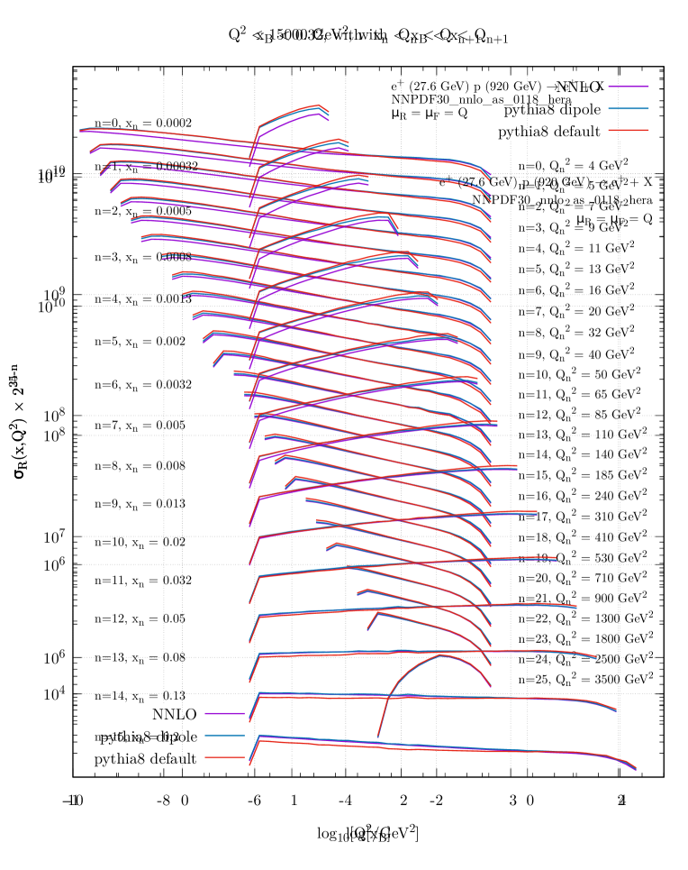
Figure 2: The reduced double differential cross section, defined in Eq. (28), binned in $x_{\mathchoice{\displaystyle}{\scriptstyle}{\scriptscriptstyle}{\scriptscriptstyle}\rm B}$ and plotted as a function of $\log{Q^{2}}$. For a given $n$ the lower bin-edge in $x_{\mathchoice{\displaystyle}{\scriptstyle}{\scriptscriptstyle}{\scriptscriptstyle}\rm B}$ is given by the printed $x_{n}$ and the upper limit is $x_{n+1}$. For the last bin with $n=16$ the upper edge is given by $x_{\mathchoice{\displaystyle}{\scriptstyle}{\scriptscriptstyle}{\scriptscriptstyle}\rm B}=0.5$. Note that in order to plot all curves in the same panel they have been multiplied by $2^{16-n}$. Plotted are fixed-order NNLO results (dark purple), POWHEG events showered with the dipole Pythia8 shower (blue), and POWHEG events showered with the default Pythia8 shower (red), both at parton level.

In Figs. 1 and 2 we show the reduced double differential cross section, as defined in Eq. (28). The results are either binned in $Q^{2}$ and plotted in $\log{x_{\mathchoice{\displaystyle}{\scriptstyle}{\scriptscriptstyle}{\scriptscriptstyle}\rm B}}$, or binned in $x_{\mathchoice{\displaystyle}{\scriptstyle}{\scriptscriptstyle}{\scriptscriptstyle}\rm B}$ and plotted in $\log{Q^{2}}$, where $Q$ is measured in GeV. In particular, we compare our NLO+PS result to an NNLO calculation obtained with disorder disorder that uses the DIS structure function branch of HOPPET Salam:2008qg which was developed in the context of the proVBFH programs Cacciari:2015jma ; Dreyer:2016oyx ; Dreyer:2018qbw ; Dreyer:2018rfu and uses the NNLO DIS coefficient functions computed in Refs. vanNeerven:1999ca ; vanNeerven:2000uj . We obtain NLO+PS results using two different versions of the Pythia8 showers Sjostrand:2014zea , namely the default Pythia8 and the dipole like Pythia8 shower introduced in Ref. Cabouat:2017rzi . For the purposes of the comparison in this section, the main difference between the two is that the default shower does not preserve the lepton kinematics, whereas the dipole variant does. In these plots we only run the shower phase of Pythia8, i.e. we do not include hadronisation and underlying event simulation. More details on the matching procedure with Pythia8 are given in App. C. As explained in Sec. 2, our POWHEG BOX implementation is constructed such that the radiation mappings preserve the underlying DIS kinematics, i.e. the lepton kinematics. For this reason the reduced cross sections obtained at pure NLO and at the level of the unshowered Les Houches Event (LHE) Alioli:2013nda file are in perfect agreement, i.e. there are no spurious higher-order terms induced by the POWHEG Sudakov for this observable. We note that this would not have been the case if our mappings did not preserve the DIS kinematics. Furthermore, with a parton shower which preserves the DIS invariants, such as the dipole Pythia8 shower Cabouat:2017rzi , the reduced cross-sections after parton shower are also identical. For this reason in Figs. 1 and 2 we do not show explicitly the NLO and LHE curves, as they are almost identical to the dipole (POWHEG+)Pythia8 shower results. On the other hand, the default Pythia8 shower does not preserve the DIS kinematics, and therefore one can expect modifications from the shower to the reduced cross sections, as is evident from Figs. 1 and 2, even though the hardest emission event generated by POWHEG does preserve the DIS kinematics. In particular, there are significant deviations for larger values of $x_{\mathchoice{\displaystyle}{\scriptstyle}{\scriptscriptstyle}{\scriptscriptstyle}\rm B}$ together with small to moderate values of $Q^{2}$. It is interesting to note that in this kinematic region the NNLO prediction is very close to the dipole Pythia8 prediction (i.e. it is very close to the NLO result), and hence true NNLO corrections are tiny in these regions. The discrepancies between the two Pythia8 showers can therefore be seen as spurious effects. This was already pointed out in Ref. Cabouat:2017rzi where it was found that the dipole Pythia8 shower correctly reproduces the singular limits of LO DIS matrix elements, whereas the default Pythia8 shower does not.

Figure 3: Ratios for the reduced cross section in Eq. (28) of NNLO (purple), Pythia8 dipole (blue), and Pythia8 default (red) both at parton level to NLO (black) for the bin $4\,\mathrm{GeV}^{2}<Q^{2}<5\,\mathrm{GeV}^{2}$ as a function of $\log{x_{\mathchoice{\displaystyle}{\scriptstyle}{\scriptscriptstyle}{\scriptscriptstyle}\rm B}}$ (left) and the same ratios for the bin $0.0002<x_{\mathchoice{\displaystyle}{\scriptstyle}{\scriptscriptstyle}{\scriptscriptstyle}\rm B}<0.00032$ as a function of $\log_{10}{Q^{2}}$ (right). The bands represent the 7-point scale variation of $\mu_{R}$ and $\mu_{F}$ by a factor of two around the central value $Q$.

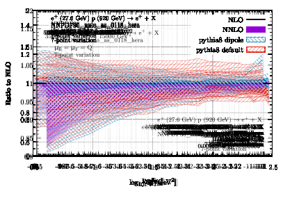
Figure 4: Same as Fig. 3, but for the bin $85\,\mathrm{GeV}^{2}<Q^{2}<110\,\mathrm{GeV}^{2}$ as a function of $\log{x_{\mathchoice{\displaystyle}{\scriptstyle}{\scriptscriptstyle}{\scriptscriptstyle}\rm B}}$ (left) and for the bin $0.0032<x_{\mathchoice{\displaystyle}{\scriptstyle}{\scriptscriptstyle}{\scriptscriptstyle}\rm B}<0.005$ as a function of $\log_{10}{Q^{2}}$ (right).

Figure 5: Same as Fig. 3, but for the bin $3500\,\mathrm{GeV}^{2}<Q^{2}<15000\,\mathrm{GeV}^{2}$ as a function of $\log{x_{\mathchoice{\displaystyle}{\scriptstyle}{\scriptscriptstyle}{\scriptscriptstyle}\rm B}}$ (left) and for the bin $0.08<x_{\mathchoice{\displaystyle}{\scriptstyle}{\scriptscriptstyle}{\scriptscriptstyle}\rm B}<0.13$ as a function of $\log_{10}{Q^{2}}$ (right).

To make the effect more visible, we select a few representative bins from the above two figures, and plot the ratios of the various predictions to the respective fixed-order NLO results in Figs. 3-5. Here it can be seen very clearly that for large values of $x_{\mathchoice{\displaystyle}{\scriptstyle}{\scriptscriptstyle}{\scriptscriptstyle}\rm B}$ there is a discrepancy between the two Pythia8 showers which is not accounted for by scale variations or true NNLO corrections. We do not include the scale variation band for the reference NLO prediction, as it is near identical to the band obtained with the Pythia8 dipole shower.

3.1.1 Impact of alternative momentum mappings

While the above discussion clearly demonstrates that our POWHEG implementation achieves NLO accuracy for inclusive quantities, it is instructive to explore how an implementation using mappings closer to the standard POWHEG BOX mappings would look like. The main kinematical difference between hadron-hadron collisions and DIS is that the incoming lepton momentum in DIS is fixed, whereas the incoming partons in a hadronic collision are sampled in their energy fractions. In order to simulate DIS it is therefore necessary that the mappings used by POWHEG preserve the incoming lepton momentum. The standard FSR mapping in POWHEG already does this, as it preserves both $x_{1}$ and $x_{2}$ (but we stress that these mappings do not preserve the DIS variables). In contrast, the ISR mappings modify both $x_{1}$ and $x_{2}$.

It is, however, straightforward to adapt the ISR mapping such that it only modifies the incoming parton momentum, but leaves the incoming lepton untouched. The minimally modified POWHEG map for ISR can be straightforwardly obtained by applying an additional longitudinal boost along the direction of the incoming electron, in order to restore its original value of the energy, to the kinematic reconstruction detailed in Sec. 5.1.1 of Ref. Frixione:2007vw . This boost changes the value of the $x$ fraction associated with the incoming parton, that, at variance with Eq. (5.7) of Ref. Frixione:2007vw , now becomes $x=\frac{\bar{x}}{1-\xi}$, but does not alter the values of the variable $\xi$, $y$ and $\phi$, which are defined in the partonic centre-of-mass frame. The only other necessary modifications are then the expression for upper bound for $\xi$, which now becomes $\xi<\bar{x}_{2}$, and for $\kappa_{t}^{\mathchoice{\displaystyle}{\scriptstyle}{\scriptscriptstyle}{\scriptscriptstyle}\rm ISR}$, which is now bounded by $\frac{S-\bar{s}}{4\sqrt{S}}$, being $\sqrt{S}$ the total hadronic centre-of-mass energy, and $\sqrt{\bar{s}}$ the underlying-Born centre-of-mass energy, which coincides with the mass of the recoiling system. However, with this minimally modified mapping, the outgoing lepton still takes recoil and hence the DIS variables are not conserved.

Figure 6: Similar to Fig. 1, but showing the minimally modified momentum mappings that do not preserve DIS kinematics in red. We do not show the default Pythia8 here.

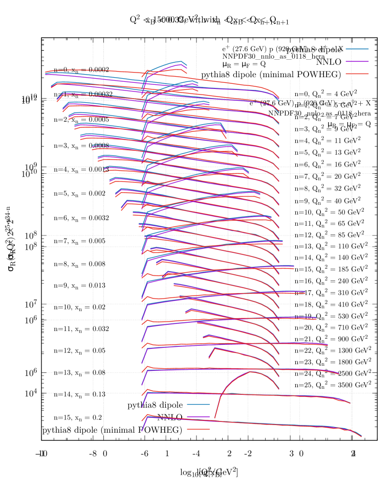
Figure 7: Similar to Fig. 2, but showing the minimally modified momentum mappings that do not preserve DIS kinematics in red. We do not show the default Pythia8 here.

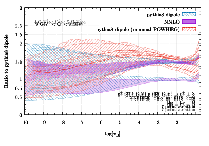
Figure 8: Similar to Fig. 3, but showing the minimally modified momentum mappings that do not preserve DIS kinematics in red. We do not show the default Pythia8 here and we normalise to our default “pythia8 dipole” result here in blue.

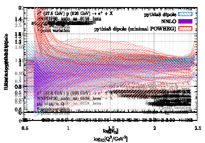
Figure 9: Similar to Fig. 4, but showing the minimally modified momentum mappings that do not preserve DIS kinematics in red. We do not show the default Pythia8 here and we normalise to our default “pythia8 dipole” result here in blue.

Figure 10: Similar to Fig. 5, but showing the minimally modified momentum mappings that do not preserve DIS kinematics in red. We do not show the default Pythia8 here and we normalise to our default “pythia8 dipole” result here in blue.

In Figs. 6-10 we show plots similar to the above, but now we use the minimally modified momentum mappings (red lines, labelled “minimal POWHEG” in the plots). For reference we show the POWHEG+Pythia8 dipole prediction (blue), using our new mappings from the above plots, as well as NNLO results (purple). As can be seen clearly, the predictions obtained with these minimally modified mappings exhibit sizable differences compared to the new mappings for inclusive quantities. In particular, we observe very large deviations for small $Q$ and $x_{\mathchoice{\displaystyle}{\scriptstyle}{\scriptscriptstyle}{\scriptscriptstyle}\rm B}$. It can also be seen that the deviations do not approximate the true NNLO corrections well.

It is interesting to note that LHC processes involving the exchange of colourless particles in the $t$-channel, like vector boson fusion (VBF) and single top production, which have been implemented in the POWHEG BOX in Refs. Nason:2009ai ; Jager:2012xk ; Alioli:2009je ; Frederix:2012dh , exhibit kinematics that are essentially double-DIS like. For this reason one would expect that these processes could benefit from a different momentum mapping. For instance, for VBF, it was observed in Ref. Cacciari:2015jma that the description of the rapidity separation between the two hardest jets as predicted with POWHEG has a very different shape compared to both NLO and NNLO predictions. It would be interesting to see if this tension can be resolved with our new mappings. We leave this question for future work.

3.2 Exclusive observables and comparison with resummation

In addition to the inclusive cross section considered above, information on the physics of DIS reactions can be gained from exclusive observables. In order to explore the complementarity of fixed-order perturbative calculations, resummed predictions and NLO+PS simulations, we performed a comparison of these approaches for two event shape variables. Following the Breit-frame definition of event shapes employed in the experimental analyses, we can distinguish between the remnant and current hemisphere, where particles in the remnant (current) hemisphere have positive (negative) pseudo-rapidities when the incoming photon has negative rapidity. Event shapes are formulated only in terms of particles in the current hemisphere. In particular, in this section we consider the thrust distribution $\tau_{\rm z,Q}$ and broadening $B_{\rm z,E}$, which are defined as

$$\tau_{\rm z,Q}=1-\frac{\sum_{h}2|\vec{p}_{z,h}|}{Q}\,,$$ (29)

$$B_{\rm z,E}=\frac{\sum_{h}|\vec{p}_{T,h}|}{2\sum_{h}|\vec{p}_{h}|},$$ (30)

where the momenta are defined in the Breit frame, the photon three-momentum determines the $z$-direction, and $h$ denotes all the hadrons in the current hemisphere. These observables are continuously-global and we can obtain resummed predictions at NLL accuracy, e.g. from CAESAR Banfi:2004yd , according to the practical details in section 3.2 of Ref. Banfi:2010xy . In particular, the matching of resummation and fixed order is performed with the mod-R scheme defined in that same reference.

Fig. 11

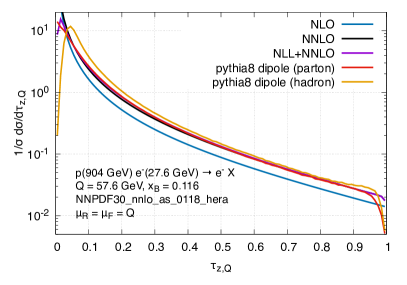
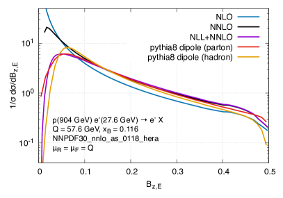
Figure 11: Thrust distribution normalised with respect to $Q$ (left) and broadening (right) for $Q=57.6$ GeV, $x_{\mathchoice{\displaystyle}{\scriptstyle}{\scriptscriptstyle}{\scriptscriptstyle}\rm B}=0.116$ for the photon-exchange contribution to $e^{-}p\rightarrow e^{-}X$ at NLO (blue), NNLO (black), NNLO+NLL (magenta), NLO+Pythia8 without (red) and with non-perturbative effects (orange).

depicts $\tau_{\rm z,Q}$ and $B_{z,E}$ for the photon-exchange contribution to $e^{-}p\rightarrow e^{-}X$ with $E_{p}=904.5$ GeV, $E_{e}=27.6$ GeV. We consider fixed-underlying Born kinematics, corresponding to $x_{\mathchoice{\displaystyle}{\scriptstyle}{\scriptscriptstyle}{\scriptscriptstyle}\rm B}=0.116$ and $Q=57.6$ GeV. These settings correspond to the average values of $x_{\mathchoice{\displaystyle}{\scriptstyle}{\scriptscriptstyle}{\scriptscriptstyle}\rm B}$, $Q$ and $\sqrt{s}=316$ GeV reported by the experimental analysis of Ref. H1:2005zsk for the bin $50\text{~{}GeV}<Q<70\text{~{}GeV}$. Notice that this value of $Q$ ensures that mass effects, which are included in the PS simulation, but not in the NNLO+NLL prediction and in the POWHEG underlying calculation, are negligible.

Furthermore, an event is included, if the sum over the energies $E_{h}$ of all hadronic objects $h$ in the current hemisphere exceeds a minimum value $\epsilon_{\mathrm{lim}}$,

$$E_{\mathrm{curr}}=\sum_{h}E_{h}>\epsilon_{\mathrm{lim}}=Q/10\,.$$ (31)

As discussed in Ref. Antonelli:1999bv , starting from order $\alpha_{s}^{2}$ there can be configurations where the current hemisphere is populated only by soft large-angle radiation from partons in the remnant hemisphere. It is then necessary to introduce a cut on $E_{\mathrm{curr}}$ to remove sensitivity to these soft emissions in event shapes normalised with respect to $E_{\mathrm{curr}}$ (or to $\sum_{h}|\vec{p}_{z,h}|$), that would be otherwise infrared unsafe.

In the parton-level Pythia8 curve, we dress POWHEG events with the QCD Pythia8 dipole shower. In the hadron-level curve we also include hadronisation and beam remnants effects. The fixed-order predictions are obtained with DISENT Catani:1996vz . Since the event shapes shown here vanish at Born-level, the predictions shown here are effectively LO and NLO accurate even though we label the predictions by their inclusive accuracy, i.e. NLO and NNLO.

At NLO, the distributions steeply increase towards small values. This behaviour reflects the distinguished kinematics of a LO DIS configuration with exactly one final-state parton, which at NLO can only be altered by the emission of a single additional parton. One more parton can arise at NNLO where we observe a peak at small values of $\tau_{\rm z,Q}$ and $B_{z,E}$, which is due to the distributions turning negative (and diverging) due to large negative virtual corrections.

The divergences of the fixed-order calculations are removed by the resummation of all-order leading (and next-to-leading) logarithmically enhanced terms. In the NLO+PS results the parton shower has a similar effect.

We note that, away from the divergence, our POWHEG prediction is much closer to NNLO than to NLO at the parton level, indicating that higher order terms induced by the shower and matching approximate well the true NNLO corrections.

We also notice that, while for the broadening distribution (right panel), both the NLO+PS (parton) and the NNLO+NLL curves are peaked around the same value of $B_{\rm z,E}$. For $\tau_{z,Q}$ (left panel), the NNLO+NLL Sudakov peak is at a much lower value (i.e. $\tau_{z,Q}\lesssim 0.02$) and it is not visible in the parton shower predictions because of the PS cutoff $\mu_{\min}\approx 0.5$ GeV.

Hadronisation effects are sizable for small values of the event shapes. In case of the thrust distribution, they correspond to a roughly constant shift, while for the broadening this shift depends on the value of $B_{\rm z,E}$.

3.3 Jet and VBF related observables

Figure 12: The hardest anti-$k_{T}$ $R=0.4$ jet in the rapidity window $-4.5<\eta^{\mathrm{jet}}<-1.5$ for events satisfying the cuts of Eq. (32). We show LO (blue), NLO (grey), NNLO (purple), our new DIS implementation showered with Pythia8 (red) and the minimally modified POWHEG implementation with the same shower (orange). On the right we show the ratio to the NLO prediction. The bands correspond to a 7-point scale variation around the central scale $\mu=Q$.

Figure 13: Same as Fig. 12, but now showing the rapidity of the hardest jet satisfying $p_{T}^{\mathrm{jet}}>30\,\mathrm{GeV}$.

Although the full implementation and study of VBF or single top production is beyond the scope of this paper, it is possible to mimic the kinematics of jets produced in these processes at the LHC. As discussed above, our POWHEG BOX implementation reproduces the DIS structure functions exactly at NLO since the momentum mappings preserve the DIS variables, or equivalently they leave the lepton momenta untouched. However, if we instead turn to the kinematics of the DIS jet, we see that it is clearly modified by the extra radiation. The POWHEG method still guarantees that we describe the hardest jet with NLO accuracy, but with higher-order terms in $\alpha_{s}$ induced by the POWHEG Sudakov form factor (and the subsequent showering).

Typical VBF analyses at the LHC look for two well-separated jets with a large invariant mass. Therefore, to mimic VBF like topologies, we produce events in proton-electron collisions, with a proton energy of $6500\,\mathrm{GeV}$ and an electron energy of $300\,\mathrm{GeV}$. Additionally we require that

$$30\,\mathrm{GeV}<Q<120\,\mathrm{GeV},\quad 0.04<x_{\mathchoice{\displaystyle}{\scriptstyle}{\scriptscriptstyle}{\scriptscriptstyle}\rm B},\quad p_{T}^{\mathrm{lep}}>30\,\mathrm{GeV}.$$ (32)

The cut on $x_{\mathchoice{\displaystyle}{\scriptstyle}{\scriptscriptstyle}{\scriptscriptstyle}\rm B}$ ensures a large invariant mass of the colliding system, and the range in $Q$ is close to the typical momentum transfer in VBF of the order of the $W$ mass. We also only include photon-mediated DIS to allow for a comparison with a fixed order code.

We cluster the events in the laboratory frame with the anti-$k_{T}$ algorithm Cacciari:2008gp with $R=0.4$ using FastJet v3.4.0 Cacciari:2011ma . We then look for the jet of hardest transverse momentum with pseudo-rapidity $-4.5<\eta^{\mathrm{jet}}<-1.5$ (the incoming parton is in the minus $z$-direction). We require this jet to have $p_{T}^{\mathrm{jet}}>30\,\mathrm{GeV}$. We stress that these quantities are defined in the lab frame, not in the Breit frame, hence they are non-vanishing already at LO.

In Figs. 12-13 we show the transverse momentum and the rapidity, respectively, of the hardest jet. In addition to our new POWHEG implementation (shown in red) we also show fixed-order predictions up to NNLO and events generated with the minimal POWHEG implementation described in the previous section (orange). We use the Pythia8 dipole shower to shower both sets of POWHEG events. The bands are obtained through the usual 7-point scale variation around the central scales $\mu_{R/F}=Q$. In App. E we show results obtained using two different central scales, which lead to similar findings to the ones presented here.

The fixed order predictions are obtained with the program disorder disorder which uses DISENT Catani:1996vz and the projection-to-Born method Cacciari:2015jma together with the NNLO DIS coefficient functions vanNeerven:1999ca ; vanNeerven:2000uj as implemented in the DIS structure function branch of HOPPET Salam:2008qg .

We note that the minimal POWHEG implementation is typically further away from the fixed order NLO curve than the new implementation presented here. The differences between the two POWHEG generators are, however, compatible in size with the scale uncertainty band, although the true NNLO corrections (in purple) tend to favour our new POWHEG implementation. It will be interesting to see if this pattern persists if one were to use our new mappings in VBF production or single top.

The size of the scale variation in both POWHEG implementations deserves some comments. Naively one would expect the scale variation bands to be commensurate in size with those of the NLO calculation. However, in POWHEG when one varies the renormalisation and factorisation scales this only impacts the $\bar{B}$ function. The scale at which $\alpha_{s}$ is evaluated in the Sudakov form factor remains the same (the transverse momentum of the emission). The $\bar{B}$ function, introduced in Sec. 2.2.1, is essentially the NLO inclusive cross section, which has tiny scale variations for the values of $Q$ probed here. As a consequence the scale variation is dramatically underestimated – even more than in the fixed order prediction. In App. D we study this effect in more detail. Although the scale variation band is always underestimated compared to the fixed order NLO band, including more damping can ameliorate this effect somewhat.

4 Phenomenological studies

Figure 14: Thrust distribution (left) and broadening (right) for different bins in $Q$, at the hadron level for the dipole (red), and Vincia (blue) showers, and at the parton level (i.e. without hadronisation and beam-remnant effects) for the dipole shower (magenta), together with the H1 data of Ref. H1:2005zsk . For a given $Q$-bin $n$, the average value of $Q$ is denoted by $\langle Q_{n}\rangle$, and the corresponding curve is multiplied by a factor of $50^{2(6-n)}$ for better readability.

In this section we present hadron-level predictions for the HERA and EIC experiments. In particular, we interface our NLO+PS generator with Pythia8 Bierlich:2022pfr , which also provides hadronisation and beam-remnant effects. The hadron-level predictions are obtained considering both the dipole shower Cabouat:2017rzi , which we have employed in the previous section, as well as the Pythia8 implementation of the default antenna Vincia shower Brooks:2020upa . We do not include QED radiation or hadron-decay effects.

4.1 Comparison to HERA data

We now compare predictions obtained with our new POWHEG BOX implementation with HERA data analyzed by the H1 Collaboration in Ref. H1:2005zsk corresponding to an integrated luminosity of $\mathcal{L}_{\mathrm{int}}=106$ pb^-1. Following their study, we consider collisions of electrons or positrons of energy $E_{e}=27.6$ GeV and protons of energy $E_{p}=820$ GeV or $E_{p}=920$ GeV resulting in centre-of-mass energies $\sqrt{s}$ of 301 GeV and 319 GeV, respectively. Electron and positron samples are generated independently and combined in the results discussed below corresponding to the composition of the data sample of Ref. H1:2005zsk , i.e. $e^{+}p$: $\sqrt{s}=301$ GeV, $\mathcal{L}_{\mathrm{int}}=30~{}$pb^-1; $e^{-}p$: $\sqrt{s}=319$ GeV, $\mathcal{L}_{\mathrm{int}}=14~{}$pb^-1; $e^{+}p$: $\sqrt{s}=319$ GeV, $\mathcal{L}_{\mathrm{int}}=62~{}$pb^-1.

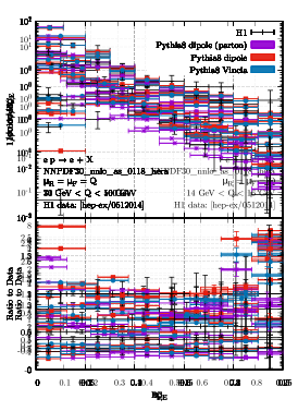
Figure 15: Thrust distribution at the hadron level for the dipole (red), and Vincia (blue) showers, and at the parton level (i.e. without hadronisation and beam-remnant effects) for the dipole shower (magenta), together with the H1 data of H1:2005zsk , for the bins $14~{}\text{GeV}<Q<16$ GeV (left), $30~{}\text{GeV}<Q<50$ GeV (middle), and $70~{}\text{GeV}<Q<100$ GeV (right). The bands represent the 7-point scale variation of $\mu_{R}$ and $\mu_{F}$ by a factor of two around the central value $Q$ for the POWHEGresults. The lower panels show the ratio of the predictions to data.

We use the NNPDF30_nnlo_as_0118_hera set already mentioned in Sec. 3. Only events in the range

$$14~{}\text{GeV}<Q<200~{}\text{GeV}\,,$$

$$0.1<y_{\mathchoice{\displaystyle}{\scriptstyle}{\scriptscriptstyle}{\scriptscriptstyle}\rm DIS}<0.7\,,$$ (33)

are taken into account. Furthermore, following the H1 analysis, we accept events where the energy in the current hemisphere exceeds a minimum value $\epsilon_{\mathrm{lim}}$, according to Eq. (31). As discussed in Sec. 3.2, this cutoff ensures the collinear and infrared safety of event shapes which are normalised with respect to $E_{\mathrm{curr}}$ (or $\sum_{h}|\vec{p}_{z,h}|$), by removing events with no hard, but only arbitrarily soft partons in the current hemisphere.

Event shape variables constitute a class of quantities particularly suited to probe the interplay of the hard scattering and the hadronisation mechanism governing DIS processes (see e.g. Ref. Dasgupta:2003iq ). Following Ref. H1:2005zsk , we introduce the thrust variable $\tau_{\rm z,E}$ is defined by

$$\tau_{\rm z,E}=1-T_{\rm z,E}\quad\text{with}\quad T_{\rm z,E}=\frac{\sum_{h}|\vec{p}_{z,h}|}{\sum_{h}|\vec{p}_{h}|}\,,$$ (34)

where the summations run over all hadronic objects $h$ in the current hemisphere, $\vec{p}_{h}$ denotes the Breit-frame three-momentum of parton $h$ and $\vec{p}_{z,h}$ its component along the $z$ axis, which is chosen along the direction of the virtual boson. The thrust variable is a measure of the momentum components of the hadronic system parallel to the $z$ axis in the Breit frame. For the broadening we use the definition of Eq. (30).

In Fig. 14 we show $\tau_{\rm z,E}$ and $B_{\rm z,E}$, respectively, for various $Q$ bins at the same time, together with the H1 data of H1:2005zsk . To assess the impact of soft-physics effects, we also produce parton-level predictions in which hadronisation and beam-remnant effects are not included. We do so only for the dipole shower, as the modelling of these effects is the same for Vincia predictions. In Figs. 15 and 16 we consider the same event shapes for selected ranges of $Q$ together with the 7-point variation of $\mu_{R}$ and $\mu_{F}$.

Figure 16: Same as Fig. 15, but for the broadening distribution.

We select the lowest $Q$-bin, $14~{}\text{GeV}<Q<16$ GeV, which is dominated by photon exchange contributions, one with intermediate values of $Q$, and one including the value where $Q$ coincides with the mass of the $Z$ boson.

For $\tau_{\rm z,E}$ we find good agreement of our hadron-level predictions with H1 data. Especially at low values of $Q$ hadronisation effects are crucial for a reasonable description of data. As expected, at higher values of $Q$ the impact of these effects becomes less relevant. While agreement between predictions and data is generally worse for the broadening, a similar trend as in the thrust distribution can be observed, with hadronisation effects being particularly important at low values of $Q$ and differences between the dipole and the antenna showers being small throughout. Scale uncertainties are generally small for both distributions, but largest towards their respective upper ends, which reflects the relevance of higher-order corrections in these kinematic regions. The smallness of the scale variation in these plots can mostly be attributed to the fact that the plots show normalised distributions.

Similarly to the event shapes of Eqs. (34) and (30), the squared jet mass $\rho$ and the $C$-parameter are defined as

$$\rho=\frac{\left(\sum_{h}E_{h}\right)^{2}-\left(\sum_{h}\vec{p}_{h}\right)^{2}}{\left(2\sum_{h}|\vec{p}_{h}|\right)^{2}}\,,$$ (35)

and

$$C=\frac{3}{2}\frac{\sum_{h,h^{\prime}}|\vec{p}_{h}||\vec{p}_{h^{\prime}}|\cos^{2}\theta_{hh^{\prime}}}{\left(\sum_{h}|\vec{p}_{h}|\right)^{2}}\,,$$ (36)

where $h$ and $h^{\prime}$ are two different hadronic objects in the current hemisphere separated by an angle $\theta_{hh^{\prime}}$. In Fig 17

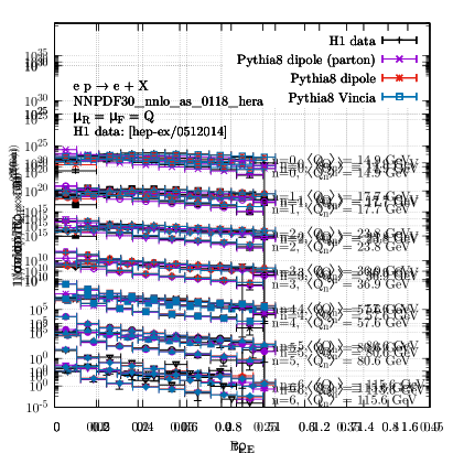
Figure 17: Same as Fig. 14, but for the squared jet mass (left) and the $C$-parameter (right).

we show $\rho$ and $C$ for various $Q$ bins at the same time.

Figure 18: Same as Fig. 15, but for the squared jet mass.

Figure 19: Same as Fig. 15, but for the $C$-parameter distribution.

Figs. 18 and 19 depict the same distributions for selected bins in $Q$ together with scale uncertainty bands. For $\rho$ and $C$ we observe a similar pattern as in the case of thrust and broadening. Taking hadronisation effects into account is crucial for a reasonable agreement between simulation and data. Even after the inclusion of hadronisation effects, at low values of $Q$ our predictions for both distributions deviate from data. Better agreement is found at intermediate values of $Q$. At large values of $Q$ for most bins predictions agree with data considering the large statistical uncertainties of the latter.

We note that a large impact of non-perturbative effects has also been reported in Knobbe:2023ehi for the so-called 1-jettiness distribution which is closely related to the thrust distribution.

4.2 Predictions for the EIC

After employing our new POWHEG BOX implementation for the description of H1 legacy results, we turn to DIS at the future EIC. We consider electron-proton collisions with $E_{e}=18$ GeV, $E_{p}=275$ GeV, both in the neutral current (NC) and charged current (CC) modes with the incoming lepton either remaining intact or being converted into a neutrino.

Following Ref. Borsa:2022cap , the DIS kinematics are restricted by

$$25~{}\text{GeV}^{2}<Q^{2}<1000~{}\text{GeV}^{2}\,,$$

$$0.04<y_{\mathchoice{\displaystyle}{\scriptstyle}{\scriptscriptstyle}{\scriptscriptstyle}\rm DIS}<0.95\,.$$ (37)

In contrast to the settings used in the HERA analysis of Sec. 4.1, for our EIC predictions we employ the PDF4LHC15_nlo_100_pdfas parton distribution set Butterworth:2015oua to account for LHC constraints on the proton structure. Jets are reconstructed in the laboratory frame with the anti-$k_{T}$ algorithm Cacciari:2008gp using an $R$-parameter of $R=0.8$ and restrictions on transverse momentum and pseudorapidity,

$$p_{T}^{\mathrm{jet}}>5~{}\text{GeV}\,,\quad|\eta^{\mathrm{jet}}|<3\,.$$ (38)

Fig. 20

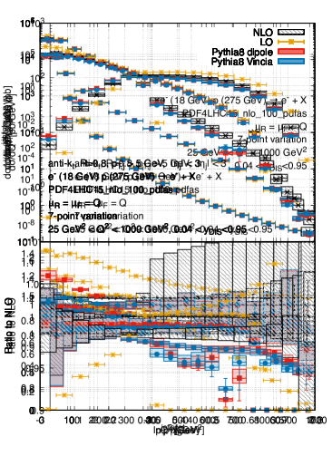
Figure 20: Distributions of $Q^{2}$ (left) and $x_{\mathchoice{\displaystyle}{\scriptstyle}{\scriptscriptstyle}{\scriptscriptstyle}\rm B}$ (right) for NC DIS at the EIC with $\sqrt{s}=140$ GeV and within the cuts of Eq. (4.2) at LO (orange), NLO (magenta), and NLO+PS results, obtained with dipole shower (red) or Vincia (blue) Pythia8 showers. Hadronisation and beam remnant effects are included in the NLO+PS simulations. Error bars indicate statistical uncertainties, bands are obtained by a 7-point scale variation of $\mu_{R}$ and $\mu_{F}$ by a factor of two around the central value $Q$. The lower panels display the ratios to the respective NLO results.

displays the $Q^{2}$ and $x_{\mathchoice{\displaystyle}{\scriptstyle}{\scriptscriptstyle}{\scriptscriptstyle}\rm B}$ distributions of the NC cross section within the cuts of Eq. (4.2) at LO, NLO, and NLO+PS accuracy (with the inclusion of hadronisation and beam remnant effects) for two different shower versions. The NLO corrections change the LO results in a non-uniform way, slightly shifting the $Q^{2}$ distribution to larger values. Also the shape of the $x_{\mathchoice{\displaystyle}{\scriptstyle}{\scriptscriptstyle}{\scriptscriptstyle}\rm B}$ distribution is modified by NLO corrections with a tendency to smaller $x_{\mathchoice{\displaystyle}{\scriptstyle}{\scriptscriptstyle}{\scriptscriptstyle}\rm B}$ values at LO. Both the Vincia and the dipole showers preserve the lepton kinematics, hence the NLO+PS results agree with the NLO result. For the NLO+PS results, we also performed a 7-point scale variation, modifying the renormalisation and factorisation scales independently by factors of two around their central value $Q$.

In Fig. 21

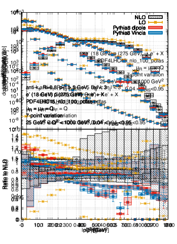
Figure 21: Distributions of $p_{T}^{\mathrm{jet}}$ (left) and $\eta^{\mathrm{jet}}$ (right) for NC DIS at the EIC with $\sqrt{s}=140$ GeV and within the cuts of Eqs. (38)–(4.2).

we display the transverse-momentum and pseudorapidity distributions of the hardest jet reconstructed with cuts of Eqs. (38)–(4.2). We remind the reader that these quantities are defined in the lab frame, hence they are non-vanishing already at LO. At LO, the accessible range of transverse momentum is limited by the upper limit on $Q^{2}$ of 1000 GeV², $p_{T}^{\mathrm{jet}}<Q\sim 32$ GeV. Beyond LO, the transverse momentum available for the hadronic system can instead be distributed among various final-state partons resulting in non-vanishing contributions to the respective cross sections beyond this threshold. Here NLO predictions are effectively leading order accurate, which is reflected by the larger scale uncertainly bands. We observe that the NLO corrections considerably reduce the $p_{T}^{\mathrm{jet}}$ distribution at low values, and the parton shower slightly enhances that effect. The shape of the pseudorapidity distribution is modified by NLO corrections in an asymmetric way with largest effects at high values of $|\eta^{\mathrm{jet}}|$. In this range an additional, though smaller shape distortion is caused by the parton shower. The impact of the shower is large in kinematic regions that are not accessible at LO, but require the presence of additional radiation, such as the large transverse-momentum region, or for very negative values of $\eta^{\mathrm{jet}}$. In particular, we find that the dipole and the Vincia shower agree remarkably well with each other, except for $\eta^{\mathrm{jet}}\lesssim-2$, where differences between the two shower models reach 10-15$\%$. Scale uncertainties are generally smaller than differences between fixed-order and NLO+PS results.

We now consider the CC case. The main difference between the NC and the CC processes is that the former can proceed via the exchange of a virtual photon or a $Z$ boson between the scattering electron and proton, and so is divergent for small $Q^{2}$ or $p_{T}^{\mathrm{jet}}$ values, while the CC cross section is entirely due to weak boson exchange contributions, which leads to a finite cross section also for vanishing $Q^{2}$. Nonetheless, in the most characteristic distributions, radiative corrections display similar features as in the NC case. The $Q^{2}$ and $x_{\mathchoice{\displaystyle}{\scriptstyle}{\scriptscriptstyle}{\scriptscriptstyle}\rm B}$ distributions depicted in Fig. 22

Figure 22: Same as Fig. 20, but for the charged current channel.

exhibit negative NLO corrections of about 5% to 10% over the entire range of $Q^{2}$. At small values of $x_{\mathchoice{\displaystyle}{\scriptstyle}{\scriptscriptstyle}{\scriptscriptstyle}\rm B}$ the NLO corrections are small and negative, while they become positive beyond $x_{\mathchoice{\displaystyle}{\scriptstyle}{\scriptscriptstyle}{\scriptscriptstyle}\rm B}\approx 0.3$ and reach values of almost 25% at large $x_{\mathchoice{\displaystyle}{\scriptstyle}{\scriptscriptstyle}{\scriptscriptstyle}\rm B}$. Parton-shower effects are small in each case.

The transverse-momentum and pseudorapidity distributions illustrated in Fig. 23

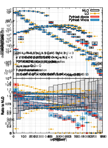
Figure 23: Same as Fig. 21, but for the charged current channel.

turn out to be less sensitive to NLO corrections at low $p_{T}^{\mathrm{jet}}$ in the CC than in the NC case, but receive small negative NLO corrections at intermediate transverse momenta. The different behaviour of this jet distribution at low $p_{T}^{\mathrm{jet}}$ can be traced back to the presence of photon-exchange contributions in the NC case. The pseudorapidity distribution, which is most sensitive to perturbative corrections at large values of $|\eta^{\mathrm{jet}}|$ where the cross section itself is small, exhibits a similar behaviour as in the NC case.

5 Summary and conclusions

In this paper we have presented the first implementation of an NLO+PS event generator for DIS in the POWHEG BOX. The code will be made publically available there. While the POWHEG BOX allows for almost automated generation of hadron-hadron collisions, the kinematics of the DIS process required us to address a number of problems.

In particular we had to modify the FKS momentum mappings that are used in the POWHEG BOX, in order to preserve both the incoming and outgoing lepton momenta. The standard ISR map in the POWHEG BOX is such that it modifies the kinematics of both the incoming legs. Although the FSR map does not modify the incoming energy fractions, it does not preserve the DIS variables, $x_{\mathchoice{\displaystyle}{\scriptstyle}{\scriptscriptstyle}{\scriptscriptstyle}\rm B}$, $y_{\mathchoice{\displaystyle}{\scriptstyle}{\scriptscriptstyle}{\scriptscriptstyle}\rm DIS}$, and $Q$. We have shown that if one makes only minimal modifications to these mappings, such that the ISR map conserves the incoming lepton momentum, but the FSR maps is untouched, the resulting POWHEG generator substantially modifies even very inclusive distributions, even outside the NLO scale uncertainty. On the other hand, with our new and significantly different mappings, which do preserve DIS kinematics, NLO accuracy is numerically retained. Since the momentum mapping introduced preserves the DIS variables, it is possible to be fully differential in $x_{\mathchoice{\displaystyle}{\scriptstyle}{\scriptscriptstyle}{\scriptscriptstyle}\rm B}$ and $Q^{2}$ or to consider specific ranges in $x_{\mathchoice{\displaystyle}{\scriptstyle}{\scriptscriptstyle}{\scriptscriptstyle}\rm B}$ and $Q^{2}$.

We have presented several phenomenological studies. Firstly, we compared our results to event-shape distributions measured by H1. Overall, we observe a reasonable agreement, but for certain event shapes, there are discrepancies between the shapes of our theoretical predictions and the data. This is not unexpected as event shapes are described only at LO+PS in our generator, starting at ${\cal O}(\alpha_{s})$. In the future, we plan to extend the description of DIS processes in POWHEG to include DIS + one jet. This extension would allow us to achieve NLO accuracy for both inclusive and one-jet quantities within the MINLO framework. By doing so, we aim to improve the precision and reliability of our predictions for a broader range of observables in DIS and in particular to achieve NLO accuracy both for inclusive and one-jet quantities.

We then considered a possible future setup at the future EIC. We find that NLO corrections can be important and must be included to have an accurate description of this process. This is the case both for the $Q^{2}$ and $x_{B}$ dependence of the inclusive cross section, as well as for the transverse momentum and rapidity distribution of the leading jet, where NLO corrections give rise to sizable shape difference compared to LO and parton shower effects are also important.

Although the present study focused on DIS, our work has implications also for LHC processes which involve the exchange of colourless particles in the $t$-channel like VBF and single top production. We leave it for future work to investigate the impact of the new momentum mappings in these processes. Very recently a family of NLL-accurate parton showers for DIS and VBF was presented in Ref. vanBeekveld:2023lfu . It will be also interesting in the future to investigate the matching of these showers to our POWHEG generator. Our code can be downloaded from the following SVN repository:

svn://powhegbox.mib.infn.it/trunk/User-Processes-RES/DIS

Appendix A Phase-space parameterisation

We consider the LO process $\ell(\bar{k}_{i}),q(\bar{p}_{i})\rightarrow\ell(\bar{k}_{f}),q(\bar{p}_{f})$. In the centre-of-mass frame, the momenta of the particles can be explicitly written as

$$\bar{k}_{i}= \frac{\sqrt{\bar{s}}}{2}\left(1,0,0,+1\right)$$ (39)

$$\bar{p}_{i}= \frac{\sqrt{\bar{s}}}{2}\left(1,0,0,-1\right)$$ (40)

$$\bar{k}_{f}= \frac{\sqrt{\bar{s}}}{2}\left(1,+\sin\bar{\phi}\sin\bar{\theta},+\cos\bar{\phi}\sin\bar{\theta},+\cos\bar{\theta}\right)$$ (41)

$$\bar{p}_{f}= \frac{\sqrt{\bar{s}}}{2}\left(1,-\sin\bar{\phi}\sin\bar{\theta},-\cos\bar{\phi}\sin\bar{\theta},-\cos\bar{\theta}\right),$$ (42)

where $\bar{s}=(\bar{k}_{i}+\bar{p}_{i})^{2}$ is the partonic centre-of-mass energy. Introducing $y_{\mathchoice{\displaystyle}{\scriptstyle}{\scriptscriptstyle}{\scriptscriptstyle}\rm DIS}=(1+\cos\bar{\theta})/2$ and $x_{\mathchoice{\displaystyle}{\scriptstyle}{\scriptscriptstyle}{\scriptscriptstyle}\rm B}=\bar{s}/S$, being $S=(P+\bar{k}_{i})^{2}$ and $P$ the incoming proton momentum, it is easy to see that the LO phase space can be written as

$$\int\differential\bar{\Phi}_{2}=\int\differential x\frac{\differential^{3}\mathbf{k}_{f}}{2k_{f}^{0}(2\pi)^{3}}\frac{\differential^{3}\mathbf{p}_{f}}{2p_{f}^{0}(2\pi)^{3}}(2\pi)^{4}\delta^{(4)}\quantity(k_{i}+p_{i}-k_{f}-p_{f})=\int\frac{\differential x\differential y_{\mathchoice{\displaystyle}{\scriptstyle}{\scriptscriptstyle}{\scriptscriptstyle}\rm DIS}\differential\bar{\phi}}{16\pi^{2}}.$$ (43)

If we consider the emission of an extra parton with momentum $p_{r}$, the phase space $\differential\Phi_{3}$ is given by

$$\int\differential\Phi_{3}=\int\differential x\,\differential\phi_{3}=\int\differential x\frac{\differential^{3}\mathbf{k}_{f}}{2k_{f}^{0}(2\pi)^{3}}\frac{\differential^{3}\mathbf{p}_{f}}{2p_{f}^{0}(2\pi)^{3}}\frac{\differential^{3}\mathbf{p}_{r}}{2p_{r}^{0}(2\pi)^{3}}(2\pi)^{4}\delta^{(4)}\quantity(k_{i}+p_{i}-k_{f}-p_{f}-p_{r}),$$ (44)

where $x$ is the longitudinal momentum fraction of the incoming parton and $\differential\phi_{3}$ is the final state three particle phase space. We use $p$ and $k$ to denote the recoiled momenta, while $\bar{p}$ and $\bar{k}$ are employed for the underlying Born kinematics. Bold-face notation is used for three-momenta.

Like for the LO case, in the partonic centre-of-mass frame we can write for the incoming partons

$$k_{i} =\frac{\sqrt{s}}{2}\quantity(1,0,0,+1)\,,$$ (45)

$$p_{i} =\frac{\sqrt{s}}{2}\quantity(1,0,0,-1)\,,$$ (46)

where $s=(k_{i}+p_{i})^{2}=xS$. The explicit parametrisation of the three final-state particles will differ in case of ISR and FSR.

A.1 Phase-space parameterisation for initial-state radiation

In order to evaluate the phase-space of Eq. (44) for the case of ISR we parameterisation the momentum of the radiated parton in terms of the FKS variables Frixione:1995ms $\xi,y$ and $\phi$, as

$$p_{r} =\xi\frac{\sqrt{s}}{2}\quantity(1,\sqrt{1-y^{2}}\cos\phi,\sqrt{1-y^{2}}\sin\phi,y)\,,$$ (47)

while the momentum of the final-state lepton reads

$$k_{f} =\xi_{k}\frac{\sqrt{s}}{2}\quantity(1,\sqrt{1-y_{k}^{2}}\cos\bar{\phi},\sqrt{1-y_{k}^{2}}\sin\bar{\phi},y_{k})\,.$$ (48)

Momentum conservation implies that the momentum of the other final-state parton is $p_{f}=p_{i}+k_{i}-p_{r}-k_{f}$. In terms of these variables one has $\differential^{3}\mathbf{p}_{r}=dp_{r}^{0}(p_{r}^{0})^{2}d\phi dy$ and $\differential^{3}\mathbf{k}_{f}=dk_{f}^{0}(k_{f}^{0})^{2}d\bar{\phi}dy_{k}$. After performing the integration over $\differential^{3}\mathbf{p}_{f}$ one obtains for the phase-space integral of Eq. (44)

$$\int\differential\Phi_{3} =\frac{1}{8(2\pi)^{5}}\int\differential x\;\differential k_{f}^{0}\;\differential\bar{\phi}\;\differential y_{k}\;\differential p_{r}^{0}\;\differential\phi\;\differential y\;\frac{k_{f}^{0}p_{r}^{0}}{p_{f}^{0}}\delta\quantity(k_{i}^{0}+p_{i}^{0}-k_{f}^{0}-p_{f}^{0}-p_{r}^{0}),$$ (49)

where the final-state parton’s energy is fixed to $p_{f}^{0}=\sqrt{\quantity(-\mathbf{k}_{f}-\mathbf{p}_{r})^{2}}$.

In terms of the DIS variables $y_{\mathchoice{\displaystyle}{\scriptstyle}{\scriptscriptstyle}{\scriptscriptstyle}\rm DIS}$, introduced in Eq. (1), and $Q^{2}=-(k_{i}-k_{f})^{2}$ one has

$$y_{k}=\frac{s(1-y_{\mathchoice{\displaystyle}{\scriptstyle}{\scriptscriptstyle}{\scriptscriptstyle}\rm DIS})-Q^{2}}{s(1-y_{\mathchoice{\displaystyle}{\scriptstyle}{\scriptscriptstyle}{\scriptscriptstyle}\rm DIS})+Q^{2}}\,,\quad k_{f}^{0}=\xi_{k}\frac{\sqrt{s}}{2}=\frac{s(1-y_{\mathchoice{\displaystyle}{\scriptstyle}{\scriptscriptstyle}{\scriptscriptstyle}\rm DIS})+Q^{2}}{2\sqrt{s}}\,,$$ (50)

and, thus,

$$\differential k_{f}^{0}\;\differential y_{k}=\differential y_{\mathchoice{\displaystyle}{\scriptstyle}{\scriptscriptstyle}{\scriptscriptstyle}\rm DIS}\;\differential Q^{2}\;\frac{1}{2k_{f}^{0}}\,.$$ (51)

The phase-space integral of Eq. (49) then becomes

$$\int\differential\Phi_{3} =\frac{1}{16(2\pi)^{5}}\int\differential x\;\differential y_{\mathchoice{\displaystyle}{\scriptstyle}{\scriptscriptstyle}{\scriptscriptstyle}\rm DIS}\;\differential\bar{\phi}\;\differential\lambda\;\differential\xi\;\differential\phi\;\differential y\;\frac{s\,y_{\mathchoice{\displaystyle}{\scriptstyle}{\scriptscriptstyle}{\scriptscriptstyle}\rm DIS}\,p_{r}^{0}}{p_{f}^{0}}\delta\quantity(k_{i}^{0}+p_{i}^{0}-k_{f}^{0}-p_{f}^{0}-p_{r}^{0})\,,$$ (52)

where $\lambda\equiv Q^{2}/(2k_{i}q)=Q^{2}/(sy_{\mathchoice{\displaystyle}{\scriptstyle}{\scriptscriptstyle}{\scriptscriptstyle}\rm DIS})=x_{B}/x$ and where $p_{r}^{0}$ and $p_{f}^{0}$ are given by

$$p_{r}^{0}=\xi\frac{\sqrt{s}}{2}\,,\qquad p_{f}^{0}=\frac{\sqrt{s}}{2}\sqrt{\xi^{2}+\xi_{k}^{2}+2\xi\xi_{k}yy_{k}+2\xi\xi_{k}\sqrt{1-y^{2}}\sqrt{1-y_{k}^{2}}\cos\left(\phi-\bar{\phi}\right)}\,,$$ (53)

with $\xi_{k}$ defined in Eq. (50). The integration bounds in Eq. (52) are given by

$$0<x,\lambda,\xi,y_{\mathchoice{\displaystyle}{\scriptstyle}{\scriptscriptstyle}{\scriptscriptstyle}\rm DIS}<1\,,\quad 0<\phi,\bar{\phi}<2\pi\,,\quad-1<y<1\,.$$ (54)

Furthermore it is clear that the integrand depends on $\Delta\phi=\phi-\bar{\phi}$, but not $\phi,\bar{\phi}$ individually.

Writing explicitly the argument of the delta function in terms of the remaining integration variables one has,

$$\frac{\sqrt{s}}{2}\bigg{[}\left(y_{\mathchoice{\displaystyle}{\scriptstyle}{\scriptscriptstyle}{\scriptscriptstyle}\rm DIS}(1-\lambda)+1-\xi\right)-\left(4\xi\sqrt{\lambda\quantity(1-y^{2})\quantity(1-y_{\mathchoice{\displaystyle}{\scriptstyle}{\scriptscriptstyle}{\scriptscriptstyle}\rm DIS})y_{\mathchoice{\displaystyle}{\scriptstyle}{\scriptscriptstyle}{\scriptscriptstyle}\rm DIS}}\cos\Delta\phi\right.$$

$$\left.-2\xi y\quantity(y_{\mathchoice{\displaystyle}{\scriptstyle}{\scriptscriptstyle}{\scriptscriptstyle}\rm DIS}(1+\lambda)-1)+\left((\lambda-1)y_{\mathchoice{\displaystyle}{\scriptstyle}{\scriptscriptstyle}{\scriptscriptstyle}\rm DIS}+1\right){}^{2}+\xi^{2}\right)^{1/2}\bigg{]}=0.$$ (55)

In order to perform the integration over $\lambda$ in Eq. (52) with the help of the delta function, is it useful to write its argument as

$$\delta\quantity(k_{i}^{0}+p_{i}^{0}-k_{f}^{0}-p_{f}^{0}-p_{r}^{0})=\frac{1}{D}\quantity(\delta(\lambda-\lambda_{+})+\delta(\lambda-\lambda_{-})).$$ (56)

For the two zeros of the argument we find

$$\lambda_{\pm} =\frac{\pm 2\xi\cos\Delta\phi\sqrt{A}+\xi^{2}\left(1-y^{2}\right)(1-y_{\mathchoice{\displaystyle}{\scriptstyle}{\scriptscriptstyle}{\scriptscriptstyle}\rm DIS})\cos\left(2\Delta\phi\right)+2(1-\xi)(2y_{\mathchoice{\displaystyle}{\scriptstyle}{\scriptscriptstyle}{\scriptscriptstyle}\rm DIS}-\xi(1+y))}{y_{\mathchoice{\displaystyle}{\scriptstyle}{\scriptscriptstyle}{\scriptscriptstyle}\rm DIS}(\xi(1+y)-2)^{2}},$$ (57)

with

$$D =\left|\frac{s\left(\xi\cos\Delta\phi\sqrt{\lambda\left(1-y^{2}\right)(1-y_{\mathchoice{\displaystyle}{\scriptstyle}{\scriptscriptstyle}{\scriptscriptstyle}\rm DIS})y_{\mathchoice{\displaystyle}{\scriptstyle}{\scriptscriptstyle}{\scriptscriptstyle}\rm DIS}}+\lambda y_{\mathchoice{\displaystyle}{\scriptstyle}{\scriptscriptstyle}{\scriptscriptstyle}\rm DIS}(1-\xi y-(1-\lambda)y_{\mathchoice{\displaystyle}{\scriptstyle}{\scriptscriptstyle}{\scriptscriptstyle}\rm DIS})\right)}{4p_{f}^{0}\lambda}+\frac{\sqrt{s}y_{\mathchoice{\displaystyle}{\scriptstyle}{\scriptscriptstyle}{\scriptscriptstyle}\rm DIS}}{2}\right|\,,$$ (58)

$$A =\left(1-y^{2}\right)^{2}(1-y_{\mathchoice{\displaystyle}{\scriptstyle}{\scriptscriptstyle}{\scriptscriptstyle}\rm DIS})^{2}\left[\xi^{2}\cos^{2}\Delta\phi+\frac{(2-\xi(1+y))(2y_{\mathchoice{\displaystyle}{\scriptstyle}{\scriptscriptstyle}{\scriptscriptstyle}\rm DIS}-\xi((1-y)y_{\mathchoice{\displaystyle}{\scriptstyle}{\scriptscriptstyle}{\scriptscriptstyle}\rm DIS}+y+1))}{\left(1-y^{2}\right)(1-y_{\mathchoice{\displaystyle}{\scriptstyle}{\scriptscriptstyle}{\scriptscriptstyle}\rm DIS})}\right]\,,$$ (59)

where $p_{f}^{0}$ is given in Eq. (53).

These solutions have been obtained by reshuffling and squaring Eq. (A.1) twice. Therefore, one needs to verify whether the solutions in Eq. (57) satisfy the original equation, Eq. (A.1). This restricts the range of physically allowed values that $\lambda_{\pm}$ can assume. Furthermore, one needs to make sure that the arguments of the square-roots in Eqs. (57) and (58) are positive. The argument of the delta function, given in Eq. (A.1), results in the condition

$$(1-\lambda)y_{\mathchoice{\displaystyle}{\scriptstyle}{\scriptscriptstyle}{\scriptscriptstyle}\rm DIS}+1-\xi =\sqrt{B+4\xi\sqrt{\lambda\left(1-y^{2}\right)\left(1-y_{\mathchoice{\displaystyle}{\scriptstyle}{\scriptscriptstyle}{\scriptscriptstyle}\rm DIS}\right)y_{\mathchoice{\displaystyle}{\scriptstyle}{\scriptscriptstyle}{\scriptscriptstyle}\rm DIS}}\cos\left(\Delta\phi\right)}\,,$$ (60)

with

$$B =-2\xi y\left(\lambda y_{\mathchoice{\displaystyle}{\scriptstyle}{\scriptscriptstyle}{\scriptscriptstyle}\rm DIS}+y_{\mathchoice{\displaystyle}{\scriptstyle}{\scriptscriptstyle}{\scriptscriptstyle}\rm DIS}-1\right)+\left((\lambda-1)y_{\mathchoice{\displaystyle}{\scriptstyle}{\scriptscriptstyle}{\scriptscriptstyle}\rm DIS}+1\right){}^{2}+\xi^{2}\,.$$ (61)

For the allowed range of the variables $\lambda,y_{\mathchoice{\displaystyle}{\scriptstyle}{\scriptscriptstyle}{\scriptscriptstyle}\rm DIS},\xi$, the left-hand side of this equation is always positive. The right-hand side of the equation is clearly also always positive, therefore both sides can be squared without generating spurious solutions, resulting in

$$\xi y_{\mathchoice{\displaystyle}{\scriptstyle}{\scriptscriptstyle}{\scriptscriptstyle}\rm DIS}(\lambda+\lambda y+y-1)+2(1-\lambda)y_{\mathchoice{\displaystyle}{\scriptstyle}{\scriptscriptstyle}{\scriptscriptstyle}\rm DIS}-\xi(y+1)=2\xi\sqrt{\lambda\left(1-y^{2}\right)\left(1-y_{\mathchoice{\displaystyle}{\scriptstyle}{\scriptscriptstyle}{\scriptscriptstyle}\rm DIS}\right)y_{\mathchoice{\displaystyle}{\scriptstyle}{\scriptscriptstyle}{\scriptscriptstyle}\rm DIS}}\cos\Delta\phi.$$ (62)

In this equation, the sign of the right-hand side is determined by the sign of the factor $\cos\Delta\phi$. Therefore only solutions for $\lambda_{\pm}$ are allowed, where the left-hand side has the same sign as $\cos\Delta\phi$. The two solutions have the property that $\lambda_{+}$ ($\lambda_{-}$) becomes equal to $\lambda_{-}$ ($\lambda_{+}$) when the sign of $\cos\Delta\phi$ is changed. By inserting $\lambda_{\pm}$ in the l.h.s. of the above equation one finds that in the case of $\cos\Delta\phi>0$ only the $\lambda_{-}$ solution gives the correct sign up to a maximum value of $\xi$ equal to $\xi_{0}=\frac{2y_{\mathchoice{\displaystyle}{\scriptstyle}{\scriptscriptstyle}{\scriptscriptstyle}\rm DIS}}{1-yy_{\mathchoice{\displaystyle}{\scriptstyle}{\scriptscriptstyle}{\scriptscriptstyle}\rm DIS}+y_{\mathchoice{\displaystyle}{\scriptstyle}{\scriptscriptstyle}{\scriptscriptstyle}\rm DIS}+y}$. On the other hand, in the case of $\cos\Delta\phi<0$ the $\lambda_{-}$ solution is always a correct solution and the $\lambda_{+}$ solution is only correct if $\xi>\xi_{0}$.

Rewriting $x=x_{\mathchoice{\displaystyle}{\scriptstyle}{\scriptscriptstyle}{\scriptscriptstyle}\rm B}/\lambda$, for the phase-space integral of Eq. (52) can be rewritten as

$$\int\differential\Phi_{3} =\frac{1}{16(2\pi)^{5}}\int\differential x_{\mathchoice{\displaystyle}{\scriptstyle}{\scriptscriptstyle}{\scriptscriptstyle}\rm B}{}\;\differential y_{\mathchoice{\displaystyle}{\scriptstyle}{\scriptscriptstyle}{\scriptscriptstyle}\rm DIS}\;\differential\bar{\phi}\;\differential\lambda\;\differential\xi\;\differential\phi\;\differential y\;\left[\delta(\lambda-\lambda_{+})+\delta(\lambda-\lambda_{-})\right]$$

$$\qquad\times\frac{\bar{s}y_{\mathchoice{\displaystyle}{\scriptstyle}{\scriptscriptstyle}{\scriptscriptstyle}\rm DIS}\xi}{\lambda\left|\lambda y_{\mathchoice{\displaystyle}{\scriptstyle}{\scriptscriptstyle}{\scriptscriptstyle}\rm DIS}(\xi(1+y)-2)-\xi\cos\left(\Delta\phi\right)\sqrt{\lambda\left(1-y^{2}\right)(1-y_{\mathchoice{\displaystyle}{\scriptstyle}{\scriptscriptstyle}{\scriptscriptstyle}\rm DIS})y_{\mathchoice{\displaystyle}{\scriptstyle}{\scriptscriptstyle}{\scriptscriptstyle}\rm DIS}}\right|}\,.$$ (63)

This three-particle phase-space integral can be expressed in terms of the two-particle phase-space integral in Eq. (43), and the radiation variables $\xi,\phi,y$ as

$$\int\differential\Phi_{3} =\frac{1}{32\pi^{3}}\int\differential\Phi_{2}\;\differential\lambda\;\differential\xi\;\differential\phi\;\differential y\;\left[\delta(\lambda-\lambda_{+})+\delta(\lambda-\lambda_{-})\right]$$ (64)

$$\qquad\times\frac{\bar{s}y_{\mathchoice{\displaystyle}{\scriptstyle}{\scriptscriptstyle}{\scriptscriptstyle}\rm DIS}\xi}{\lambda\left|\lambda y_{\mathchoice{\displaystyle}{\scriptstyle}{\scriptscriptstyle}{\scriptscriptstyle}\rm DIS}(\xi(1+y)-2)-\xi\cos\left(\Delta\phi\right)\sqrt{\lambda\left(1-y^{2}\right)(1-y_{\mathchoice{\displaystyle}{\scriptstyle}{\scriptscriptstyle}{\scriptscriptstyle}\rm DIS})y_{\mathchoice{\displaystyle}{\scriptstyle}{\scriptscriptstyle}{\scriptscriptstyle}\rm DIS}}\right|}\,.$$ (65)

In the above equation, the $\lambda$ integral is now constrained to the range $\bar{x}<\lambda<1$, for each $\lambda_{\pm}$ solution, and the $\xi$ integral is constrained as described above. One can observe that in the collinear and soft limits only $\lambda_{-}$ is a valid solution. Schematically, the $\xi$ integration can then be written as

$$\int\differential\xi f(\xi)\quantity(\delta(\lambda-\lambda_{+})+\delta(\lambda-\lambda_{-})) =:\int\differential\xi\quantity(f_{+}(\xi)+f_{-}(\xi))$$ (66)

$$=\int_{0}^{\xi_{\mathchoice{\displaystyle}{\scriptstyle}{\scriptscriptstyle}{\scriptscriptstyle}\rm max}}\differential\xi f_{-}(\xi)+\int_{\xi_{0}}^{\xi_{\mathchoice{\displaystyle}{\scriptstyle}{\scriptscriptstyle}{\scriptscriptstyle}\rm max}}\differential\xi f_{+}(\xi),$$ (67)

where $\xi_{0}$ is given above and $\xi_{\mathchoice{\displaystyle}{\scriptstyle}{\scriptscriptstyle}{\scriptscriptstyle}\rm max}$ depends on the value $\xi_{1}$ where $\lambda_{+}=\lambda_{-}$ and $A$ in Eq. (59) vanishes. Explicitly, one has

$$\xi_{1}=\frac{4y_{\mathchoice{\displaystyle}{\scriptstyle}{\scriptscriptstyle}{\scriptscriptstyle}\rm DIS}}{1+y+2y_{\mathchoice{\displaystyle}{\scriptstyle}{\scriptscriptstyle}{\scriptscriptstyle}\rm DIS}+\sqrt{C}}\,,$$ (68)

with

$$C=1+2y(1-2y_{\mathchoice{\displaystyle}{\scriptstyle}{\scriptscriptstyle}{\scriptscriptstyle}\rm DIS})-4\cos\Delta\phi^{2}y_{\mathchoice{\displaystyle}{\scriptstyle}{\scriptscriptstyle}{\scriptscriptstyle}\rm DIS}(1-y_{\mathchoice{\displaystyle}{\scriptstyle}{\scriptscriptstyle}{\scriptscriptstyle}\rm DIS})+y^{2}\left(1-4\sin\Delta\phi^{2}(1-y_{\mathchoice{\displaystyle}{\scriptstyle}{\scriptscriptstyle}{\scriptscriptstyle}\rm DIS})\right)\,,$$ (69)

and

$$\xi_{\rm max}=\max\left(\xi_{0},\xi_{1}\theta(-\cos\Delta\phi)\right)\,.$$ (70)

Therefore, in the case where $\lambda_{+}$ is not a valid solution $\xi_{0}=\xi_{\mathchoice{\displaystyle}{\scriptstyle}{\scriptscriptstyle}{\scriptscriptstyle}\rm max}$.

The integral can then be written as

$$\int\differential\xi\quantity(f_{+}(\xi)+f_{-}(\xi)) =\int_{0}^{\xi_{\mathchoice{\displaystyle}{\scriptstyle}{\scriptscriptstyle}{\scriptscriptstyle}\rm max}^{\prime}}\differential\xi\quantity(f_{-}(\xi)\Theta\quantity(\xi_{\mathchoice{\displaystyle}{\scriptstyle}{\scriptscriptstyle}{\scriptscriptstyle}\rm max}-\xi)+f_{+}(2\xi_{\mathchoice{\displaystyle}{\scriptstyle}{\scriptscriptstyle}{\scriptscriptstyle}\rm max}-\xi)\Theta\quantity(\xi-\xi_{\mathchoice{\displaystyle}{\scriptstyle}{\scriptscriptstyle}{\scriptscriptstyle}\rm max})),$$ (71)

with $\xi_{\mathchoice{\displaystyle}{\scriptstyle}{\scriptscriptstyle}{\scriptscriptstyle}\rm max}^{\prime}=2\xi_{\mathchoice{\displaystyle}{\scriptstyle}{\scriptscriptstyle}{\scriptscriptstyle}\rm max}-\xi_{0}$. Lastly, one can make the transformation to $\tilde{\xi}=\xi/\xi_{\mathchoice{\displaystyle}{\scriptstyle}{\scriptscriptstyle}{\scriptscriptstyle}\rm max}^{\prime}$, to obtain

$$\int\differential\xi\quantity(f_{+}(\xi)+f_{-}(\xi))=\int_{0}^{1}\differential \tilde{\xi}\xi_{\mathchoice{\displaystyle}{\scriptstyle}{\scriptscriptstyle}{\scriptscriptstyle}\rm max}^{\prime}\left(f_{-}(\tilde{\xi}\xi_{\mathchoice{\displaystyle}{\scriptstyle}{\scriptscriptstyle}{\scriptscriptstyle}\rm max}^{\prime})\Theta(\xi_{\mathchoice{\displaystyle}{\scriptstyle}{\scriptscriptstyle}{\scriptscriptstyle}\rm max}-\tilde{\xi}\xi_{\mathchoice{\displaystyle}{\scriptstyle}{\scriptscriptstyle}{\scriptscriptstyle}\rm max}^{\prime})\right.$$

$$\left.+f_{+}(\xi_{\mathchoice{\displaystyle}{\scriptstyle}{\scriptscriptstyle}{\scriptscriptstyle}\rm max}^{\prime}(1-\tilde{\xi})+\xi_{0})\Theta(\tilde{\xi}\xi_{\mathchoice{\displaystyle}{\scriptstyle}{\scriptscriptstyle}{\scriptscriptstyle}\rm max}^{\prime}-\xi_{\mathchoice{\displaystyle}{\scriptstyle}{\scriptscriptstyle}{\scriptscriptstyle}\rm max})\right)\,.$$ (72)

A.2 Phase-space parameterisation for final-state radiation

Here, we use the same notation as in the previous section and work in the centre-of-mass frame. We write the phase space as

$$\int\differential\Phi_{3}=\int\differential x\differential\phi_{3}=\int\differential x\frac{\differential^{3}\mathbf{k}_{f}}{2k_{f}^{0}(2\pi)^{3}}\frac{\differential^{3}\mathbf{p}_{f}}{2p_{f}^{0}(2\pi)^{3}}\frac{\differential^{3}\mathbf{p}_{r}}{2p_{r}^{0}(2\pi)^{3}}(2\pi)^{4}\delta^{(4)}\quantity(k_{i}+p_{i}-k_{f}-p_{f}-p_{r}).$$ (73)

We introduce $k$, the sum of the momenta of the two outgoing partons,

$$k=p_{f}+p_{r}\,.$$ (74)

We parameterise $k$ as

$$k=(k^{0},{\underline{k}}\sqrt{1-y_{k}^{2}}\cos\bar{\phi},{\underline{k}}\sqrt{1-y_{k}^{2}}\sin\bar{\phi},{\underline{k}}y_{k}),\quad{\rm with}\quad{\underline{k}}=|\mathbf{k}|,$$ (75)

where $k^{0}=p_{f}^{0}+p_{r}^{0}$. If we use $k$ instead of $p_{f}$, the phase space becomes

$$\int\differential\Phi_{3}=\frac{1}{256\pi^{5}}\int\differential x\;\differential^{3}\mathbf{k}_{f}\;\differential{\underline{k}}\;\differential y_{k}\;\differential\bar{\phi}\;\differential^{3}\mathbf{p}_{r}\frac{{\underline{k}}^{2}}{k_{f}^{0}p_{f}^{0}p_{r}^{0}}\delta^{(4)}\quantity(k_{i}+p_{i}-k_{f}-k).$$ (76)

Next, we need rotate $k$ along the $z$-axis, such that

$$k^{\mathchoice{\displaystyle}{\scriptstyle}{\scriptscriptstyle}{\scriptscriptstyle}\rm(R)}=(k^{0},0,0,{\underline{k}})=(p_{f}^{0}+p_{r}^{0},0,0,{\underline{k}}).$$ (77)

By doing that rotation we are constricting the two integration variables $y_{k}$ and $\bar{\phi}$. Hence, we have to transform them into new angles. To that end, we choose the corresponding angles of the incoming parton. The rotation matrix $R$ can be written explicitly as

$$R=\left(\begin{array}[]{cccc}1&0&0&0\\ 0&y_{k}\cos^{2}\bar{\phi}+\sin^{2}\bar{\phi}&(y_{k}-1)\sin\bar{\phi}\cos\bar{\phi}&-\sqrt{1-y_{k}^{2}}\cos\bar{\phi}\\ 0&(y_{k}-1)\sin\bar{\phi}\cos\bar{\phi}&y_{k}\sin^{2}\bar{\phi}+\cos^{2}\bar{\phi}&-\sqrt{1-y_{k}^{2}}\sin\bar{\phi}\\ 0&\sqrt{1-y_{k}^{2}}\cos\bar{\phi}&\sqrt{1-y_{k}^{2}}\sin\bar{\phi}&y_{k}\\ \end{array}\right)\,.$$ (82)

In the rotated frame one has

$$k^{\mathchoice{\displaystyle}{\scriptstyle}{\scriptscriptstyle}{\scriptscriptstyle}\rm(R)} =(k^{0},0,0,{\underline{k}}),$$ (83)

$$p_{i}^{\mathchoice{\displaystyle}{\scriptstyle}{\scriptscriptstyle}{\scriptscriptstyle}\rm(R)} =\frac{\sqrt{s}}{2}\quantity(1,\sqrt{1-y_{k}^{2}}\cos\bar{\phi},\sqrt{1-y_{k}^{2}}\sin\bar{\phi},-y_{k}),$$ (84)

$$k_{i}^{\mathchoice{\displaystyle}{\scriptstyle}{\scriptscriptstyle}{\scriptscriptstyle}\rm(R)} =\frac{\sqrt{s}}{2}\quantity(1,-\sqrt{1-y_{k}^{2}}\cos\bar{\phi},-\sqrt{1-y_{k}^{2}}\sin\bar{\phi},y_{k}),$$ (85)

$$k_{f}^{\mathchoice{\displaystyle}{\scriptstyle}{\scriptscriptstyle}{\scriptscriptstyle}\rm(R)} =k_{f}^{0}\quantity(1,\sqrt{1-c_{f}^{2}}\cos\phi_{f},\sqrt{1-c_{f}^{2}}\sin\phi_{f},c_{f}),$$ (86)

$$p_{r}^{\mathchoice{\displaystyle}{\scriptstyle}{\scriptscriptstyle}{\scriptscriptstyle}\rm(R)} =\frac{\sqrt{s}}{2}\xi\quantity(1,\sqrt{1-c_{\psi}^{2}}\cos\phi_{r},\sqrt{1-c_{\psi}^{2}}\sin\phi_{r},c_{\psi}).$$ (87)

Note that $c_{\psi}$ and $\phi_{r}$ are not the FKS variables. One can perform a change of variables $y_{k}\rightarrow-c_{p}$ and $\bar{\phi}\rightarrow\phi_{p}$ to obtain the usual angles of the incoming parton in the rotated frame.

We can integrate over $\mathbf{k}_{f}$ to obtain $\mathbf{k}_{f}=-\mathbf{k}$ and $k_{f}^{0}={\underline{k}}$. Thereby, the momentum of the outgoing lepton in the rotated frame is simply

$$k_{f}c^{\rm\mathchoice{\displaystyle}{\scriptstyle}{\scriptscriptstyle}{\scriptscriptstyle}(R)}={\underline{k}}(1,0,0,-1).$$ (88)

The phase space now becomes

$$\begin{split}\int\differential\Phi_{3}&=\frac{1}{256\pi^{5}}\int\differential x\;\differential{\underline{k}}\;\differential c_{p}\;\differential\phi_{p}\;\differential^{3}\mathbf{p}_{r}^{\rm\mathchoice{\displaystyle}{\scriptstyle}{\scriptscriptstyle}{\scriptscriptstyle}(R)}\frac{{\underline{k}}}{p_{r}^{0}\sqrt{\quantity(p_{r}^{0})^{2}+{\underline{k}}^{2}-2c_{\psi}p_{r}^{0}{\underline{k}}}}\\ &\qquad\times\delta\quantity(\sqrt{s}-{\underline{k}}-\sqrt{\quantity(p_{r}^{0})^{2}+{\underline{k}}^{2}-2c_{\psi}p_{r}^{0}{\underline{k}}}-p_{r}^{0})\,,\end{split}$$ (89)

where we used that $p_{f}^{0}=\sqrt{\quantity(p_{r}^{0})^{2}+{\underline{k}}^{2}-2c_{\psi}p_{r}^{0}{\underline{k}}}$.

We now computed the DIS variables in the rotated frame

$$q^{\rm\mathchoice{\displaystyle}{\scriptstyle}{\scriptscriptstyle}{\scriptscriptstyle}(R)}=k_{i}^{\rm\mathchoice{\displaystyle}{\scriptstyle}{\scriptscriptstyle}{\scriptscriptstyle}(R)}-k_{f}^{\rm\mathchoice{\displaystyle}{\scriptstyle}{\scriptscriptstyle}{\scriptscriptstyle}(R)}=\quantity(\frac{\sqrt{s}}{2}-{\underline{k}},-\frac{\sqrt{s}}{2}\sqrt{1-c_{p}^{2}}\cos\phi_{p},-\frac{\sqrt{s}}{2}\sqrt{1-c_{p}^{2}}\sin\phi_{p},-\frac{\sqrt{s}y_{k}}{2}+{\underline{k}}),$$

$$y_{\mathchoice{\displaystyle}{\scriptstyle}{\scriptscriptstyle}{\scriptscriptstyle}\rm DIS}=\frac{p_{i}q}{p_{i}k_{i}}=1-\frac{{\underline{k}}(1+c_{p})}{\sqrt{s}},$$

$$Q^{2}=-q^{2}=\sqrt{s}{\underline{k}}(1-c_{p}).$$ (90)

In order to express the phase space as a function of the underlying Born one, we replace ${\underline{k}}$ and $c_{p}$ by DIS variables using

$${\underline{k}} =\frac{s(1-y_{\mathchoice{\displaystyle}{\scriptstyle}{\scriptscriptstyle}{\scriptscriptstyle}\rm DIS})+Q^{2}}{2\sqrt{s}},$$ (91)

$$c_{p} =\frac{s(1-y_{\mathchoice{\displaystyle}{\scriptstyle}{\scriptscriptstyle}{\scriptscriptstyle}\rm DIS})-Q^{2}}{s(1-y_{\mathchoice{\displaystyle}{\scriptstyle}{\scriptscriptstyle}{\scriptscriptstyle}\rm DIS})+Q^{2}},$$ (92)

$$\differential{\underline{k}}\;\differential c_{p} =\differential y_{\mathchoice{\displaystyle}{\scriptstyle}{\scriptscriptstyle}{\scriptscriptstyle}\rm DIS}\;\differential Q^{2}\;\frac{\sqrt{s}}{s(1-y_{\mathchoice{\displaystyle}{\scriptstyle}{\scriptscriptstyle}{\scriptscriptstyle}\rm DIS})+Q^{2}}.$$ (93)

We also replace the $Q^{2}$ integral introducing $\lambda=Q^{2}/(sy_{\mathchoice{\displaystyle}{\scriptstyle}{\scriptscriptstyle}{\scriptscriptstyle}\rm DIS})$

$$\differential Q^{2} =\differential\lambda\;s\,y_{\mathchoice{\displaystyle}{\scriptstyle}{\scriptscriptstyle}{\scriptscriptstyle}\rm DIS}.$$ (94)

Additionally, we transform $\mathbf{p}_{r}^{\rm\mathchoice{\displaystyle}{\scriptstyle}{\scriptscriptstyle}{\scriptscriptstyle}(R)}$ into spherical coordinates as indicated above. The phase space becomes

$$\int\differential\Phi_{3} =\frac{1}{1024\pi^{5}}\int\differential x\;\differential y_{\mathchoice{\displaystyle}{\scriptstyle}{\scriptscriptstyle}{\scriptscriptstyle}\rm DIS}\;\differential\lambda\;\differential\phi_{p}\;\differential\xi\;\differential c_{\psi}\;\differential\phi_{r}\frac{s^{3/2}\xi y_{\mathchoice{\displaystyle}{\scriptstyle}{\scriptscriptstyle}{\scriptscriptstyle}\rm DIS}}{\sqrt{F}}$$ (95)

$$\qquad\times\delta\quantity(\frac{1}{2}\sqrt{s}\left(-\sqrt{F}-\xi+(1-\lambda)y_{\mathchoice{\displaystyle}{\scriptstyle}{\scriptscriptstyle}{\scriptscriptstyle}\rm DIS}+1\right))\,,$$ (96)

with

$$F=-2\xi c_{\psi}-2(\lambda-1)y_{\mathchoice{\displaystyle}{\scriptstyle}{\scriptscriptstyle}{\scriptscriptstyle}\rm DIS}\left(\xi c_{\psi}-1\right)+\xi^{2}+(\lambda-1)^{2}y_{\mathchoice{\displaystyle}{\scriptstyle}{\scriptscriptstyle}{\scriptscriptstyle}\rm DIS}^{2}+1\,.$$ (97)

Next we remove the last delta distribution by integrating over $\lambda$. The root of the argument of the delta distribution is

$$\lambda_{0}=\frac{\xi\left(1-c_{\psi}\right)+y_{\mathchoice{\displaystyle}{\scriptstyle}{\scriptscriptstyle}{\scriptscriptstyle}\rm DIS}\left(\xi(1+c_{\psi})-2\right)}{y_{\mathchoice{\displaystyle}{\scriptstyle}{\scriptscriptstyle}{\scriptscriptstyle}\rm DIS}\left(\xi(1+c_{\psi})-2\right)}$$ (98)

and we get the additional Jacobian factor of

$$\frac{2\left(\xi^{2}\left(c_{\psi}+1\right)-2\xi\left(c_{\psi}+1\right)+2\right)}{\sqrt{s}y_{\mathchoice{\displaystyle}{\scriptstyle}{\scriptscriptstyle}{\scriptscriptstyle}\rm DIS}\left(\xi\left(c_{\psi}+1\right)-2\right){}^{2}}\,.$$ (99)

Therefore, the integration over $\lambda$ yields

$$\int\differential\Phi_{3} =\frac{1}{512\pi^{5}}\int\differential x\;\differential y_{\mathchoice{\displaystyle}{\scriptstyle}{\scriptscriptstyle}{\scriptscriptstyle}\rm DIS}\;\differential\phi_{p}\;\differential\xi\;\differential c_{\psi}\;\differential\phi_{r}\frac{s\xi}{2-\xi\left(c_{\psi}+1\right)}.$$ (100)

The last step is to transform $c_{\psi}$ and $\phi_{r}$ into the FKS variables $y$ and $\phi$. Here, $y$ is the cosine of the angle between the emitter and the radiation, while $\phi$ denotes the azimuthal angle of $p_{r}$ around $k$, where $k_{i}$, i.e. the $z$-axis of the usual centre-of-mass frame, serves as origin for the angle. We can transform the momenta back into the usual centre-of-mass frame using $R^{-1}$ of (82). For the FKS variables we get

$$y =1-\frac{2\left(1-c_{\psi}\right)}{2-(2-\xi)\xi\left(c_{\psi}+1\right)},$$ (101)

$$\phi =(\phi_{r}-\phi_{p}-\pi)\mod 2\pi,$$ (102)

which leads to

$$\differential c_{\psi} =\differential y\frac{\left(2-(2-\xi)\xi\left(c_{\psi}+1\right)\right){}^{2}}{4(1-\xi)^{2}},\qquad\differential\phi_{r}=\differential\phi.$$ (103)

Therefore the phase space becomes

$$\int\differential\Phi_{3} =\frac{1}{256\pi^{5}}\int\differential x\;\differential y_{\mathchoice{\displaystyle}{\scriptstyle}{\scriptscriptstyle}{\scriptscriptstyle}\rm DIS}\;\differential\phi_{p}\;\differential\xi\;\differential y\;\differential\phi\frac{(1-\xi)\xi s}{(2-\xi(1-y))(2-(2-\xi)\xi(1-y))}.$$ (104)

Finally, we change variable to from $x$ to $x_{\mathchoice{\displaystyle}{\scriptstyle}{\scriptscriptstyle}{\scriptscriptstyle}\rm B}{}=\lambda_{0}x$ and factor out the Born phase space to get

$$\int\differential\Phi_{3} =\frac{1}{16\pi^{3}}\int\differential\Phi_{2}\;\differential\xi\;\differential y\;\differential\phi\frac{(1-\xi)\xi\bar{s}}{\lambda_{0}^{2}(2-\xi(1-y))(2-(2-\xi)\xi(1-y))}.$$ (105)

Appendix B Generation of radiation

In this appendix we describe how we modify the default implementation of the event generation for radiation, in order to be able to handle DIS. In practice, for every singular region $\alpha$ (associated with a given underlying Born $f_{b}$), we want to find a function $U_{\alpha}(\xi,y)$ such that

$$\frac{R_{\alpha}(\bar{\Phi}_{b},\Phi_{\rm\mathchoice{\displaystyle}{\scriptstyle}{\scriptscriptstyle}{\scriptscriptstyle}rad}^{(\alpha)})}{B_{f_{b}}(\bar{\Phi}_{b})}\differential\Phi_{\rm\mathchoice{\displaystyle}{\scriptstyle}{\scriptscriptstyle}{\scriptscriptstyle}rad}^{(\alpha)}\leq U_{\alpha}(\xi,y)\differential\xi\differential y\frac{\differential\phi}{2\pi}.$$ (106)

We also need to introduce a dimensioned variable $\kappa_{t}^{\alpha}(\xi,y)$ that approaches the transverse momentum of the emission in the soft-collinear limit, so that we can integrate analytically

$$\Delta^{(U)}_{\alpha}(k_{\rm\mathchoice{\displaystyle}{\scriptstyle}{\scriptscriptstyle}{\scriptscriptstyle}T})=\exp\left(-\int U_{\alpha}(\xi,y)\differential\xi\differential y\Theta(\kappa_{t}^{\alpha}(\xi,y)>k_{\rm\mathchoice{\displaystyle}{\scriptstyle}{\scriptscriptstyle}{\scriptscriptstyle}T})\right).$$ (107)

In practice, we generate a random number $r$, and we determine $k_{\rm\mathchoice{\displaystyle}{\scriptstyle}{\scriptscriptstyle}{\scriptscriptstyle}T}$ by solving $\Delta^{(U)}_{\alpha}(k_{\rm\mathchoice{\displaystyle}{\scriptstyle}{\scriptscriptstyle}{\scriptscriptstyle}T})=r$. We then generate $\xi$ uniformly in $U_{\alpha}(\xi,y(\xi,k_{\rm\mathchoice{\displaystyle}{\scriptstyle}{\scriptscriptstyle}{\scriptscriptstyle}T})$, while $\phi$ is generated uniformly between $0$ and $2\pi$. The emission is then accepted with probability

$$\frac{R_{\alpha}(\bar{\Phi}_{b},\Phi_{\rm\mathchoice{\displaystyle}{\scriptstyle}{\scriptscriptstyle}{\scriptscriptstyle}rad}^{(\alpha)})}{B_{f_{b}}(\bar{\Phi}_{b})U_{\alpha}(\xi,y)}.$$ (108)

To handle DIS we need two upper bound functions, one for FSR and one for ISR.

B.1 Generation of final-state radiation

B.1.1 The standard POWHEG BOX implementation

For final state radiation (FSR) in general the cross section can have a logarithmic divergence in the soft ($\xi\to 0$) or collinear ($y\to 1$) limit, therefore it is convenient to parameterise the upper bound for the generation of radiation as follows (see App. C of Ref. Alioli:2010xd )

$$U(\xi,y)d\xi dy=\tilde{N}\frac{\alpha_{s}(\kappa_{t}^{2})}{\xi(1-y)}d\xi dy\,,$$ (109)

where $\kappa_{t}$ can be seen as the POWHEG evolution variable and reads

$$\kappa_{t}^{2}=\frac{s}{2}\xi^{2}(1-y).$$ (110)

Notice that for FSR, $s$ does not change between Born and real contributions. POWHEG chooses convenient values for $\bar{b}_{0}$ and $\bar{\Lambda}$ such that

$$\alpha_{s}(\kappa_{t}^{2})\leq\frac{1}{\bar{b}_{0}\log\frac{\kappa_{t}^{2}}{\bar{\Lambda}^{2}}}.$$ (111)

The emitted parton can carry at most an energy fraction

$$\xi\leq\xi_{\max}=\frac{s-M^{2}_{\textbf{rec}}}{s},$$ (112)

where $M_{\text{rec}}$ is the mass of the recoiling system, which coincides with the final-state lepton in our case. Since $y\geq-1$, Eq. (110) implies that $\kappa_{t}^{2}\leq\xi^{2}s$. So we have (notice that we absorbed some constants in $N$)

$$\mathcal{S}(\kappa_{t}^{2})= \int U(\xi,y)\,d\xi\,dy\,d\phi=2\pi N\int_{0}^{\xi_{\max}}\frac{d\xi}{\xi}\int_{0}^{\xi^{2}s}\frac{dt}{t}\frac{1}{\bar{b}_{0}\log\frac{t}{\bar{\Lambda}^{2}}}\Theta(t>\kappa_{t}^{2})$$

$$= 2\pi N\Theta(\kappa_{t}^{2}<\xi_{\max}^{2}s)\int_{\kappa_{t}^{2}}^{\xi_{\max}^{2}s}\frac{dt}{t}\frac{1}{\bar{b}_{0}\log\frac{t}{\bar{\Lambda}^{2}}}\int_{\sqrt{\frac{t}{s}}}^{\xi_{\max}}\frac{d\xi}{\xi}$$

$$= \frac{\pi N}{\bar{b}_{0}}\Theta(\kappa_{t}^{2}<\xi_{\max}^{2}s)\left\{\log\frac{\xi^{2}_{\max}s}{\bar{\Lambda}^{2}}\log\left[\frac{\log(\xi^{2}_{\max}s/\bar{\Lambda}^{2})}{\log(\kappa_{t}^{2}/\bar{\Lambda}^{2})}-\log\frac{\xi^{2}_{\max}s}{\kappa_{t}^{2}}\right]\right\}$$

$$= {\frac{\pi N}{\bar{b}_{0}}\Theta(\kappa_{t}^{2}<\kappa_{t,\max}^{2})\left\{\log\frac{\kappa_{t,\max}^{2}}{\bar{\Lambda}^{2}}\log\left[\frac{\log(\kappa_{t,\max}^{2}/\bar{\Lambda}^{2})}{\log(\kappa_{t}^{2}/\bar{\Lambda}^{2})}-\log\frac{\kappa_{t,\max}^{2}}{\kappa_{t}^{2}}\right]\right\}},$$ (113)

with $\kappa_{t,\max}^{2}=\xi_{\max}^{2}\bar{s}$ To generate $\kappa_{t}^{2}$, one extracts a random number $r$, and solves numerically

$$r=\exp^{-\mathcal{S}(\kappa_{t}^{2})}.$$ (114)

Since $d\xi U\propto d\log\xi$, one then generates uniformly $\log\xi$ between $\frac{1}{2}\log\frac{k_{t}^{2}}{s}$ and $\log\xi_{\max}=\log(\kappa_{t}^{2})$ and one gets $y$ from Eq. (110). Finally the variable $\phi$ is generated uniformly.

Next one builds the radiation phase space $\Phi_{n+1}(\bar{\Phi}_{n},\xi,y,\phi)$, and accepts the generated point with probability equal to the ratio between the real over Born cross section and the upper bound. If the point is rejected, $\kappa_{t,\max}^{2}$ is set to the last generated value.

We note that in the POWHEG BOX there are also alternative implementations of the upper bound. The one presented here, which corresponds to setting rad_iupperfsr 1, is the one we start from. Indeed in our case, since the recoiling system is given only by the final-state lepton, we have $M_{\text{rec}}=0$, and the other upper bound options do not work in this case.

B.1.2 The DIS case

In our DIS phase space, the centre-of-mass energy of the underlying Born is $\lambda$-times smaller than the one of the real contribution, with $\lambda$ given by

$$\lambda=\frac{\bar{x}}{x}=1-\frac{\xi(1-\xi)(1-y)}{y_{\text{DIS}}(2-\xi(1-y))},$$ (115)

where $\bar{x}=x_{\mathchoice{\displaystyle}{\scriptstyle}{\scriptscriptstyle}{\scriptscriptstyle}\rm B}$ is at the Born level, $x$ is the incoming parton energy fraction after the emission.

Since $\lambda\to 1$ both in the soft or in the collinear limit, one can still use as ordering variable

$$\kappa_{t}^{2}=\frac{\bar{s}}{2}\xi^{2}(1-y),$$ (116)

which now involves explicitly the underlying Born centre-of-mass energy. Neglecting the mass of the recoiling lepton, $M_{\rm rec}=0$ implies that in this case $\xi_{\max}=1$. One then proceeds as before generating a radiation phase-space point and accepting or rejecting it using the standard hit and miss technique.

B.2 Generation of initial-state radiation

B.2.1 The standard POWHEG BOX implementation

For initial state, the standard POWHEG code handles together the $+$ and $-$ collinear regions, thus, in the default setup (corresponding to rad_iupperisr=1) one uses an upper bound of the form

$$U(\xi,y)d\xi dy=\tilde{N}\frac{\alpha_{s}(\kappa_{t}^{2})}{\xi(1-y^{2})}d\xi dy\,.$$ (117)

The ordering variable is defined as

$$\kappa_{t}^{2}=\frac{s}{4}\xi^{2}(1-y^{2})=\frac{\bar{s}}{4(1-\xi)}\xi^{2}(1-y^{2}),$$ (118)

which depends on $(1-y^{2})$ to account for both singularities. The normalisation is such that in the limit $y\to 1$, this expression agrees with the FSR case, Eq. (120).

Conversely to the FSR case, in order to handle ISR in DIS we need to change the definition of $\kappa_{t}(\xi,y)$, and hence the generation of the radiation variables.

B.2.2 Implementation of ISR for DIS

In this case, however, since there is only a singularity associated with $y\to 1$, it is more appropriate to use as upper-bound

$$U(\xi,y)d\xi dy=\tilde{N}\frac{\alpha_{s}(\kappa_{t}^{2})}{\xi(1-y)}d\xi dy\,,$$ (119)

which is more similar to the FSR case, and as ordering variable

$$\kappa_{t}^{2}=\frac{\xi^{2}}{2-\xi(1+y)}\bar{s}(1-y).$$ (120)

This choice satisfies the appropriate limits because for $\xi\to 0$ we have $\kappa_{t}^{2}\to\frac{\bar{s}\xi^{2}(1-y)}{2}$, and for $y\to 1$ $\kappa_{t}^{2}\to\frac{\bar{s}\xi^{2}(1-y)}{2(1-\xi)}\approx\frac{\bar{s}\xi^{2}(1-y)}{2}$. We can replace the $y$ integration with a $\kappa_{t}^{2}$ one using

$$y=\frac{\xi^{2}\bar{s}+(\xi-2)\kappa_{t}^{2}}{\xi\left(\kappa_{t}^{2}-\xi\bar{s}\right)}\,.$$ (121)

The requirement $-1\leq y\leq 1$, leads to

$$\sqrt{\frac{\kappa_{t}^{2}}{\bar{s}}}<\xi<1,$$ (122)

which means that our ordering variable is bounded by

$$\kappa_{t,\max}^{2}=\bar{s},$$ (123)

like for final-state radiation. It is also easy to see that this is the upper-bound since $\kappa_{t}^{2}$ in Eq. (120) increases with $\xi$ and for $\xi=1$ one obtains $\kappa_{t,\max}^{2}=\bar{s}$. We have then

$$\mathcal{S}(\kappa_{t}^{2}) =N\int\alpha_{s}(t)\frac{dy}{1-y}\frac{d\xi}{\xi}d\phi$$

$$=2\pi N\int_{\kappa_{t}^{2}}^{\kappa_{t,\max}^{2}}\alpha_{s}(t)\frac{dt}{t}\int_{\sqrt{\frac{t}{\bar{s}}}}^{1}\frac{d\xi}{\xi-\frac{t}{\bar{s}}}$$

$$=2\pi N\int_{\kappa_{t}^{2}}^{\kappa_{t,\max}^{2}}\alpha_{s}(t)\frac{dt}{t}\log\left(1+\sqrt{\frac{\bar{s}}{t}}\right)\,.$$ (124)

As before we define

$$V(t)=2\pi N\alpha_{s}(t)\log\left(1+\sqrt{\frac{\bar{s}}{t}}\right)\,,$$ (125)

and define an upper bound using

$$\log\left(1+\sqrt{\frac{\bar{s}}{t}}\right)\leq\frac{1}{2}\log\left(\frac{4\bar{s}}{t}\right)\,,$$ (126)

which follows from the fact that $t$ is always smaller than $\bar{s}$. Thus we have

$$\bar{\mathcal{S}}(\kappa_{t}^{2})= \frac{\pi N}{b_{0}}\int_{\log(\kappa_{t}^{2}/\bar{\Lambda}^{2})}^{\log(\kappa_{t,\max}^{2}/\bar{\Lambda}^{2})}\frac{d\ell}{\ell}\left[{\log\left(\frac{4\bar{s}}{\bar{\Lambda}^{2}}\right)}-\ell\right]$$

$$= \frac{\pi N}{b_{0}}\left\{\log\left(\frac{4\bar{s}}{\bar{\Lambda}^{2}}\right)\log\frac{\log(\kappa_{t,\max}^{2}/\bar{\Lambda}^{2})}{\log(\kappa_{t}^{2}/\bar{\Lambda}^{2})}-\log\frac{\kappa_{t,\max}^{2}}{\kappa_{t}^{2}}\right\}\,.$$ (127)

At this point, $\kappa_{t}^{2}$ is then sampled uniformly in $\exp(-\bar{\mathcal{S}}(\kappa_{t}^{2}))$. Then, before generating $\xi$, one accepts $\kappa_{t}$ with probability $V(\kappa_{t}^{2})/\bar{V}(\kappa_{t}^{2})$. Next, one needs to generate $\xi=1-x$ in the range $\kappa_{t}/\sqrt{\bar{s}}<\xi<1$ with probability proportional to $1/\left(\xi-\kappa_{t}^{2}/\bar{s}\right)$. One then computes $y$ using Eq. (121). Finally one needs to check if the resulting variables $x_{1,2}$, which only depend on the Born variable $\bar{x}_{1,2}$ and $\xi$ and $y$, are smaller than 1. If this is not the case, one restarts the generation setting the starting scale equal to $\kappa_{t}^{2}$, till one obtains values of $x_{1,2}<1$. At this point $\phi$ is chosen randomly.

As a last step one builds the radiation phase space and accepts the point with probability equal to the ratio between the real over Born cross section and the upper bound. Notice that when doing this, one needs to compute the real matrix element for both branch cuts and sum them. In the singular regions, only the negative (“$-$”) branch cut is possible, however far away from this limit both are possible. We then choose the negative branch cut with probability

$$\frac{R_{\alpha}(\Phi_{n+1}^{(-)}(\bar{\Phi}_{n},\xi,y,\phi))}{R_{\alpha}(\Phi_{n+1}^{(-)}(\bar{\Phi}_{n},\xi,y,\phi))+R_{\alpha}(\Phi_{n+1}^{(+)}(\bar{\Phi}_{n},\xi,y,\phi))},$$ (128)

where the label $(\pm)$ denotes which branch cut is used, and the positive cut otherwise.

B.2.3 Alternative implementation of ISR for DIS

We also implemented a different way to generate ISR in DIS, which we use as a check of our default treatment of ISR. In the alternative treatment, we use the standard ISR POWHEG BOX upper bounding function

$$U(\xi,y)=N\frac{\alpha_{s}(\kappa_{t}^{2})}{\xi(1-y^{2})}.$$ (129)

As ordering variable $\kappa_{t}^{2}$ we choose a quantity that is equal to the transverse momentum of the radiation $k_{T}^{2}$ used in POWHEG in the soft and collinear limit respectively

$$\kappa_{t}^{2}=\frac{\bar{s}\xi^{2}(1-y^{2})}{4(1-\xi y^{2})}.$$ (130)

For any given Born configuration there exists a combination of radiation variables $(y,\phi)$ such that $\xi_{\text{max}}=1$. Therefore the maximum value of $\kappa_{t}$ is given by

$$\kappa_{\rm t,max}^{2}=\frac{\bar{s}}{4}.$$ (131)

For convenience we introduce

$$r=\frac{\kappa_{t}^{2}}{\bar{s}}=\frac{\xi^{2}(1-y^{2})}{4(1-\xi y^{2})},$$ (132)

which satisfies

$$r\leq r_{\max}=\frac{1}{4}.$$ (133)

One can invert Eq. (132) to get

$$y_{\pm}=\pm\sqrt{\frac{\xi^{2}-4r}{\xi(\xi-4r)}}.$$ (134)

Now, $p_{T}^{2}$ is to be generated in

$$\Delta^{(U)}(p_{T})=\exp\quantity[-\int U(\xi,y)\;\theta(\kappa_{T}-p_{T})\;\differential\xi\;\differential y\;\differential\phi].$$ (135)

From Eq. (134) we get that, in order to have $-1\leq y\leq 1$, $\xi$ has to satisfy $2\sqrt{r}\leq\xi\leq 1$. Since the integrand in symmetric in $y$, we can consider only the positive range and multiply by a factor two. We follow then similar steps as before. After changing integration variable from $y$ to $r$, we have

$$-\log\Delta^{(U)}(p_{T}) =N\int_{\frac{p_{T}^{2}}{\bar{s}}}^{1/4}\frac{\differential r}{r}\int_{2\sqrt{r}}^{1}\differential\xi\int_{0}^{2\pi}\differential\phi\;\alpha_{s}(r\bar{s})\frac{1-y_{+}^{2}\xi}{y_{+}(1-\xi)\xi}$$ (136)

$$=2\pi N\int_{\frac{p_{T}^{2}}{\bar{s}}}^{{1/4}}\frac{\differential r}{r}\int_{2\sqrt{r}}^{1}\differential\xi\;\sqrt{\frac{\xi}{(\xi-4r)\left(\xi^{2}-4r\right)}}$$

$$=4\pi N\int_{\frac{p_{T}^{2}}{\bar{s}}}^{{1/4}}\frac{\differential r}{r}\frac{\alpha(r\bar{s})}{\sqrt{1-2\sqrt{r}}}\Bigg{\{}2\sqrt{r}K\left(2+\frac{1}{\sqrt{r}-\frac{1}{2}}\right)-2\sqrt{r}F\left(\frac{\pi}{4}|2+\frac{1}{\sqrt{r}-\frac{1}{2}}\right)$$

$$\qquad-\left(2\sqrt{r}+1\right)\Bigg{[}\Pi\left(\frac{2}{1-2\sqrt{r}}|2+\frac{1}{\sqrt{r}-\frac{1}{2}}\right)$$

$$\qquad-\Pi\left(\frac{2}{1-2\sqrt{r}};\frac{\pi}{4}|2+\frac{1}{\sqrt{r}-\frac{1}{2}}\right)\Bigg{]}\Bigg{\}}\,,$$ (137)

where $F\quantity(\phi|m):=\int_{0}^{\phi}(1-m\sin^{2}\theta)^{-1/2}\differential\theta$ is the incomplete elliptic integral of the first kind, $K\quantity(k)=F(\pi/2|m)$, and $\Pi(n;\phi|m):=\int_{0}^{\phi}(1-n\sin^{2}\theta)^{-1}(1-m\sin^{2}\theta)^{-1/2}$ is the incomplete elliptic integral of the third kind with $\Pi(n|m)=\Pi(n;\pi/2|m)$. In the next step, we use that

$$\int_{2\sqrt{r}}^{1}\differential\xi\;\sqrt{\frac{\xi}{(\xi-4r)\left(\xi^{2}-4r\right)}}<\frac{1}{2}\log\left(\frac{4}{r}\right)\,,$$ (138)

to introduce an upper bound $\bar{\Delta}^{(U)}(p_{T})$

$$-\log\Delta^{(U)}(p_{T})\leq-\log\bar{\Delta}^{(U)}(p_{T}) =\pi N\int_{\frac{p_{T}^{2}}{\bar{s}}}^{{1/4}}\frac{\differential r}{r}\frac{\log\left(\frac{4}{r}\right)}{b_{0}\log\left(\frac{r\bar{s}}{\Lambda^{2}}\right)}$$

$$=\frac{\pi N}{b_{0}}\left(\log\left(\frac{4\bar{s}}{\Lambda^{2}}\right)\log\left(\frac{\log\left(\frac{\bar{s}}{4\Lambda^{2}}\right)}{\log\left(\frac{p_{T}^{2}}{\Lambda^{2}}\right)}\right)+\log\left(\frac{4p_{T}^{2}}{\bar{s}}\right)\right).$$ (139)

In order to generate $p_{T}^{2}$, the equation $\log x_{p_{T}}=\log\bar{\Delta}^{(U)}(p_{T})$ is solved numerically for $p_{T}$, where $x_{p_{T}}$ is a random number generated uniformly between 0 and 1. To obtain the $p_{T}^{2}$ distributed according to $\Delta^{(U)}(p_{T})$ the veto method is used with the ratio of the integrands of Eq. (137) and Eq. (B.2.3). For numerical evaluation of Eq. (137) we have approximated

$$\frac{\left(2\sqrt{r}+1\right)\left(\Pi\left(\frac{2}{1-2\sqrt{r}}|\frac{4\sqrt{r}}{2\sqrt{r}-1}\right)-\Pi\left(\frac{2}{1-2\sqrt{r}};\frac{\pi}{4}|\frac{4\sqrt{r}}{2\sqrt{r}-1}\right)\right)}{\sqrt{1-2\sqrt{r}}}$$

$$\approx\log\left(2\sqrt{r}\right)\arctan\left(16.3846\sqrt[4]{r}\right)\quantity[1-0.0000381337e^{-1.66304\sqrt{r}}\cos\left(21.1566\sqrt[4]{r}\right)]$$

$$\times\frac{-0.660324r^{2}+0.788716r^{3/2}+0.645556r+0.00603772\sqrt{r}+7.591545691777556\cdot 10^{-6}}{-r^{2}+0.800354r^{3/2}+1.45553r+0.00835825\sqrt{r}+2.475163988222491\cdot 10^{-6}}$$

$$\times P(\sqrt{r},6),$$ (140)

where $P(\sqrt{r},6)$ is a piece wise defined polynomial in $\sqrt{r}$ of sixth degree.

Further, $\xi$ is to be generated according to the integrand of Eq. (138). Therefore, we overestimate the integrand

$$\sqrt{\frac{\xi}{(\xi-4r)\left(\xi^{2}-4r\right)}}<\sqrt{\frac{1}{\left(2\sqrt{r}-4r\right)\left(2\xi\sqrt{r}-4r\right)}}.$$ (141)

Next, we norm the integrand by providing the factor $\sqrt{r}$ to have

$$\int_{2\sqrt{r}}^{1}\differential\xi\;\sqrt{r}\sqrt{\frac{1}{\left(2\sqrt{r}-4r\right)\left(2\xi\sqrt{r}-4r\right)}}=1.$$ (142)

The randomly generated $\xi^{\prime}$ is obtained by solving

$$\int_{2\sqrt{r}}^{\xi^{\prime}}\differential\xi\;\sqrt{r}\sqrt{\frac{1}{\left(2\sqrt{r}-4r\right)\left(2\xi\sqrt{r}-4r\right)}}=x_{\xi}\,,$$ (143)

where $x_{\xi}$ is random number generated uniformly between 0 and 1. This leads to

$$\xi^{\prime}=x_{\xi}^{2}\left(1-2\sqrt{r}\right)+2\sqrt{r}.$$ (144)

Lastly, we need to keep the generated value only with probability

$$\frac{\sqrt{\frac{1}{\left(2\sqrt{r}-4r\right)\left(2\xi^{\prime}\sqrt{r}-4r\right)}}}{\sqrt{\frac{\xi^{\prime}}{(\xi^{\prime}-4r)\left((\xi^{\prime})^{2}-4r\right)}}}.$$ (145)

To do this we check if a new random number $y\in(0,1)$ is smaller than this probability. If it is, we keep the generated value, otherwise we generate a new $\xi$.

The generation of the phase space point, including the choice of the branch cut, then proceeds similarly to what illustrated in the previous section.

Appendix C Matching with Pythia

We now provide additional details on how we perform the matching to the parton shower. Each event printed in the LHE files is correlated by a variable scalup that corresponds to the hardness $k_{t}^{\rm PWG}$ of the emission. In App. B, we have introduced

$$\kappa_{t}^{2}=\bar{s}\xi^{2}(1-y)\times\begin{cases}\frac{1}{2}&\qquad\mbox{FSR},\\ \frac{1}{2-\xi(1+y)}&\qquad\mbox{ISR},\\ \end{cases}$$ (146)

where $\bar{s}$ is the pre-branching centre-of-mass energy, which here corresponds to the underlying Born centre-of-mass energy, $\xi$ is twice the energy fraction of the radiated parton in the event frame, and $y$ is the cosine of the angle between emitter and radiated parton in the event frame. The variable $\kappa_{t}^{2}$ is often dubbed as “scalup” and, at LL accuracy, it corresponds to the ordering variable used by all Pythia showers. Thus, one could use scalup as starting scale for the showers. To achieve this task, for both the Vincia and simple Pythia time- and space-like showers we need to set pTmaxMatch = 1.

Alternatively, we can start the shower at the maximum kinematical limit (pTmaxMatch = 2), calculate the transverse momentum of each emission, and veto emissions harder than the original LHE event hardness. To enable the veto, which is performed by the PowhegHooks and PowhegHooksVincia classes, which are part of Pythia8.3, we need to set

POWHEG:veto = 1.

We use scalup as event hardness, and the transverse momentum of every emission is computed using Eq. (146). This is achieved via the settings

    POWHEG:pThard = 0
    POWHEG:pTdef  = 1.
  

We have re-implemented the function pTpowheg contained in the PowhegHooks and the PowhegHooksVincia classes, which are part of Pythia8.3. Notice that in case of $g\to gg$ and $g\to q\bar{q}$ final-state splittings, we use as $\xi$ the energy fraction of the softer of the two partons.

Pythia8 (dipole and Vincia) showers are only formally LL accurate, so all the above options preserve their logarithmic accuracy. However, since these showers also capture many NLL effects, providing e.g. the correct NLL DGLAP evolution of initial-state partons vanBeekveld:2022ukn , we believe that the last option for matching should be used as default. Furthermore it was shown in Ref. Hamilton:2023dwb that not accounting correctly for the veto can lead to a breakdown of exponentiation, which indicates failure at the LL level already.

Appendix D Real radiation damping

In this section we compare three options for the definition of the singular real contribution $R^{(s)}$, that we have introduced in Sec. 2.2.1. In particular, we consider

1. no damping, i.e. $R^{(s)}=R$, with $R$ being the whole real cross section;

2. Bornzerodamp mechanism on;

3. Bornzerodamp and hdamp mechanisms simultaneously activated.

For the latter option, we have modified the implementation of the damping function $h(k_{\mathchoice{\displaystyle}{\scriptstyle}{\scriptscriptstyle}{\scriptscriptstyle}\rm T})$ of Eq. (10) to be

$$h(k_{\mathchoice{\displaystyle}{\scriptstyle}{\scriptscriptstyle}{\scriptscriptstyle}\rm T})=\frac{Q^{2}}{\alpha_{h}k_{\mathchoice{\displaystyle}{\scriptstyle}{\scriptscriptstyle}{\scriptscriptstyle}\rm T}^{2}+Q^{2}},$$ (147)

where $\alpha_{h}$ is a parameter that can be varied. In our study we considered $\alpha_{h}=1$. Notice that in the POWHEG BOX RES, the hdamp mechanism is applied only for ISR. However, in our implementation, we use it also for FSR.

In this appendix we consider only the photon-exchange contribution to $e^{-}p\rightarrow e^{-}X$ with $E_{p}=904.5$ GeV, $E_{e}=27.6$ GeV, and we fix the underlying Born kinematics to be $x_{\mathchoice{\displaystyle}{\scriptstyle}{\scriptscriptstyle}{\scriptscriptstyle}\rm B}=0.116$ and $Q=57.6$ GeV. Events are required to have $E_{\mathrm{curr}}>Q/10$.

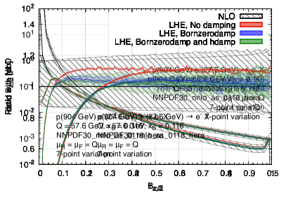
Figure 24: Thrust distribution normalised with respect to $Q$ for $Q=57.6\;\mathrm{GeV}$, $x_{\mathchoice{\displaystyle}{\scriptstyle}{\scriptscriptstyle}{\scriptscriptstyle}\rm B}=0.116$ for the photon-exchange contribution to $e^{-}p\rightarrow e^{-}X$ at NLO (black), and at the LHE level, considering several damping options for the definition of the POWHEG cross section: no damping (red), with the Bornzerodamp mechanism (blue), and with the Bornzerodamp and hdamp mechanisms activated simultaneously (green). In the right panel, the ratio with the NLO curve is shown. The band in the LHE curves is obtained with the 7-point factorisation- and renormalisation-scale variations.

Figure 25: Same as Fig. 24, but for the broadening distribution of Eq. (30).

In Figs. 24 and 25 we compare NLO predictions with distributions obtained from unshowered LHE events, produced using these three definitions of the singular contribution entering the POWHEG cross section ${\rm d}\sigma_{\mathchoice{\displaystyle}{\scriptstyle}{\scriptscriptstyle}{\scriptscriptstyle}\rm PWG}$ of Sec. 2.2.1 for $\tau_{\rm z,Q}$ of Eq. (29) and $B_{\rm z,E}$ of Eq. (30). For small values of the event shapes, all the LHE level distributions agree with each other, and the presence of the POWHEG Sudakov form factor of Eq. (9) regulates the divergent behaviour, which is instead present at NLO.

We observe that if we do not introduce any damping factor, the LHE distribution overshoots the NLO one by roughly 10% in the tail. This enhancement is within the scale-uncertainty band of the NLO result. However, we notice the scale-variation band for the LHE curve is almost absent. This is due to the fact that the hardest radiation is always generated using the transverse momentum as scale entering the emission probability Frixione:2007vw , so that the factorisation and renormalisation scale variation affects only the total weight, but not the differential distribution. While the NLO cross section is smaller than the LO one (i.e. $\bar{B}/B\sim 0.965<1$), the increase of the distribution in the tail, is due to higher-order corrections such as those coming from the treatment of the running coupling Catani:1990rr in the squared bracket of Eq. (7), which can capture the bulk of NLL corrections arising from subsequent unresolved emissions, or due to the scale choice in the PDF. The inclusion of a damping function does instead ensure that such corrections are not applied for large values of the event shapes. In this case the central value of the LHE curve aligns with the NLO one. We also notice that in this case, scale-variation bands are larger, as the argument of the PDFs and the coupling constant appearing in the remnant cross section are varied accordingly. The inclusion of the hdamp mechanism, on top of the Bornzerodamp one, leaves the central value of the curve almost unaffected, but increases the size of the uncertainty band in the tail of the distribution. In all cases, however, the scale-uncertainty band produced by LHE-level distributions is much smaller than the NLO one.

Appendix E Central scale choices

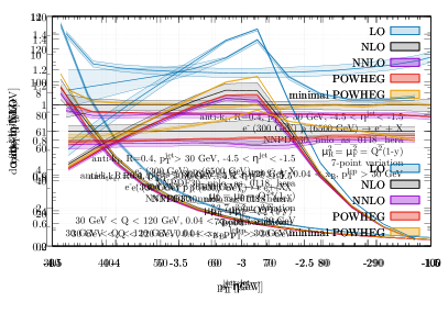
Figure 26: The hardest anti-$k_{T}$ $R=0.4$ jet in the rapidity window $-4.5<\eta^{\mathrm{jet}}<-1.5$ for events satisfying the cuts of Eq. (32). We show LO (blue), NLO (grey), NNLO (purple), our new DIS implementation showered with Pythia8 (red) and the minimally modified POWHEG implementation with the same shower (orange). On the right we show the ratio to the NLO prediction. The bands correspond to a 7-point scale variation around the central scale defined by $\mu^{2}=Q^{2}(1-y)$.

Figure 27: Same as Fig. 26, but now showing the rapidity of the hardest jet satisfying $p_{T}^{\mathrm{jet}}>30\,\mathrm{GeV}$.

In this appendix we present the results of Sec. 3.3 for two different choices for the central value of the renormalisation and factorisation scales. This is of interest since a central scale choice of $\mu^{2}=Q^{2}$ is only well-motivated for inclusive quantities, whereas more exclusive quantities in general probe different QCD scales. The two alternative scales that we explore are the following:

• The transverse momentum of the final-state lepton (in the collision frame), $p_{T}^{\rm\mathchoice{\displaystyle}{\scriptstyle}{\scriptscriptstyle}{\scriptscriptstyle}lep}$, which is related to DIS variables via

  $$\mu^{2}=\left(p_{T}^{\rm\mathchoice{\displaystyle}{\scriptstyle}{\scriptscriptstyle}{\scriptscriptstyle}lep}\right)^{2}=(1-y_{\mathchoice{\displaystyle}{\scriptstyle}{\scriptscriptstyle}{\scriptscriptstyle}\rm DIS})Q^{2}<Q^{2}\,.$$ (148)

  At LO, this scale coincides with the transverse momentum of the jet, $p_{T}^{\rm\mathchoice{\displaystyle}{\scriptstyle}{\scriptscriptstyle}{\scriptscriptstyle}jet}$, and differences between the two scales arise from the real radiation corrections. Such differences are then formally NNLO.

• The invariant mass of the recoil system such that

  $$\mu^{2}=Q^{2}\frac{(1-x_{\mathchoice{\displaystyle}{\scriptstyle}{\scriptscriptstyle}{\scriptscriptstyle}\rm B})}{x_{\mathchoice{\displaystyle}{\scriptstyle}{\scriptscriptstyle}{\scriptscriptstyle}\rm B}}.$$ (149)

  This scale is related to the maximum transverse momentum available for the jet. This choice can be problematic for $x_{\mathchoice{\displaystyle}{\scriptstyle}{\scriptscriptstyle}{\scriptscriptstyle}\rm B}\to 1$, but we want to include it in our discussion to present an extreme scenario.

In the following figures we illustrate the effects of using these two scales both in the fixed order predictions and the POWHEG results.

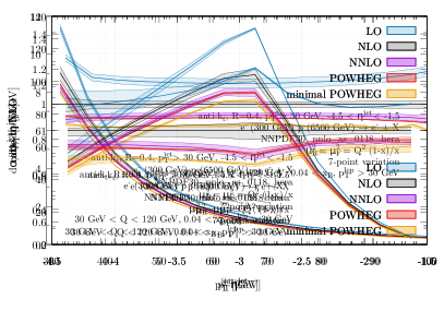
Figure 28: The hardest anti-$k_{T}$ $R=0.4$ jet in the rapidity window $-4.5<\eta^{\mathrm{jet}}<-1.5$ for events satisfying the cuts of Eq. (32). We show LO (blue), NLO (grey), NNLO (purple), our new DIS implementation showered with Pythia8 (red) and the minimally modified POWHEG implementation with the same shower (orange). On the right we show the ratio to the NLO prediction. The bands correspond to a 7-point scale variation around the central scale defined by $\mu^{2}=\frac{Q^{2}(1-x_{\mathchoice{\displaystyle}{\scriptstyle}{\scriptscriptstyle}{\scriptscriptstyle}\rm B})}{x_{\mathchoice{\displaystyle}{\scriptstyle}{\scriptscriptstyle}{\scriptscriptstyle}\rm B}}$.

Figure 29: Same as Fig. 28, but now showing the rapidity of the hardest jet satisfying $p_{T}^{\mathrm{jet}}>30\,\mathrm{GeV}$.

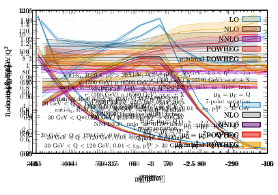
Figure 30: Same as previous figures but now showing the ratio of the POWHEG implementation described in this paper for three different central scale choices. In gray we show $\mu^{2}=Q^{2}$, in red we show $\mu^{2}=Q^{2}(1-y)$, and in yellow we show $\mu^{2}=\frac{Q^{2}(1-x_{\mathchoice{\displaystyle}{\scriptstyle}{\scriptscriptstyle}{\scriptscriptstyle}\rm B})}{x_{\mathchoice{\displaystyle}{\scriptstyle}{\scriptscriptstyle}{\scriptscriptstyle}\rm B}}$. The plot shows the ratio with respect to the $\mu^{2}=Q^{2}$ result.

In Figs. 26–27 we show the results for the first scale, i.e. the transverse momentum of the lepton. As can be seen by comparing to the plots of Figs. 12–13 using $\mu^{2}=Q^{2}$, in Figs. 26–27 the pattern across the various orders is very similar. This is perhaps not a surprise, since for the setup we study here the values of $y_{\mathchoice{\displaystyle}{\scriptstyle}{\scriptscriptstyle}{\scriptscriptstyle}\rm DIS}$ that we probe tend to be small.

For the second scale choice we expect a much larger deviation from $Q$, since for $x_{\mathchoice{\displaystyle}{\scriptstyle}{\scriptscriptstyle}{\scriptscriptstyle}\rm B}>0.04$ this scale can get $24$ times larger than $Q^{2}$ (and also much smaller although only when $x_{\mathchoice{\displaystyle}{\scriptstyle}{\scriptscriptstyle}{\scriptscriptstyle}\rm B}>0.5$). In Figs. 28–29 we show the results for $p_{T}^{\mathrm{jet}}$ and $\eta^{\mathrm{jet}}$ using this scale. Here it can be seen that the size of the perturbative corrections seems to have shifted. In particular the NLO+PS results now sit completely outside of the scale variation band at NLO – this is particularly bad for the minimal POWHEG implementation. Interestingly using the mappings presented in this paper, there seems to still be very good agreement with the NNLO prediction.

Finally, in Fig. 30 we compare all three scale choices, showing their ratio to the scale choice $\mu=Q$. It is interesting to note that despite the rather different pattern observed for the scale defined by $\mu^{2}=\frac{Q^{2}(1-x_{\mathchoice{\displaystyle}{\scriptstyle}{\scriptscriptstyle}{\scriptscriptstyle}\rm B})}{x_{\mathchoice{\displaystyle}{\scriptstyle}{\scriptscriptstyle}{\scriptscriptstyle}\rm B}}$ all three predictions are in reasonably good agreement with each other. The scale uncertainties are a bit underestimated as expected, but not dramatically so.

References

- (1) H1, ZEUS collaboration, F. D. Aaron et al., Combined Measurement and QCD Analysis of the Inclusive e+- p Scattering Cross Sections at HERA, JHEP 01 (2010) 109 [0911.0884].
- (2) H1, ZEUS collaboration, H. Abramowicz et al., Combination and QCD Analysis of Charm Production Cross Section Measurements in Deep-Inelastic ep Scattering at HERA, Eur. Phys. J. C 73 (2013) 2311 [1211.1182].
- (3) H1, ZEUS collaboration, H. Abramowicz et al., Combination of measurements of inclusive deep inelastic scattering cross sections and QCD analysis of HERA data, Eur. Phys. J. C 75 (2015) 580 [1506.06042].
- (4) H1, ZEUS collaboration, H. Abramowicz et al., Combination and QCD analysis of charm and beauty production cross-section measurements in deep inelastic scattering at HERA, Eur. Phys. J. C 78 (2018) 473 [1804.01019].
- (5) H1 collaboration, T. Ahmed et al., Hard scattering in gamma p interactions, Phys. Lett. B 297 (1992) 205.
- (6) ZEUS collaboration, M. Derrick et al., Measurement of total and partial photon proton cross-sections at 180-GeV center-of-mass energy, Z. Phys. C 63 (1994) 391.
- (7) H1 collaboration, C. Adloff et al., Inclusive D0 and D*+- production in deep inelastic e p scattering at HERA, Z. Phys. C 72 (1996) 593 [hep-ex/9607012].
- (8) ZEUS collaboration, J. Breitweg et al., Comparison of ZEUS data with standard model predictions for scattering at high x and , Z. Phys. C 74 (1997) 207 [hep-ex/9702015].
- (9) H1 collaboration, C. Adloff et al., Measurement of open beauty production at HERA, Phys. Lett. B 467 (1999) 156 [hep-ex/9909029].
- (10) H1 collaboration, C. Adloff et al., Deep inelastic inclusive e p scattering at low x and a determination of alpha(s), Eur. Phys. J. C 21 (2001) 33 [hep-ex/0012053].
- (11) ZEUS collaboration, S. Chekanov et al., Inclusive jet cross-sections in the Breit frame in neutral current deep inelastic scattering at HERA and determination of alpha(s), Phys. Lett. B 547 (2002) 164 [hep-ex/0208037].
- (12) ZEUS collaboration, S. Chekanov et al., Measurement of D*+- production in deep inelastic e+- p scattering at HERA, Phys. Rev. D 69 (2004) 012004 [hep-ex/0308068].
- (13) ZEUS collaboration, S. Chekanov et al., An NLO QCD analysis of inclusive cross-section and jet-production data from the zeus experiment, Eur. Phys. J. C 42 (2005) 1 [hep-ph/0503274].
- (14) H1 collaboration, F. D. Aaron et al., Measurement of the Inclusive Scattering Cross Section at Low and at HERA, Eur. Phys. J. C 63 (2009) 625 [0904.0929].
- (15) H1 collaboration, I. Abt et al., A Search for leptoquarks, leptogluons and excited leptons in H1 at HERA, Nucl. Phys. B 396 (1993) 3.
- (16) H1 collaboration, C. Adloff et al., A Search for leptoquark bosons and lepton flavor violation in collisions at HERA, Eur. Phys. J. C 11 (1999) 447 [hep-ex/9907002].
- (17) H1 collaboration, A. Aktas et al., A General search for new phenomena in ep scattering at HERA, Phys. Lett. B 602 (2004) 14 [hep-ex/0408044].
- (18) ZEUS collaboration, M. Derrick et al., Search for leptoquarks with the ZEUS detector, Phys. Lett. B 306 (1993) 173.
- (19) PDF4LHC Working Group collaboration, R. D. Ball et al., The PDF4LHC21 combination of global PDF fits for the LHC Run III, J. Phys. G 49 (2022) 080501 [2203.05506].
- (20) Y. L. Dokshitzer, Calculation of the Structure Functions for Deep Inelastic Scattering and e+ e- Annihilation by Perturbation Theory in Quantum Chromodynamics., Sov. Phys. JETP 46 (1977) 641.
- (21) V. N. Gribov and L. N. Lipatov, Deep inelastic e p scattering in perturbation theory, Sov. J. Nucl. Phys. 15 (1972) 438.
- (22) G. Altarelli and G. Parisi, Asymptotic Freedom in Parton Language, Nucl. Phys. B 126 (1977) 298.
- (23) 2020 Update of the European Strategy for Particle Physics, tech. rep., Geneva, 2020. 10.17181/CERN.JSC6.W89E.
- (24) R. Abdul Khalek et al., Science Requirements and Detector Concepts for the Electron-Ion Collider: EIC Yellow Report, Nucl. Phys. A 1026 (2022) 122447 [2103.05419].
- (25) O. Brüning, A. Seryi and S. Verdú-Andrés, Electron-Hadron Colliders: EIC, LHeC and FCC-eh, Front. in Phys. 10 (2022) 886473.
- (26) R. Abdul Khalek et al., Snowmass 2021 White Paper: Electron Ion Collider for High Energy Physics, in 2022 Snowmass Summer Study, 3, 2022, 2203.13199.
- (27) G. Heinrich, Collider Physics at the Precision Frontier, Phys. Rept. 922 (2021) 1 [2009.00516].
- (28) F. Gross et al., 50 Years of Quantum Chromodynamics, 2212.11107.
- (29) S. Moch, J. A. M. Vermaseren and A. Vogt, The Longitudinal structure function at the third order, Phys. Lett. B 606 (2005) 123 [hep-ph/0411112].
- (30) J. A. M. Vermaseren, A. Vogt and S. Moch, The Third-order QCD corrections to deep-inelastic scattering by photon exchange, Nucl. Phys. B 724 (2005) 3 [hep-ph/0504242].
- (31) S. Moch, J. A. M. Vermaseren and A. Vogt, Third-order QCD corrections to the charged-current structure function F(3), Nucl. Phys. B 813 (2009) 220 [0812.4168].
- (32) J. Davies, A. Vogt, S. Moch and J. A. M. Vermaseren, Non-singlet coefficient functions for charged-current deep-inelastic scattering to the third order in QCD, PoS DIS2016 (2016) 059 [1606.08907].
- (33) J. Blümlein, P. Marquard, C. Schneider and K. Schönwald, The massless three-loop Wilson coefficients for the deep-inelastic structure functions F2, FL, xF3 and g1, JHEP 11 (2022) 156 [2208.14325].
- (34) M. Cacciari, F. A. Dreyer, A. Karlberg, G. P. Salam and G. Zanderighi, Fully Differential Vector-Boson-Fusion Higgs Production at Next-to-Next-to-Leading Order, Phys. Rev. Lett. 115 (2015) 082002 [1506.02660].
- (35) J. Currie, T. Gehrmann, E. W. N. Glover, A. Huss, J. Niehues and A. Vogt, N3LO corrections to jet production in deep inelastic scattering using the Projection-to-Born method, JHEP 05 (2018) 209 [1803.09973].
- (36) T. Gehrmann, A. Huss, J. Niehues, A. Vogt and D. M. Walker, Jet production in charged-current deep-inelastic scattering to third order in QCD, Phys. Lett. B 792 (2019) 182 [1812.06104].
- (37) P. Nason, A New method for combining NLO QCD with shower Monte Carlo algorithms, JHEP 11 (2004) 040 [hep-ph/0409146].
- (38) S. Frixione, P. Nason and C. Oleari, Matching NLO QCD computations with Parton Shower simulations: the POWHEG method, JHEP 11 (2007) 070 [0709.2092].
- (39) S. Frixione and B. R. Webber, Matching NLO QCD computations and parton shower simulations, JHEP 06 (2002) 029 [hep-ph/0204244].
- (40) S. Alioli, P. Nason, C. Oleari and E. Re, A general framework for implementing NLO calculations in shower Monte Carlo programs: the POWHEG BOX, JHEP 06 (2010) 043 [1002.2581].
- (41) J. Alwall, R. Frederix, S. Frixione, V. Hirschi, F. Maltoni, O. Mattelaer et al., The automated computation of tree-level and next-to-leading order differential cross sections, and their matching to parton shower simulations, JHEP 07 (2014) 079 [1405.0301].
- (42) M. Bahr et al., Herwig++ Physics and Manual, Eur. Phys. J. C 58 (2008) 639 [0803.0883].
- (43) J. Bellm et al., Herwig 7.2 release note, Eur. Phys. J. C 80 (2020) 452 [1912.06509].
- (44) T. Gleisberg, S. Hoeche, F. Krauss, M. Schonherr, S. Schumann, F. Siegert et al., Event generation with SHERPA 1.1, JHEP 02 (2009) 007 [0811.4622].
- (45) Sherpa collaboration, E. Bothmann et al., Event Generation with Sherpa 2.2, SciPost Phys. 7 (2019) 034 [1905.09127].
- (46) T. Sjöstrand, S. Ask, J. R. Christiansen, R. Corke, N. Desai, P. Ilten et al., An introduction to PYTHIA 8.2, Comput. Phys. Commun. 191 (2015) 159 [1410.3012].
- (47) C. Bierlich et al., A comprehensive guide to the physics and usage of PYTHIA 8.3, 2203.11601.
- (48) G. A. Schuler and H. Spiesberger, DJANGO: The Interface for the event generators HERACLES and LEPTO, in Workshop on Physics at HERA, 1991.
- (49) S. Catani and M. H. Seymour, A General algorithm for calculating jet cross-sections in NLO QCD, Nucl. Phys. B 485 (1997) 291 [hep-ph/9605323].
- (50) D. Graudenz, Disaster++: Version 1.0, hep-ph/9710244.
- (51) Z. Nagy and Z. Trocsanyi, Multijet cross-sections in deep inelastic scattering at next-to-leading order, Phys. Rev. Lett. 87 (2001) 082001 [hep-ph/0104315].
- (52) M. Dasgupta and G. P. Salam, Resummed event shape variables in DIS, JHEP 08 (2002) 032 [hep-ph/0208073].
- (53) A. Banfi, G. P. Salam and G. Zanderighi, Principles of general final-state resummation and automated implementation, JHEP 03 (2005) 073 [hep-ph/0407286].
- (54) M. Knobbe, D. Reichelt and S. Schumann, (N)NLO+NLL’ accurate predictions for plain and groomed 1-jettiness in neutral current DIS, 2306.17736.
- (55) T. Carli, T. Gehrmann and S. Hoeche, Hadronic final states in deep-inelastic scattering with Sherpa, Eur. Phys. J. C 67 (2010) 73 [0912.3715].
- (56) S. Höche, S. Kuttimalai and Y. Li, Hadronic Final States in DIS at NNLO QCD with Parton Showers, Phys. Rev. D 98 (2018) 114013 [1809.04192].
- (57) https://powhegbox.mib.infn.it.
- (58) L. Buonocore, P. Nason, F. Tramontano and G. Zanderighi, Photon and leptons induced processes at the LHC, JHEP 12 (2021) 073 [2109.10924].
- (59) L. Buonocore, A. Greljo, P. Krack, P. Nason, N. Selimovic, F. Tramontano et al., Resonant leptoquark at NLO with POWHEG, JHEP 11 (2022) 129 [2209.02599].
- (60) T. Ježo and P. Nason, On the Treatment of Resonances in Next-to-Leading Order Calculations Matched to a Parton Shower, JHEP 12 (2015) 065 [1509.09071].
- (61) S. Ferrario Ravasio, P. Nason and C. Oleari, All-orders behaviour and renormalons in top-mass observables, JHEP 01 (2019) 203 [1810.10931].
- (62) S. Frixione, Z. Kunszt and A. Signer, Three jet cross-sections to next-to-leading order, Nucl. Phys. B 467 (1996) 399 [hep-ph/9512328].
- (63) S. Catani, B. R. Webber and G. Marchesini, QCD coherent branching and semiinclusive processes at large x, Nucl. Phys. B 349 (1991) 635.
- (64) P. Nason and B. Webber, Next-to-Leading-Order Event Generators, Ann. Rev. Nucl. Part. Sci. 62 (2012) 187 [1202.1251].
- (65) Particle Data Group collaboration, R. L. Workman et al., Review of Particle Physics, PTEP 2022 (2022) 083C01.
- (66) H1 collaboration, F. D. Aaron et al., Inclusive Deep Inelastic Scattering at High with Longitudinally Polarised Lepton Beams at HERA, JHEP 09 (2012) 061 [1206.7007].
- (67) NNPDF collaboration, R. D. Ball et al., Parton distributions for the LHC Run II, JHEP 04 (2015) 040 [1410.8849].
- (68) A. Buckley, J. Ferrando, S. Lloyd, K. Nordström, B. Page, M. Rüfenacht et al., LHAPDF6: parton density access in the LHC precision era, Eur. Phys. J. C 75 (2015) 132 [1412.7420].
- (69) A. Karlberg, “disorder: Deep inelastic scattering at high orders.” CERN-TH-2023-XXX, 2023.
- (70) G. P. Salam and J. Rojo, A Higher Order Perturbative Parton Evolution Toolkit (HOPPET), Comput. Phys. Commun. 180 (2009) 120 [0804.3755].
- (71) F. A. Dreyer and A. Karlberg, Vector-Boson Fusion Higgs Production at Three Loops in QCD, Phys. Rev. Lett. 117 (2016) 072001 [1606.00840].
- (72) F. A. Dreyer and A. Karlberg, Vector-Boson Fusion Higgs Pair Production at N3LO, Phys. Rev. D 98 (2018) 114016 [1811.07906].
- (73) F. A. Dreyer and A. Karlberg, Fully differential Vector-Boson Fusion Higgs Pair Production at Next-to-Next-to-Leading Order, Phys. Rev. D 99 (2019) 074028 [1811.07918].
- (74) W. L. van Neerven and A. Vogt, NNLO evolution of deep inelastic structure functions: The Nonsinglet case, Nucl. Phys. B 568 (2000) 263 [hep-ph/9907472].
- (75) W. L. van Neerven and A. Vogt, NNLO evolution of deep inelastic structure functions: The Singlet case, Nucl. Phys. B 588 (2000) 345 [hep-ph/0006154].
- (76) B. Cabouat and T. Sjöstrand, Some Dipole Shower Studies, Eur. Phys. J. C 78 (2018) 226 [1710.00391].
- (77) S. Alioli et al., Update of the Binoth Les Houches Accord for a standard interface between Monte Carlo tools and one-loop programs, Comput. Phys. Commun. 185 (2014) 560 [1308.3462].
- (78) P. Nason and C. Oleari, NLO Higgs boson production via vector-boson fusion matched with shower in POWHEG, JHEP 02 (2010) 037 [0911.5299].
- (79) B. Jager, S. Schneider and G. Zanderighi, Next-to-leading order QCD corrections to electroweak Zjj production in the POWHEG BOX, JHEP 09 (2012) 083 [1207.2626].
- (80) S. Alioli, P. Nason, C. Oleari and E. Re, NLO single-top production matched with shower in POWHEG: s- and t-channel contributions, JHEP 09 (2009) 111 [0907.4076].
- (81) R. Frederix, E. Re and P. Torrielli, Single-top t-channel hadroproduction in the four-flavour scheme with POWHEG and aMC@NLO, JHEP 09 (2012) 130 [1207.5391].
- (82) R. Devenish and A. Cooper-Sarkar, Deep inelastic scattering. 2004, 10.1093/acprof:oso/9780198506713.001.0001.
- (83) A. Banfi, G. P. Salam and G. Zanderighi, Phenomenology of event shapes at hadron colliders, JHEP 06 (2010) 038 [1001.4082].
- (84) H1 collaboration, A. Aktas et al., Measurement of event shape variables in deep-inelastic scattering at HERA, Eur. Phys. J. C 46 (2006) 343 [hep-ex/0512014].
- (85) V. Antonelli, M. Dasgupta and G. P. Salam, The Resummed thrust distribution in DIS, J. Phys. G 26 (2000) 658 [hep-ph/9910343].
- (86) I. Borsa, D. de Florian and I. Pedron, Jet Production in Polarized Deep Inelastic Scattering at Next-to-Next-to-Leading Order, Phys. Rev. Lett. 125 (2020) 082001 [2005.10705].
- (87) I. Borsa, D. de Florian and I. Pedron, Inclusive-jet and dijet production in polarized deep inelastic scattering, Phys. Rev. D 103 (2021) 014008 [2010.07354].
- (88) M. Cacciari, G. P. Salam and G. Soyez, The anti- jet clustering algorithm, JHEP 04 (2008) 063 [0802.1189].
- (89) M. Cacciari, G. P. Salam and G. Soyez, FastJet User Manual, Eur. Phys. J. C 72 (2012) 1896 [1111.6097].
- (90) H. Brooks, C. T. Preuss and P. Skands, Sector Showers for Hadron Collisions, JHEP 07 (2020) 032 [2003.00702].
- (91) S. Höche, S. Mrenna, S. Payne, C. T. Preuss and P. Skands, A Study of QCD Radiation in VBF Higgs Production with Vincia and Pythia, SciPost Phys. 12 (2022) 010 [2106.10987].
- (92) S. Ferrario Ravasio and C. Oleari, NLO + parton-shower generator for Wc production in the POWHEG BOX RES, 2304.13791.
- (93) M. Dasgupta and G. P. Salam, Event shapes in e+ e- annihilation and deep inelastic scattering, J. Phys. G 30 (2004) R143 [hep-ph/0312283].
- (94) I. Borsa, D. de Florian and I. Pedron, NNLO jet production in neutral and charged current polarized deep inelastic scattering, Phys. Rev. D 107 (2023) 054027 [2212.06625].
- (95) J. Butterworth et al., PDF4LHC recommendations for LHC Run II, J. Phys. G 43 (2016) 023001 [1510.03865].
- (96) M. van Beekveld and S. Ferrario Ravasio, Next-to-leading-logarithmic PanScales showers for Deep Inelastic Scattering and Vector Boson Fusion, JHEP 02 (2024) 001 [2207.09467].
- (97) M. van Beekveld, S. Ferrario Ravasio, K. Hamilton, G. P. Salam, A. Soto-Ontoso, G. Soyez et al., PanScales showers for hadron collisions: all-order validation, JHEP 11 (2022) 020 [2207.09467].
- (98) K. Hamilton, A. Karlberg, G. P. Salam, L. Scyboz and R. Verheyen, Matching and event-shape NNDL accuracy in parton showers, JHEP 03 (2023) 224 [2301.09645].