Exploiting Spatial-temporal Data for Sleep Stage Classification via Hypergraph Learning

Abstract

Sleep stage classification is crucial for detecting patients’ health conditions. Existing models, which mainly use Convolutional Neural Networks (CNN) for modelling Euclidean data and Graph Convolution Networks (GNN) for modelling non-Euclidean data, are unable to consider the heterogeneity and interactivity of multimodal data as well as the spatial-temporal correlation simultaneously, which hinders a further improvement of classification performance. In this paper, we propose a dynamic learning framework STHL, which introduces hypergraph to encode spatial-temporal data for sleep stage classification. Hypergraphs can construct multi-modal/multi-type data instead of using simple pairwise between two subjects. STHL creates spatial and temporal hyperedges separately to build node correlations, then it conducts type-specific hypergraph learning process to encode the attributes into the embedding space. Extensive experiments show that our proposed STHL outperforms the state-of-the-art models in sleep stage classification tasks.

Index Terms—  Sleep stage classification, multimodal physiological signal, hypergraph learning

1 Introduction

Scientific sleep stage classification is of significance to the diagnosis of sleep disorders to enhance the sleep quality. As a key reference, polysomnography (PSG) is utilised to classify the sleep stages. PSG records the physical signals of different organs of the human body. These signals include electroencephalography (EEG), electrooculography (EOG), electromyography (EMG), and electrocardiography (ECG). The interactions between organs and the influences of adjacent timestamps render the observations non-independent. Therefore, the data recorded by PSG is considered spatial-temporal [1, 2], which is associated with time series and spatial geographic location. Meanwhile, substantial differences exist in the spectrograms recorded from multiple organs in PSG, and thus it is also crucial to utilise the multimodal signals originated from different signal source types, e.g., EOG signals and ECG signals. Besides the spatial-temporal correlations of the data, two properties also need to be considered when handling these multimodal signals for sleep stage classification: the interactivity that indicates the continuous interaction of human organs during sleep periods [3], and the heterogeneity that represents the difference in spectrograms exhibited when detecting different signals  [4].

Recently, deep learning based methods [5], such as Convolutional Neural Networks (CNN) and Recurrent Neural Network (RNN), have been widely studied to solve the sleep stage classification problem due to their powerful representation learning capabilities. However, the process of CNN/RNN requires the image data to be represented as a regular grid-like (Euclidean) data structure, i.e., a grid of pixels. Apart from that, it is pointed out that prior models fail to capture the implicit correlations in the data simultaneously [6]. To alleviate this limitation, Graph Neural Network (GNN), which is a neural network designed for handling graph data, has garnered significant attention in addressing the generation of data from non-Euclidean domains [7]. Moreover, hypergraph-based methods start to emerge to process multimodal data efficiently [8]. Compared with the traditional graph learning-based method where each edge connects only two nodes, hypergraphs introduce multiple hyperedges that can connect more than two nodes simultaneously. Therefore, hypergraph is expected to extract high-order correlations from multimodal signals, leading to a superior classification performance.

In this paper, we propose a dynamic learning framework, namely STHL, to achieve accurate sleep stage classification. To the best of our knowledge, this is the first time that hypergraph is utilised to analyse the multimodal signals for sleep stage classification. Our main contributions are summarised as follows: (1) We propose a hypergraph-based framework for sleep stage classification. It includes dynamic hyperedge construction and embedding update and multi-head attentive node embedding update. (2) We design a dynamic learning process to generate spatial and temporal hyperedges separately, forming the hypergraph with better modelling capability. The node embedding is then updated through multi-head attention mechanism to encode the interactivity and heterogeneity into the embedding spaces. (3) We conduct extensive experiments using the real-world dataset, demonstrating that our proposal can outperform comparative methods in sleep stage classification.

2 Related work

2.1 Traditional Learning Methods

Traditional machine learning-based sleep stage classification, such as Support Vector Machine (SVM) [9], Random Forest (RF) [10], and Hidden Markov Model (HMM) [11] not only rely heavily on the quality of feature extraction but also fail to extract important spatial-temporal relationships. On the other hand, while CNN [12] and RNN [5], which are proven effective when extracting the features to improve the classification, these methods rely on grid data input, and thus lack the ability to capture the connections between different brain regions and organs. As a result, incorporating graphs as representative data structures for connections in non-Euclidean spaces is then investigated for accurate modelling.

2.2 Graph-based Learning Methods

Jia et al. [13] proposed GraphSleepNet that introduces a spatial-temporal graph convolutional network to learn the intrinsic connection between different EEG signals adaptively. Developed from GraphSleepNet, two brain views are constructed based on the functional connectivity and physical distance proximity of brain regions, by which a multi-view spatial-temporal map convolutional network (MSTGCN) [14] is constituted. Moreover, SleepHGNN [6] combines the characteristics of heterogeneity and interactivity, while considering the interactions between human organs. However, dynamic spatial-temporal correlation of the data is not included in SleepHGNN.

In light of using attention mechanisms to capture the information between sleep stages [15, 16]. As aforementioned, hypergraphs combine multiple hyperedges with different types for representing higher-order interrelations, and thus it is effective in solving the association problem of multimodal data. In this paper, we introduce the hypergraph-based framework for sleep stage classification, and the hypergraph is constructed dynamically so that implicit spatial-temporal correlations of the data can be encoded.

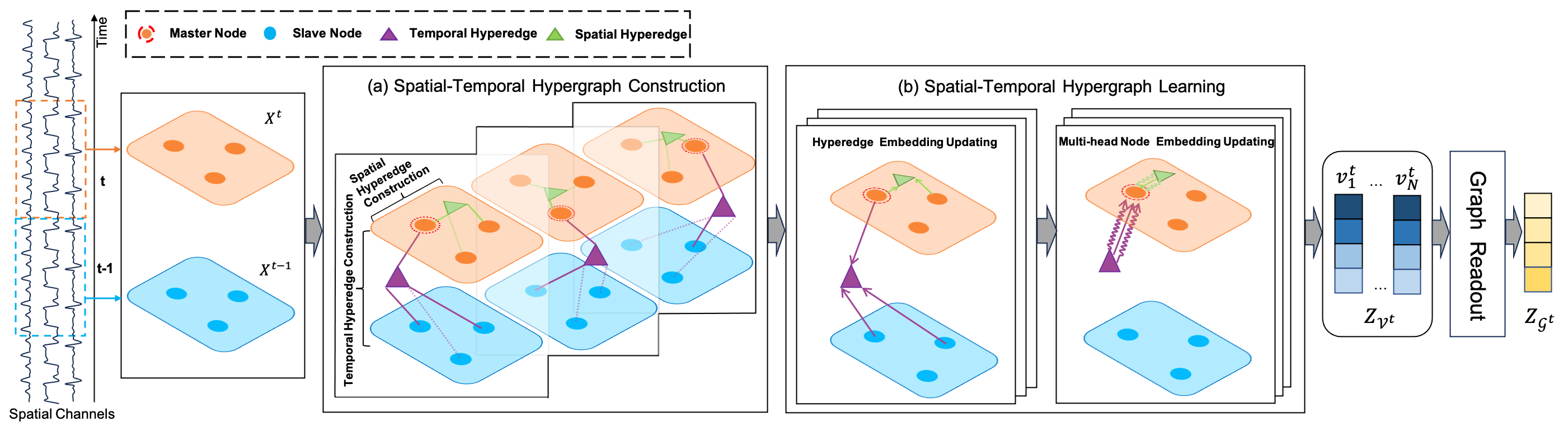
Fig. 1: An overview of STHL

3 methodology

Let $\mathcal{X}\!=\!\left\{\emph{X}^{1},...,\emph{X}^{T}\right\}\in\mathcal{R}^{T\times N\times d}$ denotes a spatial-temporal data containing $T$ timestamps, where $\emph{X}^{t}\!=\!\left\{\emph{x}^{t}_{1},...,\emph{x}^{t}_{N}\right\}\in\mathcal{R}^{N\times d}$ represents the signal of $N$ channels at a timestamp $t$, and the size of each channel feature is $d$ (As shown in the leftmost part of Fig. 1). We define a hypergraph as $\mathcal{G}=\left\{\mathcal{V},\mathcal{E}\right\}$, where $\mathcal{V}$ is the set of node set and E is the set of hyperedges. Each hyperedge $e\in\mathcal{E}$ contains two or more nodes. Since there is no node concept in the spatial-temporal data $\mathcal{X}$, we thus treat each spatial channel as a node at any timestamp $t$. The node set at timestamp $t$ is defined as $\emph{V}^{t}=\left\{v^{t}_{1},...,v^{t}_{N}\right\}$, and the number of nodes in each timestamp is $N$. We use $\emph{Y}=\left\{\emph{y}^{1},...,\emph{y}^{T}\right\}$ to denote the label of each timestamp.

3.1 Spatial-Temporal Hypergraph Construction

The spatial-temporal hypergraph at timestamp $t$ is defined as $\mathcal{G}^{t}=\left\{\mathcal{V}^{t},\mathcal{E}^{t}\right\}$. To model the temporal dependencies among nodes along the time dimension, we utilise the nodes feature of one timestamp previous to capture the historical information [17]. Thus, the node set $\mathcal{V}^{t}$ contains nodes from two consecutive timestamps at $t$, which is defined as $\mathcal{V}^{t}=\left\{\emph{V}^{t},\emph{V}^{t-1}\right\}$. The node feature matrices for these timestamps are $\emph{X}^{t}$ and $\emph{X}^{t-1}$ respectively.

A hyperedege encloses a specific set of nodes with common attributes or implicit data relations, which represents local group information among the nodes. To facilitate hyperedge generation, we introduce two kinds of nodes: master node and slave node. A master node $\dot{v}\in\mathcal{V}$ acts as an anchor when generating the hyperedge $e\left(\dot{v}\right)\in\mathcal{E}$, which is combined with a set of slave nodes $S\left(\dot{v}\right)=\left\{\hat{v}\right\}$ to collectively constitute the hyperedge. We propose a dynamic learning process that generates two types of hyperedges: spatial hyperedges that capture heterogeneity, encoding relations among different channels in one timestamp; temporal hyperedges that scrutinize interactivity, modelling the continuous interaction of channels in consecutive timestamps.

For each master node $\dot{v}^{t}_{i}\in\emph{V}^{t}$ in spatial-temporal hypergraph $\mathcal{G}^{t}$ at timestamp $t$, the spatial hyperedge $e_{spa}\left(\dot{v}_{i}^{t}\right)\in\mathcal{E}^{t}$ can be generated based on the reconstruction of the master node $\dot{v}^{t}_{i}$ and the spatial candidate slave node set $\tilde{S}^{spa}\left(\dot{v}^{t}_{i}\right)=\left\{v|v\in\emph{V}^{t},v\neq\dot{v}^{t}_{i}\right\}$, which is denoted as:

$$c_{spa}\left(\dot{v}^{t}_{i}\right)=\|\emph{X}^{t}\left(\dot{v}^{t}_{i}\right)\cdot\theta_{spa}-\emph{p}^{spa}_{\dot{v}^{t}_{i}}\cdot\emph{X}^{t}\left(\tilde{S}^{spa}\left(\dot{v}^{t}_{i}\right)\right)\|_{2}~{}$$ (1)

where $\left\|\cdot\right\|_{2}$ denotes the $l2$ norm of the vector. $\emph{X}^{t}\left(\dot{v}^{t}_{i}\right)$ and $\emph{X}^{t}\left(\tilde{S}^{spa}\left(\dot{v}^{t}_{i}\right)\right)$ are node feature matrices of the master node and the spatial candidate slave node set respectively. $\theta_{spa}$ is a specific trainable projection matrix when generating the spatial hyperedge $e_{spa}\left(\dot{v}_{i}^{t}\right)\in\mathcal{E}^{t}$. $\emph{p}^{spa}_{\dot{v}^{t}_{i}}\in\mathcal{R}^{\left(N-1\right)}$ denotes the trainable reconstruction coefficient vector for a specific spatial hyperedge, with each element $\emph{p}^{spa}_{\dot{v}^{t}_{i}}\left(v\right)$ representing the learned reconstruction coefficient of the node $v\in\tilde{S}^{spa}\left(\dot{v}^{t}_{i}\right)$. According to $\emph{p}^{spa}_{\dot{v}^{t}_{i}}$, the nodes in the spatial candidate slave node set $\tilde{S}^{spa}\left(\dot{v}^{t}_{i}\right)$ with reconstruction coefficient larger than zero are selected to generate a spatial hyperedge of the master node $\dot{v}^{t}_{i}$, which is denoted as $S^{spa}\left(\dot{v}^{t}_{i}\right)=\left\{v|v\in\tilde{S}^{spa}\left(\dot{v}^{t}_{i}\right),\emph{p}^{spa}_{\dot{v}^{t}_{i}}\left(v\right)>0\right\}$ (connected through green solid lines in Fig. 1). By contrast, unselected nodes with a reconstruction coefficient value below 0 are connected by dotted lines. The spatial reconstruction error $c_{spa}$ measures the deviation of the reconstruction of the master node.

Similarly, as shown in the Fig. 1(a), temporal salve nodes are encircled from $\emph{V}^{t-1}$ to form the temporal hyperedge $e_{tem}\left(\dot{v}_{i}^{t}\right)$ with the master node based on the trainable reconstruction coefficient vector $\emph{p}^{tem}_{\dot{v}^{t}_{i}}$. Overall, the loss of hyperedges generation in one timestamp is defined as:

$$\begin{split}\mathcal{L}_{recon}\!\!=\!\!\!\!\sum_{i=\left[1,...,N\right]}&\!\!\!\!\!\!\lambda\left(c_{spa}\!\left(\dot{v}^{t}_{i}\right)\!+\!c_{tem}\!\left(\dot{v}^{t}_{i}\right)\right)\!+\!\left(\|\emph{p}^{spa}_{\dot{v}^{t}_{i}}\|_{1}+\|\emph{p}^{tem}_{\dot{v}^{t}_{i}}\|_{1}\right)\\ &+\gamma\left(\|\emph{p}^{spa}_{\dot{v}^{t}_{i}}\|_{2}+\|\emph{p}^{tem}_{\dot{v}^{t}_{i}}\|_{2}\right)~{}\end{split}$$ (2)

where $\left\|\cdot\right\|_{1}$ denotes the $l1$ norm of the vector and $c_{tem}$ denotes the reconstruction error of temporal hyperedges. $\lambda$ is the weight hyperparameter of the reconstruction error. $\gamma$ is the regularizing factor to balance $l1$ norm and $l2$ norm of the two types of reconstruction coefficient vectors.

3.2 Spatial-Temporal Hypergraph Learning

3.2.1 Hyperedge Embedding Updating

Let H represents incidence relations between hyperedges and nodes, with entries are $\emph{H}\left(v,e\left(\dot{v}^{t}_{i}\right)\right)=\left\{\small\begin{matrix}1\text{,}&v=\dot{v}^{t}_{i}\\ \emph{p}_{\dot{v}^{t}_{i}}\!\left(\!v\!\right)\!\text{,}&v\in S^{spa}\!\left(\!\dot{v}^{t}_{i}\!\right)\\ 0\text{,}&\text{otherwise}\end{matrix}\right.$. The embedding of hyperedges is aggregated by node features as follows:

$$\emph{E}\left(e\left(\dot{v}^{t}_{i}\right)\right)=\frac{\sum_{v\in\mathcal{V}^{t}}\emph{H}\left(v,e\left(\dot{v}^{t}_{i}\right)\right)\times\emph{X}\left(v\right)}{\sum_{v\in\mathcal{V}^{t}}\emph{H}\left(v,e\left(\dot{v}^{t}_{i}\right)\right)}$$ (3)

3.2.2 Multi-head Node Embedding Updating

We use the spatial hyperedge and the temporal hyperedge associated with the master node $\dot{v}^{t}_{i}$ to update the node embedding. The hyperedges associated with node $\dot{v}^{t}_{i}$ is denoted as $\left\{e_{spa}\left(\dot{v}^{t}_{i}\right),e_{tem}\left(\dot{v}^{t}_{i}\right)\right\}$. We calculate the multi-head attention between a master node and two types of hyperedge, and then use the normalized attention as the weight of the hyperedge. The process of weight calculation for two types of hyperedge is similar, and we thus take calculating spatial hyperedge attention as an example:

$$\begin{split}&\emph{Q}^{h}\left(\dot{v}^{t}_{i}\right)=\emph{X}^{t}\left(\dot{v}^{t}_{i}\right)\cdot Q\text{-}Lin^{h}\\ &\emph{K}_{spa}^{h}\left(\dot{v}^{t}_{i}\right)=\emph{E}\left(e_{spa}\left(\dot{v}^{t}_{i}\right)\right)\cdot K\text{-}Lin^{h}_{spa}\\ &att^{h}\left(\dot{v}^{t}_{i},e_{spa}\left(\dot{v}^{t}_{i}\right)\right)=\frac{\emph{Q}^{h}\left(\dot{v}^{t}_{i}\right)\cdot\Theta_{spa}^{att}\cdot\emph{K}_{spa}^{h}\left(\dot{v}^{t}_{i}\right)^{T}}{\sqrt{d}}\end{split}$$ (4)

First, for the $h$-th attention head $att^{h}\left(\dot{v}^{t}_{i},e_{spa}\left(\dot{v}^{t}_{i}\right)\right)$, we project the master node into the $h$-th query vector $\emph{Q}^{h}\left(\dot{v}^{t}_{i}\right)$ with a linear transformation matrix $Q\text{-}Lin^{h}\in\mathcal{R}^{d\times\frac{d}{K}}$, where $K$ is the number of attention heads. We also project the spatial hyperedge $e_{spa}\left(\dot{v}^{t}_{i}\right)$ into the $h$-th key vector $\emph{K}_{spa}^{h}\left(\dot{v}^{t}_{i}\right)$ on the same dimension. Next, we apply a trainable weight matrix $\Theta_{spa}^{att}\in\mathcal{R}^{\frac{d}{K}\times\frac{d}{K}}$ to obtain $h$-th spatial attention, and $\sqrt{d}$ acts a scaling factor. The $h$-th temporal attention $att^{h}\left(\dot{v}^{t}_{i},e_{tem}\left(\dot{v}^{t}_{i}\right)\right)$ is calculated in a similar manner. Finally, the weight of the spatial hyperedge $w^{h}_{spa}\left(\dot{v}^{t}_{i}\right)$ and the temporal hyperedge $w^{h}_{tem}\left(\dot{v}^{t}_{i}\right)$ are calculated by $softmax$ normalization. The attentive aggregation of different heads among hyperedges for updating node embedding of $\dot{v}_{i}^{t}$ (reffered to as wavy lines in Fig  1(b)) is denoted as :

$$\begin{split}\emph{Z}_{\emph{V}^{t}}\left(\dot{v}^{t}_{i}\right)=MLP(\mathop{\operatorname*{\mathchoice{\Big{\|}}{\big{\|}}{\|}{\|}}}\limits_{h\in\left[1,K\right]}&(w^{h}_{spa}\left(\dot{v}^{t}_{i}\right)\times\emph{K}_{spa}^{h}\left(\dot{v}^{t}_{i}\right)\\ &+w^{h}_{tem}\left(\dot{v}^{t}_{i}\right)\times\emph{K}_{tem}^{h}\left(\dot{v}^{t}_{i}\right)))\end{split}~{}$$ (5)

where $\operatorname*{\mathchoice{\Big{\|}}{\big{\|}}{\|}{\|}}$ represents concatenation. We first aggregate two types of hyperedges associated with the master node, and then concatenate all $K$ heads. After that, the node embedding of $\dot{v}^{t}_{i}$ is updated by a shallow multi-layer perceptron (MLP). We average the node embedding of all nodes $\emph{Z}_{\emph{V}^{t}}$ at timestamp $t$ to read-out the graph representation of $\mathcal{G}^{t}$, which is denoted as $\emph{Z}_{\mathcal{G}^{t}}\in\mathcal{R}^{d}$.

To realise STHL in an end-to-end fashion, the loss function used in the training process is denoted as:

$$\mathcal{L}=\alpha\mathcal{L}_{recon}+\left(1-\alpha\right)CE\left(MLP\left(\emph{Z}_{\mathcal{G}^{t}}\right),\emph{y}^{t}\right)$$ (6)

The $MLP$ is used to map from graph representation to label space, and the cross-entropy function (CE) measures the difference between predicted labels and true labels of graphs. $\alpha$ is a weight hyperparameter to trade off the effects of reconstruction loss and the loss of graph classification.

4 experiments

4.1 Experimental Setting

The evaluation of STHL is performed based on the ISRUC Subgroup-3 dataset [18], which encompasses PSG recordings collected from 10 healthy subjects. The time-series data is extracted by decomposing each PSG recording into 6 EEG channels, 2 EOG channels, 1 EMG channel and 1 ECG channel. To make a fair comparison with other state-of-the-art baselines, all 10 channels are employed as the input into our model. While the raw signal contains a feature dimension of 6000, we use a Covolutational Neural Network  [13] for feature extraction, reducing the dimension down to 256.

The proposed model is compared with five baseline methods that fall into traditional and graph-based categories. Support Vector Machine (SVM) [9] is a traditional machine learning method that learns the classification boundary by optimizing the hinge loss. Random Forest (RF) [10] introduces the bagging strategy to perform classification, with the help of multiple decision trees. DeepSleepNet [19] is a deep learning based method that encodes spatial signal information using convolution neural network and temporal signal information with the Bi-LSTM network. Multi-View Spatial-Temporal Graph Convolution Network (MSTGCN) [14] is a graph learning based method that employs the attention mechanism and spatial-temporal network to capture the signal information. SleepHGNN [6] is a graph learning based method that constructs a heterogeneous graph based on the mutual information between channels, Heterogeneous Graph Transformer is further applied to perform graph-level classification. We follow the data pre-processing steps and the default model structures reported in the original papers for all the baselines introduced above. For SVM, RF, DeepSleepNet and STHL, we provide spatial-temporal data from two consecutive timestamps $\left\{\emph{X}^{t-1},\emph{X}^{t}\right\}$, while the data for MSTGCN is provided within a temporal window with size of 5, i.e., $\left\{\emph{X}^{t-2},\emph{X}^{t-1},\emph{X}^{t},\emph{X}^{t+1},\emph{X}^{t+2}\right\}$, in accordance with its reported experimental setting. Feature extraction network is applied for dimensional reduction for both MSTGCN and STHL. Regarding the hyperparameters in the reconstruction loss function, $\lambda$ is set to 0.01, $\gamma$ to 0.2 and $\alpha$ to 0.1, respectively.

4.2 Experimental Results

The experimental results are summarised in Table 1, with weighted F1-score and Accuracy applied as the evaluation metrics. On average, STHL outperforms the traditional models with 15.4% average performance gain in F1 score and 12.1% in Accuracy, respectively. It indicates that the traditional models are incapable of simultaneously capturing spatial information and temporal information due to the simpleness of model structures, while STHL updates node embeddings based on both spatial and temporal hyperedges, resulting in better modelling capability for spatial-temporal data. Compared with graph-based models, STHL achieves an average performance gain of 2.9% in F1 score and 3.7% in Accuracy. MSTGCN and SleepHGNN can only perform pairwise message passing between adjacent nodes, whereas STHL uncovers the implicit information through the constructed hyperedges.

Models		F1	Accuracy
Traditional Model	SVM	0.653	0.720
	RF	0.612	0.699
	DeepSleepNet	0.766	0.767
Graph Based Model	MSTGCN	0.824	0.829
	SleepHGNN	0.779	0.795
	STHL	0.831	0.849

Table 1: Evaluation Result

Model Setting	F1	Accuracy
Default	0.849	0.831
w/o Hyperedge	0.782	0.774
w/o Attention	0.818	0.806

Table 2: Ablation Study Result

The performance gain of STHL is mainly contributed by the hyperedge reconstruction and the multi-head attentive node embedding updating. Two model variants are delineated in Table 2 for further analysis. We first study the effect without using the hyperedges, in which the vanilla graph convolution layer is utilised to update nodes with spatial information. Note the adjacency matrix is calculated using Pearson coefficients between node embeddings to quantify the connectivity. Nodes are updated with temporal information based on the weighted sum of node embeddings from previous and current timestamps. Removing hyperedges results in a 6.7% performance drop in F1 score and a 5.7% drop in Accuracy due to the elimination of learnable reconstruction parameters. The second variant of the model relates to removing the multi-head attentive layer when updating node embeddings. The variant results in a 3.1% drop in F1 score and a 2.5% drop in Accuracy, inferring the necessity of modelling spatial and temporal hyperedges separately with attention weights.

5 conclusion

We propose a novel hypergraph model for sleep stage classification, which contains dynamic hyperedges generation and spatial-temporal hypergraph learning. The node embedding is updated through type-specific attention, aiming to encode the heterogeneity and interactivity into the embedding space. Experimental results demonstrate that STHL outperforms the state-of-the-art models on the sleep stage classification.

References

- [1] Shengnan Guo, Youfang Lin, Ning Feng, Chao Song, and Huaiyu Wan, “Attention based spatial-temporal graph convolutional networks for traffic flow forecasting,” in AAAI, 2019, pp. 922–929.
- [2] Bing Yu, Haoteng Yin, and Zhanxing Zhu, “Spatio-temporal graph convolutional networks: A deep learning framework for traffic forecasting,” in IJCAI, 2018, pp. 3634–3640.
- [3] Plamen Ch. Ivanov, Jilin W. J. L. Wang, and Xiyun Zhang, “Signal processing in network physiology: quantifying network dynamics of organ interactions,” in EUSIPCO, 2021, pp. 945–949.
- [4] Xilin Li, Ahmed Al-Ani, and Sai Ho Ling, “Feature selection for the detection of sleep apnea using multi-bio signals from overnight polysomnography,” in EMBC, 2018, pp. 1444–1447.
- [5] Luigi Fiorillo et al., “Automated sleep scoring: A review of the latest approaches,” Sleep Medicine Reviews, vol. 48, pp. 1–12, 2019.
- [6] Ziyu Jia et al., “Exploiting interactivity and heterogeneity for sleep stage classification via heterogeneous graph neural network,” in ICASSP, 2023, pp. 1–5.
- [7] David Ahmedt-Aristizabal, Mohammad Ali Armin, Simon Denman, Clinton Fookes, and Lars Petersson, “Graph-based deep learning for medical diagnosis and analysis: Past, present and future,” Sensors, vol. 21, no. 14, pp. 1–41, 2021.
- [8] Yue Gao, Yifan Feng, Shuyi Ji, and Rongrong Ji, “HGNN+: General hypergraph neural networks,” IEEE Transactions on Pattern Analysis and Machine Intelligence, vol. 45, no. 3, pp. 3181–3199, 2023.
- [9] Ahnaf Rashik Hassan and Mohammed Imamul Hassan Bhuiyan, “A decision support system for automatic sleep staging from EEG signals using tunable q-factor wavelet transform and spectral features,” Journal of Neuroscience Methods, vol. 271, pp. 107–118, 2016.
- [10] Wu Huang et al., “Sleep staging algorithm based on multichannel data adding and multifeature screening,” Computer Methods and Programs in Biomedicine, vol. 187, pp. 1–15, 2020.
- [11] Shing-Tai Pan, Chih-En Kuo, Jian-Hong Zeng, and Sheng-Fu Liang, “A transition-constrained discrete hidden markov model for automatic sleep staging,” BioMedical Engineering OnLine, vol. 11, no. 1, pp. 1–19, 2012.
- [12] Stanislas Chambon, Mathieu N. Galtier, Pierrick J. Arnal, Gilles Wainrib, and Alexandre Gramfort, “A deep learning architecture for temporal sleep stage classification using multivariate and multimodal time series,” IEEE Transactions on Neural Systems and Rehabilitation Engineering, vol. 26, no. 4, pp. 758–769, 2018.
- [13] Ziyu Jia et al., “GraphSleepNet: Adaptive spatial-temporal graph convolutional networks for sleep stage classification,” in IJCAI, 2020, pp. 1324–1330.
- [14] Ziyu Jia, Youfang Lin, Jing Wang, Xiaojun Ning, Yuanlai He, Ronghao Zhou, Yuhan Zhou, and Li-wei H. Lehman, “Multi-view spatial-temporal graph convolutional networks with domain generalization for sleep stage classification,” IEEE Transactions on Neural Systems and Rehabilitation Engineering, vol. 29, pp. 1977–1986, 2021.
- [15] Qi Wang, Yecai Guo, Yuhui Shen, Shuang Tong, and Hongcan Guo, “Multi-layer graph attention network for sleep stage classification based on EEG,” Sensors, vol. 22, no. 23, pp. 1–17, 2022.
- [16] Menglei Li, Hongbo Chen, and Zixue Cheng, “An attention-guided spatiotemporal graph convolutional network for sleep stage classification,” Life, vol. 12, no. 5, pp. 1–18, 2022.
- [17] Tiehua Zhang, Yuze Liu, Zhishu Shen, Rui Xu, Xin Chen, Xiaowei Huang, and Xi Zheng, “FedRel: An adaptive federated relevance framework for spatial temporal graph learning,” arXiv preprint arXiv:2206.03420, 2022.
- [18] Sirvan Khalighi, Teresa Sousa, José Moutinho Santos, and Urbano Nunes, “ISRUC-Sleep: A comprehensive public dataset for sleep researchers,” Computer methods and programs in biomedicine, vol. 124, pp. 180–192, 2016.
- [19] Akara Supratak, Hao Dong, Chao Wu, and Yike Guo, “DeepSleepNet: A model for automatic sleep stage scoring based on raw single-channel EEG,” IEEE Transactions on Neural Systems and Rehabilitation Engineering, vol. 25, no. 11, pp. 1998–2008, 2017.