A Prescriptive Trilevel Equilibrium Model for Optimal Emissions Pricing and Sustainable Energy Systems Development

Abstract

We explore the class of trilevel equilibrium problems with a focus on energy-environmental applications. In particular, we apply this trilevel framework to a power market model, exploring the possibilities of an international policymaker in reducing emissions of the system. We present two alternative solution methods for such problems and a comparison of the resulting model sizes. The first method is based on a reformulation of the bottom-level solution set, and the second one uses strong duality. The first approach results in optimality conditions that are both necessary and sufficient, while the second one results in a model with fewer constraints but only sufficient optimality conditions. Using the proposed methods, we are able to obtain globally optimal solutions for a realistic five-node case study representing the Nordic countries and assess the impact of a carbon tax on the electricity production portfolio.

1 Introduction

Hierarchical optimisation models with three levels of decision-makers arise in contexts such as traffic equilibrium [16, 15] and electricity market modelling [24, 21]. The hierarchical structure can be, e.g., such that the bottom-level players use a network operated by a middle-level player and regulated by a top-level player. For both electricity and traffic networks, similar models without the top-level regulators have been explored using bilevel optimisation, see [35] for a review.

Albeit challenging from both methodological and computational standpoints, including a top-level regulator as the third level, as opposed to considering only bilevel models, can provide important policy insights. In the particular case of energy systems, these models can yield more realistic solutions in which more stakeholders are assumed to act in coordination considering their own objectives. Obtaining equilibrium solutions for these models can thereby provide policy insights on pathways towards decarbonisation goals.

This paper has three main contributions. First, we present an approach for solving trilevel equilibrium problems based on strong duality (Section 2.4). Compared to the formulation presented in [15] and summarised in Section 2.3, our proposed formulation results in fewer constraints and, consequently, better computational performance. This hypothesis is explored via computational experiments presented in Section 4.1. Second, in Section 3, we extend the power market model originally presented in [8] and [20] to a trilevel context by including a regional policymaker. The motivation for our application stems from the recent discussion about optimal carbon taxation and its impact on electricity production [[, e.g.,]]hajek2019analysis. Finally, in Section 4.2, we apply the trilevel equilibrium modelling framework and the extended power market model to a case study based on [6]. All of these contributions are significant for the novel area of trilevel optimisation and equilibrium modelling in general. Finally, Section 5 concludes the paper and discusses future research directions.

2 Background

2.1 Earlier research

Bilevel optimisation considers problems with a hierarchical structure consisting of an upper-level player and one or more lower-level players [1]. In power sector models [14], the upper-level player is often a transmission system operator and the bottom level consists of electricity producers in a Cournot oligopoly. The general structure of a bilevel problem with linear upper- and lower-level problems is presented in (1) and (2). The upper-level problem $P_{u}$ is

$$(P_{u}):\ min_{x,y\geq 0}\quad c_{1}^{\top}x+d_{1}^{\top}y$$ (1a)

s.t. $$A_{1}x+B_{1}y\geq a_{1},$$ (1b)

$$y\text{ solves }P_{l}(x),$$ (1c)

where $P_{l}(x)$ denotes the lower-level problem. Here, $c_{1},x\in R^{n_{x}}$, $d_{1},y\in R^{n_{y}}$, $A_{1}\in R^{m_{u}\times n_{x}}$, $B_{1}\in R^{m_{u}\times n_{y}}$, and $a_{1}\in R^{m_{u}}$. The overall idea of this formulation is that the upper-level player’s decision variable $x$ affects the lower-level players’ optimal decisions $y$, which are reflected back to the upper level in the constraint (1c). The linear lower-level problem is formulated as

$$(P_{l}(x)):\ min_{y\geq 0}\quad d_{2}^{\top}y$$ (2a)

s.t. $$A_{2}x+B_{2}y\geq a_{2}.$$ (2b)

In general, both problems can also include equality constraints, but they have been omitted here for brevity, without loss of generality.

Solution methods for bilevel problems are based on the idea of replacing the upper-level constraint (1c) with the optimality conditions of the lower level (2). The two main alternatives are the Karush-Kuhn-Tucker (KKT) optimality conditions [25, 27], leading to a mathematical program with equilibrium constraints (MPEC), and mathematical programming with primal and dual constraints (MPPDC) [32, 3]. Additionally, approaches based on optimal value functions [37] can be used. Bilevel optimisation models can be used in contexts such as Stackelberg games [2], Cournot competition [14] and robust optimisation [28]. For a recent survey on applications and algorithms for bilevel optimisation, we refer to [26].

2.2 Trilevel equilibrium models

Consider a problem with a trilevel structure, in which players interact with each other at all three levels: top, middle and bottom. In this structure, the top-level problem $P_{1}$ is assumed to be a linear optimisation problem with the middle-level problem $P_{2}(x)$ represented by the constraint (3c).

$$(P_{1}):\ min_{x,y,z}\quad c_{1}^{\top}x+d_{1}^{\top}y+e_{1}^{\top}z$$ (3a)

s.t. $$A_{1}x+B_{1}y+C_{1}z\geq a_{1}$$ (3b)

$$y,z\text{ solve }P_{2}(x),$$ (3c)

where $P_{2}(x)$ denotes the middle-level problem

$$(P_{2}(x)):\ min_{y,z}\quad d_{2}^{\top}y+e_{2}^{\top}z$$ (4a)

s.t. $$A_{2}x+B_{2}y+C_{2}z\geq a_{2}\quad(\gamma)$$ (4b)

$$y\geq 0$$ (4c)

$$z\text{ solves }P_{3}(x,y),$$ (4d)

where $\gamma$ is the vector of dual variables associated with constraint (4b) and $z$ is the vector of bottom-level variables. In trilevel settings, the “lower-level” problem $P_{2}(x)$ is itself a bilevel problem. This is challenging, because bilevel optimisation problems are generally nonconvex and directly obtaining their optimality conditions is thus difficult. The middle-level problem $P_{2}(x)$ constraints contain a bottom-level problem $P_{3}(x,y)$ that is parameterised by the upper-level variables $x$ and middle-level variables $y$. As in [15], we assume this to be a linear complementarity problem (LCP)

$$0\leq z\perp q+N_{x}x+N_{y}y+Mz\geq 0$$ (5)

parameterised via the vector terms $N_{x}x$ and $N_{y}y$. Hereinafter, we use the standard $\perp$-notation

$$0\leq a\perp b\geq 0\iff a,b\geq 0,\,a^{\top}b=0$$

for complementarity constraints with vectors $a$ and $b$.

In (4), a general form of the problem is used, and the bottom-level problem in (4d) is assumed to be parametrised by both $x$ and $y$. However, for the sake of clarity, we define two different classes of trilevel problems with different degrees of computational challenges.

Definition 2.1.

If $P_{3}$ is parametrised by both $x$ and $y$, we say that the problem has a strong trilevel structure. In contrast, if $P_{3}$ is parametrised only by the top-level variables $x$, i.e., it is not directly dependent on $y$, we say that the problem has a weak trilevel structure.

[15] show that in order to use the reformulation in Section 2.3, the problem must have a weak trilevel structure, allowing such problems to be solved rather effectively by borrowing from the results in [9, Theorem 3.1.6] as long as the matrix $M$ in the lower-level problem (5) is positive semi-definite. We also show that a weak trilevel structure is required for the alternative reformulation in Section 2.4, and that the energy-environmental planning problem considered in this paper has this structure.

2.3 Bottom-level LCP with a positive semi-definite coefficient matrix

Let us assume that the matrix $M$ in (5) is positive semi-definite and that we have a solution $\bar{z}$ of (5). Furthermore, we assume the problem to have a weak trilevel structure and thus $N_{y}=0$, i.e., the middle-level decisions $y$ do not influence the bottom-level problem (c.f. Definition 2.1). This implies that the middle-level player cannot influence the bottom-level problems with their decisions $y$. However, we use the optimistic bilevel approach, that is, in the presence of multiple bottom-level equilibria, the one(s) maximizing the objective function (4a) are chosen. In the formulations hereinafter, we assume $N_{y}=0$.

[15] show that for a positive semi-definite $M$ and a weak trilevel structure, a solution to the trilevel problem consisting of (3)-(5) can be obtained by solving the equivalent single-level reformulation

$$\min_{x,y,z,\bar{z},\beta,\gamma,\delta,\zeta,\eta}\quad c_{1}^{\top}x+d_{1}^{\top}y+e_{1}^{\top}z$$ (6a)

s.t. $$A_{1}x+B_{1}y+C_{1}z\geq a_{1},$$ (6b)

$$0\leq y\perp d_{2}-B_{2}^{\top}\gamma\geq 0,$$ (6c)

$$0\leq z\perp e_{2}-C_{2}^{\top}\gamma-M^{\top}\delta-\zeta(q+N_{x}x)-(M+M^{\top})^{\top}\eta\geq 0,$$ (6d)

$$0\leq\bar{z}\perp q+N_{x}x+(M+M^{\top})\bar{z}-M^{\top}\beta\geq 0,$$ (6e)

$$0\leq\beta\perp q+N_{x}x+M\bar{z}\geq 0,$$ (6f)

$$0\leq\delta\perp(q+N_{x}x)+Mz\geq 0,$$ (6g)

$$(q+N_{x}x)^{\top}(z-\bar{z})=0,\ (M+M^{\top})(z-\bar{z})=0,$$ (6h)

$$0\leq\gamma\perp A_{2}x+B_{2}y+C_{2}z-a_{2}\geq 0,$$ (6i)

where $\bar{z}$ is a solution to the bottom-level problem (5) and $(\bar{z}^{*})^{\top}(q+N_{x}x^{*}+M\bar{z}^{*})=0$ has to thus hold at an optimal solution $x^{*},\bar{z}^{*}$ to (6). Appendix A summarizes the reformulation steps taken in [15], including the constraints corresponding to the dual variables $\beta,\delta,\zeta$ and $\eta$. This formulation assumes nonnegativity for all variables $y$, but we note that this is not a requirement and including free variables in the middle level only requires small changes to the corresponding KKT conditions (6c). For the remainder of this paper, we refer to this single-level reformulation as MPC-LCP (mathematical programming with complementarity from LCP reformulation).

Finally, we note that the MPC-LCP reformulation (6) is not linear due to the nonlinear products $\zeta N_{x}x$, $x^{\top}N_{x}^{\top}z$ and $x^{\top}N_{x}^{\top}\bar{z}$. This nonlinearity can be handled by using a solver capable of handling problems with bilinear terms in special ordered set of type 1 (SOS1) constraints [5]. An SOS1 constraint states that out of a set of variables or functions, only one can have a nonzero value. A complementarity constraint $0\leq a\perp b\geq 0$ can thus be reformulated as two nonnegative variables $a$ and $b$ in an SOS1 constraint. This can be achieved using, e.g., the spatial branch-and-bound method in the Gurobi solver [17], see also [34].

2.4 Mathematical programming with complementarity from primal and dual constraints (MPC-PDC)

To motivate the next formulation, let us consider a setting where the bottom-level is a convex minimization problem. So far, we have discussed a reformulation based on adding the KKT optimality conditions of the bottom-level problem to the middle-level problem. In our trilevel case, the KKT optimality conditions, having complementarity constraints, require a reformulation of the LCP solution set so that we can obtain a single-level equivalent formulation of the trilevel problem. This eventually results in the middle- and bottom-level problems being represented as two optimisation problems, potentially leading to computational challenges with the MPC-LCP reformulation (6). Representing these two nested optimisation problems as a single-level equivalent requires a large number of complementarity constraints (6e)-(6i), possibly leading to prohibitive computational requirements.

To circumvent these challenges, we explore an alternative reformulation technique in bilevel optimization. Some bilevel optimisation problems can also be reformulated as mathematical programs with primal and dual constraints (MPPDC), using strong duality instead of complementarity. Note that MPPDC is a reformulation approach for bilevel problems and is not directly applicable to trilevel problems. However, we present a novel strong duality-based reformulation for trilevel problems, in which a linear middle-level problem and convex quadratic bottom-level problems are reformulated into a single quadratically constrained linear problem (QCLP) instead of two optimisation problems (a QP and an LP) as in Appendix A and [15]. The model sizes resulting from using complementarity (Section 2.3) and strong duality (this section) for the bottom level are compared in Section 2.5.

Consider a trilevel problem with a set of bottom-level problems $P_{3i}(x)$

$$(P_{3i}(x)):\ \min_{z_{i}}\quad \frac{1}{2}z_{i}^{\top}F_{i}z_{i}+e_{i3}(x)^{\top}z_{i}$$ (7a)

s.t. $$C_{i3}z_{i}\geq a_{i3}(x)$$ (7b)

$$z_{i}\geq 0,$$ (7c)

where $z_{i}$ is a vector of decision variables and $F_{i}$ is positive semidefinite (PSD) for all $i\in I$. In the next section, the set $I$ represents the electricity producers. Note that we assume a weak trilevel structure, that is, $P_{3}$ does not depend on $y$. [10] presents Lagrangian dual formulations for quadratic problems, and using these formulations, the dual of each problem $P_{3i}(x)$ is

$$\max_{p_{i},z_{i}}\quad -\frac{1}{2}z_{i}^{\top}F_{i}z_{i}+a_{i3}(x)^{\top}p_{i}$$ (8a)

s.t. $$C_{i3}^{\top}p_{i}-F_{i}z_{i}\leq e_{i3}(x)$$ (8b)

$$p_{i}\geq 0.$$ (8c)

In MPPDC, the complementarity constraints in the KKT optimality conditions are replaced with a strong duality constraint. The strong duality theorem [[, e.g.,]]bazaraa2013nonlinear states that if the problem has no duality gap, that is, some constraint qualification holds for the problem, the optimal primal and dual objective values are equal. This implies that such problems can be solved to optimality by finding any solution that is both primal and dual feasible with the primal and dual objective values being equal.

Combining formulations (7) and (8), we obtain the following primal and dual constraints, combined with a strong-duality constraint:

$$C_{i3}z_{i}\geq a_{i3}(x)\ \forall i\in I$$ (9a)

$$C_{i3}^{\top}p_{i}-F_{i}z_{i}\leq e_{i3}(x)\ \forall i\in I$$ (9b)

$$z_{i}^{\top}F_{i}z_{i}+e_{i3}(x)^{\top}z_{i}-a_{i3}(x)^{\top}p_{i}\leq 0\ \forall i\in I$$ (9c)

$$z_{i},p_{i}\geq 0\ \forall i\in I.$$ (9d)

The strong duality constraint (9c) states that the objective value of each bottom-level primal (minimisation) problem must not be higher than the value of the dual (maximisation) problem. Recall that the weak duality theorem [4] states that the objective value of any solution of a minimisation problem is greater or equal to any objective value of the corresponding dual problem. This result allows us to write the strong duality constraint in an inequality form, thus avoiding a quadratic equality constraint that would render a nonconvex feasible region. Since the matrices $F_{i}$ are PSD, these are instead convex quadratic constraints. Knowing that the left-hand side of each constraint (9c) is nonnegative because of weak duality also allows us to combine the $|I|$ constraints into one by taking a sum over the left-hand side values, reducing the number of constraints.

By combining the middle-level problem (4a)-(4c) with the bottom-level problem reformulation (9), we obtain the resulting bilevel MPPDC formulation of (4):

$$\min_{y,z_{i},p_{i}}\quad d_{2}^{\top}y+\sum_{i\in I}e_{i2}^{\top}z_{i}$$ (10a)

s.t. $$A_{2}x+B_{2}y+\sum_{i\in I}C_{i2}z_{i}\leq a_{2}$$ (10b)

$$C_{i3}z_{i}\geq a_{i3}(x)\ \forall i\in I$$ (10c)

$$C_{i3}^{\top}p_{i}-F_{i}z_{i}\leq e_{i3}(x)\ \forall i\in I$$ (10d)

$$\sum_{i\in I}(z_{i}^{\top}F_{i}z_{i}+e_{i3}(x)^{\top}z_{i}-a_{i3}(x)^{\top}p_{i})\leq 0$$ (10e)

$$y\geq 0$$ (10f)

$$z_{i},p_{i}\geq 0\ \forall i\in I.$$ (10g)

The objective function (4a) and constraint (4b) have been modified from (4) by adding a sum over the set $I$ to highlight the fact that we consider $|I|$ sets of decision variables $z_{i}$.

The last step is to take the (KKT) optimality conditions of the middle-level MPPDC problem (10) and add them to the top-level problem, resulting in a (trilevel) mathematical program with complementarity from primal and dual constraints (MPC-PDC). Similarly to the LCP-based reformulation summarised in Section 2.3, this MPC-PDC reformulation has the requirement that the bottom level is not directly influenced by the middle-level decision variables. With a weak trilevel structure (as per Definition 2.1), both the objective function and constraints are convex (or affine) and the KKT conditions of (10) are thus sufficient for optimality. However, to the best of our knowledge, no constraint qualification is known to hold for the problem (10). For example, Slater’s constraint qualification [[, all nonlinear constraints can be satisfied as strict inequalities,]]slater1950lagrange is not satisfied because weak duality states that

$$\sum_{i\in I}(z_{i}^{\top}F_{i}z_{i}+e_{i3}^{\top}z_{i}-a_{i3}^{\top}p_{i})\geq 0$$

and thus, the nonlinear strong duality constraint (10e) cannot be strictly satisfied. This means that the KKT conditions of this problem are only sufficient but not necessary for optimality. Nevertheless, this tells us that if we find a point that satisfies the KKT conditions, that point is optimal for the problem (10). The complete single-level MPC-PDC reformulation is thus

$$min_{x,y,z}\quad c_{1}^{\top}x+d_{1}^{\top}y+e_{1}^{\top}z$$ (11a)

s.t. $$A_{1}x+B_{1}y+C_{1}z\geq a_{1}$$ (11b)

$$0\leq y\perp d_{2}+B_{2}^{\top}\gamma\geq 0$$ (11c)

$$0\leq\gamma\perp a_{2}-A_{2}x-B_{2}y-\sum_{i\in I}C_{i2}z_{i}\geq 0$$ (11d)

$$0\leq z_{i}\perp e_{i2}+C_{i2}^{\top}\gamma-C_{i3}^{\top}p_{i}^{\prime}-F_{i}^{\top}z_{i}^{\prime}+(F_{i}+F_{i}^{\top})z_{i}\epsilon+e_{i3}(x)^{\top}\epsilon\geq 0\ \forall i\in I$$ (11e)

$$0\leq p_{i}\perp C_{i3}z_{i}^{\prime}-a_{i3}(x)\epsilon\geq 0\ \forall i\in I$$ (11f)

$$0\leq z_{i}^{\prime}\perp e_{i3}(x)-C_{i3}^{\top}p_{i}+F_{i}z_{i}\geq 0\ \forall i\in I$$ (11g)

$$0\leq p_{i}^{\prime}\perp C_{i3}z_{i}-a_{i3}(x)\geq 0\ \forall i\in I$$ (11h)

$$0\leq\epsilon\perp-\sum_{i\in I}(z_{i}^{\top}F_{i}z_{i}+e_{i3}(x)^{\top}z_{i}-a_{i3}(x)^{\top}p_{i})\geq 0,$$ (11i)

where $p_{i}^{\prime}$ and $z_{i}^{\prime}$ are the dual variables of (10c) and (10d), respectively, and $\epsilon$ is the dual variable of the strong duality constraint (10e). Note that the right-hand sides of constraints (11e), (11f) and (11i) contain bilinear terms (assuming $e_{i3}(x)$ and $a_{i3}(x)$ are affine) including the top-level variables $x$, making the resulting model nonconvex in general. As discussed before, such constraints can be modelled as SOS1 constraints and the model can be solved using the Gurobi solver.

If the problem instead has a strong trilevel structure, some of the terms $a_{i3}$ or $e_{i3}$ would effectively be functions of $y$, and the strong duality constraint (10e) would consequently have nonconvex bilinear terms. The middle-level variables would be considered fixed for the bottom-level problems, but not for the middle level. A nonconvex strong duality constraint in the middle-level problem (10) would result in the KKT conditions of the problem not even being sufficient for optimality. If we assume for example that the middle-level variables $y$ appeared in linear terms added to the constant terms $a$ and $e$, constraint (10e) would become

$$\sum_{i\in I}(z_{i}^{\top}F_{i}z_{i}+\left(e_{i3}+N_{y}^{obj}y\right)^{\top}z_{i}-\left(a_{i3}(x)+N_{y}^{con}y\right)^{\top}p_{i})\leq 0,$$

resulting in bilinear terms $(N_{y}^{obj}y)^{\top}z$ and $(N_{y}^{con}y)^{\top}p$, where $N_{y}^{obj}$ and $N_{y}^{con}$ are the coefficient matrices of the $y$-variables in the bottom-level objective and constraints, respectively.

2.5 Comparison of trilevel formulations

In the MPC-LCP reformulation (6), the vector $z$ contains both the primal and dual variables of each bottom-level problem. This is because the variable $z$ appears in the LCP (5), which, in the problems presented in this paper, represents the concatenated KKT conditions of the bottom-level problems. We denote by $n_{2}$ and $m_{2}$ the number of variables and constraints, respectively, in the middle-level problem, and $n_{3}$ and $m_{3}$ analogously for the bottom-level problem. There are then $n_{2}+m_{2}+4(n_{3}+m_{3})$ complementarity constraints (6e)-(6g) and (6i) in formulation (6). Additionally, there are $n_{3}+m_{3}+1$ equality constraints (6h) used in the reformulation, and the constraints (6b) for the top-level problem.

The MPC-PDC formulation (11) (assuming only inequality constraints and nonnegative variables in the middle- and bottom-level problems for comparison) results in $n_{2}+m_{2}$ complementarity constraints for the middle-level variables and constraints, $2(n_{3}+m_{3})$ complementarity constraints for the bottom-level primal and dual variables and constraints, and one complementarity constraint for the strong duality. No equality constraints are needed for the MPC-PDC reformulation.

The strong duality reformulation of the bottom level results in half the number of complementarity constraints compared to the LCP reformulation presented in [15], plus one for strong duality, and no equality constraints. While the LCP reformulation results in two nested optimisation problems, the intermediate MPPDC (10) in the MPC-PDC formulation is a single problem, explaining the difference in the number of constraints.

On the other hand, the main disadvantage of the MPC-PDC formulation is that the strong duality constraint (10e) retains the quadratic term from the bottom-level objective function, while the MPC-LCP formulation has only affine constraints. This results in the formulation (10) not satisfying a constraint qualification, making the KKT conditions only sufficient for optimality. Additionally, unlike MPC-PDC, the MPC-LCP formulation is applicable to settings where the bottom-level complementarity conditions are not derived as KKT conditions of an optimisation problem. For example, the spatial price equilibrium problem in [15] could not be reformulated as an MPC-PDC problem.

3 Applications in energy-environmental planning

In this section, we describe a trilevel power market equilibrium model that contains environmental considerations for the top-level regional policy-maker. At the middle level, a single regional system operator is responsible for operating transmission lines $a\in A$ between nodes $k\in K$, maximising its profit from operating the system. At the bottom level, each energy producer $i\in I$ produces a quantity $z_{ijk}$ of electricity at node $k\in K$ using energy source $j\in J$ and sells the electricity to nodes $k^{\prime}\in K$, that is, the electricity is not necessarily sold to the same node it is produced in. The producers maximise their profit from selling electricity, knowing that their decisions will affect the selling prices, making the bottom level a Cournot oligopoly. We model the demand side as reacting with an affine relationship between production and price so that total demand increases linearly as the price of electricity decreases.

3.1 The top-level regulator

On top of this trilevel hierarchy is the regional regulator who tries to both maximize the economic value of electricity production and minimize the carbon dioxide emissions from doing so. The motivation for this setting is to balance the utility from electricity generation and to maintain reasonable electricity prices, while simultaneously mitigating negative environmental outcomes. For each bottom-level production quantity $z_{ijk}$, the top-level player assumes it will have a monetary value of $\theta_{ijk}$ so that $\sum_{ijk}\theta_{ijk}z_{ijk}$ is to be maximised.

On the other hand, the regulator wants to minimise the total emissions $\sum_{ijk}\eta_{ijk}z_{ijk}$ from electricity generation, where $\eta_{ijk}$ is the emissions factor corresponding to the production level $z_{ijk}$. For carbon-emitting energy sources, $\eta_{ijk}>0$, while it is zero for zero-emission energy sources. These two objectives are then converted into a single objective by giving the total production a weight $r\in(0,1)$ and the total emissions a weight $(1-r)$. By varying the value of this weight parameter, we can consider regulators with different priorities between these two objectives and obtain (some) Pareto solutions between the two conflicting objectives, presented in Section 4.2.

The top-level player decides on a carbon tax $x$, which affects each firms’ variable costs: $\gamma_{ijk}=\nu_{ijk}+\eta_{ijk}x$, where $\nu_{ijk}>0$ is the cost specific to the firm-fuel combination $(i,j)$ in node $k$, and $\eta_{ijk}$ is the emissions level that can vary by firm $i$, energy source $j$ and node $k$. Additionally, the top-level player can decide a minimum renewable share $\rho$ that the system operator must satisfy at each node $k\in K$. We assume that this is a single value, but it would be straightforward to extend our model to consider this minimum renewable share to differ by node.

Given the upper-level variables $x$ and $\rho$, the overall problem for this top-level player is given as

$$\max_{x,y,z}\quad \sum_{i\in I,j\in J,k\in K}(r\theta_{ijk}-(1-r)\eta_{ijk})z_{ijk}$$ (12a)

s.t. $$x\geq 0$$ (12b)

$$0\leq\rho\leq 1$$ (12c)

$$z\text{ and }y\text{ solve }\eqref{eq:profit_iso}.$$ (12d)

3.2 Profit-maximising system operators

At the middle level, following the model in [8], we consider a profit-maximising independent system operator (ISO). This ISO is responsible for operating the transmission lines $a\in A$ between nodes $k\in K$ and has to make sure that the lines function within their capacity limits, between $-T_{a}^{-}$ and $T_{a}^{+}$. The ISO chooses each node’s net import $y_{k}$ of electricity through the transmission lines (i.e., negative $y_{k}$ implies that more electricity is produced than used in node $k$, and electricity is exported to other nodes). The line flows are determined from these using power transmission distribution factors (PTDFs) (see, e.g., [8] for a thorough description).

The ISO’s problem can be stated as the following linear program.

$$\max_{y_{k},z_{ijk}}\quad \sum_{k\in K}w_{k}y_{k}$$ (13a)

s.t. $$-\sum_{k\in K}PTDF_{ka}y_{k}\leq T_{a}^{-}\quad(\phi_{a}^{-})\ \forall a\in A$$ (13b)

$$\sum_{k\in K}PTDF_{ka}y_{k}\leq T_{a}^{+}\quad(\phi_{a}^{+})\ \forall a\in A$$ (13c)

$$\sum_{i\in I,j\in R}z_{ijk}\geq\rho\sum_{i\in I,j\in J}z_{ijk}\quad(\psi_{k})\ \forall k\in K$$ (13d)

$$z_{ijk}\text{ solve }\eqref{eq:profit_max}\text{ for all }i\in I,$$ (13e)

where $w_{k}$ is a congestion-based wheeling fee for node $k\in K$ and $R\subseteq J$ is the set of renewable energy sources. The wheeling fee is the unit price the producers have to pay to the ISO for selling electricity at node $k$, and the price that the ISO pays to the producer for each unit of electricity produced at node $k$. The variables in parentheses to the right of each constraint are the corresponding dual variables.

Constraint (13d) states that the ISO has to choose such transmission values that the renewable production share in each node is at least $\rho$, decided by the top-level regulator. We assume that the ISO has no mechanism for influencing the producers to, for example, increase their renewable share. This assumption results in a weak trilevel structure (Definition 2.1). Instead of directly influencing the producers, the optimistic bilevel assumption described earlier results in the ISO “choosing” the best (in terms of (13a)) equilibrium solution for the bottom-level problems that satisfies (13d). This becomes considerably more interesting in the trilevel framework, where the top-level problem is feasible only if the middle- and bottom-level problems are feasible. Therefore, it is sufficient for the top-level regulator to choose the carbon tax and minimum renewable share so that the middle-level player can find a solution satisfying the renewable share constraint. If constraint (13d) was instead in the top-level problem (12), the carbon tax would have to be such that an optimal solution to the system operator’s problem satisfies the constraint, potentially requiring higher taxes than when including the constraint in the system operator’s problem.

Additionally, we include a market-clearing constraint outside of (13):

$$\sum_{i\in I}s_{ik}-\sum_{i\in I,j\in J}z_{ijk}=y_{k}\quad(w_{k})\ \forall k\in K,$$ (14)

where the variables $s_{ik}$ are bottom-level variables representing the amount of electricity sold by producer $i$ to node $k$. We adopt the Bertrand assumption used in [20]: the system operator sees the wheeling fees as fixed, instead of using market power to affect their values. In our setting, the market-clearing constraint (14), being separate from the system operator problem, appears in the final single-level formulation, effectively becoming a top-level constraint.

3.3 Oligopoly of the producers

We next consider the lower-level optimisation problems for a set of energy firms $i\in I=\{1,\dotsc,n_{F}\}$. We start by presenting these problems formulated for a bilateral market where electricity producers sell directly to consumers, which turns out to be the simpler case, and then proceed to add arbitragers to arrive at a POOLCO market model where the producers instead sell their electricity to a central auction. The POOLCO model more accurately represents the Nordic system and is thus used in the case study in Section 4.2. For detailed discussion on different market types, we refer the reader to [22].

At this lower level, these $n_{F}$ firms constitute the entire market. Each firm has a production capacity in some of the nodes $k\in K$ and can bilaterally sell their electricity directly to any of the nodes. For production, the producers have a set of energy sources $j\in J$. Our formulation for this producer level follows the ideas in [20] and the MPC-PDC approach is used for reformulating the trilevel problem into a single-level equivalent. We also show that the oligopoly can be expressed as an LCP, making the approach described in Section 2.3 likewise applicable.

In this first model without arbitragers, every firm $i\in I$ decides on its sales and production for each node $k\in K$, taking into account linear inverse demand functions $p_{k}(s_{1k},\dotsc,s_{n_{F}k})=\alpha_{k}-\beta_{k}\sum_{i=1}^{N_{F}}s_{ik}$ with price intercept $\alpha_{k}>0$ and slope $\beta_{k}>0$. Recall that $s_{ik}$ is the amount of electricity sold by producer $i$ to node $k$, and the market price at node $k$ thus depends on the sum of the sales of all firms into node $k$.

Additionally, each producer $i\in I$ has maximum production levels $z_{ijk}^{\max}$. Each producing firm solves the profit-maximisation problem

$$\max_{s_{ik},z_{ijk}}\quad \sum_{k\in K}\left((\alpha_{k}-\beta_{k}\sum_{i^{\prime}\in I}s_{i^{\prime}k}-w_{k})s_{ik}-\sum_{j\in J}(\gamma_{ijk}-w_{k})z_{ijk}\right)$$ (15a)

s.t. $$z_{ijk}\leq z_{ijk}^{max}\quad(\lambda_{ijk})\ \forall j\in J,k\in K$$ (15b)

$$\sum_{k\in K}s_{ik}=\sum_{j\in J,k\in K}z_{ijk}\quad(\theta_{i})$$ (15c)

$$z_{ijk},s_{ik}\geq 0,$$ (15d)

where $\gamma_{ijk}$ is the marginal production cost for firm $i$ in node $k$ with fuel type $j$, composed as the sum of a firm-specific cost $\nu_{ijk}$ and an emissions cost $\eta_{ijk}x$, depending on the carbon tax $x$ determined by the regulator.

The first term in (15a), involving the sales variables $s_{ik}$ represents the revenue from selling electricity to different nodes $k\in K$. The unit revenue $p_{k}-w_{k}$ consists of the nodal price $p_{k}=\alpha_{k}-\beta_{k}\sum_{i\in I}s_{ik}$, and the wheeling fee $w_{k}$, determined by the transmission network congestion and paid to the ISO. Similarly, the cost of producing energy consists of the production cost $\gamma_{ijk}$ and the wheeling fee $w_{k}$. In this hub-network model, the wheeling fee is also what the ISO pays the producers for producing energy in each node $k$. This results in the two wheeling fees in (15a) cancelling out if the electricity is sold at the same node it was produced at.

Constraint (15b) states that production cannot exceed capacity $z^{max}_{ijk}$ and constraint (15c) states that for each producer, the total sales must equal total production. This constraint is similar to the market-clearing constraint (14), which instead considers the difference between sales and production in each node $k\in K$. It is easy to see that the objective function (15a) is concave for $\beta_{k}>0$ and the constraints are affine. Thus, the bottom-level problem (15) has the same structure as the quadratic problems discussed in Section 2.4.

3.3.1 Extending the producer oligopoly: including arbitrage

We are interested in modelling the Nordic market and, to achieve that, we extend the bilateral market model represented by (15) into a POOLCO model. In a POOLCO market model, it is assumed that the producers sell their electricity to a central auction where the price is determined based on the amount of sold electricity and network congestion. [8] and [20] show that a bilateral market with arbitragers is equivalent to a POOLCO market, assuming Cournot competition. Arbitragers are bottom-level players who have no production capacity, but they instead make their profits by exploiting the price differences between nodes, buying cheap electricity and selling it to nodes with a higher price. They act as price-takers and thus do not anticipate their effect on the price $p_{k}$. The arbitrager’s problem is

$$\max_{a}\quad \sum_{k\in K}(p_{k}-w_{k})a_{k}$$ (16a)

s.t. $$\sum_{k\in K}a_{k}=0\quad(p_{H}),$$ (16b)

where $a_{k}$ is the amount of electricity sold by the arbitrager to node $k$ and the price at node $k\in K$ depends on the sales from the producers and the arbitragers, thus becoming $p_{k}=\alpha_{k}-\beta_{k}\left(\sum_{i\in I,j\in J}s_{ik}+a_{k}\right)$. We can easily obtain the KKT conditions of (16), a linear maximisation problem (recall that the arbitragers are price-takers, and $p_{k}$ is thus treated as a constant). The KKT conditions (17d) and (17e) are necessary and sufficient for optimality and adding them to (15), we obtain

$$\max_{s_{ik},z_{ijk},a_{ik}}\quad \sum_{k\in K}\left(\left(\alpha_{k}-\beta_{k}(\sum_{i^{\prime}\in I}s_{i^{\prime}k}+a_{ik})-w_{k}\right)s_{ik}-\sum_{j\in J}\left(\gamma_{ijk}-w_{k}\right)z_{ijk}\right)$$ (17a)

s.t. $$z_{ijk}\leq z_{ijk}^{max}\quad(\lambda_{ijk})\ \forall j\in J,k\in K$$ (17b)

$$\sum_{k\in K}s_{ik}=\sum_{j\in J,k\in K}z_{ijk}\quad(\theta_{i})$$ (17c)

$$\alpha_{k}-\beta_{k}(\sum_{i^{\prime}\in I}s_{i^{\prime}k}+a_{ik})=p_{Hi}+w_{k}\ \forall k\in K$$ (17d)

$$\sum_{k\in K}a_{ik}=0$$ (17e)

$$z_{ijk},s_{ik}\geq 0,$$ (17f)

where $a_{ik}$ is the net amount of power sold in node $k$ by the arbitrager(s), and $p_{Hi}$, the dual variable associated with the arbitrager constraint, is the price at the central auction $H$. Both $a_{ik}$ and $p_{Hi}$ are indexed over the different producers $i\in I$, to highlight that each producer can influence these values with their decisions, and to avoid decision variables shared by players. This would result in a generalised Nash equilibrium problem [12] that would be computationally more challenging. However, the values $a_{ik}$ and $p_{Hi}$ are the same for all producers at equilibrium, as shown in Appendix C, and the approach of having separate variables for each producer is thus valid. Constraint (17d) can be therefore written as $p_{k}-w_{k}=p_{Hi}$. That is, including arbitragers results in the producers selling their electricity to the central auction at the hub price $p_{Hi}$ (or simply $p_{H}$ at equilibrium), which is the sum of the price $p_{k}$ at node $k\in K$ and the wheeling fee $w_{k}$ paid to the system operator. Constraint (17e) states that since the arbitragers have no production capacity, their net sales amounts must be zero. The objective function is still concave after adding the arbitrage variables, and the new constraints are affine.

Additionally, the producer model can be further simplified using the substitution $s_{ik}=\sum_{j\in J}z_{ijk}$, removing the sales variables and the balance constraint (17c). For a further reduction, the remaining equality constraints (17d) and (17e) can be used to solve for $a$ and $p_{H}$. The main steps of this process are outlined in Appendix C. For the sake of readability, we use the definitions

$$\hat{d} =\frac{1}{\sum_{k\in K}\beta_{k}^{-1}} Z =\sum_{i\in I,j\in J,k\in K}z_{ijk}$$

$$d_{k} =\beta_{k}^{-1}\hat{d} Z_{i} =\sum_{j\in J,k\in K}z_{ijk}$$

$$L_{k,k} =\hat{d}\beta_{k}^{-1}\sum_{k^{\prime}\in K\setminus k}\beta_{k}^{\prime-1} Z_{k} =\sum_{i\in I,j\in J}z_{ijk}$$

$$L_{k,k^{\prime}} =-\hat{d}\beta_{k}^{-1}\beta_{k^{\prime}}^{-1},\ k\neq k^{\prime}.$$

These substitutions result in the problem formulation

$$\max_{z_{i}}\quad \left(\sum_{k\in K}(\alpha_{k}-w_{k})d_{k}-Z\hat{d}\right)Z_{i}-\sum_{j\in J,k\in K}\left(\gamma_{ijk}-w_{k}\right)z_{ijk}$$ (18a)

s.t. $$z_{ijk}\leq z_{ijk}^{max}\quad(\lambda_{ijk})\ \forall j\in J,k\in K$$ (18b)

$$z_{ijk}\geq 0$$ (18c)

and we can see that the substitutions do not change the concavity of the objective function: the quadratic term for producer $i\in I$ is $\hat{d}Z_{i}^{2}$. Finally, the sales variables $s_{ik}$ are also eliminated from the market-clearing constraint, resulting in

$$d_{k}Z-Z_{k}+\sum_{k^{\prime}\in K}(\alpha_{k^{\prime}}-w_{k^{\prime}})L_{kk^{\prime}}=y_{k}\quad(w_{k})\ \forall k\in K.$$ (19)

The formulation (18) can be converted into an LCP by using the KKT optimality conditions. The combined KKT conditions of (18) for all producers $i\in I$ are

$$0\leq z\perp Bz+\lambda+q^{z}\geq 0$$ (20a)

$$0\leq\lambda\perp -z+z^{max}\geq 0,$$ (20b)

where $q^{z}_{ijk}=-\sum_{k\in K}(\alpha_{k}-w_{k})d_{k}+(\gamma_{ijk}-w_{k})$ and $B$ is a positive semidefinite matrix with

$$B(ijk,i^{\prime}j^{\prime}k^{\prime})=\begin{cases}2\hat{d}&i=i^{\prime}\\ \hat{d}&i\neq i^{\prime},\end{cases}$$

making the bottom level an LCP with a positive semidefinite coefficient matrix $\begin{bmatrix}B&I\\ -I&0\end{bmatrix}$. This makes the problem setting suitable for the MPC-LCP method described in Section 2.3. but we will continue by presenting the MPC-PDC approach to this problem.

3.4 MPC-PDC reformulation of the trilevel electricity market model

Using the primal-dual conversion rules for quadratic programs summarised in [10], the dual of the bottom-level problem (18) can be stated as

$$\min_{\lambda_{ijk},z_{ijk}}\quad \hat{d}Z_{i}^{2}+\sum_{j\in J,k\in K}z_{ijk}^{max}\lambda_{ijk}$$ (21a)

s.t. $$-\lambda_{ijk}\leq\hat{d}(Z+Z_{i})-\sum_{k\in K}d_{k}(\alpha_{k}-w_{k})$$

$$\qquad\qquad+(\gamma_{ijk}-w_{k})\ (z_{ijk})\ \forall j\in J,k\in K$$ (21b)

$$z_{ijk},\lambda_{ijk}\geq 0.$$ (21c)

As described in Section 2.4, we impose a strong duality constraint stating that the objective value of the dual (minimisation) problem is less or equal to that of the primal (maximisation) problem, and combine constraints (18b)-(18c), (21b)-(21c) and the strong duality constraint. A solution that satisfies these constraints must be optimal to (18) and (21). Notice that the inequality version of the strong duality constraint is convex (as opposed to an equality constraint between the primal and dual objective values), and the other constraints are affine.

Finally, we can write the primal and dual constraints and the strong duality constraint as

$$z_{ijk}\leq z_{ijk}^{max}\quad(\lambda^{\prime}_{ijk})\ \forall i\in I,j\in J,k\in K$$ (22a)

$$-\lambda_{ijk}-\hat{d}\left(Z+Z_{i}\right)\leq-\sum_{k\in K}(\alpha_{k}-w_{k})d_{k}$$

$$\qquad\qquad+(\gamma_{ijk}-w_{k})\quad(z^{\prime}_{ijk})\ \forall i\in I,j\in J,k\in K$$ (22b)

$$\sum_{i\in I}\left(\hat{d}Z_{i}^{2}+\hat{d}ZZ_{i}+\sum_{j\in J,k\in K}z_{ijk}^{max}\lambda_{ijk}-\left(\sum_{k\in K}(\alpha_{k}-w_{k})d_{k}\right)Z_{i}\right.$$

$$\qquad\qquad\left.+\sum_{j\in J,k\in K}\left(\gamma_{ijk}-w_{k}\right)z_{ijk}\right)\leq 0\quad(\epsilon)\$$ (22c)

$$z_{ijk},\lambda_{ijk}\geq 0,$$ (22d)

where the strong duality constraints for all producers $i\in I$ have been combined into a single constraint (22c) to reduce the number of constraints as suggested in [30].

The KKT conditions of the ISO problem (13) combined with the constraints (22) and the market-clearing constraint (19) are

$$0\leq z_{ijk}\perp \lambda^{\prime}_{ijk}-\hat{d}(Z+Z_{i})+\left(2\hat{d}\left(Z+Z_{i}\right)-\sum_{k\in K}(\alpha_{k}-w_{k})d_{k}+\right.$$

$$\left.\phantom{\sum_{k\in K}}(\gamma_{ijk}-w_{k})\right)\epsilon-(\mathbb{I}(j\in R)-\rho)\psi_{k}\geq 0\ \forall i\in I,j\in J,k\in K$$ (23a)

$$0\leq\lambda_{ijk}\perp -z^{\prime}_{ijk}+z_{ijk}^{max}\epsilon\geq 0\ \forall i\in I,j\in J,k\in K$$ (23b)

$$0\leq z^{\prime}_{ijk}\perp \lambda_{ijk}+\hat{d}(Z+Z_{i})-\sum_{k\in K}(\alpha_{k}-w_{k})d_{k}+(\gamma_{ijk}-w_{k})\geq 0\ \forall i\in I,j\in J,k\in K$$ (23c)

$$0\leq\lambda^{\prime}_{ijk}\perp z_{ijk}^{max}-z_{ijk}\geq 0\ \forall i\in I,j\in J,k\in K$$ (23d)

$$0\leq\phi_{a}^{-}\perp T_{a}^{-}+\sum_{k\in K}PTDF_{ka}y_{k}\geq 0\ \forall a\in A$$ (23e)

$$0\leq\phi_{a}^{+}\perp T_{a}^{+}-\sum_{k\in K}PTDF_{ka}y_{k}\geq 0\ \forall a\in A$$ (23f)

$$0\leq\psi_{k}\perp \sum_{i\in I,j\in R}z_{ijk}-\rho\sum_{i\in I,j\in J}z_{ijk}\geq 0\ \forall k\in K$$ (23g)

$$0\leq\epsilon\perp \tau-\sum_{i\in I}\left(\hat{d}Z_{i}^{2}+\hat{d}ZZ_{i}+\sum_{j\in J,k\in K}z_{ijk}^{max}\lambda_{ijk}-\right.$$

$$\left.\left(\sum_{k\in K}(\alpha_{k}-w_{k})d_{k}\right)Z_{i}+\sum_{j\in J,k\in K}\left(\gamma_{ijk}-w_{k}\right)z_{ijk}\right)\geq 0$$ (23h)

$$w_{k}= \sum_{a\in A}PTDF_{ka}(\phi_{a}^{+}-\phi_{a}^{-})\ \forall k\in K$$ (23i)

$$y_{k}= -Z_{k}+d_{k}Z+\sum_{k^{\prime}\in K}L_{k,k^{\prime}}(\alpha_{k}^{\prime}-w_{k}^{\prime})\ \forall k\in K.$$ (23j)

The indicator term $\mathbb{I}(j\in R)$ is 1 if $j\in R$, 0 otherwise, and the variables $z^{\prime}_{ijk}$ and $\lambda^{\prime}_{ijk}$ are the dual variables of the primal and dual constraints from the producer level for the system operator problem, and $\epsilon$ is the dual variable for the strong duality constraint. While the dual variables corresponding to producer-level primal constraints (22a) can have different values at the producer and ISO levels (that is, $\lambda^{\prime}_{ijk}$ are not necessarily equal to $\lambda_{ijk}$), the dual variables of the dual constraints (22b) are the primal variables, and their values must be the same for the two levels (that is, $z^{\prime}_{ijk}=z_{ijk}$). The intuition behind this is that the system operator objective and constraints differ from the producer-level problems (18), and the dual variables (shadow prices) for the producer constraints can thus be different for the system operator and the producers. However, the primal variables representing production must be the same on both levels.

4 Computational experiments

To illustrate the performance of the trilevel optimisation framework in a realistic problem setting, we present results based on a case study from [6]. As a further extension to the models presented in the previous section, we consider a set $S$ of representative days [31] of renewable generation availability factors and demand curves. In the bottom-level problem (18), the availability factors affect the production $z^{max}$ of variable renewable energy sources, and the demand curves are represented by the parameters $\alpha$ and $\beta$ in the objective function (18a) of the producers. The top-level regulator chooses a tax and minimum renewable share which apply for all days. In contrast, the operational decisions at the middle- and bottom levels can differ between the days $s\in S$. This version of the model is presented in Appendix D.

The computational experiments were performed using 8 CPU threads and 16GB of RAM. All code was implemented in Julia v1.7.3 [7] using the Gurobi solver v10.0.0 [17] and JuMP v1.5.0 [11] and is available in [19].

4.1 Comparing formulations

We compare the performance of the two single-level reformulations, MPC-LPC from [15] (Section 2.3) and MPC-PDC (Section 2.4) by solving 50 randomly generated problems with 2 producers, 5 energy sources, 3 nodes and 3 representative days. This problem size was chosen as the base case because it seems to be large enough to make the problems challenging to solve, but small enough for them to be mostly solvable within a time limit of one hour.

The results are presented in Figure 1 and the main observation here is that the MPC-PDC formulation is faster in most cases. In Figure 1, markers below the diagonal (dashed line) correspond to such cases. In 13 instances, the MPC-LPC formulation did not find an optimal solution in an hour while the MPC-PDC formulation did. One major issue with both models compared here is that usually the first feasible solutions are found at the end of the solution process and most of the solution time is spent on improving the dual bound without finding any feasible solutions. Nevertheless, changing solver parameters to emphasize finding feasible solutions was not found to have a major impact on performance.

Figure 1: Solution times for the two formulations on 50 random instances with 2 producers, 5 energy sources, 3 nodes and 3 representative days. The marginal distributions on the right and top sides exclude unsolved instances.

As discussed in Section 2.5, the MPC-PDC formulation results in fewer constraints than the MPC-LPC reformulation. The model sizes in the base case test problems are presented in Table 1, and the MPC-PDC model is clearly smaller than the MPC-LPC model, with the exception of having one more quadratic SOS1 constraint to represent the strong duality constraint (23h). In the MPC-PDC model, all non-complementarity quadratic constraints are inequality constraints, while in the MPC-LPC model, there is one quadratic equality constraint (the first one in (6h)).

	MPC-PDC	MPC-LPC
variables	678	949
aff. cons.	306	757
quad. cons.	100	100
aff. SOS1	288	648
quad. SOS1	100	99

Table 1: Model sizes for the two reformulations

Next, we analyze how problem size affects solution times by varying the number of producers, energy sources, nodes and representative days from the base case, one parameter at a time. The results are presented in Figure 2. The medium cases in each subfigure are similar to each other, which is expected as the problem sizes are the same. Varying the number of producers or energy sources seems to have only a small effect on the solution times while changing the number of nodes has a far stronger effect. The effect of the number of representative days is stronger than that of the number of producers and energy sources, but seems to be weaker than that of the number of nodes.

We can also see that the number of problems that were not solved to optimality within the time limit is clearly affected by the number of nodes and representative days, but not by the number of firms or energy sources. Additionally, the MPC-PDC model finds an optimal solution more frequently than the MPC-LPC formulation. As predicted in Section 2.4, the larger number of complementarity constraints in the MPC-LPC formulation (Table 1) proves to be computationally challenging, and the smaller MPC-PDC model is solved faster.

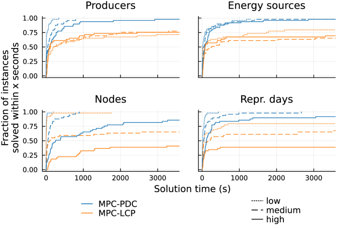
Figure 2: Cumulative distribution functions of solution times for the two formulations with 1-3 producers, 4-6 energy sources and 2-4 nodes and representative days. For each problem size, 50 instances are generated and solved.

In the instances in Figure 1, the value of the top-level decision variable $\rho$ is always zero. This suggests that in this specific problem, there is no need for the top-level player to impose a constraint (13d) in the middle-level problem. Furthermore, this means that there are no conflicts between the top- and middle-level objectives such that the middle-level player would select a low-renewable bottom-level equilibrium that the top-level player would disagree with.

4.2 Case study: a five-node Nordic energy system

The case study in [6] considers five nodes, representing Finland, Sweden, Norway, Denmark and the combined Baltic countries (Estonia, Latvia and Lithuania). There are five producers, each owning production capacity in one of the five nodes. Nine different energy sources are available, consisting of five conventional sources: nuclear, coal, gas (closed- and open-cycle) and biomass, and four renewable sources: solar, hydro, onshore and offshore wind. Additionally, we consider three representative days of renewable generation availability factors and demand curves. Recall that in our model, the top-level regulator makes their decisions independent of the day considered, that is, the carbon tax and minimum renewable share are constant across different representative days. These representative days are obtained in [6] by performing hierarchical clustering on demand, price and renewable availability data.

Day 1 is a winter day with higher demand, low solar availability and medium wind availability. Days 2 and 3 have a lower demand with day 2 representing a windy day with medium solar availability, and day 3 representing a sunny day with low wind availability. The details of the hierarchical clustering process can be found in [6].

We solve the problem with different values of the top-level objective weight $r$ to obtain a set of Pareto optimal solutions minimising emissions and maximising the value of production. For nonconvex problems, the weighting method does not necessarily find all Pareto optimal solutions [29]. Therefore, we also solve the problem with fixed values of the carbon tax $x$ (using $r=0.01$) to obtain a better understanding of the effect of a carbon tax between 0 and 19 €/ton, that is, the Pareto solutions that are not found by the weighting method. Fixing the $x$-variable results in a restricted version of the problem, allowing us to observe the effect of the carbon tax with values between the solutions found by the weighting method. Based on the results in Section 4.1, we represent the trilevel problem using the MPC-PDC reformulation.

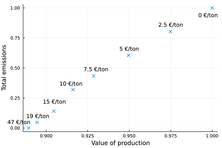
Figure 3: Some Pareto optimal solutions to the Nordic case study, and the associated carbon tax values $x$. The total production and emissions are scaled such that value 1 corresponds to a solution without a carbon tax.

In Figure 3, we can see the shape of the Pareto frontier. With a carbon tax of 47 €/ton, the system produces no emissions, and the total value of production is decreased by 11.1% from the top-right corner where the carbon tax is zero and the value of production is at its maximum. The emissions are almost completely removed from the system with a carbon tax of 19 €/ton, but removing the last emissions requires a large increase in tax. We also observe that the weighting method does not find the solutions with a carbon tax between 0 and 19 €/ton. This is an interesting result suggesting that in this case study, slightly decreasing the carbon tax from 19 €/ton increases emissions quickly relative to the increase in the total value of production.

In Figure 4, the production portfolio (a weighted average over the representative days, using the distribution in [6]) is presented for a model with no carbon tax (i.e., regulator heavily prefers maximising production over minimising emissions) and a carbon tax of 19 €/ton (enough to remove nearly all emissions). We can see that because of the substantial hydropower production capacity in the Nordic system, particularly in Norway and Sweden [23], the renewable share of production is large even without a carbon tax. The only significant source of emissions seems to be coal, and introducing a carbon tax of 19 €/ton removes nearly all coal from the portfolio, bringing in a small amount of closed-cycle gas power instead. The closed-cycle gas production occurs in the Baltics in day 1, and to understand this emergence of gas better, we must examine the transmission network in Figure 5.

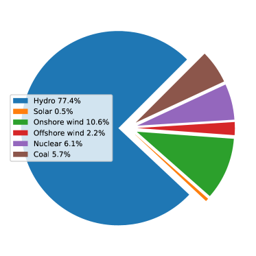
(a)

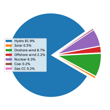
(b)

Figure 4: Weighted average electricity production portfolio over the five nodes and three representative days.

The first representative day has the highest network usage with large amounts of electricity transmitted from Norway to Finland through Sweden. With the carbon tax, the importance of transmission is further highlighted as the hydropower capacity in Norway is used for lowering overall prices under high demand and low production. The differences between representative days 2 and 3 are more subtle, but we can see, e.g., the reliance on wind power in Denmark: in the low-wind day 3, the carbon tax results in Denmark importing a significant amount of electricity from Norway, compared to the high-wind day 2. In the first day with a carbon tax of 19 €/ton, both lines connecting the Baltic countries to the rest of the system are at their capacity, explaining why the Baltic countries start using gas power after a carbon tax is introduced. This illustrates the complex interplay between the three levels that is captured by our model.

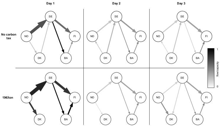
Figure 5: Transmission grid usage with different carbon taxes and representative days. The size of an arrow is proportional to the flow on the line and the color of an arrow represents congestion: black arrows correspond to lines operating at their limit. The nodes are FI=Finland, SE=Sweden, NO=Norway, DK=Denmark, BA=Baltic countries.

5 Conclusions

In this paper, we propose a trilevel optimisation framework for energy systems planning with environmental considerations. Additionally, we characterise the notion of weak and strong trilevel structures and compare two single-level reformulations for problems with a weak trilevel structure. The two formulations are the MPC-LPC reformulation, originally presented in [15], and the MPC-PDC reformulation, an original development in this paper.

The computational results are encouraging, as we are able to solve the case study to optimality within a few minutes. However, we note that seemingly small extensions to the model, such as adding ramping constraints (limiting the change in production between consecutive periods) to the producer problem could increase the complexity of the model enough to make the problem computationally intractable. For the results in this paper, an off-the-shelf solver is used, which is useful to ensure a low barrier-to-entry for using the developed formulation. However, we believe that the computational performance can be increased considerably using specialised solution methods. The model could also be extended to consider transmission and/or production capacity expansion over multiple timesteps, especially if computationally more efficient reformulations and solution methods are found.

A limitation of the solution methods presented in this paper is that they require a weak trilevel structure. In practice, many relevant problems will have a strong trilevel structure, precluding the use of these reformulations. Thus, further research is needed on developing (heuristic) solution methods for problems with a strong trilevel structure. Notably, ideas such as bilevel branch-and-bound [13] and convex hull reformulations of the middle-level feasible region [33] should be explored in the context of the problems presented in this paper.

Appendix A Reformulation of a bottom-level LCP with a positive semi-definite M

[9] shows that if the matrix $M$ is positive semidefinite, all solutions to the LCP

$$0\leq z\perp q+N_{x}x+N_{y}y+Mz\geq 0,$$ (24)

can be obtained as the following polyhedral set:

$$\{z\in R^{n_{z}}_{\geq 0}: \ q+N_{x}x+N_{y}y+Mz\geq 0,$$

$$\ (q+N_{x}x+N_{y}y)^{T}(z-\bar{z})=0,$$ (25)

$$\ (M+M^{T})(z-\bar{z})=0\},$$

where $\bar{z}$ is a solution to the LCP.

Hence, the middle-level problem can be re-written as

$$min_{y,z\geq 0}\quad d_{2}^{\top}y+e_{2}^{\top}z$$ (26a)

$$s.t.\quad A_{2}x+B_{2}y+C_{2}z\geq a_{2}$$ (26b)

$$q+N_{x}x+N_{y}y+Mz\geq 0$$ (26c)

$$(q+N_{x}x+N_{y}y)^{\top}(z-\bar{z})=0$$ (26d)

$$(M+M^{\top})(z-\bar{z})=0.$$ (26e)

We observe that (26d) includes a bilinear term $y^{\top}N_{y}^{\top}z$ in an equality constraint. This is a nonconvex constraint, precluding the direct use of KKT conditions for obtaining an optimal solution to (26). However, for problems with a weak tri-level structure, $N_{y}=0$ and these bilinear terms vanish. In the next theorem, we assume $N_{y}=0$.

Theorem A.1.

Let $M$ be a positive semidefinite matrix. Then, $(x^{*},y^{*},z^{*})$ is an optimal solution of Problem (3) with middle level (4) if and only if $(x^{*},y^{*},z^{*},\bar{z}^{*})$ is an optimal solution of the problem

$$min_{x,y,z,\bar{z}}\quad c_{1}^{\top}x+d_{1}^{\top}y+e_{1}^{\top}z$$ (27a)

$$s.t.\quad A_{1}x+B_{1}y+C_{1}z\geq a_{1}$$ (27b)

$$\bar{z}\in\operatorname*{arg\,min}_{z^{\prime}\geq 0}\{{z^{\prime}}^{\top}(q+N_{x}x+M{z^{\prime}}):$$

$$\qquad\qquad\quad q+N_{x}x+M{z^{\prime}}\geq 0\quad(\beta)\},$$ (27c)

$$y,z\in\operatorname*{arg\,min}_{\hat{y},\hat{z}\geq 0}\{d_{2}^{\top}\hat{y}+e_{2}^{\top}\hat{z}:$$

$$\qquad\qquad q+N_{x}x+M\hat{z}\geq 0\quad(\delta)$$

$$\qquad\qquad(q+N_{x}x)^{\top}(\hat{z}-\bar{z})=0\quad(\zeta)$$ (27d)

$$\qquad\qquad(M+M^{\top})(\hat{z}-\bar{z})=0\quad(\eta)$$

$$\qquad\qquad A_{2}x+B_{2}\hat{y}+C_{2}\hat{z}\geq a_{2}\quad(\gamma)\},$$

$$\text{such that }(\bar{z}^{*})^{\top}(q+N_{x}x^{*}+M\bar{z}^{*})=0.$$

See Theorem 6 in [15] for a proof of this result as well as related theoretical aspects of the general form of the problem.

The two nested optimization problems in (27) are a convex QP (27c) and an LP (27d). Hence, the KKT conditions of both problems are necessary and sufficient for optimality and the two inner problems can be replaced by their necessary and sufficient KKT conditions, leading to the single-level reformulation (6).

Appendix B Formulating the dual of a QP with affine constraints

Given a quadratic program with affine constraints

$$\min_{z_{i}}\quad \frac{1}{2}z_{i}^{\top}F_{i}z_{i}+e_{i3}(x)^{\top}z_{i}$$ (28a)

s.t. $$C_{i3}z_{i}\geq a_{i3}(x)\quad(p_{i})$$ (28b)

$$z_{i}\geq 0\quad(s_{i}),$$ (28c)

where we assume $F_{i}$ is a positive semidefinite symmetric matrix, the Lagrangian of the problem is

$$L(z_{i},s_{i},p_{i})=\frac{1}{2}z_{i}^{\top}F_{i}z_{i}+e_{i3}(x)^{\top}z_{i}+p_{i}^{\top}(a_{i3}(x)-C_{i3}z_{i})-s_{i}^{\top}z_{i},$$ (29)

where $p_{i}$ and $s_{i}$ are nonnegative Lagrange multipliers or dual variables. The first-order optimality condition is thus

$$\nabla_{z_{i}}L(z_{i},s_{i},p_{i})=F_{i}z_{i}+e_{i3}(x)-C_{i3}^{\top}p_{i}-s_{i}=0$$ (30)

and rearranging (29) gives us

$$\frac{1}{2}z_{i}^{\top}F_{i}z_{i}-z_{i}^{\top}C_{i3}^{\top}p_{i}+z_{i}^{\top}e_{i3}(x)-z_{i}^{\top}s_{i}+a_{i3}(x)^{\top}p_{i},$$ (31)

which, using the first order condition $-F_{i}z_{i}=-C_{i3}^{\top}p_{i}+e_{i3}(x)-s_{i}$, becomes

$$-\frac{1}{2}z_{i}^{\top}F_{i}z_{i}+a_{i3}(x)^{\top}p_{i}.$$ (32)

Maximizing Eq. (32), subject to the first-order optimality condition for $z_{i}$ and treating $s_{i}$ as a slack variable and removing its explicit representation from the problem results in the Lagrangian dual formulation

$$\max_{p_{i},z_{i}}\quad -\frac{1}{2}z_{i}^{\top}F_{i}z_{i}+a_{i3}(x)^{\top}p_{i}$$ (33a)

s.t. $$C_{i3}^{\top}p_{i}-F_{i}z_{i}\leq e_{i3}(x)$$ (33b)

$$p_{i}\geq 0.$$ (33c)

Appendix C Solving for the arbitrage amounts and hub prices in the arbitrage model

We have the necessary and sufficient KKT conditions

$$\alpha_{k}-\beta_{k}(\sum_{i^{\prime}\in I}s_{i^{\prime}k}+a_{ik})=p_{Hi}+w_{k}\forall k\in K$$ (34)

$$\sum_{k\in K}a_{ik}=0$$ (35)

of the arbitrager’s problem, and with the substitution $\sum_{j\in J}z_{ijk}=s_{ik}$, we get

$$\alpha_{k}-\beta_{k}(Z_{k}+a_{ik})=p_{Hi}+w_{k}\forall k\in K$$ (37)

$$\sum_{k\in K}a_{ik}=0,$$ (38)

where $Z_{k}=\sum_{i\in F,j\in J}z_{ijk}$. In matrix form, we get

$$\begin{bmatrix}Q&\mathbf{1}\\ \mathbf{1}^{\top}&0\end{bmatrix}\begin{bmatrix}a_{i}\\ p_{Hi}\end{bmatrix}=\begin{bmatrix}\alpha-QZ-w\\ 0\end{bmatrix},$$ (40)

where Q is a square diagonal matrix with the element on the $k$th row and column being $\beta_{k}$ and $\mathbf{1}$ is a vector of ones. It can be shown that

$$\begin{bmatrix}Q&\mathbf{1}\\ \mathbf{1}^{\top}&0\end{bmatrix}^{-1}=\begin{bmatrix}L&d\\ d^{\top}&\hat{d}\end{bmatrix},$$ (41)

where

$$\hat{d} =\frac{1}{\sum_{k\in K}\beta_{k}^{-1}}$$

$$d_{k} =\beta_{k}^{-1}\hat{d}$$

$$L_{k,k} =\hat{d}\beta_{k}^{-1}\sum_{k^{\prime}\in K\setminus k}\beta_{k}^{\prime-1}$$

$$L_{k,k^{\prime}} =-\hat{d}\beta_{k}^{-1}\beta_{k}^{\prime-1},\ k\neq k^{\prime}.$$

This results in the solution

$$a_{ik} =d_{k}Z-Z_{k}-\sum_{k^{\prime}\in K}(\alpha_{k^{\prime}}-w_{k^{\prime}})L_{k,k^{\prime}}$$ (42)

$$p_{Hi} =\sum_{k\in K}(\alpha_{k}-w_{k})d_{k}-Z\hat{d},$$ (43)

where

$$Z =\sum_{i\in I,j\in J,k\in K}z_{ijk}$$

$$Z_{k} =\sum_{i\in I,j\in J}z_{ijk}.$$

It can be seen that the values of $a_{ik}$ and $P_{Hi}$ are the same for each firm $i\in I$ and we can drop the index $i$. [8] shows that the arbitrage amounts correspond to the transmission values: $a_{k}=y_{k}$. With some algebra, we can see that the hub price $p_{H}$ can be represented as a weighted sum of the node prices excluding transmission. Given the solution

$$p_{H}=\sum_{k\in K}(\alpha_{k}-w_{k})d_{k}-Z\hat{d},$$

we can rearrange the terms to get

$$p_{H}=\hat{d}\sum_{k\in K}(\frac{\alpha_{k}-w_{k}}{\beta_{k}}-Z_{k}).$$

If we now denote $d^{\prime}_{k}=\prod_{k^{\prime}\in K\setminus k}\beta_{k^{\prime}}$, we get $\hat{d}=\frac{\prod_{k\in K}\beta_{k}}{\sum_{k\in K}d^{\prime}_{k}}$, and including the nominator in the price term in the hub price formula, we get

$$p_{H}=\frac{\sum_{k\in K}(\alpha_{k}-\beta_{k}Z_{k}-w_{k})d^{\prime}_{k}}{\sum_{k\in K}d^{\prime}_{k}}$$

or equivalently

$$p_{H}=\sum_{k\in K}\frac{d^{\prime}_{k}}{\sum_{k\in K}d^{\prime}_{k}}(\alpha_{k}-\beta_{k}Z_{k}-w_{k}).$$

Finally, we observe that $d_{k}=\frac{d^{\prime}_{k}}{\sum_{k\in K}d^{\prime}_{k}}$, and we get

$$p_{H}=\sum_{k\in K}d_{k}(\alpha_{k}-\beta_{k}Z_{k}-w_{k}).$$

Appendix D Including variability in the model

To make our problem setting slightly more realistic, we consider a set of representative days for renewable energy availability and demand. These scenarios (also known as representative days) are obtained in [6] by using hierarchical clustering. The top-level problem becomes (44) where the objective function becomes the expected value of the objective of (12) over the set of representative days $s\in S$. For the system operator (45) and the producers (46), the same problems as before are solved separately for each $s\in S$, implying that the system operator and producers make their operating decisions based on the operating conditions, while the regulator chooses a tax that is used in all scenarios. This makes sense from a practical standpoint, as electricity production and transmission should depend on the demand and renewable energy availability, and a high-level decision such as carbon tax should be a constant to make it clear for the players.

$$\max_{x,y,z}\quad \sum_{s\in S}P(s)\sum_{i\in I,j\in J,k\in K}(r\theta_{ijk}-(1-r)\eta_{ijk})z_{ijks}$$ (44a)

s.t. $$x\geq 0$$ (44b)

$$0\leq\rho\leq 1$$ (44c)

$$z_{s}\text{ and }y_{s}\text{ solve }\eqref{eq:profit_iso-stoch}\text{ for all }s\in S.$$ (44d)

$$\max_{y_{ks},z_{ijks}}\quad \sum_{k\in K}w_{ks}y_{ks}$$ (45a)

s.t. $$-\sum_{k\in K}PTDF_{ka}y_{ks}\leq T_{a}^{-}\quad(\phi_{as}^{-})\ \forall a\in A$$ (45b)

$$\sum_{k\in K}PTDF_{ka}y_{ks}\leq T_{a}^{+}\quad(\phi_{as}^{+})\ \forall a\in A$$ (45c)

$$\sum_{i\in I,j\in R}z_{ijks}\geq\rho\sum_{i\in I,j\in J}z_{ijks}\quad(\psi_{ks})\ \forall k\in K$$ (45d)

$$z_{ijks}\text{ solve }\eqref{eq:bottom-level-primal-arbitrage-reduced-stoch}\text{ for all }i\in I\text{ and for }s,$$ (45e)

$$\max_{z_{ijks}}\quad \left(\sum_{k\in K}(\alpha_{ks}-w_{ks})d_{ks}-Z_{s}\hat{d}_{s}\right)Z_{is}-\sum_{j\in J,k\in K}\left(\gamma_{ijk}-w_{ks}\right)z_{ijks}$$ (46a)

s.t. $$z_{ijks}\leq z_{ijks}^{max}\quad(\lambda_{ijks})\ \forall j\in J,k\in K$$ (46b)

$$z_{ijks}\geq 0\ \forall j\in J,k\in K$$ (46c)

References

- [1] Jonathan F Bard “An algorithm for solving the general bilevel programming problem” In Mathematics of Operations Research 8.2 INFORMS, 1983, pp. 260–272 DOI: https://doi.org/10.1287/moor.8.2.260
- [2] Jonathan F Bard “Some properties of the bilevel programming problem” In Journal of optimization theory and applications 68.2 Springer, 1991, pp. 371–378
- [3] Luis Baringo and Antonio J Conejo “Transmission and wind power investment” In IEEE transactions on power systems 27.2 IEEE, 2012, pp. 885–893
- [4] Mokhtar S Bazaraa, Hanif D Sherali and Chitharanjan M Shetty “Nonlinear programming: theory and algorithms” John Wiley & Sons, 2013
- [5] Evelyn Martin Lansdowne Beale and John A Tomlin “Special facilities in a general mathematical programming system for non-convex problems using ordered sets of variables” In OR 69.99, 1970, pp. 447–454
- [6] Nikita Belyak, Steven A. Gabriel, Nikolay Khabarov and Fabricio Oliveira “Optimal transmission expansion planning in the context of renewable energy integration policies” arXiv, 2023 DOI: 10.48550/ARXIV.2302.10562
- [7] Jeff Bezanson, Alan Edelman, Stefan Karpinski and Viral B Shah “Julia: A fresh approach to numerical computing” In SIAM Review 59.1 SIAM, 2017, pp. 65–98 DOI: 10.1137/141000671
- [8] Carolyn Burr Metzler “Complementarity models of competitive oligopolistic electric power generation markets”, 2000
- [9] Richard W. Cottle, Jong-Shi Pang and Richard E. Stone “The Linear Complementarity Problem” Society for IndustrialApplied Mathematics, 2009 DOI: 10.1137/1.9780898719000
- [10] William S Dorn “Duality in quadratic programming” In Quarterly of applied mathematics 18.2, 1960, pp. 155–162
- [11] Iain Dunning, Joey Huchette and Miles Lubin “JuMP: A Modeling Language for Mathematical Optimization” In SIAM Review 59.2, 2017, pp. 295–320 DOI: 10.1137/15M1020575
- [12] Francisco Facchinei and Christian Kanzow “Generalized Nash equilibrium problems” In Annals of Operations Research 175.1 Springer, 2010, pp. 177–211
- [13] Matteo Fischetti, Ivana Ljubić, Michele Monaci and Markus Sinnl “On the use of intersection cuts for bilevel optimization” In Mathematical Programming 172.1-2 Springer, 2018, pp. 77–103
- [14] Steven A Gabriel et al. “Complementarity Modeling in Energy Markets” Springer Science & Business Media, 2012
- [15] Steven A. Gabriel, Marina Leal and Martin Schmidt “On linear bilevel optimization problems with complementarity-constrained lower levels” In Journal of the Operational Research Society 73.12 Taylor & Francis, 2022, pp. 2706–2716 DOI: 10.1080/01605682.2021.2015254
- [16] Yan Gu, Xingju Cai, Deren Han and David ZW Wang “A Tri-level Optimization Model for a Private Road Competition Problem with Traffic Equilibrium Constraints” In European Journal of Operational Research 273.1 Elsevier, 2019, pp. 190–197
- [17] Gurobi Optimization, LLC “Gurobi Optimizer Reference Manual”, 2022 URL: https://www.gurobi.com
- [18] Miroslav Hájek, Jarmila Zimmermannová, Karel Helman and Ladislav Rozenskỳ “Analysis of carbon tax efficiency in energy industries of selected EU countries” In Energy Policy 134.110955 Elsevier, 2019
- [19] Olli Herrala “Source code repository for the trilevel models in this paper”, 2023 URL: https://github.com/solliolli/trilevel-energy
- [20] Benjamin F Hobbs “Linear complementarity models of Nash-Cournot competition in bilateral and POOLCO power markets” In IEEE Transactions on power systems 16.2 IEEE, 2001, pp. 194–202
- [21] Daniel Huppmann and Jonas Egerer “National-strategic investment in European power transmission capacity” In European Journal of Operational Research 247.1 Elsevier, 2015, pp. 191–203
- [22] Marija Ilic, Francisco Galiana and Lester Fink “Power systems restructuring: engineering and economics” Kluwer Academic Publishers, 1998
- [23] IRENA “Renewable capacity statistics 2023” In International Renewable Energy Agency, Abu Dhabi, 2023
- [24] Shan Jin and Sarah M Ryan “A Tri-level Model of Centralized Transmission and Decentralized Generation Expansion Planning for an Electricity Market—Part I” In IEEE Transactions on Power Systems 29.1 IEEE, 2013, pp. 132–141
- [25] William Karush “Minima of functions of several variables with inequalities as side conditions”, 1939
- [26] Thomas Kleinert, Martine Labbé, Ivana Ljubić and Martin Schmidt “A survey on mixed-integer programming techniques in bilevel optimization” In EURO Journal on Computational Optimization 9.100007 Elsevier, 2021
- [27] Harold W. Kuhn and Albert W. Tucker “Nonlinear Programming” In Berkeley Symposium on Mathematical Statistics and Probability 1951, 1951, pp. 481–492
- [28] Sven Leyffer et al. “A survey of nonlinear robust optimization” In INFOR: Information Systems and Operational Research 58.2 Taylor & Francis, 2020, pp. 342–373
- [29] Kaisa M. Miettinen “Nonlinear multiobjective optimization” Kluwer Academic Publishers, 1999
- [30] S Pineda, H Bylling and JM Morales “Efficiently solving linear bilevel programming problems using off-the-shelf optimization software” In Optimization and Engineering 19.1 Springer, 2018, pp. 187–211
- [31] Kris Poncelet et al. “Selecting representative days for capturing the implications of integrating intermittent renewables in generation expansion planning problems” In IEEE Transactions on Power Systems 32.3 IEEE, 2016, pp. 1936–1948
- [32] Carlos Ruiz, Antonio J Conejo and Yves Smeers “Equilibria in an oligopolistic electricity pool with stepwise offer curves” In IEEE Transactions on Power Systems 27.2 IEEE, 2011, pp. 752–761
- [33] Asteroide Santana and Santanu S Dey “The convex hull of a quadratic constraint over a polytope” In SIAM Journal on Optimization 30.4 SIAM, 2020, pp. 2983–2997
- [34] Sauleh Siddiqui and Steven A Gabriel “An SOS1-based approach for solving MPECs with a natural gas market application” In Networks and Spatial Economics 13 Springer, 2013, pp. 205–227
- [35] Ankur Sinha, Pekka Malo and Kalyanmoy Deb “A review on bilevel optimization: From classical to evolutionary approaches and applications” In IEEE Transactions on Evolutionary Computation 22.2 IEEE, 2017, pp. 276–295
- [36] Morton Slater “Lagrange Multipliers Revisited” In Cowles Foundation Discussion Papers 304, 1950
- [37] Jane J Ye and DL Zhu “Optimality conditions for bilevel programming problems” In Optimization 33.1 Taylor & Francis, 1995, pp. 9–27