Dynamic Early Exiting Predictive Coding Neural Networks

Abstract

Internet of Things (IoT) sensors are nowadays heavily utilized in various real-world applications ranging from wearables to smart buildings passing by agrotechnology and health monitoring. With the huge amounts of data generated by these tiny devices, Deep Learning (DL) models have been extensively used to enhance them with intelligent processing. However, with the urge for smaller and more accurate devices, DL models became too heavy to deploy. It is thus necessary to incorporate the hardware’s limited resources in the design process. Therefore, inspired by the human brain known for its efficiency and low power consumption, we propose a shallow bidirectional network based on predictive coding theory and dynamic early exiting for halting further computations when a performance threshold is surpassed. We achieve comparable accuracy to VGG-16 in image classification on CIFAR-10 with fewer parameters and less computational complexity.

I Introduction

The Internet of Things (IoT) is nowadays a paradigm of reference for several applications. IoT is adopted in various domains such as smart farming, drone imaging, industry 4.0, and safety and is implemented in many challenging environments like satellites, submarines, and the Large Hadron Collider (LHC). Hence, huge amounts of data are amassed by sensors and can be overwhelming to process. For example, the LHC generates approximately one petabyte of collision data per second [1]. Therefore, IoT sealed an alliance with Artificial Intelligence (AI) to improve data management pipelines and offer better analytics to clients. In the context of Artificial Intelligence of Things (AIoT), Deep Learning (DL) models, mainly fostered in cloud servers, have proven their efficacy in injecting intelligence into the network of connected IoT devices [2]. Raw data captured by sensors can thus be used to produce pertinent insights for the end user’s benefit.

With the rapid development of edge computing, AI services have known a migration from cloud servers to edge devices (e.g., IoT gateways and fog nodes). For sensitive applications, such as e-health and smart surveillance, deploying AI services at the edge has numerous benefits [3]. Data will no longer need to be transferred through the Internet, increasing data privacy and reducing security breaches. Latency will also be reduced to account only for the deployed models’ computational complexity. However, edge devices can span large computational resource constraints from microcontrollers to cloudlets passing by single-board computers [4]. Therefore, the observed heterogeneity in edge device requirements can be troublesome for deploying state-of-the-art DL models as they usually perform with very deep networks implicating large numbers of parameters, thus resulting in an inevitable increase in memory footprint and inference time.

To address this issue, an extensive body of work proposes various techniques of model compression for lighter memory footprints. For instance, quantization aims at coding weights on low-precision arithmetic and knowledge distillation allows the design of a small model (i.e., student) trained on quality features from a bigger network (i.e., teacher) [5]. Another avenue of research takes inspiration from the brain, known for its efficiency and plasticity.

The human brain is able to conduct a wide range of tasks dexterously and process huge amounts of data with around 20 Watts of power [6]. The brain’s neuronal morphology could explain this frugality in energy consumption. The brain relies on inhibitory mechanisms that are necessary for quick decision-making in a survivalist situation [7] as well as bidirectional connections between higher and lower visual areas that enhance the brain’s abstraction capacities of the surrounding environment [8]. To understand the interactions between both visual areas, predictive coding (PC) [9] theory postulates that the main function of the brain is to minimize a prediction error defined as the difference between the real and predicted stimuli. PC shows that feed-forward connections drive prediction errors to higher layers, whereas feedback connections attempt to predict lower layers’ neural activity. The bidirectional movement relies on continuously refining the brain’s internal input representations throughout the visual hierarchy. When implemented in convolutional neural networks (CNN), PC often yields higher accuracy than its conventional counterpart [10].

In light of these ideas, our goal is to benefit from PC in designing shallow CNNs. We aim to show empirically that the PC refinement process allows the same expressivity and feature diversity that width and depth allow in CNNs [11]. Furthermore, the refinement of feature representations demands a certain amount of cyclic processing between lower and higher visual areas until equilibrium is reached [12]. To alleviate this issue, early exiting techniques [13] are used to abort further cycling over the feature extractor network once a performance threshold is reached.

Our contributions can be formulated as follows:

• We apply PC techniques to CNNs to design shallow networks with a considerably reduced memory footprint that are deployable on edge devices

• We improve PC cyclic processing with an early-exiting mechanism which further reduces the computational cost and inference time

• We evaluate our proposed model against VGG-16 and achieve for image classification on CIFAR-10 comparable results with only a 3% difference and less than 1% of the baseline’s number of parameters

II Related Work

This section reviews the main research fields that intersect with our work. The section covers some solutions to deploy DL models on low-resource edge devices, previous work done on PC with DL models, and recent applications of early exiting techniques.

II-A DL for Resource-constrained Devices

When computations are fostered in one edge device, compression is a potential direction for obtaining smaller models. Compression encompasses various techniques that reduce the model size without a severe drop in performance. The two most prominent techniques are quantization and pruning. On the one hand, quantization is the process of representing the model’s weights, activations, or gradients with a lower number of bits either during or after training [14]. Rather than optimizing for a target bit-width, mixed quantization allows the model to be coded on longer bits for early feature extraction layers and shorter bits for intermediate or concatenation layers [15]. A recent line of work investigates binary neural networks whose parameters can be coded only on 2 bits [16]. On the other hand, pruning entirely removes weights from a network according to a predefined metric of importance. Thus, numerous metrics exist, such as weight magnitude or impact on loss [17]. These pruning criteria can either be applied to a pre-trained network, during training with the possibility of growing back connections, or even before training at initialization [18].

Instead of working on the model itself with one edge processor, another venue for deployment in resource-constrained hardware would consider the scenario where a heterogeneous network is formed via interconnected devices of different capabilities. Distributed inference [19] is a solution that leverages the power of internet-connected networks. Rather than deploying a heavy model on one device, we would cut the model into small executable segments on the variety of available devices within the network. However, this solution encounters privacy and latency challenges that Federated Learning has proposed to raise by avoiding data transfer between the network’s nodes and encouraging collaborative learning between the devices [20].

Our work complements the aforementioned techniques since our proposed models can further reduce their memory footprint and number of operations through quantization and pruning or be deployed in a distributed network.

II-B Deep Predictive Coding Networks

PredNet [21] was the first attempt to implement predictive coding in deep neural networks with the unsupervised task of next-frame video prediction. It uses multiple layers of recurrent convolutional Long Short-Term Memory cells that generate a prediction (next frame). This prediction is used to compute an error representation that is passed to the subsequent layers. However, the proposed architecture did not benefit from the power of predictive coding as it did not force the minimization of the bottom-up error [22].

In a supervised learning scheme, Wen et al. enhanced a conventional CNN with top-down deconvolutional layers using PC updates [10]. It was shown that a deep PC network yields higher performance than its homologous plain feed-forward network. Although the network was trained for one particular number of cycles ($T=6$), they reported a positive correlation between accuracy and cycling numbers. Finally, PC-based networks were also shown to improve the robustness of deep models against several types of noises and adversarial attacks [23]. In this study, pre-trained models were enhanced with feedback connections, and only the latter were trained.

Our paper is deeply inspired by the advancements in PC-based neural networks. So far, PC has been utilized to improve model accuracy or robustness by adding feedback connections to deep feed-forward networks, which causes the number of parameters to double, and thus the latency to increase. Since our concern is low-resource edge devices, we envision PC as a technique that might help build shallow (i.e., few layers and parameters) and expressive (i.e., unrolling the model through the PC refinement process) networks.

II-C Early Exiting Networks

The most straightforward implementation of dynamic neural networks is based on Early Exiting [13]. It involves mounting tiny decision blocks onto a backbone model to make quick decisions for easy inputs without resorting to the entire network. In image classification, the decision block is a tiny multi-layer perceptron classifier. Therefore, in an early-exit network, a response is returned if the classifier is sufficiently confident based on a performance target. Otherwise, the example is passed onto the subsequent layers for finer processing [24]. In natural language processing, early exiting is used during the decoding of transformer-based large language models through dynamic per-token exit decision-making [25].

The early-exiting halting mechanism introduces the concepts of ”easy” and ”hard” samples, which imply that easy samples should exit at earlier classifiers and harder samples could traverse the full network. If this is intuitive in image classification, other tasks like object detection need more precise definitions of sample hardness. Therefore, in [26], a sample for object detection is labeled ”easy” when the difference in loss (or mean average precision) between a shallow detector and a deep detector is small. Early exiting networks are conventionally trained either via scalarization (i.e., the weighted sum of the internal classifiers losses) or separate training (i.e., each classifier trained separately). However, both methods have limitations as scalarization might cause instabilities due to the accumulation of gradients when the backbone is deep [27], while separate training hinders the collaboration between classifiers leading to computational waste [28].

In the proposed models, early exiting is implemented to halt PC cyclic processing once the user-defined performance target is reached.

III Proposed Architecture

As shown in Figure 1, our architecture is formed of a shared backbone alongside downstream task classifiers. The backbone serves as a feature extractor. It is built with a bidirectional hierarchy of convolutional and deconvolutional layers. The backbone is executed for a maximum of $T$ cycles before outputting the final feature vector for classification. Blue arrows represent the convolutional forward pass, while red arrows represent the feedback deconvolutions. Each intermediate representation consists of a concatenation of a convolutional and a deconvolutional feature maps, referred to as $C_{l}$ and $D_{l}$ respectively. We perform a variable number of cycles $t<T$ over the backbone. Once cycling is finished, we feed the last obtained feature vector $C_{l}(t)$ to the classifier corresponding to the achieved number of cycles $t$ (green arrow in Figure 1). The first cycle consists of three consecutive passes: forward, feedback, and forward. Every other cycle starts with a feedback pass followed by a forward pass.

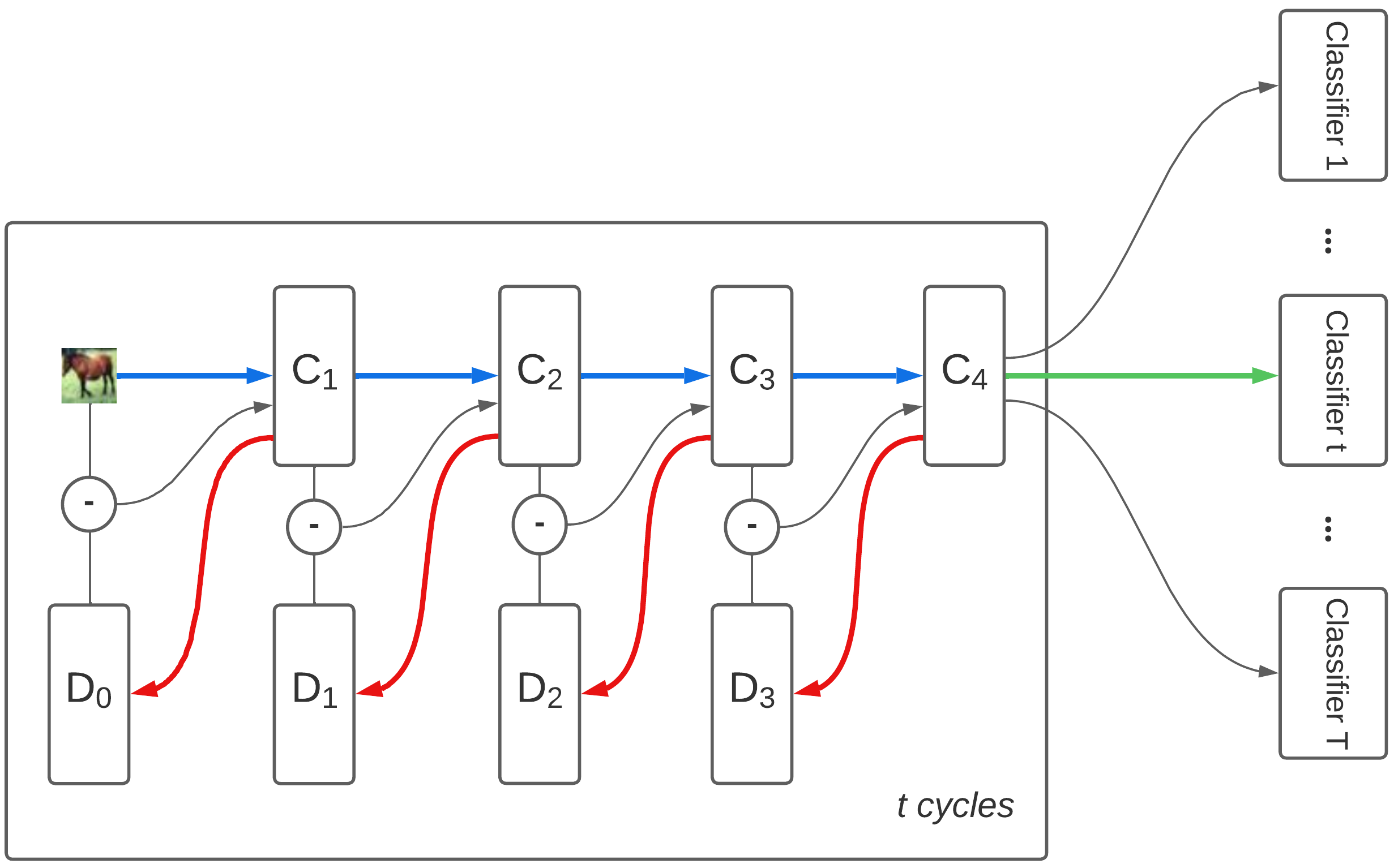
Figure 1: Proposed model - The backbone is cycling for $t<T$ cycles

III-A PC Feature Update Rule

During each cycle, PC adopts a specific feature update rule to merge forward and feedback feature maps to enrich the internal representation. We adopt the same formulation proposed in [10]. Suppose the PC architecture is constituted of $L$ layers, with layer $l=0$ being the input image. We denote the forward and feedback convolutions by $\mathbf{FF}$ and $\mathbf{FB}$. The convolutional representations $C_{l}$ are updated on both forward and feedback passes, while the deconvolutional feature maps $D_{l}$ only change during the feedback pass. Hence, let $C_{l,f}(t)$ and $C_{l,b}(t)$ be the state of layer $l$’s convolutional feature map at the end of the forward and feedback passes of PC cycle $t\in[|1,T|]$. At the beginning of cycle 1, we initialize all feature maps with a conventional forward pass: $\forall l\in[|1,L|],C_{l,f}(0)=\mathbf{FF}\left[C_{l-1,f}(0)\right]$. We can thus define the PC update rules for every cycle $t\in[|1,T|]$ and for every layer $l\in[|1,L|]$ as follows:

Feedback pass update:

$$D_{l-1}(t)=\mathbf{FB}(C_{l,f}(t-1))$$ (1)

$$C_{l-1,b}(t)=g((1-b_{l-1}).C_{l-1,f}(t-1)+b_{l-1}.D_{l-1}(t))$$

Forward pass update:

$$C_{l,f}(t)=g(C_{l,b}(t)+a_{l}.\mathbf{FF}(C_{l-1,b}(t)-D_{l-1}(t)))$$ (2)

where $a_{l}$ and $b_{l}$ are trainable non-negative layer-dependent updating rates, initialized for all layers by 1.0 and 0.5, respectively. However, $b_{0}=0$ is non-trainable as the input image $C_{0}$ is never updated. Finally, function $g$ is a Rectified Linear Unit (ReLU) non-linearity.

The PC update rules attempt to minimize the prediction error between forward and feedback representations. More precisely, after an optimal number of cycles $T_{opt}$, we will have $C_{l}(t)\simeq D_{l}(t)$. PC update rules thus tend toward a consistent feature representation: $\forall l\in[|1,L|],C_{l}(t+1)\simeq C_{l}(t)$. However, this condition is not always met in practice as it depends on the hardness of the sample being processed. For instance, hard images might require high cycling numbers to stabilize representations. Therefore, we do not wait until feature consistency is achieved to halt the computations as proposed explicitly in [23]. Instead, we propose to use early exiting to adapt the number of cycles to the sample hardness.

III-B PC Early Exit

We implement early exit on the number of cycles as follows. After the first cycle, classifier $1$ is applied to the convolutional feature map $C_{l,f}(1)$. The classification confidence is then compared with a predefined user threshold. If the confidence is above the threshold, computations are aborted, and a response is returned. Otherwise, a new cycle is initiated, followed by another classification and threshold comparison.

In the proposed architecture, the number of classifiers equals the maximum number of cycles $T$ allowed. The choice of $T$ different classifiers, instead of one classifier shared by all cycles, is motivated by the fact that feature vectors are updated from one cycle to another. Hence, a classifier trained on a 5-cycle-model feature vector will not discern the patterns that a 1-cycle-model extracts from the same input. Only when feature consistency is achieved can a shared classifier be sufficient. Nevertheless, since our target hardware is highly resource-constrained, we usually stop cycling before consistent feature representations are reached, hence the need for a classifier for each cycle.

III-C PC Training

Our model parameters are the forward, feedback, and the $T$ classifiers’ weights, alongside the $a_{l}$ and $b_{l}$ update rates. These parameters are learned with classic back-propagation using a single cross-entropy loss function $\mathcal{L}_{c_{i}}$ per classifier $c_{i}$. Hence, we can train the network separately for a specific number of cycles corresponding to one of the classifiers. Moreover, after each backpropagation pass, the weights are frozen until the chosen number $i$ of PC cycles is achieved before recalculating the loss function.

To improve the training performance, we can allow classifiers to collaborate with each other. Therefore, we propose that the backbone and $T$ classifiers are jointly trained using scalarization adopted from multi-objective optimization. The total loss is the weighted sum of each classifier’s loss $\mathcal{L}_{c_{i}}$, as defined in Equation 3:

$$\mathcal{L}_{tot}=\sum_{i=1}^{T}\lambda_{i}\mathcal{L}_{c_{i}}$$ (3)

where $\lambda_{i}$ is a positive weight for the loss function $\mathcal{L}_{c_{i}}$.

Our proposed training procedure has the main disadvantage of being time-consuming. However, not only does the underlying competition launched between classifiers over the shared weights of the backbone help achieve a Pareto optimal solution, but it also encourages PC cycles to achieve consistency early enough as the loss guides the classifiers to collaborate in generating semantically similar feature vectors. Moreover, the $\lambda_{i}$ coefficients control the exiting strategy: higher coefficients for the first classifiers (corresponding to small numbers of cycles) stimulate early exiting, and vice versa. In our experiments, exits were uniformly weighted: $\forall i\in[|1,T|],\lambda_{i}=1/T$.

IV Experiments

TABLE I: Model configurations

A	B	C
Input image 32x32
Conv-16	Conv-32	Conv-16
Conv-32	Conv-64	Conv-32
Conv-32	Conv-64	Conv-32
Conv-64	Conv-128	Conv-64
Conv-64	Conv-128	Conv-64
-	-	Conv-128
-	-	Conv-128
Global Average Pooling
$T$ Fully Connected layers

IV-A Dataset

In order to evaluate our method, we choose the CIFAR-10 dataset [29]. It includes 60000 32x32 RGB images evenly distributed over 10 classes, with 6000 images per each. CIFAR-10 is adopted by many tiny machine learning benchmarks [30], and the images simulate well numerous IoT applications using low-resolution cameras (e.g., surveillance for eyewear protection detection and smart farming for fruit disease classification). For model learning, the training set is formed of 50000 images, and the rest is destined for testing. As a data augmentation procedure, we applied random translation and horizontal flipping. The training set was clustered in 64-sized batches.

IV-B Training & Evaluation

We choose to cycle over the PC backbone for a maximum of $T=5$ cycles. Mini-batch gradient descent was employed for training via AdamW optimizer initialized with a learning rate of 0.001 and a weight decay of 0.01. Regularization was used as a dropout operator of 10%. We run the model for 500 epochs. Moreover, PC models with one cycling number and one classifier were trained for 200 epochs.

We adopt conventional accuracy as a performance metric for evaluation since the dataset is balanced. The number of parameters, memory size, and number of floating-point operations (FLOPs) can be gathered from PyTorch libraries. Latency was computed for one sample on Google Colaboratory CPU with 500 repetitions in the worst-case scenario (i.e., a sample exiting after all $T=5$ cycles), as it represents the upper bound of our setting.

IV-C Model configuration

The model design process was driven by the motivation of exploiting PC dynamics in order to build shallow networks, in terms of both depth and width, that could perform as well as the established VGG-16 architecture and that could be deployed on edge devices of kilobytes (KB) to megabytes (MB) of memory. We design three models with convolutions sharing the same kernel size of 3x3 and stride of 1 but different numbers of channels as shown in bold in Table I. For the sake of readability, we omit PC deconvolutional layers since they have inverted numbers of channels with respect to the feed-forward convolutions. Batch normalization is embedded in each convolutional block. Max-pooling of kernel size 2x2 is activated when the number of channels changes from one layer to another.

The models presented in Table I are designed to challenge PC feature updates. Hence, given a shallow Model A, we construct Model B to be wider and Model C deeper in order to show empirically that recurrence could account for the improvements that width and depth bring to the neural network. Finally, our baselines are VGG-16 as well as PC models exclusively trained for $T=5$ cycles with the aforementioned architectures in Table I, noted PCN-5-{A,B,C}. The custom baseline models PCN-5 are meant to testify to the validity of the chosen training scheme.

V Discussion

TABLE II: Characteristics for VGG-16 and $T=5$ processing cycles for the proposed models

Model	#Params	Size (MB)	FLOPs	Latency (ms)
VGG-16	134M	512.3	$8.7\times 10^{8}$	55.900
A	143.416	0.6	$3.3\times 10^{8}$	41.438
B	563.256	2.3	$1.05\times 10^{9}$	80.261
C	590.328	2.4	$4.9\times 10^{8}$	54.888

Table II and III aggregate the main results of our experiments from both efficiency and performance standpoints, respectively.

We observe that the proposed models can fit memory constraints for many edge processors consuming only a few megabytes of storage. As expected, latency and the number of operations increase with the model width and depth without exceeding the reasonable amounts we encounter in edge processing [4]. It is worth mentioning for Model B that a latency of 80 milliseconds (ms) is rather acceptable knowing that the network has already done 5 cycles through the backbone and computed 5 class probabilities, thus, offering better performance and more accurate classification. Based on Table II and Figure 2, Model A presents the most desirable properties for an edge application. It is noticeable that starting from cycle $T=2$, a linear relationship is found between cycles and FLOPs. It is explained by the fact that one more cycle implies the same amount of floating point operations. However, it is to note that the first cycle computes 2 feed-forward passes as the input should first traverse the network, feedback, and regain again the higher layers near the classifier. More cycles will thus grow the number of FLOPs linearly. However, given that our architecture is shallow, attaining reasonably large numbers of cycles will barely reach the computational cost attained by a conventional deep network like VGG-16, as seen in the FLOPs column of Table II.

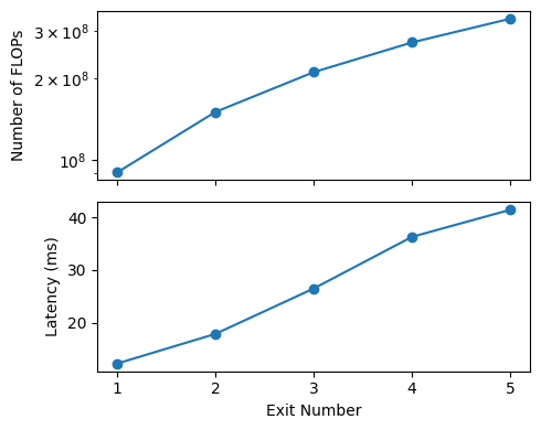
Figure 2: FLOPs and Latency on CPU across exits for Model A

From a performance perspective, we observe from Table III, an increasing accuracy through cycles as more cycles allow more expressivity to the shallow network. This is especially the case when classes are hardly separable and for which the learned patterns must be well distinctive. To appreciate the impact of PC updates, we note a significant increase of about 20% from $T=1$ to $T=5$ in Model B. Moreover, in order to challenge our training scheme, we report models trained for the predefined maximum number of cycles $T=5$ and one classifier. We observe that models using joint training achieve better accuracy than their homologous PCN-5. This shows that, in a PC setting for which consistency is sought, joint training encourages collaboration between classifiers. Furthermore, our proposed models are not very far from VGG-16 performance on CIFAR-10 with only a 3% difference from the 4-cycle and 5-cycle recurrent processing and a considerable reduction in the numbers of parameters from $10^{8}$ (i.e., VGG-16) to $10^{5}$ orders of magnitude.

Table III also shows comparable results between the three proposed models. Wide Model B and deep Model C reach almost the same performance as Model A which is tinier and faster. Nevertheless, it is worth mentioning that width helped the model gain high accuracy at later cycles and depth improved the internal classifiers’ average performance. Overall, we can conclude that PC dynamics might serve as a complementary key aspect for increasing model expressivity along with depth and width in feed-forward neural networks.

Figure 3 endorses the claims advanced in Section III-C. We can spot two main behaviors, other than the collective increase in accuracy which is the goal of multiobjective optimization. The first is the fluctuations through epochs which reveal the status of competition between the classifiers. These fluctuations are severely present in the first epochs since PC dynamics can still not find common ground between the feature vectors each cycle is outputting. The second behavior is also related to these fluctuations: we observe that, near the end of the optimization, the fluctuation amplitude diminishes and the five curves approach one another. This behavior is compatible with the underlying idea of PC dynamics in neural networks that revolves around stability and consistency in the feature representations. Therefore, with the joint training, a type of implicit knowledge distillation happens between the cycles. Hence, in numerous cases, a 1-cycle network will be able to yield a similar feature vector as a 6-cycle network; a property which is most wanted for reducing computational cost.

TABLE III: Accuracy (%) of baseline models and dynamic PC models at different exits

Model	$T=1$	$T=2$	$T=3$	$T=4$	$T=5$
VGG-16	93.25 [31]
PCN-5-A	85.55
PCN-5-B	87.53
PCN-5-C	89.88
A	79.82	85.83	88.81	89.99	89.81
B	70.21	80.9	86.72	89.85	90.82
C	87.79	89.53	90.2	90.26	89.68

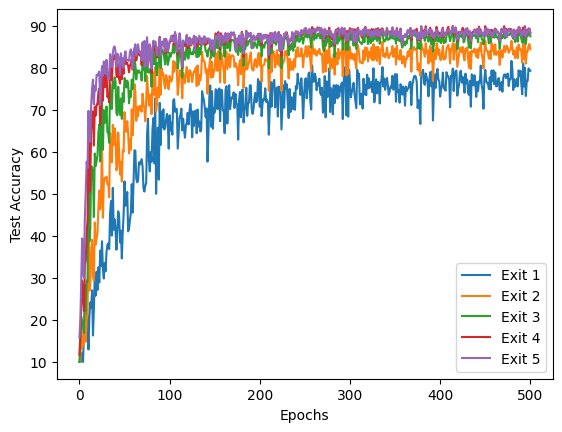
Figure 3: Test accuracy per exit for Model A

Finally, Figure 4 emphasizes the motivation behind using early exit. Given high thresholds, the network can still free with high confidence a large number of well-classified images at the first exit. Nevertheless, as the user threshold increases, we notice the importance of more cycles to classify harder samples correctly.

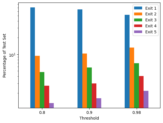
Figure 4: Ratio of correctly classified images exiting at different cycles based on a confidence threshold for Model A (ordinates in log scale)

VI Conclusion

In this paper, we proposed a shallow network for image classification based on predictive coding dynamics and early exiting for resource-constrained edge devices. We found that PC dynamics can play a major role in yielding high accuracy without resorting to deep models. Since PC is based on minimizing an objective function that might demand high numbers of cycles, we employed early-exiting to abort further computation once a user-predefined performance target is reached. Thus, the paper highlights how PC processing can lead to a significant reduction in memory footprint while achieving good accuracy. We intend to continue the present work by putting more emphasis on early exits through preference-vector-based multiobjective optimization. Furthermore, we will attempt to define a hardness measure that estimates beforehand the number of cycles needed in order to avoid calling low-cycle classifiers.

References

- [1] Stark, J, ”PLM and the Internet of Things,” Product Lifecycle Management, pp 327–352, vol. 1, Springer Cham., 2022.
- [2] T. J. Saleem and M. A. Chishti, ”Deep learning for the internet of things: Potential benefits and use-cases,” Digital Communications and Networks, vol. 7, no. 4, pp. 526–542, Nov. 2021.
- [3] R. Sanchez-Iborra and A. F. Skarmeta, ”TinyML-Enabled Frugal Smart Objects: Challenges and Opportunities,” in IEEE Circuits and Systems Magazine, vol. 20, no. 3, pp. 4-18, 2020.
- [4] M. G. S. Murshed, C. Murphy, D. Hou, N. Khan, G. Ananthanarayanan et al., ”Machine Learning at the Network Edge: A Survey,” ACM Comput. Surv., vol. 54, no. 8, p. 170:1-170:37, Oct. 2021.
- [5] J. Lee, L. Mukhanov, A. S. Molahosseini, U. Minhas, Y. Hua et al., ”Resource-Efficient Convolutional Networks: A Survey on Model-, Arithmetic-, and Implementation-Level Techniques,” ACM Comput. Surv., vol. 55, no. 13s, p. 276:1-276:36, Jul. 2023.
- [6] V. Balasubramanian, ”Brain power,” PNAS, vol. 118, no. 32, p. e2107022118, Aug. 2021.
- [7] L. Luo, ”Architectures of neuronal circuits,” Science, vol. 373, no. 6559, p. eabg7285, Sep. 2021.
- [8] C. J. Spoerer, T. C. Kietzmann, J. Mehrer, I. Charest, and N. Kriegeskorte, ”Recurrent neural networks can explain flexible trading of speed and accuracy in biological vision,” PLoS Comput Biol, vol. 16, no. 10, p. e1008215, Oct. 2020.
- [9] R. P. N. Rao and D. H. Ballard, ”Predictive coding in the visual cortex: a functional interpretation of some extra-classical receptive-field effects,” Nat. Neurosci., vol. 2, no. 1, Art. no. 1, Jan. 1999.
- [10] H. Wen, K. Han, J. Shi, Y. Zhang, E. Culurciello et al., ”Deep Predictive Coding Network for Object Recognition,” in Proceedings of ICML, Jul. 2018, pp. 5266–5275.
- [11] R. S. van Bergen and N. Kriegeskorte, ”Going in circles is the way forward: the role of recurrence in visual inference,” Current Opinion in Neurobiology, vol. 65, pp. 176–193, Dec. 2020.
- [12] Y. Song, T. Lukasiewicz, Z. Xu, and R. Bogacz, ”Can the Brain Do Backpropagation? — Exact Implementation of Backpropagation in Predictive Coding Networks,” in Advances in NeurIPS, 2020, pp. 22566–22579.
- [13] S. Laskaridis, A. Kouris, and N. D. Lane, ”Adaptive Inference through Early-Exit Networks: Design, Challenges and Directions,” Proceedings of EMDL’21, ACM, Jun. 2021, pp. 1–6.
- [14] A. Gholami, S. Kim, Z. Dong, Z. Yao, M. W. Mahoney et al., ”A Survey of Quantization Methods for Efficient Neural Network Inference,” in Low-Power Computer Vision, Chapman and Hall/CRC, 2022.
- [15] Z. Dong, Z. Yao, D. Arfeen, A. Gholami, M. W. Mahoney et al., ”HAWQ-V2: Hessian Aware trace-Weighted Quantization of Neural Networks,” in Advances in NeurIPS, 2020, pp. 18518–18529.
- [16] H. Qin, R. Gong, X. Liu, X. Bai, J. Song et al., ”Binary neural networks: A survey,” Pattern Recognition, vol. 105, p. 107281, Sep. 2020.
- [17] U. Evci, T. Gale, J. Menick, P. S. Castro, and E. Elsen, ”Rigging the lottery: making all tickets winners,” in Proceedings of ICML’20. pp. 2943–2952.
- [18] H. Wang, C. Qin, Y. Bai, Y. Zhang, and Y. Fu, ”Recent Advances on Neural Network Pruning at Initialization,” IJCAI, Jul. 2022, pp. 5638–5645.
- [19] J. Chen and X. Ran, ”Deep Learning With Edge Computing: A Review,” Proceedings of the IEEE, vol. 107, no. 8, pp. 1655–1674, Aug. 2019.
- [20] Y. Matsubara, M. Levorato, and F. Restuccia, ”Split Computing and Early Exiting for Deep Learning Applications: Survey and Research Challenges,” ACM Comput. Surv., vol. 55, no. 5, p. 90:1-90:30, Dec. 2022.
- [21] W. Lotter, G. Kreiman, and D. Cox, ”Deep Predictive Coding Networks for Video Prediction and Unsupervised Learning,” ICLR, Nov. 2016.
- [22] R. P. Rane, E. Szügyi, V. Saxena, A. Ofner, and S. Stober, ”PredNet and Predictive Coding: A Critical Review,” in Proceedings of ICMR ’20, ACM, Jun. 2020, pp. 233–241.
- [23] B. Choksi, M. Mozafari, C. Biggs O’ May, B. Ador, A. Alamia et al., ”Predify: Augmenting deep neural networks with brain-inspired predictive coding dynamics,” in Advances in NeurIPS, 2021, pp. 14069–14083.
- [24] S. Scardapane, M. Scarpiniti, E. Baccarelli, and A. Uncini, ”Why Should We Add Early Exits to Neural Networks?,” Cogn. Comput., vol. 12, no. 5, pp. 954–966, Sep. 2020.
- [25] T. Schuster, A. Fisch, J. Gupta, M. Dehghani, D. Bahri et al., ”Confident Adaptive Language Modeling,” in Advances in NeurIPS, May 2022.
- [26] Z. Lin, Y. Wang, J. Zhang, and X. Chu, ”DynamicDet: A Unified Dynamic Architecture for Object Detection,” Proceedings of the IEEE/CVF CVPR, 2023, pp. 6282–6291.
- [27] H. Li, H. Zhang, X. Qi, R. Yang, and G. Huang, ”Improved Techniques for Training Adaptive Deep Networks,” Proceedings of the IEEE/CVF ICCV, 2019, pp. 1891–1900.
- [28] M. Wołczyk, B. Wójcik, K. Bałazy, I. Podolak, J. Tabor et al., ”Zero Time Waste: Recycling Predictions in Early Exit Neural Networks,” in Advances in NeurIPS, 2021, pp. 2516–2528.
- [29] A. Krizhevsky, and G. Hinton, ”Learning Multiple Layers of Features from Tiny Images,” 2009.
- [30] C. Banbury, V. J. Reddi, P. Torelli, J. Holleman, N. Jeffries et al., ”MLPerf Tiny Benchmark,” Proceedings of the NeurIPS Track on Datasets and Benchmarks, 2021.
- [31] H. Jónsson, G. Cherubini, and E. Eleftheriou, ”Convergence Behavior of DNNs with Mutual-Information-Based Regularization,” Entropy (Basel), vol. 22, no. 7, p. 727, Jun. 2020.