Representation Learning Dynamics of Self-Supervised Models
Abstract
Self-Supervised Learning (SSL) is an important paradigm for learning representations from unlabelled data, and SSL with neural networks has been highly successful in practice. However current theoretical analysis of SSL is mostly restricted to generalisation error bounds. In contrast, learning dynamics often provide a precise characterisation of the behaviour of neural networks based models but, so far, are mainly known in supervised settings. In this paper, we study the learning dynamics of SSL models, specifically representations obtained by minimising contrastive and non-contrastive losses. We show that a näive extension of the dymanics of multivariate regression to SSL leads to learning trivial scalar representations that demonstrates dimension collapse in SSL. Consequently, we formulate SSL objectives with orthogonality constraints on the weights, and derive the exact (network width independent) learning dynamics of the SSL models trained using gradient descent on the Grassmannian manifold. We also argue that the infinite width approximation of SSL models significantly deviate from the neural tangent kernel approximations of supervised models. We numerically illustrate the validity of our theoretical findings, and discuss how the presented results provide a framework for further theoretical analysis of contrastive and non-contrastive SSL.
Introduction
A common way to distinguish between learning approaches is to categorize them into unsupervised learning, which relies on a input data consisting of a feature vector , and supervised learning which relies on feature vectors and corresponding labels . However, in recent years, Self-Supervised Learning (SSL) has been established as an important paradigm between supervised and unsupervised learning as it does not require explicit labels but relies on implicit knowledge of what makes some samples semantically close to others. Therefore SSL builds on inputs and inter-sample relations , where is often constructed through data-augmentations of known to preserve input semantics such as additive noise or horizontal flip for an image (Kanazawa, Jacobs, and Chandraker 2016; Novotny et al. 2018; Gidaris, Singh, and Komodakis 2018). While the idea of SSL is not new (Bromley et al. 1993), recent deep SSL models have been highly successful in computer vision (Chen et al. 2020; Caron et al. 2021; Jing and Tian 2019), natural language processing (Misra and Maaten 2020; Devlin et al. 2019), speech recognition (Steffen et al. 2019; Mohamed et al. 2022). Since the early works (Bromley et al. 1993), methods for SSL have predominantly relied on neural networks however with a strong focus on model design with only little theoretical backing.
The main focus of the theory literature on SSL has been either on providing generalization error bounds for downstream tasks on embeddings obtained by SSL (Arora et al. 2019b; Ge et al. 2023; Bansal, Kaplun, and Barak 2021; Lee et al. 2021; Saunshi, Malladi, and Arora 2021; Tosh, Krishnamurthy, and Hsu 2021; Wei, Xie, and Ma 2021; Bao, Nagano, and Nozawa 2022; Chen et al. 2022), or analysing the spectral and isoperimetric properties of data augmentation (Balestriero and LeCun 2022; Han, Ye, and Zhan 2023; Zhuo et al. 2023). The latter approach also result in novel bounds on the generalisation error (HaoChen et al. 2021; Zhai et al. 2023). While generalisation theory remains one of the fundamental tools to characterise the statistical performance, it has been already established for supervised learning that classical generalisation error bounds do not provide a complete theoretical understanding and can become trivial in the context of neural network models (Zhang et al. 2017; Neyshabur et al. 2017). Therefore a key focus in modern deep learning theory is to understand the learning dynamics of models, often under gradient descent, as they provide a more tractable expression of the problem that can be an essential tool to understand the loss landscape and convergence (Fukumizu 1998; Saxe, McClelland, and Ganguli 2014; Pretorius, Kroon, and Kamper 2018), early stopping (Li et al. 2021), linearised (kernel) approximations (Jacot, Gabriel, and Hongler 2018; Du et al. 2019) and, mostly importantly, generalisation and inductive biases (Soudry et al. 2018; Luo et al. 2019; Heckel and Yilmaz 2021).
In this paper, we analyze the learning dynamics of SSL models under contrastive and non-contrastive losses (Arora et al. 2019b; Chen et al. 2020), which we show to be significantly different from the dynamics of supervised models. This gives a simple and precise characterization of the dynamics that can provide the foundation for future theoretical analysis of SSL models. Before presenting the learning dynamics, we recall the SSL principles and losses consisdered in this work.
Contrastive Learning. Contrastive SSL has its roots in the work of Bromley et al. (1993). Recent deep learning based contrastive SSL show great empirical success in computer vision (Chen et al. 2020; Caron et al. 2021; Jing and Tian 2019), video data (Fernando et al. 2017; Sermanet et al. 2018), natural language tasks (Misra and Maaten 2020; Devlin et al. 2019) and speech (Steffen et al. 2019; Mohamed et al. 2022). In general a contrastive loss is defined by considering an anchor image, , positive samples generated using data augmentation techniques as well as independent negative samples . The heuristic goal is to align the anchor more with the positive samples than the negative ones, which is rooted in the idea of maximizing mutual information between similar samples of the data. In this work, we consider a simple contrastive loss minimisation problem along the lines of Arora et al. (2019b), assuming exactly one positive sample and one negative sample for each anchor ,111It is straightforward to extend our analysis to multiple positive and negative samples, but the expressions become cumbersome, without providing additional insights.
| (1) |
where is the embedding function, parameterized by , the learnable parameters.
Non-Contrastive Learning Non-contrastive losses emerged from the observation that negative samples (or pairs) in contrastive SSL are not necessary in practice, and it suffices to maximise only alignment between positve pairs (Chen and He 2021; Chen et al. 2020; Grill et al. 2020). Considering a simplified version of the setup in (Chen et al. 2020) one learns a representation by minimising the loss 222We simplify Chen et al. (2020) by replacing the cosine similarity with the standard dot product and also by replacing an additional positive sample by anchor for convenience.
| (2) |
The embedding , parametrised by , typically comprises of a base encoder network and a projection head in practice (Chen et al. 2020).
Contributions. The objective of this paper is to derive the evolution dynamics of the learned embedding under gradient flow for the constrastive (1) and non-contrastive losses (2). More specifically we show the following:
-
•
We express the learning dynamics for both contrastive and non-contrastive learning and show that, the evolution dynamics is same across dimensions. This explains why SSL is naturally prone to dimension collapse.
-
•
Assuming a 2-layer linear network, we show that dimension collapse cannot be avoided by adding standard Frobenius norm reguralisation or constraint, but by adding orthogonality or L2 norm constraints.
-
•
We further show that at initialization, the dynamics of 2-layer network with nonlinear activation is close to their linear, width independent counterparts (Theorem 1). We also provide empirical evidence that the evolution of the infinite width non-linear networks are close to their linear counterparts, under certain conditions on the nonlinearity (that hold for tanh).
-
•
We derive the learning dynamics of SSL for linear networks, under orthogonality constraints (Theorem 2). We further show the convergence of the learning dynamics for the one dimensional embeddings .
-
•
We numerically show, on the MNIST dataset, that our derived SSL learning dynamics can be solved significantly faster than training nonlinear networks, and yet provide comparable accuracy on downstream tasks.
All proofs are provided in the appendix.
Related works. Our focus is on the evolution of the learned representations, and hence, considerably different from the aforementioned literature on generalisation theory and spectral analysis of SSL. From an optimisation perspective, Liu et al. (2023) derive the loss landscape of contrastive SSL with linear models, , under InfoNCE loss (van den Oord, Li, and Vinyals 2018). Although the contrastive loss in (1) seems simpler than InfoNCE, they are structurally similar under linear models (Liu et al. 2023, see Eqns. 4–6). Training dynamics for contrastive SSL with deep linear models have been partially investigated by Tian (2022), who show an equivalence with principal component analysis, and by Jing et al. (2022), who establish that dimension collapse occurs for over-parametrised linear contrastive models. Theorem 2 provides a more precise characterisation and convergence criterion of the evolution dynamics than previous works. Furthermore, none of prior works consider non-linear models or orthogonality constraints as studied in this work.
We also distinguish our contributions (and discussions on neural tangent kernel connections) with the kernel equivalents of SSL studied in Kiani et al. (2022); Johnson, Hanchi, and Maddison (2023); Shah et al. (2022); Cabannes et al. (2023). While Shah et al. (2022); Cabannes et al. (2023) specifically pose SSL objectives using kernel models, Kiani et al. (2022); Johnson, Hanchi, and Maddison (2023) show that contrastive SSL objectives induce specific kernels. Importantly, these works neither study the learning dynamics nor consider the neural tangent kernel regime.
Notation. Let be an identity matrix. For a matrix let and be the standard frobenious norm and the -operator norm respectively. The machine output is denoted by . While is time dependent and should be more accurately denoted as we suppress the subscript where obvious. For any time dependent function, for instance , denote to be its time derivative i.e. . is used to denote our non-linear activation function and we abuse notation to also denote its co-ordinate-wise application on a vector by . is used to denote the standard dot product.
Learning Dynamics of Regression and its Näive Extension to SSL
In the context of regression, Jacot, Gabriel, and Hongler (2018) show that the evolution dynamics of (infinite width) neural networks, trained using gradient descent under a squared loss, is equivalent to that of specific kernel machines, known as the neural tangent kernels (NTK). The analysis has been extended to a wide range of models, including convolutional networks (Arora et al. 2019a), recurrent networks (Alemohammad et al. 2021), overparametrised autoencoders (Nguyen, Wong, and Hegde 2021), graph neural networks (Du et al. 2019; Sabanayagam, Esser, and Ghoshdastidar 2022) among others. However, these works are mostly restricted to squared losses, with few results for margin loss (Chen et al. 2021), but derivation of such kernel machines are still open for contrastive or non-contrastive losses (1)–(2), or broadly, in the context of SSL. To illustrate the differences between regression and SSL, we outline the learning dynamics of multivariate regression with squared loss, and discuss how a näive extension to SSL is inadequate.
Learning Dynamics of Multivariate Regression
Given a training feature matrix and corresponding -dimensional labels , consider the regression problem of learning a neural network function , parameterized by , by minimising the squared loss function
Under gradient flow, the evolution dynamics of the parameter during training is and, consequently, the evolution of the -th component of network output , for any input , follows the differential equation
| (3) |
While the above dynamics apparently involve interaction between the different dimensions of the output , through , it is easy to observe that this interaction does not contribute to the dynamics of linear or kernel models. We formalise this in the following lemma.
Lemma 1 (No interaction across output dimensions).
Let be either a linear model , or a kernel machine , where corresponds to the implicit feature map of a kernel , that is, .
Then in the infinite width limit () the inner products between the gradients are given by
For infinite width neural networks, whose weights are randomly initialised with appropriate scaling, Jacot, Gabriel, and Hongler (2018) show that at, initialisation, Lemma 1 holds with being the neural tangent kernel. Approximations for wide neural networks further imply the kernel remains same during training (Liu, Zhu, and Belkin 2020), and so Lemma 1 continues to hold through training.
Remark 1 (Multivariate regression independent univariate regressions).
A consequence of Lemma 1 is that the learning dynamics (3) simplifies to
that is, each component of the output evolves independently from other . Hence, one may solve a -variate squared regression problem as independent univariate problems. We discuss below that a similar phenomenon is true in SSL dynamics with disastrous consequences.
Dynamics of näive SSL has Trivial Solution
We now present the learning dynamics of SSL with contrastive and non-contrastive losses in (1)–(2). For convenience, we first discuss the non-contrastive case. Assuming that the network function is parametrised by , the gradient of the loss is
Hence, under gradient descent , the evolution of each component of , given by is
| (4) |
Similarly, in the case of contrastive loss (1), the learning dynamics of , for any input , is similarly expressed by
| (5) |
We note Lemma 1 depends only on the model and not the loss function, and hence, it is applicable for the SSL dynamics in (4)–(5). However, there are no multivariate training labels in SSL (i.e. ) that can drive the dynamics of the different components in different directions, which leads to dimension collapse.
Proposition 1 (Dimension collapse in SSL dynamcis).
Under the conditions of Lemma 1, every component of the network output has identical dynamics, and hence, identical fixed points. As a consequence, the output collapses to one dimension at convergence.
For linear model, , the dynamics of is given by
for the non-contrastive case, and
for the contrastive case. For kernel models, the dynamcis is similarly obtained by replacing each by .
By the extension of Lemma 1 to neural network and NTK dynamics, one can conclude that Proposition 1 and dimension collapse also happen for wide neural networks, when trained for the SSL losses in (1)–(2).
Remark 2 (SSL dynamics for other losses).
One may argue that the above dimension collapse is a consequence of loss definitions in (1)–(2), and may not exist for other losses. We note that Liu et al. (2023) analyse contrastive learning with linear model under InfoNCE, and the simplified loss closely resembles (1), which implies decoupling of output dimensions (and hence, dimension collapse) would also happen for InfoNCE. The same argument also holds for non-constrastive loss in Chen et al. (2020). However, for the spectral contrastive loss of HaoChen et al. (2021), the output dimensions remain coupled in the SSL dynamics due to existing interactions on the training data.
Remark 3 (Projections cannot overcome dimension collapse).
Jing et al. (2022) propose to project the representation learned by a SSL model into a much smaller dimension, and show that fixed (non trainable) projectors may suffice. For a linear model, this implies , where is fixed. It is straightforward to adapt the dynamics and Proposition 1 to this case, and observe that for any , all the components of have identical learning dynamics, and hence, collapse at convergence.
SSL with (Orthogonality) Constraints
For the remainder of the paper, we assume that the SSL model corresponds to a 2-layer neural network of the form
where is the size of the hidden layer and are trainable matrices. Whenever needed, we use for the output to emphasize the nonlinear activation , and contrast it with a 2-layer linear network .
Based on the discussion in the previous section, it is natural to ask how can the SSL problem be rephrased to avoid dimension collapse. An obvious approach is to add regularisation or constraints (Bardes, Ponce, and LeCun 2021; Ermolov et al. 2021; Caron et al. 2020). The most obvious regularisation or constraint on is entry-wise, such as on Frobenius norm. While there has been little study on various regularisations in SSL literature, a plethora of variants for Frobenius norm regularisations can be found for autoencoders, such as sum-regularsiation, , or product regularisation (Kunin et al. 2019).
It is known in the optimisation literature that regularised loss minimisation can be equivalently expressed as constrained optimisation problems. In this paper, we use the latter formulation for convenience of the subsequent analysis. The following result shows that Frobenius norm constraints do not prevent the output dimensions from decoupling, and hence, it is still prone to dimension collapse.
Proposition 2 (Frobenius norm constraint does not prevent dimension collapse).
The above result precisely shows dimension collapse for linear networks even with Frobenius norm constraints. An alternative to Frobenius norm constraint can be to constrain the -operator norm. To this end, the following result shows that, for linear networks, the operator norm constraint can be realised in multiple equivalent ways.
Proposition 3 (Equivalence of operator norm and orthonognality constraints).
Avoidance of dimensional collapse is also heuristically evident in the orthogonality constraint , which we focus on in the subsequent sections. In particular we observe from the proof of Prop 3 that this regularization extracts the eigenvectors of corresponding to its ”most-negative” eigenvalues
Example 1 (SSL dynamics on half moons).
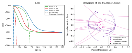
We numerically illustrate the importance of constraints in SSL. We consider a contrastive setting (loss in (1)) for the half moon dataset (Pedregosa et al. 2011), where is an independent sample from the dataset and where . Let us now compare the dynamics of (no constraints) and , the scaling loss that corresponds to orthogonality constraints, and present the results in Figure 1. We observe that under orthogonal constraints, independent of the initialization the function converges to fixed points (which we theoretically show in Theorem 3). On the other hand the dynamics for unconstrained loss diverge.
Non-Linear SSL Models are Almost Linear
While the above discussion pertains to only linear models, we now show that the network, with nonlinear activation and orthognality constraints,
is almost linear. For this discussion, we explicitly mention the time dependence as a subscript . We begin by arguing theoretically that in the infinite width limit at initialization there is very little difference between the output of the non-linear machine and that of its linear counterpart .
Theorem 1 (Comparison of Linear and Non-linear Network).
Recall that provides the output of the machine at time and therefore consider the linear and non-linear setting at initialization as
| (6) | |||||
Let be an activation function, such that , , and 333This last assumption can also be weakened to say that is continuous at . See the proof of the theorem for details. Then at initialization as uniformly random orthogonal matrices
where is an universal constant , is the feature dimension and the width of the hidden layer.
We furthermore conjecture that the same behaviour holds during evolution.
Conjecture 1 (Evolution of Non-linear Networks).
Numerical justification of the above conjecture is presented in the following section.
Numerical Evaluation.
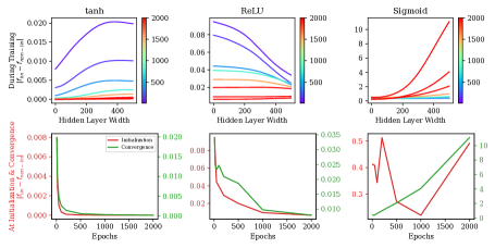
We now illustrate the findings of of Theorem 1 and Conjecture 1 numerically. For evaluation we use the following experimental setup: We train a network with contrastive loss as defined in (1) using gradient descent with learning rate for epochs and hidden layer size from to . We consider the following three loss functions: (1) sigmoid, (2) ReLU and (3) tanh. The results are shown in Figure 2 where the plot shows the average over initializations. We note that tanh fulfills the conditions on and we see that with increasing layer size the difference between linear and non-linear goes to zero. While ReLU only fulfills the overall picture still is consistent with tanh but with slower convergence. Finally the results on sigmoid (which has a linear drift consistent with its value at ) indicate that the conditions on are necessary as we observe the opposite picture: with increased layer width the difference between linear and non-linear increases.
Learning Dynamics of Linear SSL Models
Having showed that the non-linear dynamics are close to the linear ones we now analyze the linear dynamics. We do so by first showing that the two SSL settings discussed in the introduction can be phrased as a more general trace minimization problem. From there we derive the learning dynamics and discuss the evolution of the differential equation. Furthermore we numerically evaluate the theoretical results and show that the dynamics coincide with learning the general loss function under gradient decent.
We can define a simple linear embedding function as: where the feature dimension is for data points. The hidden layer dimension is and embedding dimension , such that the weights are given by . Therefore we can write our loss function as
with
| (7) |
Furthermore (1) can easily be extended to the positive and negative sample setting where we then obtain In addition we can also frame the previously considered non-contrastive model in (2) in the simple linear setting by considering the general loss function with We can now consider the learning dynamics of models, that minimize objects of the form
Definition 1 (General Loss Function).
Consider the following loss function
| (8) | ||||
where and are the trainable weight matrices. is a symmetric, data dependent matrix.
With the general optimization problem set up we can analyze (8) by deriving the dynamics under orthogonality constraints on the weights, which constitutes gradient descent on the Grassmannian manifold. While orthogonality constraints are easy to initialize the main mathematical complexity arises from ensuring that the constraint is preserved over time. Following (Lai, Lim, and Ye 2020), we do so by ensuring that the gradients lie in the tangent bundle of orthogonal matrices.
Theoretical Analysis
In the following we present the dynamics in Theorem 2, followed by the analysis of the evolution of the dynamics in Theorem 3.
Theorem 2 (Learning Dynamics in the Linear Setting).
Let us recall the the general linear trace minimization problem stated in (8):
where and are the trainable weight matrices and a symmetric, data dependent matrices, such that with . Then with , where represents the machine function i.e. , the learning dynamics of , the machine outputs are given by
| (9) |
Similar differential equations to (9) have been analysed in (Yan, Helmke, and Moore 1994) and (Fukumizu 1998). The typical way to find stable solutions to such equations involve converting it to a differential equation on . This gives us a matrix riccati type equation. For brevity’s sake we write below a complete solution when .
Evolution of the differential equation. While the above differential equation doesn’t seem to have a simple closed form, a few critical observations can still be made about it - particularly about what this differential equation converges to. As observed in Figure 3 (right), independent of initialisation we converge to either of two points. In the following we formalise this observation.
Theorem 3 (Evolution of learning dynamics in (9) for ).
Let then our update rule simplifies to
| (10) |
We can distinguish two cases:
-
•
Assume all the eigenvalues of are strictly positive then converges to .
-
•
Assume there is at least one negative eigenvalue of , then becomes the smallest eigenvector, .
The requirement of negative eigenvalues of for a non-trivial convergence might be surprising however we can observe this when considering in expectation. Let us assume is constructed by (7) and note that While this already gives a heuristic of what is going on, for some more precise mathematical calculations, we can specialise to the situation where is given by an independent sample and is given by adding a noise value sampled from , i.e. . Then
Thus is in fact negative definite.
New Datapoint. While the above dynamics provide the setting during training we can furthermore investigate what happens if we input a new datapoint or a testpoint to the machine. Because is a linear function and because is a basis this is quite trivial. So if is a new point, let be the co-ordinates of , i.e. or . Then
Numerical Evaluation
We can now further illustrate the above derived theoretical results empirically.
Leaning dynamics (Theorem 2) and new Datapoint. We can now illustrate that the derived dynamics in (9) do indeed behave similar to learning (8) using gradient decent updates. To analyze the learning dynamics we consider the gradient decent update of (8):
| (11) |
where are the weights at time step and is the learning rate as a reference. Practically the constraints in (8) are enforced by projecting the weights back onto and after each gradient step. Secondly we consider a discretized version of (9)
| (12) |
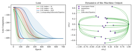
where is the machine outputs at time step . We now illustrate the comparison through in Figure 3 where we consider different width of the network and . We can firstly observe on the left, that the loss function of the trained network and the dynamics and observe while the decay is slightly slower in the dynamics setting both converge to the same final loss value. Secondly we can compare the function outputs during training in Figure 3 (right): We initialize the NN randomly and use this initial machine output as . We observe that during the evolution using (11) & (12) for a given initialization the are stay close to each other and converge to the same final outputs.
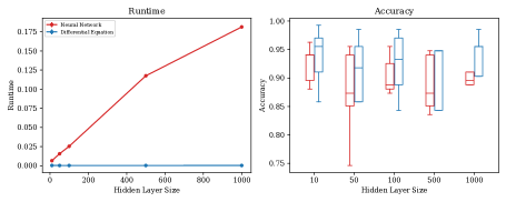
Runtime and downstram task. Before going into the illustration of the dynamics we furthermore note that an update step using (12) is significantly faster then a SGD step using (11). For this illustration we now consider two classes with 200 datapoints each from the MNIST dataset (Deng 2012). This is illustrated in Figure 4 (left) where we compare the runtime over different layer width (of which (12) is independent of). Expectantly (11) scales linearly with and overall (12) has a shorter runtime per timestep. While throughout the paper we focus on the obtained embeddings we can furthermore consider the performance of downstream tasks on top of the embeddings. We illustrate this in the setting above where we apply a linear SVM on top of the embeddings. The results are shown in Figure 4 (right) where we observe that overall the performance of the downstream task for both the SGD optimization and the differential equation coincide.
Conclusion
The study of learning dynamics of (infinite-width) neural networks has led to important results for the supervised setting. However, there is little understanding of SSL dynamics. Our initial steps towards analysing SSL dynamics encounters a hurdle: standard SSL training has drastic dimension collapse (Proposition 1), unless there are suitable constraints. We consider a general formulation of linear SSL under orthogonality constraints (8), and derive its learning dynamics (Theorem 2). We also show that the derived dynamics can approximate the SSL dynamics using wide neural networks (Theorem 1) under some conditions on activation . We not only provide a framework for analysis of SSL dynamics, but also shows how the analysis can critically differ from the supervised setting. As we numerically demonstrate, our derived dynamics can be used an efficient computational tool to approximate SSL models. In particular, the equivalence in Proposition 3 ensures that the orthogonality constraints can be equivalently imposed using a scaled loss, which is easy to implement in practice. We conclude with a limitation and open problem. Our analysis relies on a linear approximation of wide networks, but more precise characterisation in terms of kernel approximation (Jacot, Gabriel, and Hongler 2018; Liu, Zhu, and Belkin 2020) may be possible, which can better explain the dynamics of deep SSL models. However, integrating orthogonality or operator norm constraints in the NTK regime remains an open question.
Acknowledgments
This work has been supported by the German Research Foundation through the SPP-2298 (project GH-257/2-1), and also jointly with French National Research Agency through the DFG-ANR PRCI ASCAI.
References
- Alemohammad et al. (2021) Alemohammad, S.; Wang, Z.; Balestriero, R.; and Baraniuk, R. G. 2021. The Recurrent Neural Tangent Kernel. In International Conference on Learning Representations.
- Arora et al. (2019a) Arora, S.; Du, S. S.; Hu, W.; Li, Z.; Salakhutdinov, R.; and Wang, R. 2019a. On Exact Computation with an Infinitely Wide Neural Net. In International Conference on Neural Information Processing Systems.
- Arora et al. (2019b) Arora, S.; Khandeparkar, H.; Khodak, M.; Plevrakis, O.; and Saunshi, N. 2019b. A Theoretical Analysis of Contrastive Unsupervised Representation Learning. In International Conference on Machine Learning.
- Balestriero and LeCun (2022) Balestriero, R.; and LeCun, Y. 2022. Contrastive and Non-Contrastive Self-Supervised Learning Recover Global and Local Spectral Embedding Methods. In Advances in Neural Information Processing Systems.
- Bansal, Kaplun, and Barak (2021) Bansal, Y.; Kaplun, G.; and Barak, B. 2021. For self-supervised learning, Rationality implies generalization, provably. In 9th International Conference on Learning Representations.
- Bao, Nagano, and Nozawa (2022) Bao, H.; Nagano, Y.; and Nozawa, K. 2022. On the Surrogate Gap between Contrastive and Supervised Losses. In International Conference on Machine Learning.
- Bardes, Ponce, and LeCun (2021) Bardes, A.; Ponce, J.; and LeCun, Y. 2021. Vicreg: Variance-invariance-covariance regularization for self-supervised learning. arXiv preprint arXiv:2105.04906.
- Bromley et al. (1993) Bromley, J.; Guyon, I.; LeCun, Y.; Säckinger, E.; and Shah, R. 1993. Signature verification using a” siamese” time delay neural network. Advances in neural information processing systems.
- Cabannes et al. (2023) Cabannes, V.; Kiani, B. T.; Balestriero, R.; LeCun, Y.; and Bietti, A. 2023. The SSL Interplay: Augmentations, Inductive Bias, and Generalization. CoRR, abs/2302.02774.
- Caron et al. (2020) Caron, M.; Misra, I.; Mairal, J.; Goyal, P.; Bojanowski, P.; and Joulin, A. 2020. Unsupervised learning of visual features by contrasting cluster assignments. Advances in neural information processing systems.
- Caron et al. (2021) Caron, M.; Touvron, H.; Misra, I.; Jégou, H.; Mairal, J.; Bojanowski, P.; and Joulin, A. 2021. Emerging properties in self-supervised vision transformers. In Proceedings of the IEEE/CVF International Conference on Computer Vision.
- Chen et al. (2022) Chen, C.; Zhang, J.; Xu, Y.; Chen, L.; Duan, J.; Chen, Y.; Tran, S.; Zeng, B.; and Chilimbi, T. 2022. Why do We Need Large Batchsizes in Contrastive Learning? A Gradient-Bias Perspective. In Advances in Neural Information Processing Systems.
- Chen et al. (2020) Chen, T.; Kornblith, S.; Norouzi, M.; and Hinton, G. 2020. A simple framework for contrastive learning of visual representations. In International conference on machine learning. PMLR.
- Chen and He (2021) Chen, X.; and He, K. 2021. Exploring Simple Siamese Representation Learning. In IEEE Conference on Computer Vision and Pattern Recognition.
- Chen et al. (2021) Chen, Y.; Huang, W.; Nguyen, L. M.; and Weng, T. 2021. On the Equivalence between Neural Network and Support Vector Machine. In Advances in Neural Information Processing Systems 34.
- Deng (2012) Deng, L. 2012. The mnist database of handwritten digit images for machine learning research. IEEE Signal Processing Magazine.
- Devlin et al. (2019) Devlin, J.; Chang, M.; Lee, K.; and Toutanova, K. 2019. BERT: Pre-training of Deep Bidirectional Transformers for Language Understanding. In Proceedings of the 2019 Conference of the North American Chapter of the Association for Computational Linguistics: Human Language Technologies,.
- Du et al. (2019) Du, S. S.; Hou, K.; Salakhutdinov, R. R.; Poczos, B.; Wang, R.; and Xu, K. 2019. Graph Neural Tangent Kernel: Fusing Graph Neural Networks with Graph Kernels. In Advances in Neural Information Processing Systems, volume 32.
- Edelman, Arias, and Smith (1998) Edelman, A.; Arias, T. A.; and Smith, S. T. 1998. The geometry of algorithms with orthogonality constraints. SIAM journal on Matrix Analysis and Applications.
- Ermolov et al. (2021) Ermolov, A.; Siarohin, A.; Sangineto, E.; and Sebe, N. 2021. Whitening for self-supervised representation learning. In International Conference on Machine Learning.
- Fernando et al. (2017) Fernando, B.; Bilen, H.; Gavves, E.; and Gould, S. 2017. Self-supervised video representation learning with odd-one-out networks. In IEEE conference on computer vision and pattern recognition.
- Fukumizu (1998) Fukumizu, K. 1998. Dynamics of batch learning in multilayer neural networks. In ICANN 98: Proceedings of the 8th International Conference on Artificial Neural Networks. Springer.
- Ge et al. (2023) Ge, J.; Tang, S.; Fan, J.; and Jin, C. 2023. On the Provable Advantage of Unsupervised Pretraining. arXiv preprint, abs/2303.01566.
- Gidaris, Singh, and Komodakis (2018) Gidaris, S.; Singh, P.; and Komodakis, N. 2018. Unsupervised representation learning by predicting image rotations. arXiv preprint arXiv:1803.07728.
- Grill et al. (2020) Grill, J.; Strub, F.; Altché, F.; Tallec, C.; Richemond, P. H.; Buchatskaya, E.; Doersch, C.; Pires, B. Á.; Guo, Z.; Azar, M. G.; Piot, B.; Kavukcuoglu, K.; Munos, R.; and Valko, M. 2020. Bootstrap Your Own Latent - A New Approach to Self-Supervised Learning. In Advances in Neural Information Processing Systems.
- Han, Ye, and Zhan (2023) Han, L.; Ye, H.; and Zhan, D. 2023. Augmentation Component Analysis: Modeling Similarity via the Augmentation Overlaps. In The Eleventh International Conference on Learning Representations.
- HaoChen et al. (2021) HaoChen, J. Z.; Wei, C.; Gaidon, A.; and Ma, T. 2021. Provable Guarantees for Self-Supervised Deep Learning with Spectral Contrastive Loss. In Advances in neural information processing systems.
- Heckel and Yilmaz (2021) Heckel, R.; and Yilmaz, F. F. 2021. Early Stopping in Deep Networks: Double Descent and How to Eliminate it. In International Conference on Learning Representations.
- Jacot, Gabriel, and Hongler (2018) Jacot, A.; Gabriel, F.; and Hongler, C. 2018. Neural Tangent Kernel: Convergence and Generalization in Neural Networks. In International Conference on Neural Information Processing Systems.
- Jing and Tian (2019) Jing, L.; and Tian, Y. 2019. Self-Supervised Visual Feature Learning With Deep Neural Networks: A Survey. IEEE Transactions on Pattern Analysis and Machine Intelligence.
- Jing et al. (2022) Jing, L.; Vincent, P.; LeCun, Y.; and Tian, Y. 2022. Understanding Dimensional Collapse in Contrastive Self-supervised Learning. In The Tenth International Conference on Learning Representations.
- Johnson, Hanchi, and Maddison (2023) Johnson, D. D.; Hanchi, A. E.; and Maddison, C. J. 2023. Contrastive Learning Can Find An Optimal Basis For Approximately View-Invariant Functions. In International Conference on Learning Representations.
- Kanazawa, Jacobs, and Chandraker (2016) Kanazawa, A.; Jacobs, D. W.; and Chandraker, M. 2016. Warpnet: Weakly supervised matching for single-view reconstruction. In IEEE Conference on Computer Vision and Pattern Recognition.
- Kiani et al. (2022) Kiani, B. T.; Balestriero, R.; Chen, Y.; Lloyd, S.; and LeCun, Y. 2022. Joint Embedding Self-Supervised Learning in the Kernel Regime. CoRR, abs/2209.14884.
- Kunin et al. (2019) Kunin, D.; Bloom, J.; Goeva, A.; and Seed, C. 2019. Loss Landscapes of Regularized Linear Autoencoders. In Proceedings of the 36th International Conference on Machine Learning.
- Lai, Lim, and Ye (2020) Lai, Z.; Lim, L.-H.; and Ye, K. 2020. Simpler Grassmannian optimization.
- Lee et al. (2021) Lee, J. D.; Lei, Q.; Saunshi, N.; and Zhuo, J. 2021. Predicting What You Already Know Helps: Provable Self-Supervised Learning. In Advances in Neural Information Processing Systems.
- Li et al. (2021) Li, J.; Nguyen, T. V.; Hegde, C.; and Wong, R. K. W. 2021. Implicit Sparse Regularization: The Impact of Depth and Early Stopping. In Advances in Neural Information Processing Systems.
- Liu, Zhu, and Belkin (2020) Liu, C.; Zhu, L.; and Belkin, M. 2020. On the linearity of large non-linear models: when and why the tangent kernel is constant. In Advances in Neural Information Processing Systems 33.
- Liu et al. (2023) Liu, Z.; Lubana, E. S.; Ueda, M.; and Tanaka, H. 2023. What shapes the loss landscape of self supervised learning? In International Conference on Learning Representations.
- Luo et al. (2019) Luo, P.; Wang, X.; Shao, W.; and Peng, Z. 2019. Towards Understanding Regularization in Batch Normalization. In International Conference on Learning Representations.
- Misra and Maaten (2020) Misra, I.; and Maaten, L. v. d. 2020. Self-supervised learning of pretext-invariant representations. In Proceedings of the IEEE/CVF Conference on Computer Vision and Pattern Recognition.
- Mohamed et al. (2022) Mohamed, A.-R.; yi Lee, H.; Borgholt, L.; Havtorn, J. D.; Edin, J.; Igel, C.; Kirchhoff, K.; Li, S.-W.; Livescu, K.; Maaløe, L.; Sainath, T. N.; and Watanabe, S. 2022. Self-supervised speech representation learning: A review. IEEE JSTSP Special Issue on Self-Supervised Learning for Speech and Audio Processing.
- Neyshabur et al. (2017) Neyshabur, B.; Bhojanapalli, S.; McAllester, D.; and Srebro, N. 2017. Exploring Generalization in Deep Learning. In Advances in Neural Information Processing Systems.
- Nguyen, Wong, and Hegde (2021) Nguyen, T. V.; Wong, R. K. W.; and Hegde, C. 2021. Benefits of Jointly Training Autoencoders: An Improved Neural Tangent Kernel Analysis. IEEE Transactions on Information Theory.
- Novotny et al. (2018) Novotny, D.; Albanie, S.; Larlus, D.; and Vedaldi, A. 2018. Self-supervised learning of geometrically stable features through probabilistic introspection. In IEEE Conference on Computer Vision and Pattern Recognition.
- Pedregosa et al. (2011) Pedregosa, F.; Varoquaux, G.; Gramfort, A.; Michel, V.; Thirion, B.; Grisel, O.; Blondel, M.; Prettenhofer, P.; Weiss, R.; Dubourg, V.; Vanderplas, J.; Passos, A.; Cournapeau, D.; Brucher, M.; Perrot, M.; and Duchesnay, E. 2011. Scikit-learn: Machine Learning in Python. Journal of Machine Learning Research.
- Pretorius, Kroon, and Kamper (2018) Pretorius, A.; Kroon, S.; and Kamper, H. 2018. Learning Dynamics of Linear Denoising Autoencoders. In International Conference on Machine Learning.
- Sabanayagam, Esser, and Ghoshdastidar (2022) Sabanayagam, M.; Esser, P.; and Ghoshdastidar, D. 2022. Representation Power of Graph Convolutions : Neural Tangent Kernel Analysis.
- Saunshi, Malladi, and Arora (2021) Saunshi, N.; Malladi, S.; and Arora, S. 2021. A Mathematical Exploration of Why Language Models Help Solve Downstream Tasks. In International Conference on Learning Representations.
- Saxe, McClelland, and Ganguli (2014) Saxe, A. M.; McClelland, J. L.; and Ganguli, S. 2014. Exact solutions to the nonlinear dynamics of learning in deep linear neural networks. In International Conference on Learning Representations.
- Sermanet et al. (2018) Sermanet, P.; Lynch, C.; Chebotar, Y.; Hsu, J.; Jang, E.; Schaal, S.; Levine, S.; and Brain. 2018. Time-contrastive networks: Self-supervised learning from video. In IEEE international conference on robotics and automation.
- Shah et al. (2022) Shah, A.; Sra, S.; Chellappa, R.; and Cherian, A. 2022. Max-Margin Contrastive Learning. In AAAI Conference on Artificial Intelligence.
- Soudry et al. (2018) Soudry, D.; Hoffer, E.; Nacson, M. S.; Gunasekar, S.; and Srebro, N. 2018. The Implicit Bias of Gradient Descent on Separable Data. Journal of Machine Learning Research.
- Steffen et al. (2019) Steffen, S.; Baevski, A.; Collobert, R.; and Auli, M. 2019. wav2vec: Unsupervised Pre-training for Speech Recognition.
- Tian (2022) Tian, Y. 2022. Understanding Deep Contrastive Learning via Coordinate-wise Optimization. In Advances in Neural Information Processing Systems.
- Tosh, Krishnamurthy, and Hsu (2021) Tosh, C.; Krishnamurthy, A.; and Hsu, D. 2021. Contrastive learning, multi-view redundancy, and linear models. In Algorithmic Learning Theory, Proceedings of Machine Learning Research.
- van den Oord, Li, and Vinyals (2018) van den Oord, A.; Li, Y.; and Vinyals, O. 2018. Representation Learning with Contrastive Predictive Coding. CoRR, abs/1807.03748.
- Wei, Xie, and Ma (2021) Wei, C.; Xie, S. M.; and Ma, T. 2021. Why Do Pretrained Language Models Help in Downstream Tasks? An Analysis of Head and Prompt Tuning. In Advances in Neural Information Processing Systems.
- Yan, Helmke, and Moore (1994) Yan, W.-Y.; Helmke, U.; and Moore, J. 1994. Global analysis of Oja’s flow for neural networks. IEEE Transactions on Neural Networks.
- Zhai et al. (2023) Zhai, R.; Liu, B.; Risteski, A.; Kolter, Z.; and Ravikumar, P. 2023. Understanding Augmentation-based Self-Supervised Representation Learning via RKHS Approximation. CoRR, abs/2306.00788.
- Zhang et al. (2017) Zhang, C.; Bengio, S.; Hardt, M.; Recht, B.; and Vinyals, O. 2017. Understanding deep learning requires rethinking generalization. In International Conference on Learning Representations.
- Zhuo et al. (2023) Zhuo, Z.; Wang, Y.; Ma, J.; and Wang, Y. 2023. Towards a Unified Theoretical Understanding of Non-contrastive Learning via Rank Differential Mechanism. In The Eleventh International Conference on Learning Representations.
Appendix
In the supplementary material we provide the following additional proofs and results
Proof of Lemma1
Proof.
Let the collumns of be denoted by . Then we note that each component of , is given by . Thus if , has no dependence with i.e. . Thus we get that when ,
We can now use (Liu, Zhu, and Belkin 2020) (for instance its Lemma 1) which basically concludes that no training happens at the penultimate or prior layers. In limit all positive gradients arise only from the final layer. As such
By the same token, for ,
Finally again using the fact that does not change in training and that is initialized from a normalized gaussian , when is the identity map, it is well known that the above converges to (as there ) and otherwise to a deterministic kernel (see e.g. (Liu, Zhu, and Belkin 2020), (Arora et al. 2019b)). ∎
Proof of Proposition 1
Proof.
For simplicity of the proof we begin by reformulating the loss function in both contrastive and noncontrastive setting to a more general form. In particular it is trivial to check that we can generalize by writing
where denotes the collection of all the relevant data (i.e. , as well as and where applicable), and in the contrastive setting (equation 1) while in the non-contrastive setting (equation 2.)
Then decompose
Note then that Thus the optimization target,
Thus when the Frobenius norm is restricted (i.e. bounded between and ), if has atleast one negative eigenvalue the loss is minimized when is the eigenvector corresponding to the most negative eigenvalue of with , with no other non-zero singular value. On the other hand if has no negative eigenvalue then the loss is minimized when ∎
Proof of Proposition 3
Proof.
We begin by quickly observing that This is simply done by defining for . Then we have
Using the fact that at least one eigenvalue of is strictly negative (this rules out the case that the optimal is achieved when as that would have prevented division by norm) then we can quickly get that
For , we begin by observing that by submultiplicativity of norm, any such that and automatically falls is the optimization space given by thus giving one direction of the optimization equivalence for free. For the other side we note that given any such that , we can construct such that and . This follows from considering the singular values decomposition of , getting . As the norm of the product is smaller than , all the entries of the singular value matrix are less than . Thus depending upon which among or is larger we consider either the matrices and or the matrices and to be our candidate and respectively. To complete we will simply have to add zero rows to our choice i.e. say and to match the dimensions (i.e. to get a matrix from a one).
Finally for we begin by defining . Then the optimization problem in (3) becomes,
We then prove that we are done if we can prove the claim at optimal of (3) (i.e. the above optimization problem) all the eigenvalues of are or . Given this claim the singular value decomposition of becomes only , where if , is a matrix and a matrix. Additionally by property of SVD, the collumns of and are orthonormal. Finally as
we can add a bunch of zero rows to and to get our and matrices which will be our corresponding and .
It remains to prove that is minimized when all the eigenvalues of are or . To do this simply decompose
where is the set of orthonormal eigenvectors of corresponding to non-zero eigenvalues of (or alternatively non-zero singular values of ) Then
Thus if has many strictly negative eigenvalues with corresponding eigenvectors and is positive the above quantity is minimized by choosing as many of these as possible i.e. and setting the corresponding to be while every setting all other eigen-values to .
We then also note by consequence of the above proof that we avoid dimension collapse when possible i.e. when has multiple strictly negative eigenvalues (which is what one should expect if the data is not one dimensional as ) ∎
Proof of Theorem 1
Proof.
Let us start by defining some properties for the non-linearity: Assume the non-linear function is continuously twice differentiable near and has no bias i.e. Then via scaling we can assume WLOG that . As , we get that 444We can actually also use the weaker assumption that is continuous at . Thus there is some bounded (compact) set containing and a constant such that ,
| (13) |
Recall that the mapping of the first weight matrix is given by under the constraint that . Under uniformly random initialization by Lemma 2 (see proof below) then with probability asymptotically going to we have that
Thus the norm of each row of we get with a.w.h.p. :
From there we can now write the value of each node in the layer using Cauchy-Schwarz inequality as
| (14) |
We now apply the non-linearity to this quantity and denote the output of the first layer after the non-linearity as
Define the vector , where
Then we have for large enough555Note that for the weaker assumption we can still use equation 13. This is because by equation 14,w.h.p. goes to and thus in limit:
| by equation 13 | ||||
| by equation 14 | ||||
where is the universal constant Combining this with the second layer we get the difference of the outputs of the two networks as
| as | ||||
∎
Lemma 2.
Given any , Let be a uniformly random semi-orthonormal matrix. I.e. is the first columns of an uniformly random orthonormal matrix. Then there are constants and a sequence converging to as goes to infinity such that ,
Proof.
We note that it is enough to prove the claim when , i.e. is uniformly random orthonormal matrix. Then as our distribution is uniform, the density at any particular is same as the density at any where is some other fixed orthogonal matrix. Thus if is the first column of , the marginal distribution of has the property that its density at any is same as that of for any orthogonal matrix . In other words the marginal distribution for any column of is simply that of the uniform unit sphere.
Consider then the following random variable which has the same distribution as that of a fixed column of i.e. uniform unit -sphere. Let be iid random variables from . Then we know that . From the rotational symmetry property of standard gaussian then we have that is distributed as an uniform sample from the unit sphere in dimensions. By union bound then, we have
As each is iid normal, is iid Chi-square with , thus by Chernoff there exists constants such that
Since and implies that , we get that
From the argument before that any ’th column of is distributed as . Using the above and another union bound then get us
We note that for any constants that as goes to infinity, both and goes to zero. The proof is then finished by choosing some appropriate constants . ∎
Proof of Theorem 2
Proof.
To simplify notation we are dropping the superscript from . The in the following proof is already presumed to be linear. For the same reason we are also dropping the symbol of time, , from even though all of them are indeed time dependent. Finally for any time dependent function , we denote by .
From (Edelman, Arias, and Smith 1998), we get that the derivative of a function restricted to a grassmanian is derived by left-multiplying to the ”free” or unrestricted derivative of . Using this and recalling that the loss in Eq. 8 is given by
we therefore can write and as
Thus we obtain
where we obtain the second equality by expanding the terms, taking advantage of and . Now setting as and using the fact that they are eigenvectors for and using gives us:
Let’s rewrite this in matrix notation. First define thus obtaining:
which concludes the proof. ∎
Proof of Theorem 3
Proof.
For instance first suppose that all the eigenvalues of are strictly positive and thus . Then
Observing now that because of orthonormality of our weight matrices, we get that the derivative of is always negative and thus converges to .
Now suppose on the other hand there is atleast one negative eigenvalue. WLOG let denote the eigenvector with the smallest eigenvalue (which is negative). Then
We now note that as is the smallest eigenvalue. Thus as is positive, the derivative of is always positive unless , which only happens at . In other words, eventually becomes the smallest eigenvector . ∎