Logarithmic Mathematical Morphology: theory and applications
Abstract
Classically, in Mathematical Morphology, an image (i.e., a grey-level function) is analysed by another image which is named the structuring element or the structuring function. This structuring function is moved over the image domain and summed to the image. However, in an image presenting lighting variations, the analysis by a structuring function should require that its amplitude varies according to the image intensity. Such a property is not verified in Mathematical Morphology for grey level functions, when the structuring function is summed to the image with the usual additive law. In order to address this issue, a new framework is defined with an additive law for which the amplitude of the structuring function varies according to the image amplitude. This additive law is chosen within the Logarithmic Image Processing framework and models the lighting variations with a physical cause such as a change of light intensity or a change of camera exposure-time. The new framework is named Logarithmic Mathematical Morphology (LMM) and allows the definition of operators which are robust to such lighting variations. In images with uniform lighting variations, those new LMM operators perform better than usual morphological operators. In eye-fundus images with non-uniform lighting variations, a LMM method for vessel segmentation is compared to three state-of-the-art approaches. Results show that the LMM approach has a better robustness to such variations than the three others.
Index Terms:
Mathematical morphology, lighting variations, order-statistic filters, intensity-variant structuring function, robustness to lighting variations, Asplund metric.1 Introduction
Mathematical Morphology (MM) was originally defined by Matheron [1] for sets and then extended to functions with real values by Serra [2], Sternberg [3, 4] and Maragos [5]. In this latter case, a function is analysed by another function named structuring element or structuring function. This extension includes grey level images whose values are within the bounded interval of the real space . For example, for 8 bit-digitised images, is equal to 256. Generally, structuring functions and morphological operators are invariant under horizontal translations (i.e. in space) and under vertical translations (i.e. in intensity) [6].
However, the application of MM to grey level images presents two limitations. (1) Firstly, albeit grey level images have bounded values, MM was defined for functions with values within the unbounded real space [7, 8]. Indeed, given an image and a structuring function both defined on the same domain and whose values are within the range , their sum does not lie within the interval . Practical solutions to this issue consist of using either (i) a structuring function whose supremum is equal to zero, (ii) or a flat structuring element whose values are equal to zero (iii) or to truncate the values of the resulting image to the maximal possible value, [7]. (2) Secondly, adding a structuring function to an image without taking into account the image intensity into the amplitude of the structuring function is not physically justified. As in human vision, the eye response to light intensity variations is known to be logarithmic [9, 10, 11, 12, 13], it follows that in images the contrast variations are also logarithmic and the darkest variations are more attenuated than the brightest ones [14, 15]. The amplitude of the structuring function must therefore depend on the image intensity, i.e. the grey value. Such a structuring function will be invariant under horizontal translation but not under vertical translation, i.e. in the intensity domain .
In parallel to the genesis of grey-level MM, Jourlin has developed the Logarithmic Image Processing (LIP) model which is adapted to human vision [9, 16, 17] and which allows to process images as a human eye would do. It is not only rigorously defined from a mathematical point of view, but it also possesses strong physical properties. In particular, the LIP-addition of two images results in an image (with bounded values within the interval ). It also allows to simulate the variations of light intensity or of camera exposure-time in images.
The aim of this paper is to address both previously listed limitations of the MM application to grey level images by presenting a new framework named Logarithmic Mathematical Morphology (LMM) that was recently introduced [18, 19, 20]. Such a framework allows to adjust the amplitude of the structuring function according to the image intensity thanks to the LIP-addition between the image and the structuring function. LMM extends the theory of MM for images and functions by introducing operations of Logarithmic Image Processing.
In this article and beyond the prior work, the theory of LMM will be detailed. New theoretical results will be added at both following levels. (1) A link will be established between LMM and the functional Asplund metric defined with the LIP-additive law . Such a metric is robust to lighting variations caused by a change of the light intensity or the camera exposure-time [17]. (2) New morphological operators with the same robustness to lighting variations will be introduced for non flat structuring functions. LMM will also be validated with experiments and compared to state-of the art methods.
2 Related work: detection operators robust to lighting variations
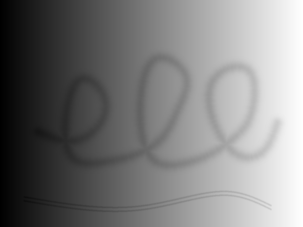
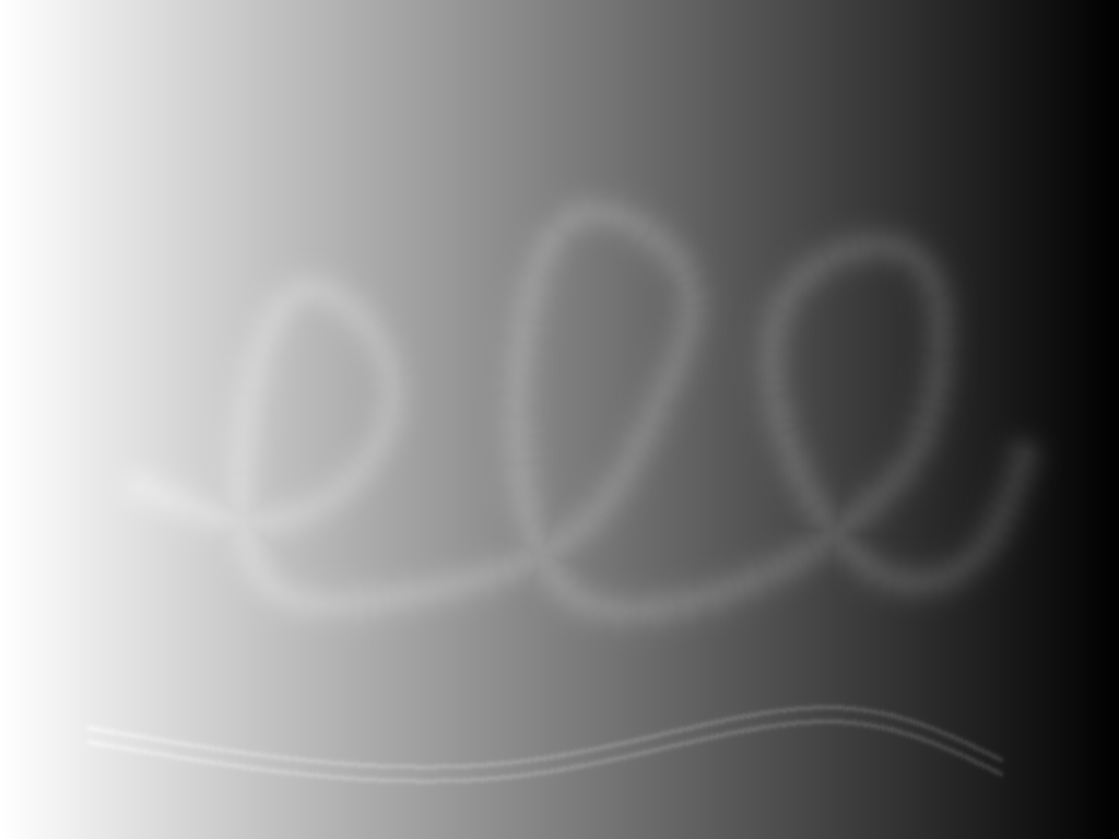
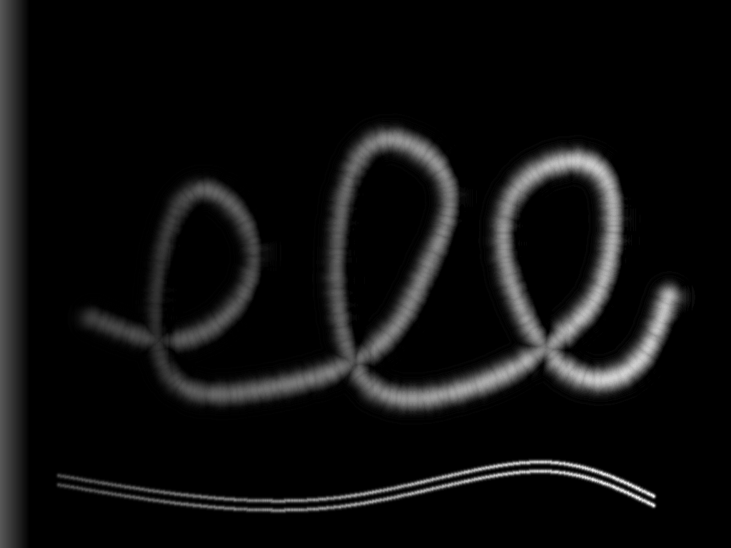
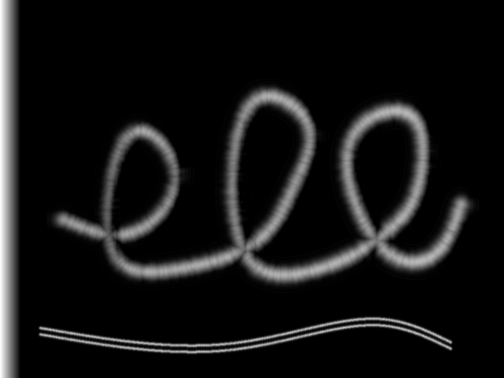
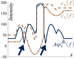
Previously in the literature, there has been some attempts to create operators theoretically robust to lighting changes. However, such operators generally do not take into account the physical causes of these lighting changes such as variations of light intensity or equivalently variations of camera exposure-time. In LMM, these causes are modelled by the LIP-additive law [17]. Figure1, shows an image composed of a spiral, a lighting drift and two confounding curves (Fig. 1a). In this example, the LMM operator better detects the spiral without the confounding curves (Fig. 1f) than the usual methods based on a top-hat (Fig. 1d) or a logarithmic top-hat (Fig. 1e).
Let be a function defined on a domain whose values are lying in . Let be a structuring function whose values are equal to outside a domain , , . In addition, if its values in are equal to zero, the structuring function is called a (flat) structuring element and it is represented by the upper-case letter .
2.1 Top-hat operators
Meyer [21, 2] created the top-hat operator to detect peaks in a function . It is equal to the difference between the function and its morphological opening by a flat structuring element , . The complementary operation for the detection of valleys is the bottom-hat defined as the difference between a morphological closing of the function and the function itself, . Both top-hats are invariant to artificial variations of intensity caused by the addition or the subtraction of any real constant to a function , and . However, they are not invariant to any lighting variation with a physical cause and modelled by a LIP-addition or a LIP-subtraction of a constant to an image . To address this issue, Jourlin et al. [22, 16] have introduced LIP top-hats where the LIP-difference replaces the usual difference “”. Zaharescu [23] proposed variants of LIP top-hats. However, all these top-hats are still defined with a flat structuring element. They constitute a particular case of the extended tops-hats that will be presented in this paper (in section 5.4).
2.2 Morphological gradients
Beucher [24] defined the morphological gradient as the difference between the dilation and the erosion of a function by a flat structuring element , . The so-called “morphological gradient” corresponds in fact to the norm of the usual gradient of a function [25]. In order to be the norm of a gradient, it must be defined with a flat structuring element. It is invariant to the addition or subtraction of any real constant to a function, . However, it is not invariant to a lighting variation with a physical cause and modelled by a LIP-addition or a LIP-subtraction of a constant to an image. Jourlin [22] addressed this issue by defining a LIP-morphological gradient where the LIP-difference replaces the usual difference “”,.
2.3 Scale Invariant Feature Transform (SIFT)
Lowe introduced the Scale Invariant Feature Transform to detect image features which are “partially invariant to change in illumination” [26]. In SIFT, salient points are first detected as some extrema of a function scale-space obtained by differences between Gaussian filtering of the image. A local image descriptor is then associated to each salient point. This image descriptor is based on an orientation histogram of the gradient of the Gaussian filtered image. As the gradient is computed by differences between image values, this makes it insensitive to illumination changes caused by the addition of a constant. The orientation is weighted by the norm of the gradient which is equal to the so-called “morphological gradient” and has therefore the same invariance. In addition, a normalisation between 0 and 1 of the orientation histograms makes the SIFT descriptor invariant to the multiplication of the image by a constant. However, such invariances do not have any physical causes.
2.4 Trees of connected components
Trees of connected components are based on level sets. An image level set is the set of these pixels whose values are greater or equal to a given threshold value. By increasing the threshold value, the connected components of a higher level set are included within the connected components of a lower level set. These inclusion relations can be represented by trees of connected components. Various types of trees can be built according to the inclusion relation between the level sets. One can cite e.g., the component-tree, also named max-tree [27], or the tree of shapes, also named inclusion tree [28]. Recent segmentation methods by trees of connected components have been presented in [29, 30]. Trees of connected components of a real function are theoretically invariant to intensity changes caused by applying to the function a continuous and increasing transformation. However, as the intensity of an image is quantised in discrete values in the range with a constant step, the lower intensities are poorly represented by these discrete values. For this reason, in low-lighted images, the connected components trees may present a limited robustness to lighting variations [31].
2.5 Intensity variant Mathematical Morphology
Heijmans [6] named t-operators the usual morphological operators for functions because of their invariance under horizontal translation (i.e. in space) and under vertical translation (i.e. in intensity). He also defined a class of morphological operators, the h-operators, which are invariant under horizontal translation but adaptive in the vertical domain (i.e. in intensity). Although the examples of h-operators given in [6] were mathematically well-defined for real functions, they were not physically justified. LMM operators form a particular case of h-operators which are in addition defined for functions with bounded values such as images and are physically justified.
3 Background
3.1 Mathematical Morphology
MM is defined on complete lattices [32, 7, 33]. A set on which a partial order relation is defined is called a complete lattice if every subset of has an infimum (i.e., a greatest lower bound), , and a supremum (i.e., a least upper bound), . In the case of MM for functions, the set of functions defined on a domain with values in is a complete lattice with the order . The infimum and the supremum are defined for any family by and , respectively. The least and greatest elements, and , are the constant functions equal to and , for all , respectively. Between any two complete lattices and , the fundamental morphological operations of erosion and dilation are defined as follows [34, 7, 33].
Definition 1.
A mapping or an operator is an erosion, if and only if (iff) it distributes over infima, that is , for any family . The operator is a dilation, iff it distributes over suprema, that is , for any .
The definitions of these mappings apply even to the empty subset of or because of the relations and [7]. We have therefore: and . Moreover, the pair forms an adjunction between and if for all , there is
| (1) |
In an adjunction , is an erosion and a dilation [7]. If one reverses the ordering of both lattices and , the dilation becomes an erosion and vice versa. The erosion and the dilation are called adjunct operators. The adjunction constitutes a bijection between the erosion and the dilation. For every dilation , there is a unique erosion such as is an adjunction and vice-versa. Moreover, if is an adjunction, then the combination is an opening on and the combination is a closing on [35]. Opening and closing are morphological filters defined as follows [1, 2, 35].
Definition 2.
An operator on the complete lattice is called an opening if is increasing (, if then ), anti-extensive (, ) and idempotent (). is a closing if it is increasing, extensive (, ) and idempotent.
In the lattice of real functions, let be a structuring function which is invariant under horizontal and vertical translations. The functional dilation and erosion are t-operators which are usually expressed [2] by:
| (2) | |||||
| (3) |
In the case of ambiguous expressions, the following conventions are used: when or , and when or [7]. The symbols and represent the extension to functions of Minkowski operations between sets [2]. Overviews of MM are available in [34, 36, 37, 38, 39] and some recent advances in the field can be found in [40, 41, 42, 43].
3.2 Logarithmic Image Processing
The LIP model is a mathematical framework which allows to process images in a way which is compatible with the human visual system [10, 17]. This makes it valid not only for images acquired with transmitted light but also with reflected light. The LIP model is based on the physical law of transmittances, , where the transmittance of the superimposition of two semitransparent objects generating the images and is equal to the point-wise product of their respective transmittances and . The transmittance at point is also related to the image grey value by the equation , where is the upper-bound of the grey value interval . Due to this relation, the LIP-scale is inverted compared to the usual grey scale (Figure 1b). This means that corresponds to the white extremity, when there is no obstacle between the light source and the camera, whereas corresponds to the black extremity when no light is passing. By replacing the transmittances and by their expressions in the transmittance law, the addition of two images and is deduced:
| (4) |
In transmitted light, the addition of two images corresponds to the superimposition of two semitransparent objects generating the images and . From (4), the LIP-multiplication of an image by a scalar is deduced, . It is equivalent to a variation of thickness or opacity of the object by a factor . If , the image becomes darker, whereas if it becomes brighter. The opposite function is then deduced:
| (5) |
One can notice that , where , is not an image as it takes negative values. It belongs to the set of real functions whose values are bounded by , . From a physical point of view, the negative values , where , are light intensifiers that can be used to compensate the attenuation of the semi-transparent object generating the image . Their superimposition with the image is equal to zero (i.e. the white intensity),. This is an important physical property that will be used in this paper. In particular, the LIP-addition of a negative constant will allow to compensate the light attenuation due to a variation of camera exposure-time or of light intensity [17]. From (5), the difference between two functions with bounded values and is deduced:
| (6) |
is an image iff . The space of functions whose values are bounded by , , is a real vector space and the space of images, , represents the positive cone of this vector space [16, 17]. and are both ordered by the usual order [16].
4 Logarithmic Mathematical Morphology
4.1 The new framework
LMM is defined in the lattice of functions with values in . The infimum and the supremum are defined for any family by and , respectively. The least and greatest elements, and , are the constant functions equal for all to and , respectively. The LIP-additive law and the LIP-negative law will allow to perform morphological transformations that are compatible with the human visual system. LMM is based on the adjunct operators of erosion and dilation which will be introduced as follows. Let be a function and a structuring function. Let and be both mappings defined by:
| (23) | |||||
| (40) |
In the case of ambiguous expressions, the following conventions will be used: when or , and when or . The following proposition111The proofs of the propositions 1, 2 and 3 are in the Supplementary Material. and definition hold.
Proposition 1.
The pair of mappings forms an adjunction, where is an erosion and is a dilation.
Definition 3.
is called a logarithmic-erosion and a logarithmic-dilation.
As forms an adjunction, an opening and a closing can be defined by combination of both operators of logarithmic-erosion and logarithmic-dilation (see. section 3.1). The operators and defined by
| (65) | |||||
| (90) |
are an opening and a closing (by adjunction), respectively.
Definition 4.
is called a logarithmic-opening and a logarithmic-closing.
Another useful property in MM is that the erosion of a function is equal to the dilation of its negative function, and vice versa. Such a property is the duality by negative function of both operators and, for LMM, it is established in proposition 2. The negative function of is equal to because we have [8].
Proposition 2.
Let be the reflected structuring function of , where , . The logarithmic-erosion and dilation are dual by their negative functions:
| (123) |
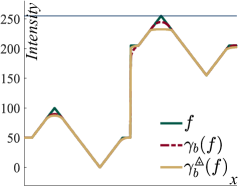
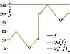
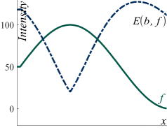
In the unidimensional image of Figure2, operators of functional MM are compared to those of LMM. A half-disk serves as structuring function (sf) . In LMM, the amplitude of the sf changes according to the image values because of the LIP-laws, or , used in (23) and (40). LMM operators are therefore h-operators which are only invariant under horizontal translation (see section 2.5). However in functional MM, the amplitude of the sf remains the same. This generates t-operators which are invariant under horizontal and vertical translations. Moreover, in Figure2b, the logarithmic-dilation of is always below the upper bound , whereas the functional dilation of may exceed this bound. Such a property is due to the LIP-addition law . In Figure2a, the negative values of the functional erosion have no physical justification, whereas those of the erosion correspond to light intensifiers. In Figure2c, the difference between the functional opening and the logarithmic-opening is greater for the grey-levels close to than for those close to zero. Indeed, in LMM, the amplitude of the sf is greater for higher image intensities than for lower intensities because of the non-linearity of the LIP laws and .The same observation exists between the functional closing and the logarithmic-closing (Figure2d).
4.2 Relation with functional Mathematical Morphology
LMM is defined in the lattice , whereas MM for functions is defined in the lattice . In order to relate LMM to functional MM, an isomorphism between both lattices is needed. This isomorphism and its inverse were both defined in [44] by and . With this isomorphism , the following proposition can be established.
Proposition 3.
Let be a function and a structuring function. The logarithmic-dilation and the logarithmic-erosion are related to the functional dilation , or , and erosion , or , respectively, by the equations:
| (132) | |||||
| (141) | |||||
where is equal to .
These relations facilitate the implementation of the LMM operators as those of usual MM already exist in numerous image analysis software.
4.3 Rank filters
Functional dilations and erosions are based on supremum and infimum operations. As supremum and infimum are very sensitive to noise such as speckle [35], they can be replaced by rank filters [36] also named order statistics filters [45], percentile filters or rank order filters. The filter of rank selects the smallest element of a set. It corresponds to the minimum represented by . Its dual, the maximum selects the greatest element of a set. In (3), a minimum filter can be defined by replacing the infimum by the the minimum . Similarly, in (2), a maximum filter can be defined with the maximum . If , the minimum filter is equal to the functional erosion and the maximum filter is equal to the functional dilation . In LMM, the minimum logarithmic filter and the maximum logarithmic filter can also be defined by using the minimum and the maximum in (40) and (23), respectively. The minimum and maximum logarithmic filters and are also related to the minimum and maximum filters and by replacing the erosions, and , and dilations, and , by their corresponding rank filters in (141) and (132).
5 Operators robust to lighting variations
Examples of operators robust to lighting changes caused by variations of the camera exposure-time or of the light intensity will be given. These lighting changes are modelled by the LIP-addition of a constant.
5.1 Map of LIP-additive Asplund distances
5.1.1 Link with LMM
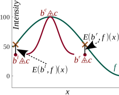
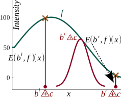
The functional Asplund metric with the LIP-additive law was defined by Jourlin [17]. Let and be two functions. One of them, e.g. , is chosen as a probing function and both following numbers are defined: and , where lies within the interval . and are the constants to be LIP-added to the probe such that it is in contact with the function from above or from below, respectively. The LIP-additive Asplund metric is defined by . Importantly, this metric is theoretically invariant under lighting changes modelled by a LIP-addition of a constant: , and [17].
The map of Asplund distances of a function of by a probe , where is a subset of , is the mapping . Such a mapping is obtained by computing the distance between the function and the probe for each point of the function domain . It is defined by , where is the restriction of to the neighbourhood centred on . The map of Asplund distances which was related to MM in [46, 47, 48], is equal to
| (158) |
where is the map of the least upper bounds (mlub) and is the map of the greatest lower bounds (mglb). The mlub is a dilation and the mglb is an erosion which are both equal, for all , to:
| (175) | |||||
| (192) | |||||
By comparing (175) with (23) and (192) with (40), there exists a strong link between the map of Asplund distances and LMM, as shown in the next proposition222The proof of proposition 4 is in Supplementary Material..
Proposition 4.
Let be a function and be a structuring function, where for all , , . The map of Asplund distances between the function and the structuring function is equal to:
| (233) |
For the mlub and the mglb of , and , we have:
| (250) | |||||
| (259) |
In the case of ambiguous expressions, the following conventions are used: when or , and when .
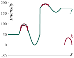
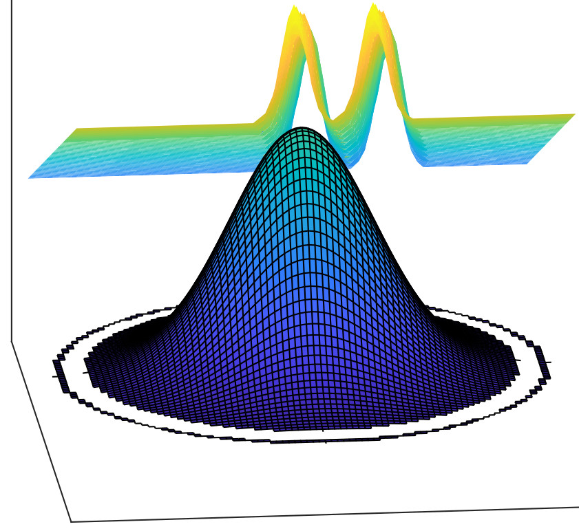
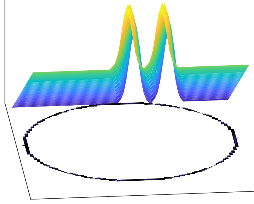
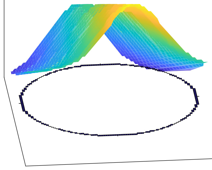
As illustrated in Figure3, the map of Asplund distances consists of a double probing of a function by the same probe from above and from below. The mlub and the mglb correspond to a dilation and an erosion of the image , respectively, by their respective structuring functions or (Figure3b). When the probe is similar to the image (according to the Asplund metric), the map of Asplund distances, , of the image presents a minimum. In Figure3b, both minima of the map of distances correspond to both bumps of the image (Figure3a).
5.1.2 Link with the LIP-morphological gradient
Let be a symmetric and constant structuring element which is defined for all , where , by and . In the case of a symmetric and constant structuring element , the map of LIP-additive Asplund distances is equal to the LIP-morphological gradient . For all , we have333The proofs of (268) and (285) are in Supplementary Material.:
| (268) |
is a flat structuring element with the same domain as the one of the constant structuring element .
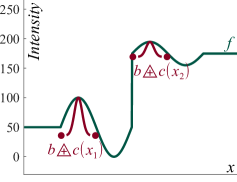
When the structuring function is non flat, the map of LIP-additive Asplund distances is an extension of the LIP-morphological gradient . However, contrary to the morphological gradient, the map of Asplund distances is no more the norm of a gradient. For example, let be a constant (i.e., a flat) zone of a function and let be the eroded flat zone by the domain of the structuring function . represents the binary erosion [2, 34]. In the eroded flat zone , the map of Asplund distances is equal to a constant, whereas a gradient and its norm should be equal to zero. We have, for all :
| (285) |
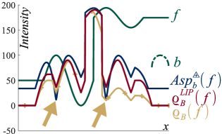
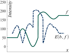
and are the supremum and the infimum, respectively, of the structuring function . In Figure4, the morphological gradient of the image and its LIP-morphological gradient , both with a flat structuring element , are compared to the map of Asplund distances with a structuring function . This structuring function has a bump shape which was designed to detect the bumps of the image . For both image bumps, the map of Asplund distances presents two deep minima with the same dynamic range, whereas the LIP-morphological gradient and the morphological gradient have two regional minima which have a lower dynamic range. In addition, the regional minima of the morphological gradient have not the same depth between each others. For the flat zones of the image , both gradients and are equal to zero, whereas the map of Asplund distances is equal to a positive constant defined by (285).
The map of LIP-additive Asplund distances is therefore the extension of the LIP-morphological gradient for non flat structuring functions. It gives to this gradient the properties of a metric which is robust to lighting variations. The LIP-morphological gradient is thereby a double probing of an image by a flat structuring element.
5.1.3 Map of Asplund distances with a tolerance to extrema
In the case of discrete images, a map of LIP-additive Asplund distances with a tolerance (to extrema) can be defined as in [47] and related to Mathematical Morphology as follows444The proof of proposition 5 is in Supplementary Material..
Proposition 5.
Let be a function defined on a discrete grid, e.g. . Let be a structuring function, where for all , , . Let be a percentage of points of to be discarded. The map of LIP-additive Asplund distances with a tolerance between the function and the structuring function is equal to:
| (326) |
The number of points to be suppressed, and , for the mlub and for the mglb are equal to and , respectively, where and is the cardinal of . For the mlub, , and the mglb of , , we have:
| (343) | |||||
| (352) |
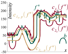
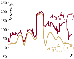
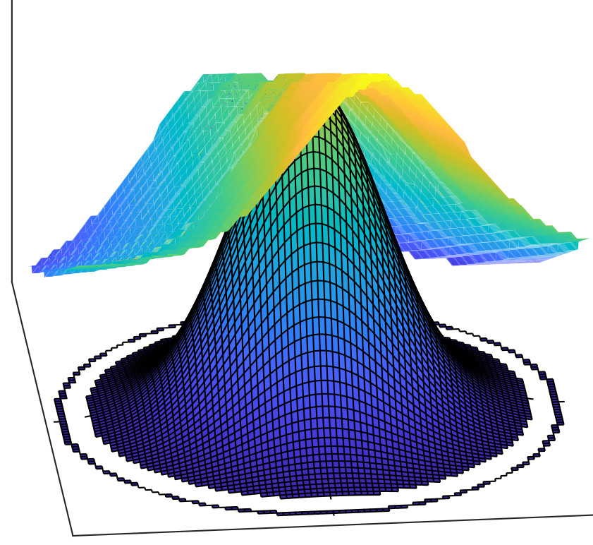
In Figure 5a, a Gaussian white noise is added to the image of Figure 3a in order to obtain a noised image . The mlub and the mglb of (without tolerance) are compared to the mlub and the mglb of with a tolerance . One can notice that these latter are less sensitive to the local extrema caused by peaks of noise. In Figure 5b, a similar observation can be made between the map of Asplund distances (without tolerance) and the map of Asplund distances of with tolerance . This latter map has a similar shape as the map of Asplund distances of the image without noise (Figure 3b).
5.2 A novel operator: the LIP-difference between LIP-erosions
In Figure6, a probe was designed to detect a bump (Figure6a) but not a transition (Figure6b) in a unidimensional image . The probe is composed of three elements: (i) the left point , (ii) the right point and (iii) a central bump with approximately the same dynamic range as the bump to be detected but with a smaller width. For each point of the domain , the probe is set in contact with the image from below by LIP-adding a constant . This latter one is equal to the value of the mglb, , which has been defined in (192). The LIP-difference is computed between the image and the left and right points, and , of the probe, , which is in contact with the image . The left and right detectors, and , are defined as follows:
| (385) | |||||
| (418) | |||||
In the event of a bump similar to the probe, the left and right detectors, and , will have close values (Figure 6a), whereas in the event of a transition, one of the detectors will have a value much higher than the other one (Figure 6b). Such a property allows to separate bumps (which are similar to the probe) from the transitions. The bump detector is therefore defined as the point-wise supremum between the left and right detectors:
| (419) |
As illustrated in Figure 6c, in the event of a bump, the detector presents a deep minimum, wheareas in the event of a transition, this minimum disappears. The left and right detectors are related to LMM by the following properties555The proofs of properties 1, 2 and 3 are in Supplementary Material..
Property 1.
The left and right detectors, and , are equal to LIP-differences between logarithmic-erosions:
| (444) | |||||
| (469) |
Property 2.
The left and right detectors, and , and the bump detector, , are insensitive to the LIP-addition (or the LIP-subtraction) of any constant to (or from) the image :
Figure 7a illustrates the application of the bump detector to a unidimensional image . The detector presents two minima of the same depth, one for each bump of the image. In the image , the bump amplitudes are related by the LIP-addition of a constant which models a change in the image intensity caused by a variation of the light intensity or of the exposure time of the camera. The bump detector is therefore robust to lighting variations modelled by the LIP-addition of a constant. Due to the LIP-addition of the image mglb, , to the probe , this latter has an amplitude which changes according to the image intensity (Figure 7b).
5.3 Other operators: LIP-differences between LIP-morphological operations
In the same way as in section 5.2, the LIP-difference between two operations of LMM can be robust to lighting variations. For example, Figure 1f illustrates the robustness to a lighting drift, of the operator defined by:
| (526) |
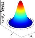
It is equal to the LIP-difference between two logarithmic openings and by two different probes and . is a Gaussian-shape probe surrounded by a ring (Figure 1c) and is a ring-shape probe. The operator possesses the following property.
Property 3.
The operator is insensitive to the LIP-addition of any constant to the function :
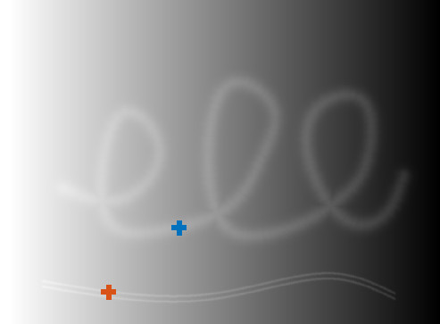
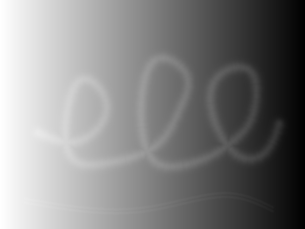

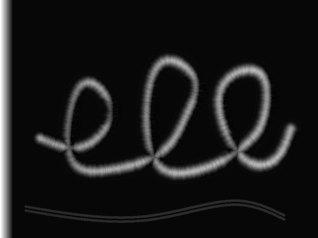
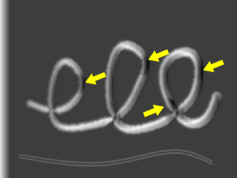
As the openings are performed by using the probe defined on a local domain , the operator is locally (and globally) insensitive to the addition of any constant in this domain . Such a local domain corresponds to a sliding window around any pixel of the image domain . In Figure 1a, the image presents a lighting drift caused by the LIP-addition of a linear function (i.e. a plane). As a plane (and several other lighting drifts) can be approximated by a piecewise constant function, the operator is robust to such a lighting drift. In addition, the Gaussian shape of the probe allows to detect the spiral without detecting both close curves. (i) Firstly, the width of the Gaussian at its top is larger than the width of each one of both curves, but it is smaller than the width of the spiral. When probing the image , as the probe is composed of a Gaussian and a ring, it cannot enter into the curves (Figure 8b), but it can enter into the spiral (Figure 8c). As a consequence, the logarithmic opening of by the Gaussian and ring probe almost completely removes both curves but it keeps the spiral (Figure 8d). (ii) Secondly, the ring probe is larger than the widths of the spiral and of both curves. This prevents it from entering into them (Figure 8e and 8f). The logarithmic opening of by the ring strongly attenuates the spiral and removes both curves (Figure 8g). In the resulting image (Figure 1f or 8h), the LMM operator extracts the spiral without the lighting drift and strongly attenuates the confounding curves. This image is obtained by the LIP-difference between both openings, (Figure 8d) and (Figure 8g), of the image by the probes and , respectively. However, the classical Mathematical Morphology operator defined as the difference between the openings and (Figure 8i), does not extract the spiral without keeping contrast changes caused by the lighting drift. A detection robust to lighting drifts – with a physical cause and modelled by the LIP-addition law – is therefore not possible by using classical MM operators, whereas it is possible by using LMM operators.
Other operators robust to lighting variations which are modelled by the LIP-additive law, can be defined as the LIP-difference between LMM operations, e.g.: the LIP-difference between logarithmic-closings or the LIP-difference between an image and its logarithmic-opening (see (553)).
5.4 Extensions of top-hat operators
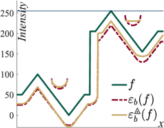
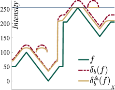
Let us focus on the difference, or residue, of an image by its opening or its logarithmic-opening . Both operators and are defined as follows:
| (528) | |||||
| (553) |
When is a flat structuring element denoted by , the operators and correspond to the top-hat operators and , respectively. These top-hat operators are presented in section 2.1. When is a non-flat structuring function, both operators and constitute extensions of the top-hat operators. The operator is named the extended top-hat and the operator the extended LIP-top-hat. However, only this latter operator possesses the following property666The proof of property 4 is in Supplementary Material..
Property 4.
The extended LIP-top-hat, , is insensitive to the LIP-addition of any constant to the function : .
6 Experiments and results
6.1 Robustness to lighting variations caused by changes in the exposure-time of a camera
6.1.1 Extended top-hats
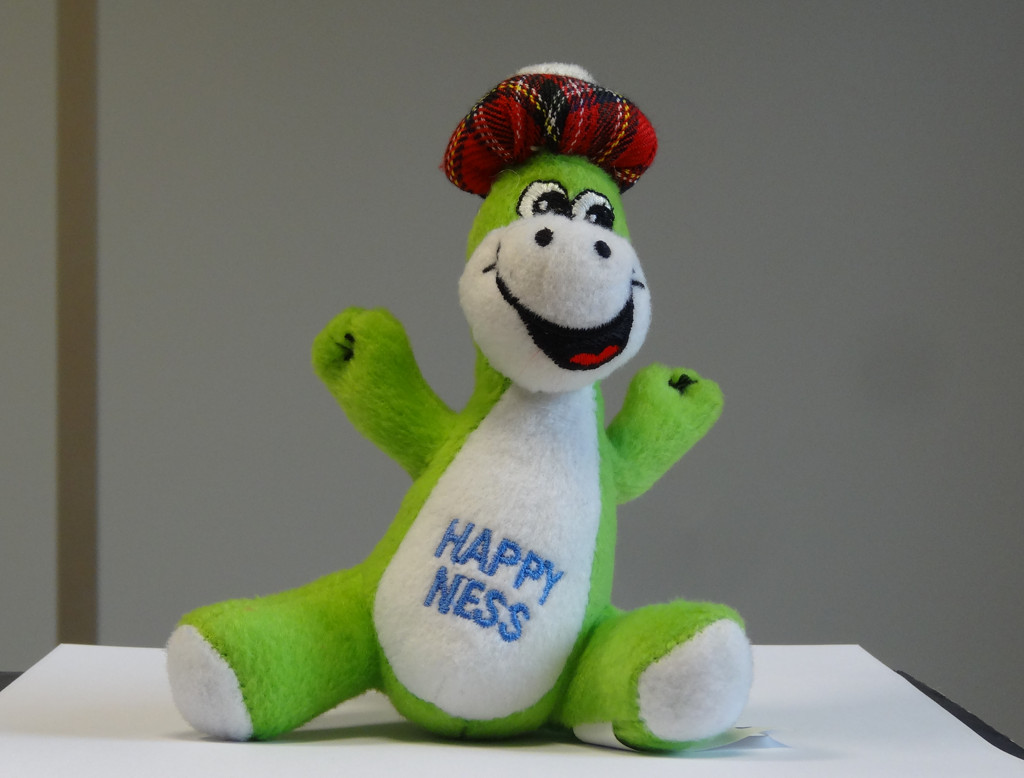
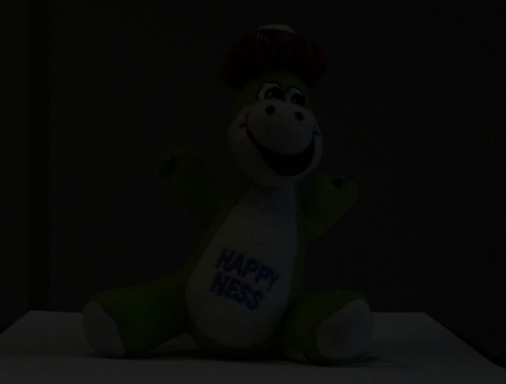
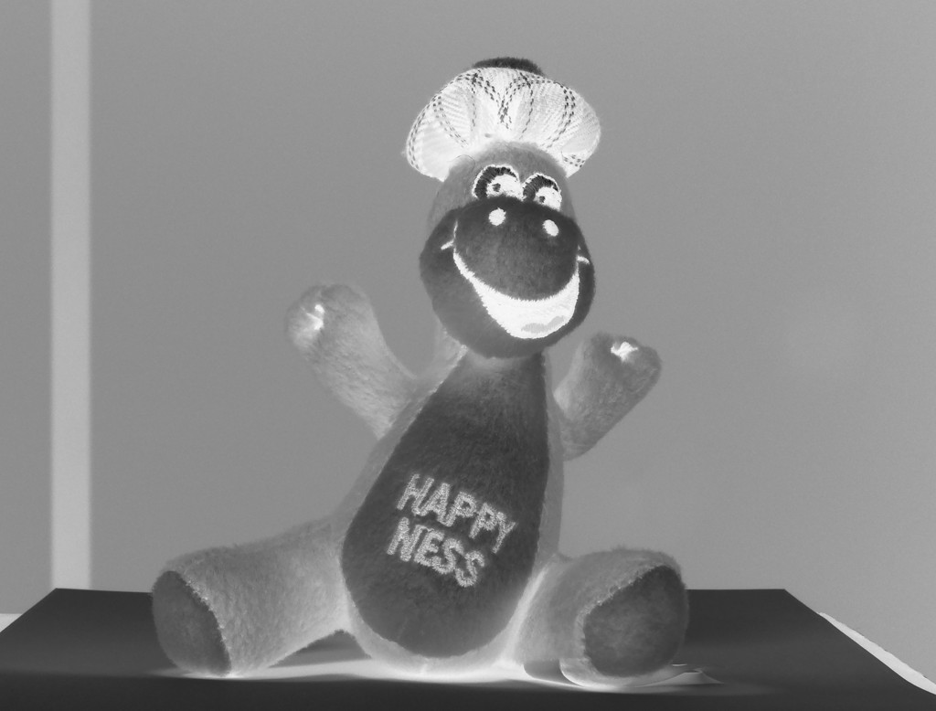
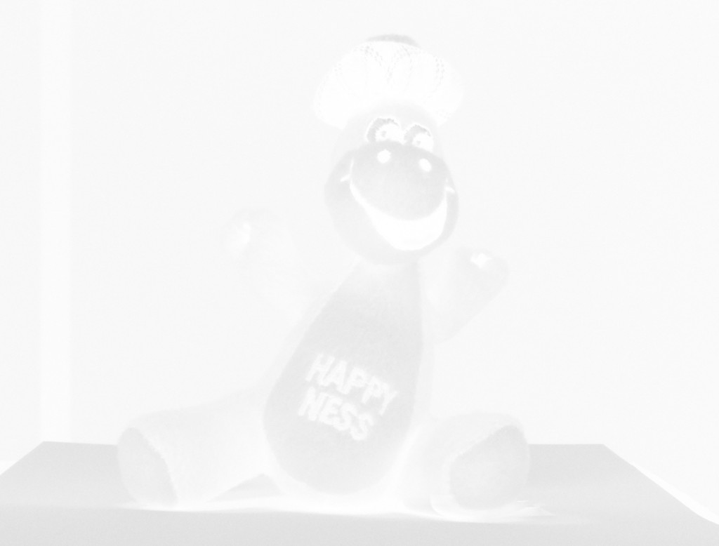
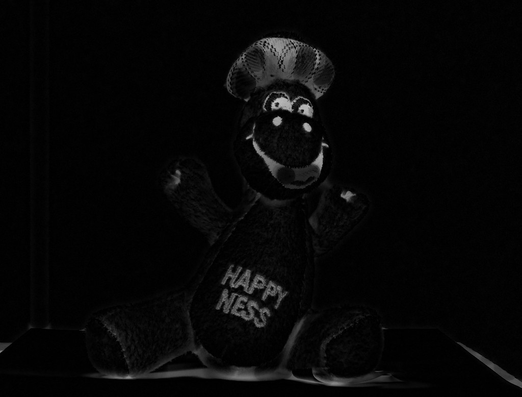
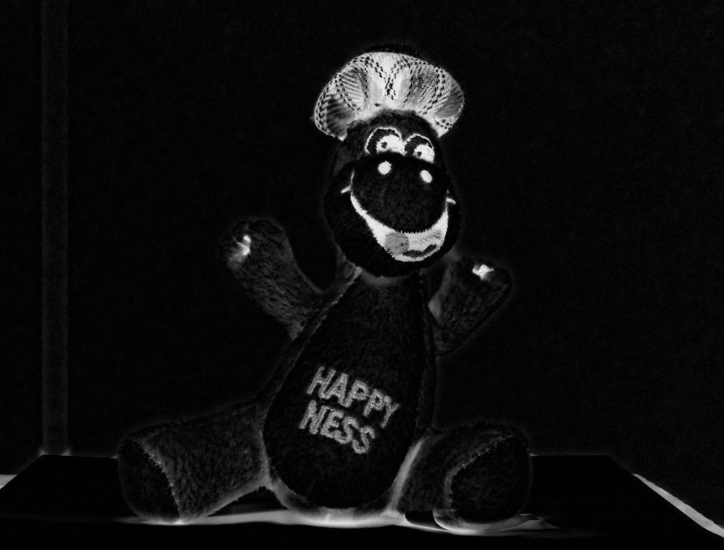
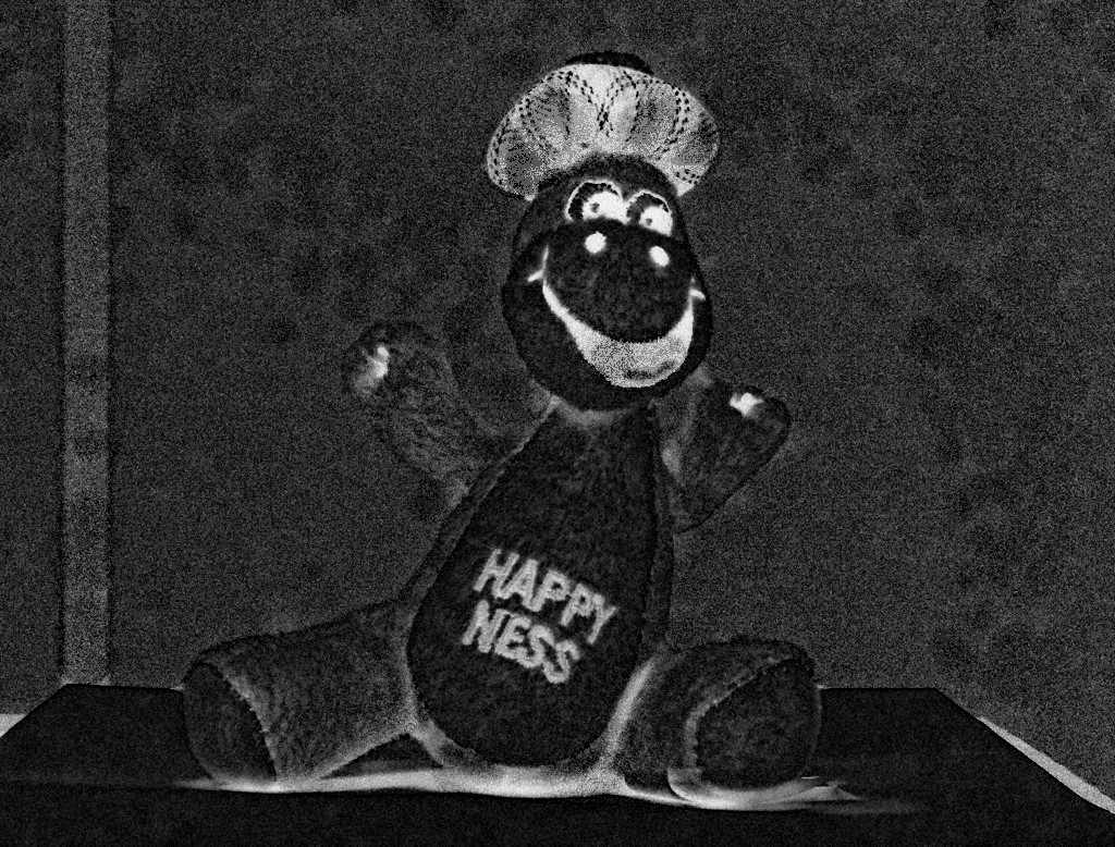
Let us focus on the extensions of top-hat operators and defined in section 5.4. Only the extended LIP-top-hat operator is insensitive to the LIP-addition of any constant lying in the interval . As the LIP-addition of a constant models a change of the camera exposure-time or of the source intensity, the logarithmic operator is expected to have a low sensitivity to such changes. In order to verify this assumption, an experiment has been conducted. An image of the same scene is acquired with two significantly different exposure-times. The scene is composed of a soft toy monster named “Nessie”, which is put down on a white support. (Figure 9). The first colour image (Figure 9a) is captured with a sufficient exposure-time of . It is therefore bright and highly-contrasted. Its luminance is denoted by and it is represented in the LIP-scale: i.e., the inverted greyscale (Figure 9c). The second colour image (Figure 9b) is captured with a too small exposure-time of , which makes it dark and lowly-contrasted. Its luminance is denoted by (Figure 9d). The extended top-hat operator is computed on both luminance images and . The resulting images are denoted by (Figure 9e) and (Figure 9f). It can be noticed that the extended top-hat in the dark image is much less contrasted than in the bright image . The extended top-hat operator is therefore sensitive to lighting changes caused by a variation of the camera exposure-time.
The other operator, the extended LIP-top-hat is then computed on both luminance images and . The resulting images are denoted by (Figure 9g) and (Figure 9h). It can be noticed that both results, and , are similar for the most-contrasted part of the scene (i.e, the foreground): the hat, the mouth of “Nessie”, the letters on its body, the bottom of its body and the contour of the white support. For the background (i.e. the very low-contrasted parts of the scene), there exist differences between the results in the bright image and in the dark image . They are due to the noise caused by the acquisition in the lowly-contrasted image (Figure 9b). However, such a noise also exists in the background of the extended top-hat of the dark image (Figure 9f), although it is hidden by some important amplitudes in . Indeed, when zooming in the background part of (Figure 9f) and rescaling its amplitude, the noise can be observed (Figure 9j). It is similar to the one observed in the extended LIP-top-hat of the dark image (Figure 9h).
In very low-contrasted parts of a dark image, the extended LIP-top-hat operator enhances the noise caused by the acquisition; i.e., when very few photons are captured by the camera sensor. However, in the most contrasted parts, this extended LIP-top-hat operator has the same amplitude in the bright image (Figure 9g) as in the dark image (Figure 9h). As a consequence, the extended LIP-top-hat operator is much more robust than the extended top-hat operator , to strong lighting variations caused by changes of camera exposure-time.
6.1.2 Map of Asplund distances with a tolerance to extrema
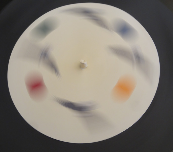
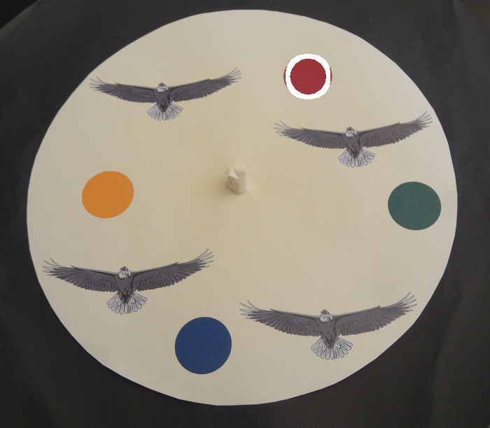
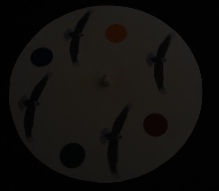
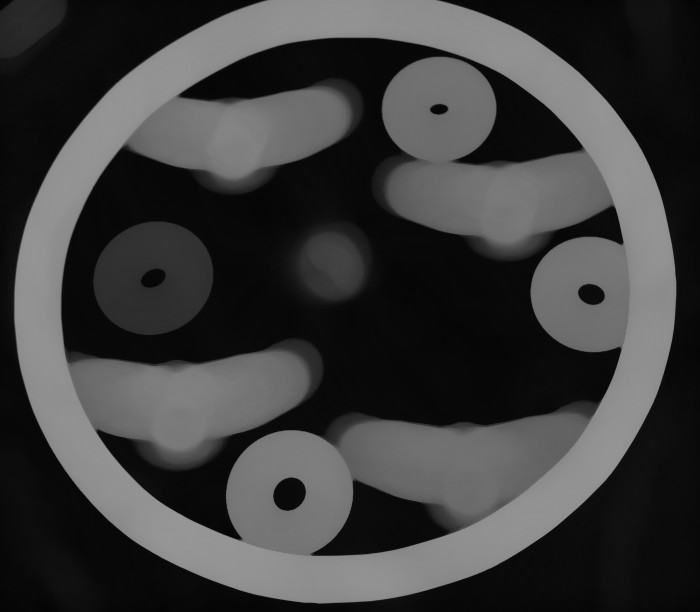
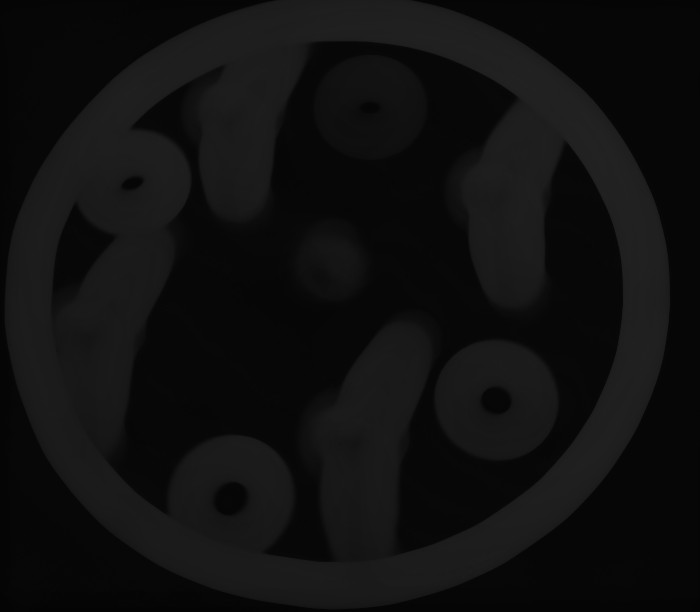
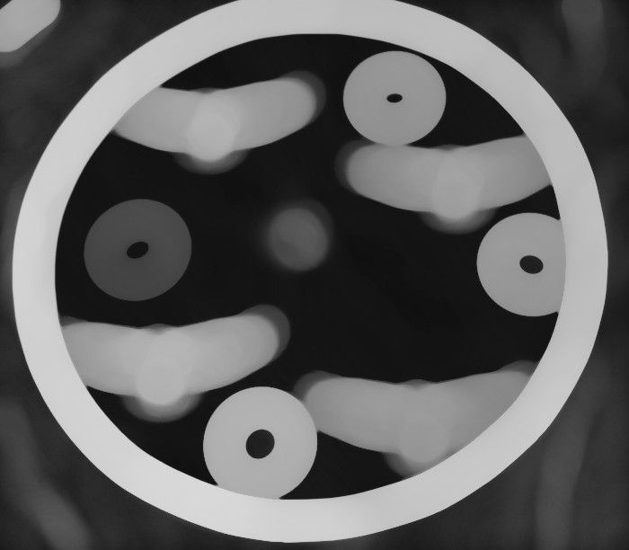
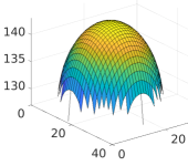
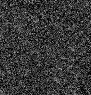
The map of LIP-additive Asplund distances with a tolerance to extrema, , defined in (326), is expected to be robust to strong lighting variations caused by different camera exposure-times. In order to verify this assumption, an experiment is performed with images of a moving object. In those images, the blur effect caused by the movement can be avoided by decreasing the camera exposure-time. However, this is done a the detriment of the image contrast. In Figure 10, a white disk with patterns is mounted on a turn table of a record player. The patterns include four small coloured disks and confounding shapes (i.e., the eagles). Firstly, in Figure 10a, an image of the static white disk is captured with an appropriate camera exposure-time of . This makes the image it well-contrasted. Then, the record player is started up at a speed of . With the same camera exposure-time as the one of , a first image is captured (Figure 10b). It is correctly contrasted but blurred which makes it useless to detect the coloured disks. In order to suppress the blur effect, the camera exposure-time is decreased to and a second image is captured (Figure 10c). This second image is not blurred but is darker than the image of the static disk (Figure 10b). In the luminance images, and , of those two differently contrasted images (Figure 10b) and (Figure 10c), the map of LIP-additive Asplund distances with a tolerance to extrema is compared to its equivalent in classical functional MM, , defined as follows:
| (554) |
The parameters and are defined as in proposition 5. In classical MM, the map of the static disk image (Figure 10d) is brighter than the map of the moving disk image (Figure 10e). However, in LMM, the maps of LIP-additive Asplund distances, with a tolerance, and which are applied to the static disk image (Figure 10f) and to the moving disk image (Figure 10g) are similarly contrasted. Contrary to the maps in classical MM, the LMM maps are therefore robust to strong lighting variations caused by different camera exposure-times.
6.2 Robustness to non-uniform lighting variations in images
In order to test the robustness to non-uniform lighting variations of a segmentation task, a LMM approach [49] is compared to other state-of-the-art methods [50, 51, 52]. The segmentation task consists of extracting vessels in eye fundus images coming from the test set of the DRIVE dataset [53]. However, the testing set is composed of olour eye fundus images which are well contrasted and do not present any significant non-uniform lighting variations. As a consequence, such variations were previously added to those images.
6.2.1 Adding lighting variations to the images
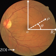
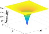
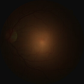
In a colour image , where , the non-uniform lighting variations are generated by LIP-adding a same darkening function to each of the three image components: , and . The darkening function is a 2D increasing function whose origin is located at the centre of the Zone of Interest (ZOI). The ZOI is assimilated to a circle of radius and centre , where (Figure 11a). Let and be the polar coordinates of the pixels from the circle centre . The darkening function is defined by (Figure 11b):
The intensity value s chosen so that the image is strongly darkened in its external part. The darkened image is then defined for each of its components as follows:
where is the floor function of the value . The floor function allows to save the darkened images in png or tif format in order to use them with different segmentation methods. Those darken images have a brighter area in their centre than elsewhere (Figure 11c).
6.2.2 Vessel segmentation method based on LMM
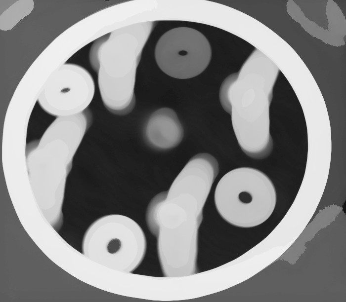
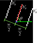
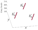
In [49, 19], a method based on Logarithmic Mathematical Morphology was introduced to segment vessels in eye fundus images. The colour images are converted to greyscale images in the LIP-scale thanks to the equation . In this inverted greyscale, the vessels appear as brighter than their surroundings. As in section 5.2, a bump detector is defined. It is based on a 2D probe composed of 3 parallel segments in the orientation and with the same length (Figure 12a). The probe origin is chosen as one of the extremities of the central segment . Its intensity is greater than the one of the left and right segments and (Figure 12b). These two segments are equidistant of the central one and the width of the probe is .
The left and right detectors and of (385) and (418) are now defined with the minimum , for any , as follows:
| (595) | |||||
| (628) | |||||
The map is defined as the pointwise infimum of the maps , and for each segment , and of the probe :
As the central segment must fully enter into the vessel relief, the infimum must be extracted and therefore in the previous equation, the map is used (see (192) and (259)). However, in order to reduce the effects of noise for the left and right segments, and , the maps with the minimum, and , are used (see (352)). As in (419), the bump detector map in orientation , , is defined by:
| (653) |
The bump detector map is expressed as the point-wise infimum of the maps in all the orientations :
| (654) |
As the vessel detection is a multi-scale problem, different probes, , of width and length will be used. The bump detector maps for the probes are then combined by point-wise infimum:
| (655) |
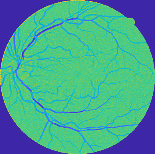
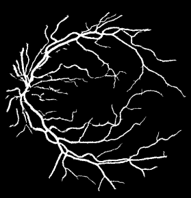
In the map of vesselness (Figure 13a), the vessels appear as valleys. They are extracted by a threshold such that of the ZOI area are considered as vessels (Figure 13b). probes with rientations between and are chosen. The width of the probe was chosen in order to be slightly greater than the largest vessel diameter. All the parameters and the experiments used to estimate them are given in [49].
Similarly to property 2, the following property holds777The proof of property 5 is in Supplementary Material.
Property 5.
The map of vesselness is therefore robust to uniform variations of light intensity or of camera exposure-time in an image . Indeed, such variations are modelled by the LIP-addition (or the LIP-subtraction) of a constant . The vessel segmentation by this LMM approach is therefore robust to such uniform lighting variations.
6.2.3 Comparison of the LMM approach with other methods
| Method | Images | AUC | Acc | Se | Sp | R. Diff. |
|---|---|---|---|---|---|---|
| LMM | initial | |||||
| dark | ||||||
| FR-UNet | initial | |||||
| dark | ||||||
| SGL | initial | |||||
| dark | ||||||
| RV-GAN | initial | |||||
| dark |
The robustness to non-uniform lighting variations will be tested for the previous approach and state-of-the-art approaches. As explained in section 6.2.1, a non-uniform lighting variation was generated by LIP-adding to the images a function which varies across the domain , in place of a constant . The 20 test images of the dataset were darkened.
For comparison purposes, the three best methods of vessel segmentation were selected in the DRIVE dataset using the ranking given in [54]. They are named FR-UNet [50], RV-GAN [51] and SGL (Study Group Learning) [52] and are based on Deep Learning architectures. FR-UNET is based on a multi-resolution U-Net architecture [55]. RV-GAN is composed of a multi-scale Generative Adversarial Network [56]. SGL is based on a U-Net consisting of an image enhancement module and a segmentation module. Those three methods have been tested on the test set using the pre-trained weights given by their authors. In table I, the performance of each method was evaluated by several indicators for the initial and the darkened images of the test set. The indicators are the mean values over the test set of the Area Under ROC Curve (AUC), Accuracy (Acc), Sensitivity (Se) and Specificity (Sp). Each indicator was computed for each image and the mean value was taken over the test set. The same groundtruth coming from the DRIVE dataset was used. The same program in MATLAB® language was used to estimate those indicators.
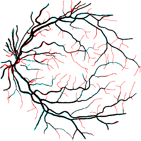
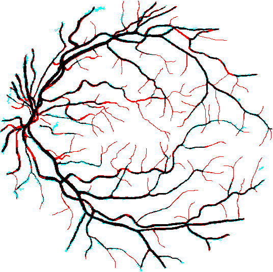
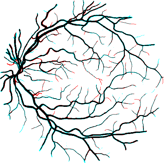


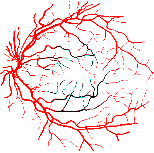
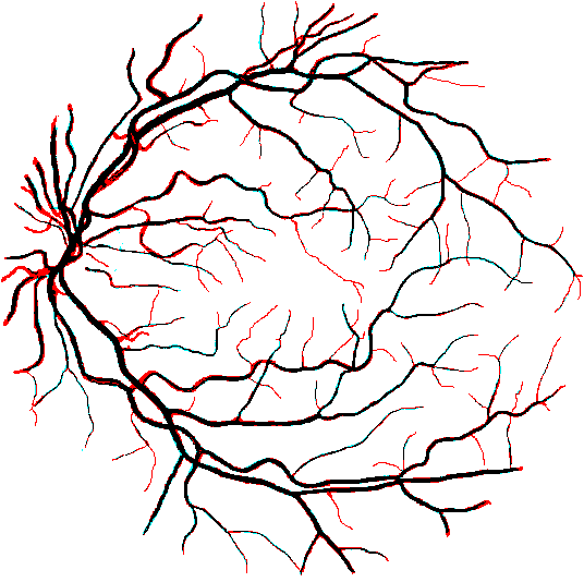
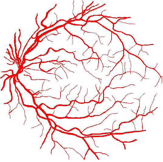
The relative difference between the AUC for the initial images and the darkened ones has been computed. The LMM approach obtains the smallest relative difference between AUC with . This is better than the other methods: FR-UNet (), SGL () and RV-GAN (). In Figure 14, one can notice that the LMM segmentations are much more similar between the initial test image (Figure 14a) and its darkened version (Figure 14b) than the segmentations with the other approaches. Indeed, in the initial images, the FR-UNet (Figure 14c), the SGL (Figure 14e) and the RV-GAN (Figure 14g) methods obtains good segmentation results. However, in the darken image, the FR-UNet (Figure 14d) and the SGL (Figure 14f) methods only segment the vessels in the brightest part located in the image centre. The RV-GAN approach does not segment the vessels (Figure 14h).
7 Conclusion
A new framework named Logarithmic Mathematical Morphology (LMM) has been presented. It allows to define Mathematical Morphology operations for images and functions with a upper bound value by using the Logarithmic Image Processing (LIP) vector space and its additive law . The sum between two functions and with an upper bound value is smaller than this upper bound value. The amplitude of the second function, namely the structuring function, varies according to the intensity of the function and in a way which is physically justified. Such a physical property comes from the LIP model which is defined thanks to the transmittance law and which is coherent with the human vision. The new framework, namely the LMM, allows the definition of morphological operators which are robust to lighting variations modelled by the LIP-additive law . Those variations correspond to a change of light intensity or of camera exposure-time. Experiments have shown that those operators are robust to such uniform lighting variations and perform better than usual morphological operations defined with the usual additive law . With non-uniform lighting variations, a LMM approach for vessel segmentation in eye-fundus images is more robust than three state-of-the-art methods based on deep-learning, namely FR-UNet, SGL and RVGAN. LMM framework paves the way for the definition of morphological operators and neural nets [20] allowing a robust analysis of images acquired in uncontrolled lighting variations. Such variations occur in numerous practical applications (outdoor scenes, industry, medicine, remote-sensing, etc.)
Acknowledgments
The author would like to thank Prof. Michel Jourlin for his careful re-reading of the manuscript.
References
- [1] G. Matheron, Random sets and integral geometry, ser. Wiley ser. in probability and math. statis. New York, NY, USA: Wiley, 1975.
- [2] J. Serra and N. Cressie, Image Analysis and Mathematical Morphology. Orlando, FL, USA: Academic, 1982, vol. 1.
- [3] S. R. Sternberg, “Parallel architectures for image processing,” in COMPSAC 79. Proc. Comput. Softw. and The IEEE Comput. Soc.’s Third Int. Appl. Conf., Nov. 1979, pp. 712–717.
- [4] S. R. Sternberg, “Grayscale morphology,” Computer Vision, Graphics, and Image Processing, vol. 35, no. 3, pp. 333 – 355, 1986.
- [5] P. Maragos, “A representation theory for morphological image and signal processing,” IEEE Trans. Pattern Anal. Mach. Intell., vol. 11, no. 6, pp. 586–599, Jun. 1989.
- [6] H. J. A. M. Heijmans, “Theoretical aspects of gray-level morphology,” IEEE Trans. Pattern Anal. Mach. Intell., vol. 13, no. 6, pp. 568–582, Jun. 1991.
- [7] H. Heijmans and C. Ronse, “The algebraic basis of mathematical morphology I. Dilations and erosions,” Comput. Vision Graphics and Image Process., vol. 50, no. 3, pp. 245 – 295, Jun. 1990.
- [8] H. Heijmans, Morphological image operators, ser. Adv. Imag. Electron Phys.: Suppl. San Diego, CA, USA: Academic, 1994, no. vol. 25.
- [9] M. Jourlin and J. Pinoli, “A model for logarithmic image-processing,” J. Microsc., vol. 149, no. 1, pp. 21–35, Jan. 1988.
- [10] J. Brailean, B. Sullivan, C. Chen, and M. Giger, “Evaluating the EM algorithm for image processing using a human visual fidelity criterion,” in IEEE Int. Conf. Acoustics, Speech, Signal Process., Apr. 1991, pp. 2957–2960 vol.4.
- [11] J. Z. Sun, G. I. Wang, V. K. Goyal, and L. R. Varshney, “A framework for bayesian optimality of psychophysical laws,” Journal Math Psychology, vol. 56, no. 6, pp. 495 – 501, 2012.
- [12] L. R. Varshney and J. Z. Sun, “Why do we perceive logarithmically?” Significance, vol. 10, no. 1, pp. 28–31, 2013.
- [13] M. Jourlin, “Chapter One - Gray-Level LIP Model. Notations, Recalls, and First Applications,” in Logarithmic Image Processing: Theory and Applications, ser. Adv. Imag. Electron Phys., M. Jourlin, Ed. Elsevier, 2016, vol. 195, pp. 1 – 26.
- [14] E. H. Land, “The retinex theory of color vision,” Sci. Am., vol. 237, no. 6, pp. 108–129, 1977. [Online]. Available: www.jstor.org/stable/24953876
- [15] R. Kimmel, M. Elad, D. Shaked, R. Keshet, and I. Sobel, “A Variational Framework for Retinex,” Int. J. Comput. Vision, vol. 52, no. 1, pp. 7–23, Apr. 2003.
- [16] M. Jourlin and J. Pinoli, “Logarithmic image processing: The mathematical and physical framework for the representation and processing of transmitted images,” ser. Adv. Imag. Electron Phys. Elsevier, 2001, vol. 115, pp. 129 – 196.
- [17] M. Jourlin, Logarithmic Image Processing: Theory and Applications, ser. Adv. Imag. Electron Phys. Elsevier, 2016, vol. 195.
- [18] G. Noyel, “Logarithmic mathematical morphology: A new framework adaptive to illumination changes,” ser. Lect. Notes Comput. Sci., vol. 11401. Springer, 2019, pp. 453–461.
- [19] ——, “Morphological and logarithmic analysis of large image databases,” Dissertation of Accreditation to supervise Research, Université de Reims Champagne-Ardenne, France, Jun. 2021. [Online]. Available: https://tel.archives-ouvertes.fr/tel-03343079
- [20] G. Noyel, E. Barbier-Renard, M. Jourlin, and T. Fournel, “Logarithmic morphological neural nets robust to lighting variations,” ser. Lect. Notes Comput. Sci. Springer, 2022, pp. 462–474.
- [21] F. Meyer, “Iterative image transformations for an automatic screening of cervical smears.” J. Histochemistry & Cytochemistry, vol. 27, no. 1, pp. 128–135, 1979.
- [22] M. Jourlin and N. Montard, “A logarithmic version of the top-hat transform in connection with the Asplund distance,” Acta Stereologica, vol. 16, pp. 201 – 208, 1997.
- [23] E. Zaharescu, “Morphological enhancement of medical images in a logarithmic image environment,” in 2007 15th Int. Conf. Digit. Signal Process., Jul. 2007, pp. 171–174.
- [24] S. Beucher and F. Meyer, “The morphological approach to segmentation: The watershed transformation,” in Math. Morphology in Image Process. New York, NY, USA: Marcel Dekker, 1993, pp. 433–481.
- [25] S. Beucher, “Image segmentation and mathematical morphology,” Thèse, Ecole Nat. Supérieure Mines Paris, Fr., Jun. 1990. [Online]. Available: https://pastel.archives-ouvertes.fr/tel-00108290
- [26] D. G. Lowe, “Distinctive image features from scale-invariant keypoints,” Int. J. Comput. Vision, vol. 60, no. 2, pp. 91–110, Nov. 2004.
- [27] P. Salembier, A. Oliveras, and L. Garrido, “Antiextensive connected operators for image and sequence processing,” IEEE Trans. Image Process., vol. 7, no. 4, pp. 555–570, Apr. 1998.
- [28] P. Monasse and F. Guichard, “Fast computation of a contrast-invariant image representation,” IEEE Trans. Image Process., vol. 9, no. 5, pp. 860–872, May 2000.
- [29] N. Passat, B. Naegel, F. Rousseau, M. Koob, and J.-L. Dietemann, “Interactive segmentation based on component-trees,” Pattern Recogn, vol. 44, no. 10, pp. 2539 – 2554, 2011.
- [30] Y. Xu, T. Géraud, and L. Najman, “Connected filtering on tree-based shape-spaces,” IEEE Trans. Pattern Anal. Mach. Intell., vol. 38, no. 6, pp. 1126–1140, Jun. 2016.
- [31] G. Noyel and M. Jourlin, “Region homogeneity in the logarithmic image processing framework: Application to region growing algorithms,” Image Anal. & Stereology, vol. 38, no. 1, pp. 43–52, 2019.
- [32] G. Birkhoff, Lattice Theory, 3rd ed., ser. Amer. Math. Soc. Colloq. Publications. Providence, RI: AMS, 1967, vol. 25.
- [33] G. J. F. Banon and J. Barrera, “Decomposition of mappings between complete lattices by mathematical morphology, part I: General lattices,” Signal Process., vol. 30, no. 3, pp. 299 – 327, Feb. 1993.
- [34] J. Serra, Image analysis and mathematical morphology: Theoretical advances. San Diego, CA, USA: Academic, 1988, vol. 2.
- [35] C. Ronse and H. Heijmans, “The algebraic basis of mathematical morphology: II. Openings and closings,” CVGIP: Image Understanding, vol. 54, no. 1, pp. 74 – 97, 1991.
- [36] P. Soille, Morphological Image Analysis: Principles and Applications, 2nd ed. New York: Springer-Verlag, 2003.
- [37] L. Najman and H. Talbot, Mathematical Morphology: From Theory to Applications, 1st ed. Hoboken, NJ, USA: Wiley, 2013.
- [38] F. Meyer, Topographical Tools for Filtering and Segmentation 1: Watersheds on Node- or Edge-weighted Graphs. USA: Wiley, 2019.
- [39] ——, Topographical Tools for Filtering and Segmentation 2: Flooding and Marker-based Segmentation on Node- or Edge-weighted Graphs. Hoboken, NJ, USA: Wiley, 2019.
- [40] N. Bouaynaya and D. Schonfeld, “Theoretical foundations of spatially-variant mathematical morphology part II: Gray-level images,” IEEE Trans. Pattern Anal. Mach. Intell., vol. 30, no. 5, pp. 837–850, May 2008.
- [41] R. Verdú-Monedero, J. Angulo, and J. Serra, “Anisotropic morphological filters with spatially-variant structuring elements based on image-dependent gradient fields,” IEEE Trans. Image Process., vol. 20, no. 1, pp. 200–212, Jan. 2011.
- [42] J. J. van de Gronde and J. B. T. M. Roerdink, “Group-invariant colour morphology based on frames,” IEEE Trans. Image Process., vol. 23, no. 3, pp. 1276–1288, Mar. 2014.
- [43] O. Merveille, H. Talbot, L. Najman, and N. Passat, “Curvilinear structure analysis by ranking the orientation responses of path operators,” IEEE Trans. Pattern Anal. Mach. Intell., vol. 40, no. 2, pp. 304–317, Feb 2018.
- [44] M. Jourlin and J.-C. Pinoli, “Image dynamic range enhancement and stabilization in the context of the logarithmic image processing model,” Signal Process., vol. 41, no. 2, pp. 225 – 237, Jan. 1995.
- [45] P. Maragos and R. Schafer, “Morphological filters–part II: Their relations to median, order-statistic, and stack filters,” IEEE Trans. Acoust., Speech, Signal Process., vol. 35, no. 8, pp. 1170–1184, Aug. 1987.
- [46] G. Noyel and M. Jourlin, “Double-sided probing by map of Asplund’s distances using logarithmic image processing in the framework of mathematical morphology,” ser. Lect. Notes Comput. Sci., vol. 10225. Springer, 2017, pp. 408–420.
- [47] ——, “Functional asplund metrics for pattern matching, robust to variable lighting conditions,” Image Analysis & Stereology, vol. 39, no. 2, pp. 53–71, 2020.
- [48] G. Noyel, “A link between the multiplicative and additive functional asplund’s metrics,” ser. Lect. Notes Comput. Sci., vol. 11564. Springer, 2019, pp. 41–53.
- [49] G. Noyel, C. Vartin, P. Boyle, and L. Kodjikian, “Retinal vessel segmentation by probing adaptive to lighting variations,” in IEEE 17th Int. Sympo. Biomed. Imag. (ISBI), 2020, pp. 1246–1249.
- [50] W. Liu, H. Yang, T. Tian, Z. Cao, X. Pan, W. Xu, Y. Jin, and F. Gao, “Full-resolution network and dual-threshold iteration for retinal vessel and coronary angiograph segmentation,” IEEE J. Biomed. Health Inform., vol. 26, no. 9, pp. 4623–4634, 2022.
- [51] S. A. Kamran, K. F. Hossain, A. Tavakkoli, S. L. Zuckerbrod, K. M. Sanders, and S. A. Baker, “RV-GAN: Segmenting retinal vascular structure in fundus photographs using a novel multi-scale generative adversarial network,” ser. Lect. Notes Comput. Sci., vol. 12908. Springer, 2021, pp. 34–44.
- [52] Y. Zhou, H. Yu, and H. Shi, “Study group learning: Improving retinal vessel segmentation trained with noisy labels,” ser. Lect. Notes Comput. Sci., vol. 12901. Springer, 2021, pp. 57–67.
- [53] J. Staal, M. D. Abramoff, M. Niemeijer, M. A. Viergever, and B. van Ginneken, “Ridge-based vessel segmentation in color images of the retina,” IEEE Trans. Med. Imag., vol. 23, no. 4, pp. 501–509, Apr. 2004.
- [54] (2023) Retinal vessel segmentation on DRIVE. [Online]. Available: https://paperswithcode.com/sota/retinal-vessel-segmentation-on-drive
- [55] O. Ronneberger, P. Fischer, and T. Brox, “U-net: Convolutional networks for biomedical image segmentation,” ser. Lect. Notes Comput. Sci., vol. 9351. Springer, 2015, pp. 234–241.
- [56] I. J. Goodfellow, J. Pouget-Abadie, M. Mirza, B. Xu, D. Warde-Farley, S. Ozair, A. Courville, and Y. Bengio, “Generative adversarial nets,” in NIPS’14, 2014, p. 2672–2680.