Dark Matter Velocity Distributions: Comparing Numerical Simulations to Analytic Results

Abstract

We test the consistency of dark matter velocity distributions obtained from dark matter-only numerical simulations with analytic predictions, using the publicly available Via Lactea 2 dataset as an example. We find that, well inside the scale radius, the velocity distribution obtained from numerical simulation is consistent with a function of a single integral of motion – the energy – and moreover is consistent with the result obtained from Eddington inversion. This indicates that the assumptions underlying the analytic result, namely, spherical symmetry, isotropy, and a static potential, are sufficiently accurate to govern the coarse properties of the velocity distribution in the inner regions of the halo. We discuss implications for the behavior of the high-velocity tail of the distribution, which can dominate dark matter annihilation from a $p$- or $d$-wave state.

I Introduction

The velocity distribution of particle dark matter (DM) in (sub)halos is an important input to dark matter direct and indirect detection searches. There are two main strategies for studying this distribution: large $N$ numerical simulations [1, 2, 3, 4], and analytic analyses of the phase space distribution [5, 6]. The advantage of simulations is that they do not require the use of approximations, such as spherical symmetry or isotropy, and incorporate the details of the merger history. The advantage of analytic analyses, apart from computational simplicity, is that they allow one to learn broad lessons which apply beyond the details of an individual simulation. Our goal in this work is to investigate the extent to which the results of numerical simulations of the dark matter velocity distribution match the general predictions of analytic analyses.

The answer to this question has significant implications for dark matter detection strategies. The connection between the dark matter velocity distribution and direct detection has been well studied [7]. For many dark matter candidates, it is only the high speed tail of the DM distribution which can deposit enough energy in the detector to produce a recoil above threshold. Moreover, the velocity distribution affects the annual modulation of a direct detection signal [8]. The connection between the DM velocity distribution and indirect detection has been less well studied because, if the DM annihilation cross section is velocity-independent (the most commonly studied scenario), then the annihilation rate will depend only on the density distribution, not the velocity distribution. But there are a variety of particle physics models in which the annihilation cross section is velocity-dependent, and in these cases, the astrophysical $J$-factor which controls the annihilation rate in any particular astrophysical target will depend in detail on the velocity distribution [9, 10, 11, 12].

For example, for models of $p$- or $d$-wave dark matter annihilation, the dark matter indirect detection signal receives an enhanced contribution from the annihilation of particles in the high-speed tail of the velocity distribution. In numerical simulations, one finds that in any radial shell, the velocity distribution is well fit by a Maxwell-Boltzmann distribution with an exponential tail (see, for example, [13, 14]). On the other hand, analytic analyses suggest that, under certain assumptions, the high-speed tail falls off only as a power law near the center of the halo (see, for example, [15, 16]). Although the broad features of these distributions are similar, the differences are significant. If the velocity distribution only falls off as a power-law, then the power-law enhancement of the cross section in the case of $p$-/$d$-wave annihilation can compensate, causing the indirect detection signal to be dominated by the small fraction of particles in the high-speed tail. This tail is much less significant if the velocity-distribution exhibits an exponential falloff at high speed. It is thus important to know if the results of numerical simulations, though well fit by a Maxwell-Boltzmann distribution, are generally consistent with the predictions of analytic analyses. Particularly since the high-speed tail is necessarily relatively poorly sampled in numerical simulations, it is helpful to know if analytic results for the asymptotic behavior of the tail can be trusted. More generally, if the results of numerical simulations are consistent with those of analytic analyses, then credence is lent to the idea that the approximations which underlie the analytic analyses are sufficiently good.

In this work, we consider the publicly available results of the Via Lactea 2 (VL-2) DM-only numerical simulation [3], consisting of $10^{5}$ particles randomly drawn from the $10^{9}$ particles in their sample. We find that, for radial distances less than half the scale radius, the velocity-distribution inferred from these particles is broadly consistent with being a function of a single integral of motion – the energy. This is the result predicted from analytic analyses, under the assumptions of spherical symmetry, isotropy, and time-invariance. Although these assumptions are not exact, deviations from these assumptions are apparently small enough that they do not have a large effect on coarse features of the velocity distribution in the inner regions of the halo. More specifically, we find that the velocity distribution obtained from VL-2 is consistent with the result obtained from Eddington inversion.

The plan of this paper is as follows. In Section II, we will review results from an analytic analysis of the phase distribution. We compare these to publicly-available results obtained from the VL-2 numerical simulation in Section III. We conclude in Section IV.

II Analytic Analysis of the Phase Space Distribution

In general, the velocity distribution $f(\vec{r},\vec{v},t)$ is a function of seven variables. We begin with four initial assumptions:

1. the DM velocity distribution (as well as the distribution of any baryonic matter) is spherically symmetric,

2. the DM velocity distribution (as well as the distribution of any baryonic matter) is independent of time,

3. each DM particle is subject only to central forces which depend only on its radial position,

4. and the DM velocity distribution is isotropic (optional).

If the only relevant forces are gravitational, then assumptions (i) and (ii) together imply assumption (iii). Although this is the standard scenario, in the interests of generality, we will retain (iii) as an independent assumption. Of course, none of these assumptions will be exactly true. Our goal will be to examine the consequences of these assumptions, and compare the resulting predictions to results from numerical simulations, in which none of these assumptions are made.

Assumptions (i)-(iii) imply that the velocity-distribution is only a function of three variables: $r$, $v_{r}$ and $v_{\perp}$, where $r=|\vec{r}|$, $v_{r}=\vec{v}\cdot\hat{r}$, and $v_{\perp}=\sqrt{\vec{v}^{2}-v_{r}^{2}}$. Moreover, these three assumptions imply that each dark matter particle may be thought of as moving under the influence of a single time-invariant central potential. $\vec{r}$ and $\vec{v}$ are thus functions of time and six integrals of motion.

Two integrals of motion determine the plane of motion, and another determines the orientation of the orbit in the plane. The remaining three are the energy, the magnitude of the angular momentum, and a constant $t_{0}$ which identifies the time zero-point. Spherical symmetry implies that $f$ is independent of the first three integrals of motion, and thus is a function of only three variables, as expected. Liouville’s theorem further implies that the phase space density is invariant under time-translation, so $f$ is also independent of $t_{0}$. Thus, assumptions (i)-(iii) imply that $f$ is a function only of the energy and the magnitude of the angular momentum. If assumption (iv) also holds, than $f$ depends only on $r$ and $v=|\vec{v}|$, or equivalently, that $f$ is a function of energy alone.

Given assumptions (i)-(iii), the density distribution is a function only of $r$, given by

$$\rho(r) = \int_{0}^{v_{esc}(r)}d^{2}v_{\perp}dv_{r}~{}f(r,v_{r},v_{\perp}),$$ (1)

$$= 2\sqrt{2}\pi\int_{0}^{\sqrt{2}r\sqrt{\Phi(\infty)-\Phi(r)}}dL~{}\int_{L^{2}/2r^{2}+\Phi(r)}^{\Phi(\infty)}dE~{}\frac{L}{r^{2}}\frac{1}{\sqrt{E-\frac{L^{2}}{2r^{2}}-\Phi(r)}}f(E,L),$$

where $E$ and $L$ are the energy and angular momentum per unit mass, respectively. $\Phi$ is the gravitational potential, and

$$E = \frac{1}{2}\left(v_{r}^{2}+v_{\perp}^{2}\right)+\Phi(r),$$

$$L = rv_{\perp},$$

$$v_{esc}(r) = \sqrt{2\left(\Phi(\infty)-\Phi(r)\right)}.$$ (2)

If $f$ is independent of $L$, then one may perform the integral over $L$, yielding

$$\rho(r) = 4\sqrt{2}\pi\int_{\Phi(r)}^{\Phi(\infty)}dE~{}\sqrt{E-\Phi(r)}~{}f(E).$$ (3)

We can use these formulae to test if the velocity distribution is determined by these two integrals of motion. If assumptions (i)-(iv) hold, and $f$ depends only on $E$, then in any thin radial shell of volume $dV$, the number of particles within the energy range $[E,E+dE]$ is given by

$$N(E,r) = \left[4\sqrt{2}\pi\sqrt{E-\Phi(r)}~{}dE~{}dV\right]f(E).$$ (4)

Scaling out the factor in brackets, one can use the particle count per energy bin in a numerical simulation to determine $f(E)$ for each radial bin. If $f$ only depends on $E$, then these functions will be identical, differing only in the range of energies (from $\Phi(r)$ to $\Phi(\infty)$) which are sampled in each radial shell.

If only assumptions (i)-(iii) are good approximations, then $f$ will depend on $E$ and $L$. The integral over $L$ is then non-trivial, and the rescaling above would not remove all radial dependence. As a result, the functions $f(E)$ found in different radial bins would not agree. In that case, one would use the particle count in radial bins and in bins of $E$ and $L$ in order to determine $f(E,L)$, after rescaling by the appropriate function of $E$, $L$ and $\Phi(r)$ found in eq. 1. But if even assumptions (i)-(iii) are not good approximations, then $f$ would not be expected to depend only on $E$ and $L$. In this case, even the functions $f(E,L)$ obtained from the particles counts in different radial bins would not agree.

In particular, if we derive the velocity distribution from numerical simulation data in two non-overlapping radial bins, then these velocity distributions have support over disjoint regions of phase space which are not related by spherical symmetry, and are a priori independent. What relates them is the fact that, given our assumptions, the integrals of motion $E$ and $L$ remain constant as a particle moves from one region of phase space to another. This need not be true if assumptions (i)-(iii) do not hold, as energy or angular momentum could be transferred from one particle to another.

III Comparison to Numerical Simulation

We consider the Via Lactea 2 DM-only simulation [3], consisting of $10^{9}$ particles. If fit to a generalized Navarro-Frenk-White (gNFW) profile of the form $\rho(r)=\rho_{s}/[(r/r_{s})^{\gamma}(1+r/r_{s})^{3-\gamma}]$ [17], the best fit value for the inner slope of the halo is $\gamma=1.24$, with a scale radius of $r_{s}=28.1~{}{\rm kpc}$ and a scale density $\rho_{s}=0.0035M_{\odot}/{\rm pc}^{3}$. The radius of convergence is $0.38~{}{\rm kpc}$, and is not expected to affect our results. We use the $10^{5}$ randomly selected particles which have been made publicly available. Fitting the enclosed mass of this subset of particles as a function of radius to a gNFW profile with $\gamma=1.24$ yields $\chi^{2}/dof=0.56$ (using 9 radial bins extending between $0.05r_{s}$ and $0.5r_{s}$). This indicates that the publicly available points do indeed constitute a representative sample which may be used to study the velocity distribution of this halo.

For simplicity, we use the dimensionless variable $\tilde{r}\equiv r/r_{s}$. We focus on the region $\tilde{r}<0.5$, which lies well within the scale radius, and for which we expect deviations from spherical symmetry and isotropy to be relatively small [18]. Understanding this region should give us a good understanding of the dark matter velocity distribution in the region of phase space most relevant for indirect detection, as dark matter annihilation is concentrated in the innermost regions of the halo, especially if the inner slope is relatively steep.

We divide the range $\tilde{r}<0.5$ into 5 radial shells (A-E), and in each, we estimate deviations from spherical symmetry and isotropy. In particular, we expand the density distribution in spherical harmonics and compute the associated expansion coefficients $a_{\ell m}$ for $\ell\leq 1$. We also compute the anisotropy coefficient $\beta\equiv 1-[\langle v_{\perp}^{2}\rangle/2\langle v_{r}^{2}\rangle]$. We define the radial extent of each region, and present the $a_{\ell m}$ and $\beta$ (with uncertainty) in Table 1. In each region, the velocity distribution is consistent with isotropy, and the dipole terms in the density distribution are relatively small.

region	$a_{00}$	$a_{10}$	Re $a_{11}$	Im $a_{11}$	$\beta$
$0<\tilde{r}<0.1$ (A)	$0.28$	$0.0028$	$0.0095$	$0.0000198$	$0.04\pm 2$
$0.1<\tilde{r}<0.2$ (B)	$0.28$	$0.01$	$0.01$	$0.0024$	$0.025\pm 2$
$0.2<\tilde{r}<0.3$ (C)	$0.28$	$0.01$	$0.007$	$0.027$	$0.14\pm 1.5$
$0.3<\tilde{r}<0.4$ (D)	$0.28$	$-0.005$	$0.008$	$0.02$	$0.16\pm 1.4$
$0.4<\tilde{r}<0.5$ (E)	$0.28$	$0.001$	$-0.015$	$0.022$	$0.13\pm 1.4$

Table 1: The radial extent of each of the five regions considered, along with the $a_{\ell m}$ ($\ell\leq 1$) and $\beta$.

We now investigate the extent to which the velocity distribution in the range $\tilde{r}<0.5$ can be well-represented as a function of energy alone. We divide each region into two subregions (denoted “1” (inner) and “2” (outer)) at the radial midpoint. Within each region, we choose a common energy binning for both subregions. In each subregion, we then determine the velocity distribution $f_{i}$ in the $i$th energy bin using the relation $f_{i}=N_{i}/[4\sqrt{2}\pi\sqrt{E-\Phi(\tilde{r})}\Delta E\Delta V]$, where $N_{i}$ is the number of particles in that energy bin, $\Delta E$ is the width of the energy bin, and $\Delta V$ is the spatial volume of the subregion. Here, $E$ is evaluated at the midpoint of the energy bin, and $\Phi(\tilde{r})$ is taken to be the average value of the potential over all particles in the subregion, assuming that the density distribution follows a gNFW form with $\gamma=1.24$. Note, we ignore energy bins for which $E_{avg}-\Phi_{avg}(\tilde{r})<0$. More generally, because the scaling factor in eq. 4 is averaged over the energy and spatial bin, there will be associated binning error in the resulting velocity distribution.

We then compare the values of $f(E)$ in the two subregions, to see if they are statistically consistent. Our results for the 5 pairs of subregions are presented in Table 2. We generally find consistency, indicating that, to a good approximation, the dependence of the velocity distribution on $r$ and $v$ arises from the dependence of $E$ on both.

pair	# of energy bins	$\chi^{2}/dof$
A1,A2	$8$	$0.92$
B1,B2	$10$	$1.42$
C1,C2	$9$	$0.71$
D1,D2	$8$	$1.11$
E1,E2	$10$	$0.95$

Table 2: For each region A through E, the number of energy bins used, and the $\chi^{2}/dof$ between $f(E)$ of the two subregions.

Finally, we can compare the $f(E)$ found in these ten subregions to the analytic expression one would obtain from Eddington inversion assuming a gNFW profile with inner slope of $\gamma=1.24$. Essentially, Eddington inversion amounts to inverting eq. 3 with an inverse Abel integral transform, allowing one to numerically solve for $f(E)$, given an ansatz for $\rho(r)$. For simplicity, we define the constant $E_{0}=4\pi G_{N}\rho_{s}r_{s}^{2}$, and the dimensionless quantities $\tilde{E}=E/E_{0}$, $\tilde{f}=f/(\rho_{s}E_{0}^{-3/2})$. We plot $\tilde{f}(\tilde{E})$ in the ten subregions, along with the analytic result (obtained using Eddington inversion for the case of a gNFW profile with $\gamma=1.25$ [15]), in Figure 1. The velocity distribution obtained from VL-2 data is consistent with the result obtained from Eddington inversion. Given this consistency, there is little to be gained from attempting to determine the dependence of the velocity distribution on angular momentum, given this limited data set.

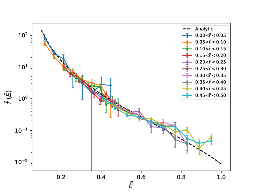
Figure 1: $\tilde{f}(\tilde{E})$ for ten radial bins from 0 to $0.5\tilde{r}_{s}$, with each bin of width $0.05\tilde{r}_{s}$, as labelled. Also plotted (dashed) is the analytic result obtained from Eddington inversion [15], assuming $\gamma=1.25$.

IV Conclusion

We have compared the dark matter halo velocity distribution found in DM-only numerical simulations to analytic predictions, using the publicly-available Via Lactea 2 dataset as an example. We have found them to be broadly consistent in the region lying well inside the scale radius. In particular, we have found that the velocity distribution found in numerical simulation is well described as a function of a single integral of motion – the energy. This is consistent with analytic predictions in the case in which the dark matter distribution is spherically symmetric, isotropic and time-invariant. More specifically, the velocity-distribution obtained from numerical simulation data is a good fit to the result obtained from Eddington inversion, well inside the scale radius.

Of course, there are certainly deviations from spherical symmetry, isotropy and time-invariance [19, 20], and the velocity distribution in a localized region will be significantly affected by the recent merger history [21, 22, 23], etc. Such deviations are especially important in the context of direct detection experiments, for which experimental sensitivity depends on the dark matter velocity-distribution at a particular location in the Milky Way halo. But our result implies that deviations from these approximations do not dramatically alter the broad features of the velocity distribution which one obtains from analytic methods, when averaged over sufficiently large scales. These features are more important in the context of indirect detection, where one is interested in dark matter annihilation within an entire halo or subhalo.

Deviations from spherical symmetry and time-invariance can certainly be important in the context of indirect detection as well, particularly in relation to the formation and disruption of substructure [24, 25, 26]. We have not attempted to consider this issue here, though it would be an interesting topic of future work. However, we have considered the application of our results to the case of dark matter annihilation from a $p$- or $d$-wave initial state, for which the form of the velocity distribution is important. In these scenarios, the effect of substructure is expected to be relatively mild [27].

Because the $p$-wave annihilation cross section scales as $(v/c)^{2}$, the contribution of the high-speed tail of the velocity distribution is enhanced, and it becomes important to know how strongly the velocity distribution is suppressed at high speed. Since the tail of the distribution will be least well-sampled in a numerical simulation, it is helpful to be able to gain intuition from analytic results. If the velocity-distribution is a function of energy alone, then within a power-law cusp, the velocity-distribution will generally fall off only as a power of velocity [15], not exponentially (as one would expect if the velocity-distribution were Maxwell-Boltzmann). Indeed, these results suggest that for a dark matter halo of gNFW form with $\gamma=1.24$ (as in the VL-2 halo), $d$-wave annihilation (which scales as $(v/c)^{4}$) even within the cusp is dominated by the most energetic particles, which explore the entirety of the halo [15]. In this case, the total annihilation rate is controlled by the shape of the gravitational potential well outside the scale radius. These results may also impact studies of direct detection for models in which only the high-velocity tail can provide recoils which are above threshold.

Our analysis has been performed only with the $10^{5}$ VL-2 particle sample made publicly available. It would be interesting to refine this analysis by applying it to a much larger data set. In such an analysis, the effects of anisotropy may become noticeable, requiring one to consider a velocity distribution depending on angular momentum as well as energy. Moreover, it would be worthwhile to see if the effects of deviations from spherical symmetry and isotropy become more noticeable at larger distances. VL-2 is a DM-only simulation of a Milky Way-sized halo. It would be interesting to extend this analysis to simulations which include baryonic matter, and on different scales.

Acknowledgements For facilitating portions of this research, JK and LES wish to acknowledge the Center for Theoretical Underground Physics and Related Areas (CETUP*), The Institute for Underground Science at Sanford Underground Research Facility (SURF), and the South Dakota Science and Technology Authority for hospitality and financial support, as well as for providing a stimulating environment. JK is supported in part by DOE grant DE-SC0010504. LES is supported in part by DOE grant DE-SC0010813.

References

- Diemand et al. [2007a] J. Diemand, M. Kuhlen, and P. Madau, Dark matter substructure and gamma-ray annihilation in the Milky Way halo, Astrophys. J. 657, 262 (2007a), arXiv:astro-ph/0611370 .
- Vogelsberger et al. [2008] M. Vogelsberger, S. D. M. White, A. Helmi, and V. Springel, The fine-grained phase-space structure of Cold Dark Matter halos, Mon. Not. Roy. Astron. Soc. 385, 236 (2008), arXiv:0711.1105 [astro-ph] .
- Diemand et al. [2008] J. Diemand, M. Kuhlen, P. Madau, M. Zemp, B. Moore, D. Potter, and J. Stadel, Clumps and streams in the local dark matter distribution, Nature 454, 735 (2008), arXiv:0805.1244 [astro-ph] .
- Stadel et al. [2009] J. Stadel, D. Potter, B. Moore, J. Diemand, P. Madau, M. Zemp, M. Kuhlen, and V. Quilis, Quantifying the heart of darkness with GHALO - a multi-billion particle simulation of our galactic halo, Mon. Not. Roy. Astron. Soc. 398, L21 (2009), arXiv:0808.2981 [astro-ph] .
- Widrow [2000] L. M. Widrow, Semi-analytic models for dark matter halos, (2000), arXiv:astro-ph/0003302 .
- Evans and An [2006] N. W. Evans and J. H. An, Distribution function of the dark matter, Phys. Rev. D 73, 023524 (2006), arXiv:astro-ph/0511687 .
- Fox et al. [2011] P. J. Fox, G. D. Kribs, and T. M. P. Tait, Interpreting Dark Matter Direct Detection Independently of the Local Velocity and Density Distribution, Phys. Rev. D 83, 034007 (2011), arXiv:1011.1910 [hep-ph] .
- Freese et al. [2013] K. Freese, M. Lisanti, and C. Savage, Colloquium: Annual modulation of dark matter, Rev. Mod. Phys. 85, 1561 (2013), arXiv:1209.3339 [astro-ph.CO] .
- Robertson and Zentner [2009] B. E. Robertson and A. R. Zentner, Dark matter annihilation rates with velocity-dependent annihilation cross sections, Phys. Rev. D 79, 083525 (2009), arXiv:0902.0362 [astro-ph.CO] .
- Belotsky et al. [2014] K. Belotsky, A. Kirillov, and M. Khlopov, Gamma-ray evidence for dark matter clumps, Gravitation and Cosmology 20, 47 (2014), arXiv:1212.6087 [astro-ph.HE] .
- Ferrer and Hunter [2013] F. Ferrer and D. R. Hunter, The impact of the phase-space density on the indirect detection of dark matter, JCAP 09, 005, arXiv:1306.6586 [astro-ph.HE] .
- Boddy et al. [2017] K. K. Boddy, J. Kumar, L. E. Strigari, and M.-Y. Wang, Sommerfeld-Enhanced -Factors For Dwarf Spheroidal Galaxies, Phys. Rev. D 95, 123008 (2017), arXiv:1702.00408 [astro-ph.CO] .
- Piccirillo et al. [2022] E. Piccirillo, K. Blanchette, N. Bozorgnia, L. E. Strigari, C. S. Frenk, R. J. J. Grand, and F. Marinacci, Velocity-dependent annihilation radiation from dark matter subhalos in cosmological simulations, JCAP 08 (08), 058, arXiv:2203.08853 [astro-ph.CO] .
- Blanchette et al. [2023] K. Blanchette, E. Piccirillo, N. Bozorgnia, L. E. Strigari, A. Fattahi, C. S. Frenk, J. F. Navarro, and T. Sawala, Velocity-dependent J-factors for Milky Way dwarf spheroidal analogues in cosmological simulations, JCAP 03, 021, arXiv:2207.00069 [astro-ph.CO] .
- Boucher et al. [2022] B. Boucher, J. Kumar, V. B. Le, and J. Runburg, J-factors for velocity-dependent dark matter annihilation, Phys. Rev. D 106, 023025 (2022), arXiv:2110.09653 [hep-ph] .
- Kiriu et al. [2022] K. Kiriu, J. Kumar, and J. Runburg, The velocity-dependent J-factor of the Milky Way halo: does what happens in the galactic bulge stay in the galactic bulge?, JCAP 11, 030, arXiv:2208.14002 [hep-ph] .
- Zhao [1997] H. Zhao, Analytical dynamical models for double-power-law galactic nuclei, Mon. Not. Roy. Astron. Soc. 287, 525 (1997), arXiv:astro-ph/9605029 .
- Zemp [2009] M. Zemp, The Structure of Cold Dark Matter Halos: Recent Insights from High Resolution Simulations, Mod. Phys. Lett. A 24, 2291 (2009), arXiv:0909.4298 [astro-ph.CO] .
- Zemp et al. [2009] M. Zemp, J. Diemand, M. Kuhlen, P. Madau, B. Moore, D. Potter, J. Stadel, and L. Widrow, The Graininess of Dark Matter Haloes, Mon. Not. Roy. Astron. Soc. 394, 641 (2009), arXiv:0812.2033 [astro-ph] .
- Vera-Ciro et al. [2011] C. A. Vera-Ciro, L. V. Sales, A. Helmi, C. S. Frenk, J. F. Navarro, V. Springel, M. Vogelsberger, and S. D. M. White, The Shape of Dark Matter Haloes in the Aquarius Simulations: Evolution and Memory, Mon. Not. Roy. Astron. Soc. 416, 1377 (2011), arXiv:1104.1566 [astro-ph.CO] .
- Diemand et al. [2007b] J. Diemand, M. Kuhlen, and P. Madau, Formation and evolution of galaxy dark matter halos and their substructure, Astrophys. J. 667, 859 (2007b), arXiv:astro-ph/0703337 .
- Vogelsberger et al. [2009] M. Vogelsberger, A. Helmi, V. Springel, S. D. M. White, J. Wang, C. S. Frenk, A. Jenkins, A. D. Ludlow, and J. F. Navarro, Phase-space structure in the local dark matter distribution and its signature in direct detection experiments, Mon. Not. Roy. Astron. Soc. 395, 797 (2009), arXiv:0812.0362 [astro-ph] .
- Necib et al. [2018] L. Necib, M. Lisanti, and V. Belokurov, Inferred Evidence For Dark Matter Kinematic Substructure with SDSS-Gaia 10.3847/1538-4357/ab095b (2018), arXiv:1807.02519 [astro-ph.GA] .
- Ghigna et al. [1998] S. Ghigna, B. Moore, F. Governato, G. Lake, T. R. Quinn, and J. Stadel, Dark matter halos within clusters, Mon. Not. Roy. Astron. Soc. 300, 146 (1998), arXiv:astro-ph/9801192 .
- Munoz et al. [2008] R. R. Munoz, S. R. Majewski, and K. V. Johnston, Modeling The Structure And Dynamics of Dwarf Spheroidal Galaxies with Dark Matter And Tides, Astrophys. J. 679, 346 (2008), arXiv:0712.4312 [astro-ph] .
- Wang et al. [2017] M. Y. Wang, A. Fattahi, A. P. Cooper, T. Sawala, L. E. Strigari, C. S. Frenk, J. F. Navarro, K. Oman, and M. Schaller, Tidal features of classical Milky Way satellites in a cold dark matter universe, Mon. Not. Roy. Astron. Soc. 468, 4887 (2017), arXiv:1611.00778 [astro-ph.GA] .
- Baxter et al. [2022] E. J. Baxter, J. Kumar, A. D. Paul, and J. Runburg, Searching for velocity-dependent dark matter annihilation signals from extragalactic halos, JCAP 09, 026, arXiv:2205.02386 [astro-ph.CO] .