The role of tidal interactions in the formation of slowly rotating early-type stars in young star clusters

Abstract

The split main sequences found in the colour–magnitude diagrams of star clusters younger than $\sim 600\,\mathrm{Myr}$ are suggested to be caused by the dichotomy of stellar rotation rates of upper main-sequence stars. Tidal interactions have been suggested as a possible explanation of the dichotomy of the stellar rotation rates. This hypothesis proposes that the slow rotation rates of stars along the split main sequences are caused by tidal interactions in binaries. To test this scenario, we measured the variations in the radial velocities of slowly rotating stars along the split main sequence of the young Galactic cluster NGC 2422 ($\sim 90\,\mathrm{Myr}$) using spectra obtained at multiple epochs with the Canada–France–Hawai’i Telescope. Our results show that most slowly rotating stars are not radial-velocity variables. Using the theory of dynamical tides, we find that the binary separations necessary to fully or partially synchronise our spectroscopic targets, on time-scales shorter than the cluster age, predict much larger radial velocity variations across multiple-epoch observations, or a much larger radial velocity dispersion at a single epoch, than the observed values. This indicates that tidal interactions are not the dominant mechanism to form slowly rotating stars along the split main sequences. As the observations of the rotation velocity distribution among B- and A-type stars in binaries of larger separations hint at a much stronger effect of braking with age, we discuss the consequences of relaxing the constraints of the dynamical tides theory.

1 Introduction

Star clusters younger than $2\,\mathrm{Gyr}$ in the Milky Way and the Magellanic Clouds (MCs) are widely found to display extended main-sequence turn-offs (eMSTOs; e.g., Mackey et al., 2008; Milone et al., 2009; Goudfrooij et al., 2009, 2011; Milone et al., 2018; Cordoni et al., 2018; Li et al., 2019). Clusters younger than $600\,\mathrm{Myr}$ exhibit not only eMSTOs, but also a split pattern in their upper main-sequence (MS) regions (e.g., Milone et al., 2016; Milone et al., 2018; Correnti et al., 2017; Li et al., 2017; Sun et al., 2019b). Since they cannot be fitted by isochrones with a single age and a single metallicity, the notion that star clusters are ’simple stellar populations’, i.e., that stars in a cluster have similar ages and chemical content, is challenged. However, eMSTOs and split MSs cannot be reproduced by chemical differences in helium or metallicity (Milone et al., 2016). Observation results also exclude an extended star-formation history as long as that implied by the widths of the eMSTOs; the latter is not consistent with the absence of gas (Bastian & Strader, 2014) and the narrow morphologies of the subgiant branches and/or tight red clumps (Li et al., 2014a, b; Li et al., 2016; Bastian & Niederhofer, 2015) in young massive MC clusters. Therefore, the suggested existence of multiple stellar populations with different ages and/or chemical variations in these clusters raises suspicions.

Many studies have found strong correlations between the eMSTOs and split MSs with differences in stellar rotation rates in those regions (e.g., Bastian & de Mink, 2009; Milone et al., 2018; Cordoni et al., 2018; Sun et al., 2019a, b). The eMSTOs and split MSs are thus suggested to have been caused by different stellar rotation rates in otherwise ‘simple’ stellar populations (e.g., Bastian & de Mink, 2009; Cordoni et al., 2018). The eMSTOs and split MSs in many young MC clusters are located at loci defined by masses $M>1.6\,\mathrm{M_{\odot}}$ (Milone et al., 2018). Yang et al. (2022) determined a lower limit to the critical mass for the appearance of the eMSTO of $\sim 1.54\,\mathrm{M_{\odot}}$ in the Galactic cluster NGC 6819 ($\sim 2.5\,\mathrm{Gyr}$). These stellar masses are close to the onset mass predicted theoretically, where magnetic braking of stellar rotation becomes significant (Kraft, 1967). Therefore, this indicates a possible correlation between a spread in stellar rotation rates and the appearance of eMSTOs and/or split MSs. For eMSTOs, spectroscopic studies have shown that stars on the red side have larger average projected rotational velocities, $v\sin i$, than those on the blue side (Dupree et al., 2017; Kamann et al., 2020; Sun et al., 2019a), whereas simple stellar populations with single ages and different rotation rates seem unable to reproduce the entire (e)MSTO stellar distributions in some clusters (Milone et al., 2017; Correnti et al., 2017; Goudfrooij et al., 2017; Li et al., 2019). For split MSs, the blue and red MSs (bMS and rMS, respectively) are well-fitted by isochrones populated by coeval slowly and rapidly rotating populations, respectively (D’Antona et al., 2015; Milone et al., 2016; D’Antona et al., 2017). Spectroscopic absorption-line profiles of split-MS stars reveal a clear difference between the $v\sin{i}$ of the bMS and rMS stars in several Large MC (LMC) and Galactic clusters (Marino et al., 2018a; Marino et al., 2018b; Sun et al., 2019b; Kamann et al., 2023). Intriguingly, the detected $v\sin{i}$ distributions of the split MSs seem to be bimodal (Marino et al., 2018a; Marino et al., 2018b; Sun et al., 2019b; Kamann et al., 2023), which is thought to be related to the dichotomy of their equatorial rotation rates (Sun et al., 2019b). This bimodality for the equatorial rotation rates has also been found in massive ($M>2.5\,\mathrm{M_{\odot}}$) field stars (Zorec & Royer, 2012; Sun et al., 2021), whose appearance is found to be related to stellar metallicity (Sun et al., 2021). Dufton et al. (2013) also found a bimodal equatorial rotation rate distribution in single early B-type filed stars.

The reason as to why the distribution of stellar rotation rates is dichotomous remains unresolved. Bastian et al. (2020) suggested that massive stars might have a bimodal rotation-period distribution at the pre-main-sequence (PMS) stage. This bimodality is retained onto the MS, resulting in a spread of stellar rotation rates among MS stars. They suggested that star–disc interactions (disc locking) might play a role to form such a double-peaked period distribution, i.e., stars experiencing long (short) disc-braking time-scales during the PMS form slow (rapid) rotators. Wang et al. (2022) suggested that the slow rotators on the bMSs may be the product of binary mergers. The rejuvenation and higher mass of the newly formed core hydrogen content makes them appear bluer than single stars of the same age and mass. Loss of angular momentum during thermal expansion after coalescence and internal restructuring causes the slow rotation of the merger product (Schneider et al., 2019). This model could reproduce all properties observed at the eMSTOs and is supported by the different stellar mass functions of the bMS stars compared to those of the rMS stars as derived in some young MC clusters (Wang et al., 2022).

D’Antona et al. (2015) suggested that tidal interactions in binaries may be responsible for the slow rotation of bMS stars. This mechanism has been suggested by Zorec & Royer (2012) to possibly account for the slow rotation of massive field stars. D’Antona et al. (2017) suggested a braking model. They proposed that all split MS stars are fast rotators at birth; the rotation rates of some stars are then braked, forming a bMS that is separated from the rapidly rotating rMS. They proposed that tidal interactions could be a possible mechanism to introduce such braking. Based on the observation of Abt & Boonyarak (2004), D’Antona et al. (2015) suggested that the slowly rotating split MS stars could be components of binaries with periods of 4 to 500 days. They also recommended to examine the dynamical tides theory, which was suggested by Zahn (1975, 1977) to account for the tidal braking of the rotation of stars with radiative envelopes in close binaries.

Based on the dynamical tides model, the slowly rotating bMS stars should have close companions. However, D’Antona et al. (2015) noticed that an important fraction of binaries are circularised even if the semi-major axis is larger than predicted by the dynamical tides model. This indicates that other mechanisms may also be efficient at braking the rotation of massive stars in binaries. By exploring the binarity of stars using the variability in their radial velocities, Kamann et al. (2020) and Kamann et al. (2021) detected similar binary fractions among the slowly and rapidly rotating stars at the eMSTO of NGC 1846 ($\sim 1.5\,\mathrm{Gyr}$) and along the split MS of NGC 1850 ($\sim 100\,\mathrm{Myr}$), respectively. In Wang et al. (2023), we explored the role of tidal interaction in the formation of bMS stars in an NGC 1856 ($\sim$ 300 Myr; McLaughlin & van der Marel, 2005)-like mock cluster using $N$-body simulations. We found that only high-mass-ratio binaries can be tidally locked on time-scale on the order of the age of NGC 1856, where the dynamical tides model was applied in the binary evolution models (Hurley et al., 2002). However, they are located close to the equal-mass-ratio binary sequence, which is much redder than the bMS. This indicates that tidal locking based on the dynamical tides model cannot account for the formation of the bMS stars. Yang et al. (2021) revealed that the spatial distributions of the bMS stars in four MC clusters showed a strong anti-correlation with those of high-mass-ratio binaries. This may not be consistent with the expectation from the scenario of tidal interactions for the formation of slowly rotating bMS stars.

In this paper, we directly examine if most slowly rotating stars might hide a close binary component along the split MS of NGC 2422 ($\sim$90 Myr; He et al., 2022, hereafter H22), by measuring the variations in their radial velocities (RVs). We aim to explore the tidal interaction scenario in the framework of the dynamical tides theory. We also discuss our results based on the observation of Abt & Boonyarak (2004), who found that the rotation of the B0–F0 stars in binaries with periods of 4–500 days can also be significantly slowed down compared with single stars. We obtained multiple-epoch spectroscopic observations with the Canada–France–Hawai’i Telescope (CFHT) for these slow rotators. Combined with their spectra observed with the same facility by H22, we measured their RV differences at different epochs.

This paper is organised as follows. In Section 2 we describe our data reduction method. In Section 3 we show our RV measurement results and compare them with synthetic RV variations and the dispersion expected from tidally locked binaries. In Section 4 we discuss our results, then reach our conclusions in Section 5.

2 Data Reduction

In H22, we measured the projected rotation rates of 47 split-MS stars in NGC 2422. These 47 stars were selected based on their proper motions and are thus RV-independent. This cluster is located in the Milky Way at a distance of $\sim 476\,\mathrm{pc}$. The $v\sin i$ values of the spectroscopic targets span a large range, from $5\,\mathrm{km\,s^{-1}}$ to $325\,\mathrm{km\,s^{-1}}$, where the average $v\sin i$ of the bMS stars $\sim 100\,\mathrm{km\,s^{-1}}$, with a standard deviation of $\sim 54\,\mathrm{km\,s^{-1}}$. To avoid contamination from rapid rotators, we selected 21 stars with $v\sin i\leq 104\,\mathrm{km\,s^{-1}}$ as our sample of slowly rotating stars. We conducted time-domain spectroscopic observations for these objects through CFHT programme 21BS005. Each star was observed one to three times with ESPaDOnS, with a spectral resolution of $R\approx 68,000$ and a signal-to-noise ratio (S/N) of $\sim 30$ at $4440\,\mathrm{\text{\AA}}$, thus covering the Mg ii $4481\,\mathrm{\text{\AA}}$ absorption line. The observations were taken at two epochs. The first round of observations was obtained during the period 26–27 November 2021, while the second ran from 27 to 28 December 2021. We also retrieved spectra from the CFHT programme 20BS002, which we used to measure the $v\sin i$ in H22. The spectra of programme 20BS002 have the same resolution as those of programme 21BS005 but a different S/N $\sim 45$ at $4440\,\mathrm{\text{\AA}}$. The spectra of CFHT programme 20BS002 were observed during the period 21–27 November 2020. The reduced 1D spectra from both programmes were obtained after processing by the CFHT pipeline, and the effects of the Earth’s motion have been removed.

In Table 1 and Table 2 we include detailed information pertaining to each observed star. The Gaia IDs used in this paper are from Gaia Early Data Release 3 (EDR3; Gaia Collaboration et al., 2016, 2021). The corresponding epoch for each observation is included in the notes of Table 2. Among our targets, 18 stars were observed at least twice. We denote them as 2-Obs stars. Among the 2-Obs stars, a subsample of 12 stars were observed three times. We denote these as 3-Obs stars. Three stars (Gaia IDs: 3030028684933623808, 3030014013325413248 and 3030026138007337088) were observed only once under the two CFHT programmes. They are denoted as 1-Obs stars. Their RVs will be discussed when we compare the observed RV dispersion of the 21 targets at a single epoch with those expected for synthetic tidally locked binaries (see Section 3).

Figure 1 shows the loci of the 21 spectroscopic targets in the colour–magnitude diagram (CMD) of NGC 2422. In Figure 1, the cluster member stars, the input of the best-fitting isochrone to the blue edge of the cluster eMSTO and the $v\sin i$ values were adopted from H22. The photometric data are from Gaia EDR3, whereas the best-fitting isochrone was adopted from the PARSEC model (version 1.2S; Marigo et al., 2017). The 21 targets account for 91 per cent (21/23) of the stars with $v\sin i\leq 104\,\mathrm{km\,s^{-1}}$ detected by H22. The grey shading shows the region spanning $8.5\,\mathrm{mag}<G<10.78\,\mathrm{mag}$, including the loci where the split pattern is most evident. This corresponds to an inferred mass range of $1.75\,\mathrm{M_{\odot}}<M<3.60\,\mathrm{M_{\odot}}$, based on the best-fitting isochrone. Within this range, for 39 out of 47 member stars (81 per cent), spectra were obtained by H22, and 17 stars have $v\sin i\leq 104\,\mathrm{km\,s^{-1}}$. The spectroscopic targets in this paper comprise 94 per cent (16/17) of stars with $v\sin i\leq 104\,\mathrm{km\,s^{-1}}$ within the grey shaded area. Supposing that all eight members not studied spectroscopically by H22 are slow rotators, we have a minimum sample completeness of 64 per cent (16/25) for stars with $v\sin i\leq 104\,\mathrm{km\,s^{-1}}$ in the grey shaded area. Therefore, any bias caused by the selection of stars for our RV measurements should not be significant for our statistical analysis of the RV variability of slow rotators within the grey shaded area. Fifteen 2-Obs and 11 3-Obs stars are located within the grey shaded area. We denote them as 2-Obs-shade and 3-Obs-shade stars, respectively.

Figure 1: Loci of the 21 spectroscopic targets in the CMD of NGC 2422 with RV measurements used in this paper, encircled by dashed open circles. The coloured dots show the 47 stars explored spectroscopically by H22, colour-coded by the measured $v\sin i$ values from H22. The other cluster members (grey dots) and the best-fitting isochrone to the blue edge of the eMSTO (dashed line) were adopted from H22, where the theoretical isochrone is from the PARSEC models (version 1.2S, Marigo et al., 2017). The photometric data are from Gaia EDR3 (Gaia Collaboration et al., 2016, 2021). The shading shows the region $8.5\,\mathrm{mag}<G<10.78\,\mathrm{mag}$ where most cluster members have been spectroscopically explored by H22. The RV variable candidates are shown as solid open squares.

The RVs of the stars were measured by fitting the observed spectral absorption-line profiles. We first derived synthetic stellar spectra from the Pollux database (Palacios et al., 2010). The synthetic spectra were generated with the SYNSPEC tool (Hubeny & Lanz, 1992) based on the plane-parallel ATLAS12 model atmospheres in local thermodynamic equilibrium (Kurucz, 2005b), with a fixed microturbulent velocity of $2\,\mathrm{km\,s^{-1}}$. The stellar effective temperatures $T_{\mathrm{eff}}$ of the synthetic spectra range from $6,000\,\mathrm{K}$ to $15,000\,\mathrm{K}$, in steps of $100\,\mathrm{K}$, with the surface gravities ranging from $\log g=3.5$ dex to $\log g=5.0$ dex, in steps of $0.1\,\mathrm{dex}$. The [Fe/H] abundances of the synthetic spectra range from $-1.0\,\mathrm{dex}$ to $1.0\,\mathrm{dex}$, in steps of $0.5\,\mathrm{dex}$; we fixed the [Fe/H] at $0.0\,\mathrm{dex}$, based on the metallicity inferred from the best-fitting isochrone (H22). The synthetic spectra were convolved with the effects of instrumental and rotational ($v\sin i$) broadening using the PyAstronomy tool (Czesla et al., 2019). The $v\sin i$ input for each star was set within its $v\sin i$ range from H22, within $\pm 20\,\mathrm{km\,s^{-1}}$ in steps of $5\,\mathrm{km\,s^{-1}}$. The wavelengths were shifted using PyAstronomy based on RVs from $-50\,\mathrm{km\,s^{-1}}$ to $100\,\mathrm{km\,s^{-1}}$, in steps of $1\,\mathrm{km\,s^{-1}}$. We next used Astrolib’s PySynphot (STScI Development Team, 2013) to calculate the corresponding flux of the model spectra for each wavelength of the observed spectra. We generated a series of model spectra with different $T_{\mathrm{eff}}$, $\log g$, $v\sin i$ and RVs and a fixed [Fe/H] $=0\,\mathrm{dex}$ and fitted the observed profiles of at least three absorption lines for each star. The absorption lines fitted for our sample stars are summarised in Table 1. The best-fitting model for each spectrum was determined using a minimum-$\chi^{2}$ method. The uncertainties in the $v\sin i$ and RV values were estimated by comparing the parameters of the best-fitting models with a series of mock spectra with well-known parameters. In Figure 2, we show the multiple-epoch spectra of two example stars along with their best-fitting models. One star shows a large RV variation (left panel) and the other exhibits a small RV variation (right panel).

Table 1: List of Fitted Absorption Lines for Each Star

Gaia IDa	$G$ (mag)	Lines fittedb
3030259479295155072	8.57	Mg ii (4481.1), Fe ii (4549.5), Si ii (6347.1, 6371.4)
3030027447983067008	8.70	He i (4471.5), Mg ii (4481.1), Si ii (6347.1, 6371.4), O i (7771–7776)
3028387801268979584	9.26	Mg ii (4481.1), Fe ii (4549.5, 5169.0), Si ii (6371.4)
3030231785345188608	9.81	Mg ii (4481.1), Fe ii (4549.5, 5169.0), Mg i (5167.3, 5172.7)
3030030746517945600	9.88	Mg ii (4481.1), Fe ii (4549.5, 5169.0), Mg i (5167.3, 5172.7)
3030250751920573696	9.89	Mg ii (4481.1), Fe ii (4549.5, 5169.0), Mg i (5167.3, 5172.7)
3029232707231846784	10.14	Mg ii (4481.1), Fe ii (4549.5, 5169.0), Mg i (5167.3, 5172.7)
3030038546178432256	10.16	Mg ii (4481.1), Fe ii (4549.5, 5169.0), Mg i (5167.3, 5172.7)
3030298374519750912	10.26	Mg ii (4481.1), Fe ii (4549.5, 5169.0), Ti ii (4572.0), Mg i (5167.3)
3030015215917673088	10.48	Mg ii (4481.1), Fe ii (4549.5, 5169.0), Ti ii (4572.0), Mg i (5167.3)
3029919592765618304	10.49	Mg ii (4481.1), Fe ii (4549.5, 5169.0), Mg i (5167.3, 5172.7)
3030069263785446400	10.51	Mg ii (4481.1), Fe ii (4549.5, 4923.9, 5169.0), Mg i (5167.3, 5172.7), Fe i (4918–4958)
3030313802042017536	10.57	Mg ii (4481.1), Fe ii (4549.5, 5169.0), Mg i (5167.3, 5172.7)
3030015662586533888	10.68	Mg ii (4481.1), Fe ii (4549.5, 5169.0), Mg i (5167.3, 5172.7)
3030026588989698048	10.70	Mg ii (4481.1), Fe ii (4549.5, 5169.0), Mg i (5167.3, 5172.7)
3030028684933623808	10.76	Mg ii (4481.1), Fe ii (4549.5, 5169.0), Mg i (5167.3, 5172.7)
3030016109262918016	11.09	Mg ii (4481.1), Fe ii (4549.5, 5169.0), Mg i (5167.3, 5172.7)
3030022152277677440	11.26	Mg ii (4481.1), Fe ii (4549.5, 5169.0), Mg i (5167.3, 5172.7)
3030014013325413248	11.37	Mg ii (4481.1), Fe i (4957.3, 4957.6), Fe ii (5169.0), Mg i (5167.3, 5172.7)
3030026138007337088	11.49	Mg ii (4481.1), Fe ii (4549.5, 5169.0), Mg i (5167.3, 5172.7)
3030025661276778880	11.63	Fe ii (4549.5, 5169.0), Mg i (5167.3, 5172.7, 5183.6)

• ID in Gaia EDR3

• The wavelength values in the brackets are in units of Å, from http://kurucz.harvard.edu (Kurucz, 2005a, 2011, 2018). To fit each spectrum, not all but more than two lines listed for the corresponding star were fitted.

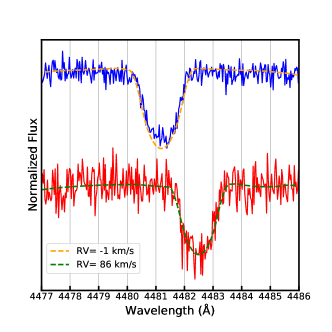
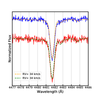
Figure 2: Observed Mg ii $4481.1\,\mathrm{\text{\AA}}$ absorption profiles (solid lines) for Gaia ID 3030259479295155072 (left) and Gaia ID 3030298374519750912 (right), with their best-fitting models (dashed lines). In both panels, the blue and red spectra represent the observations obtained in November 2020 and December 2021, respectively. The input RVs of the best-fitting models are listed in the legend.

Table 2: RV Measurement Results

Gaia IDa	$v\sin{i}$($\mathrm{km\,s^{-1}}$)b	$\mathrm{RV_{1}}$($\mathrm{km\,s^{-1}}$)c	$\mathrm{RV_{2}}$($\mathrm{km\,s^{-1}}$)c	$\mathrm{RV_{3}}$($\mathrm{km\,s^{-1}}$)c	$\mathrm{RV\ error}$($\mathrm{km\,s^{-1}}$)d	RV variation($\mathrm{km\,s^{-1}}$)	RV variation error($\mathrm{km\,s^{-1}}$)e	Obs numberf
3030259479295155072	$57\pm 1.7$	-1	85	86	$<2$	87	$<2.6$	3
3030027447983067008	$102\pm 2.9$	34	34	36	$<4$	2	$<4.0$	3
3028387801268979584	$40\pm 1.7$	43	54	39	$<2$	15	$<2.8$	3
3030231785345188608*	$88\pm 3.5$	33	36	–	$<3$	3	$<3.8$	2
3030030746517945600	$45\pm 1.7$	34	34	35	$<2$	1	$<2.0$	3
3030250751920573696*	$35\pm 1.7$	35	35	36	$<2$	1	$<2.0$	3
3029232707231846784	$100\pm 3.5$	33	33	–	$<3$	0	$<2.6$	2
3030038546178432256	$70\pm 2.1$	35	35	–	$<2$	0	$<1.7$	2
3030298374519750912*	$20\pm 1.7$	34	35	34	$<1$	1	$<1.2$	3
3030015215917673088	$30\pm 1.7$	34	36	32	$<2$	4	$<2.7$	3
3029919592765618304	$118\pm 2.9$	36	34	33	$<5$	3	$<5.1$	3
3030069263785446400	$30\pm 2.1$	37	31	–	$<1$	6	$<1.4$	2
3030313802042017536	$70\pm 1.7$	33	34	35	$<2$	2	$<2.3$	3
3030015662586533888	$37\pm 1.7$	34	34	34	$<2$	0	$<1.8$	3
3030026588989698048	$65\pm 1.7$	34	33	33	$<3$	1	$<2.9$	3
3030028684933623808*	$25\pm 3$	–	32	–	$<2$	–	–	1
3030016109262918016	$65\pm 2.1$	–	31	32	$<2$	1	$<2.0$	2
3030022152277677440*	$65\pm 2.1$	–	33	35	$<3$	2	$<3.3$	2
3030014013325413248	$80\pm 5$	–	34	–	$<2$	–	–	1
3030026138007337088	$85\pm 5$	–	33	–	$<4$	–	–	1
3030025661276778880	$25\pm 1.7$	36	36	37	$<2$	1	$<2.0$	3

• ID in Gaia EDR3;

• Measured mean $v\sin{i}$ values and their $2\sigma$ errors;

• $\mathrm{RV_{1}}$, $\mathrm{RV_{2}}$ and $\mathrm{RV_{3}}$ are the RVs observed in November 2020, November 2021 and December 2021, respectively, except for Gaia ID 3030025661276778880, for which data were obtained on 26 November 2021, 27 December 2021 and 28 December 2021, respectively;

• $2\sigma$ uncertainty of the RV measurement;

• $2\sigma$ uncertainty of the RV variations;

• Number of observations of the corresponding star;

• Stars classified as rMS stars by H22.

3 Main results

In Table 2, we present the measured RV values as well as the ranges of their $2\sigma$ uncertainties. The mean values of the measured $v\sin i$ for multiple observations for each star with their $2\sigma$ uncertainties are also listed. We confirm that the variations in the observed $v\sin i$ among multiple observations for each star are within the $v\sin i$ step ($5\,\mathrm{km\,s^{-1}}$) of our spectroscopic fits. We note that the measured $v\sin i$ of Gaia ID 302991959276561830 exceeds the upper limit of $v\sin i$ we adopted for selecting slowly rotating targets for RV measurements, based on H22. This may be caused by the different selection of absorption lines fitted in this paper compared with that of H22 for this particular target. Since its $v\sin i$ is close to the $v\sin i$ upper limit for selecting slowly rotating targets, we include this star in the discussion below.

The RV variations for each star, defined as the largest absolute difference among the RVs of a given star at different epochs, are also listed in Table 2. The number distributions of the RV variations of the 2-Obs and 3-Obs stars are plotted in Figure 3. To estimate the uncertainty in the RV variations, we generated 10,000 pseudo-RV values for each observed RV of every star based on the observed RV and its uncertainty, then obtained 10,000 RV variations for each star. Then, the uncertainty of the RV variations of a star is the standard deviation of its pseudo RV variations. In Table 2, we show the 2$\sigma$ uncertainty in the RV variations. Using this method, we also obtained 10,000 sets of pseudo RV variations for our targets. Based on the 10,000 sets of pseudo RV variations, we calculated the average number and the standard deviation of the number of stars in each RV variation bin, then derived an average distribution of RV variations for the 10,000 pseudo RV variation sets. The average distributions of the pseudo RV variation sets for different populations are shown in Figure 3. Using these average distributions, we determined the influence of the RV measurement errors on the distribution of observed RV variations.

Most (16 out of 18) 2-Obs stars show small RV variations $\leq 6\,\mathrm{km\,s^{-1}}$. Only two stars (Gaia ID 3028387801268979584 and 3030259479295155072) exhibit large RV variations $\geq 15\,\mathrm{km\,s^{-1}}$. Gaia ID 3028387801268979584, whose RV variation is $15\,\mathrm{km\,s^{-1}}$, shows a RV difference $\geq 10\,\mathrm{km\,s^{-1}}$ between subsequent observations. This star was found to be a double-lined spectroscopic binary system by H22. Gaia ID 3030259479295155072 exhibits the largest RV variation among our targets, $87\,\mathrm{km\,s^{-1}}$, between observations obtained in November 2020 and December 2021. We note that the RV difference for this star between the observations of November 2021 and December 2021 is as small as $1\,\mathrm{km\,s^{-1}}$. This may result from the similar orbital phases at the time that both observations were taken. We refer to these two stars which have RV variations $\geq 15\,\mathrm{km\,s^{-1}}$ as RV variable candidates. Their positions in the CMD are shown in Figure 1. The other 16 2-Obs stars and 10 3-Obs stars display relatively small RV variations ($\leq 6\,\mathrm{km\,s^{-1}}$) compared with those of the RV variable candidates. In the top-right inset of Figure 3, we plot the distribution of their RV variations and that of their RV variations plus $2\sigma$ uncertainties, which can be adopted as upper limits to their RV variations. Figure 3 shows that all upper limits to the RV variations are smaller than $10\,\mathrm{km\,s^{-1}}$. We refer to these 16 2-Obs stars and 10 3-Obs stars, whose upper limits to the RV variations $<10\,\mathrm{km\,s^{-1}}$, as our non-RV-variable candidates. They comprise 89 per cent (16/18) and 83 per cent (10/12) of the 2-Obs and 3-Obs stars, and 87 per cent (13/15) and 82 per cent (9/11) of the 2-Obs-shade and 3-Obs-shade stars, respectively. The fractions of the 2-Obs and 3-Obs stars showing RV variations $\leq 6\,\mathrm{km\,s^{-1}}$ are $82\pm 5$ per cent and $78\pm 6$ per cent in the sets of pseudo RV variations, respectively.

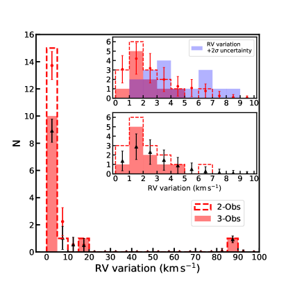
Figure 3: Number distributions of the measured RV variations of the 2-Obs (open and dashed symbols) and 3-Obs stars (filled symbols). The insets show the number distributions of the RV variations for the non-RV-variable candidates in these two populations, where the light blue bars in the top-right inset show the distribution of their RV variations plus their $2\sigma$ uncertainties (see Table 2). The error bar shows the average value and the standard deviation of the number in each RV variation bin for the 10,000 sets of pseudo RV variations (see the text), for the 2-Obs stars (red dots) and 3-Obs stars (black triangles).

In H22, we estimated the mean synchronisation time-scales, $\tau_{\mathrm{syn}}$, of 10 split-MS stars with $v\sin{i}<100\,\mathrm{km\,s^{-1}}$ using the theoretical equation (44) of Hurley et al. (2002). This equation is based on the dynamical tides theory proposed by Zahn (1975, 1977) . In H22, the correlation between $\tau_{\mathrm{syn}}$ and the fractional binary separation, $a/R$, was derived, where $a$ is the separation between the primary and the companion star and $R$ the radius of the primary star (see figure 12 of H22, ). In this work, we use $a$ and $R$ to represent the same quantities as in H22. In H22, we found that $\tau_{\mathrm{syn}}$ increased dramatically with increasing $a/R$. To fully tidally lock the binaries on time-scale on the order of the cluster age, a mean $a/R<4.5$ was required (H22). This indicates that large RV variations are expected in time-domain observations if our targets are close binaries which have been tidally locked on time-scales similar to the cluster age ($\sim 90\,\mathrm{Myr}$).

To compare the observed RV variations with those expected for binaries that have been fully or partially synchronised according to the dynamical tides theory, we modelled the RV variations when two- and three-epoch observations are taken for the 2-Obs and 3-Obs stars, respectively, using the $a/R$ range derived by H22. We first modelled assuming that their rotation rates were fully tidally braked within $90\,\mathrm{Myr}$, referring to the cases of two- and three-epoch observations as Case 2-Obs and Case 3-Obs, respectively. We assumed circularised orbits for the tidally locked binaries. As the observed RV of a star is the projection of its velocity along its orbit, the RV would be correlated with its $v\sin i$ instead of the equatorial rotation rate if the star were tidally locked. The radial velocity of the binary component, $\mathrm{RV_{obs}}$, of a tidally locked binary can thus be expressed as

$$\mathrm{RV_{obs}}=\mathrm{RV_{c}}+\frac{a}{R}v\sin{i}\frac{q}{1+q}\cos{\phi_{t}},$$ (1)

where $\mathrm{RV_{c}}$ is the centroid RV, $q$ the mass ratio of the primary to the companion and $\phi_{t}$ the phase of the binary orbit at the observation time, t. In our models, we adopted the average RV ($\sim 36\,\mathrm{km\,s^{-1}}$) of 57 NGC 2422 FGK-type stars measured by Bailey et al. (2018) as $\mathrm{RV_{c}}$. The input $v\sin i$ of the stars are their measured mean $v\sin i$, listed in Table 2. According to H22, the slowly rotating stars along the split MS of NGC 2422 should have intermediate mass ratios between 0.3 and 0.6 if they are photometric binaries. In each run, an intermediate $q$, uniformly distributed between 0.3 and 0.6, was thus applied for each star. High-mass-ratio close binaries may exhibit small RV variations because the shift in the absorption lines might be reduced owing to the comparable contribution of flux from both components. Since our targets have intermediate mass ratios if they are unresolved binaries, this effect would not be significant. The $a/R$ values adopted are uniformly distributed between 3 and 4.5 so as to synchronise the stellar rotation rates and the orbits of the slow rotators on time-scales shorter than the cluster age (H22). In each run of the Case 2-Obs and Case 3-Obs, every star was observed twice and three times, corresponding to two and three randomly generated $\phi_{t}$, uniformly distributed between 0 and $2\pi$, respectively. In each run, we also calculated the orbital periods, $T_{\mathrm{orb}}$, of the synthetic binaries using Kepler’s Third Law. Then the equatorial rotation rates of the primary stars, $v_{\mathrm{eq}}$, were estimated using $2\pi R/T_{\mathrm{orb}}$, where $R$ was estimated from the empirical relation $R\approx 1.33\times{M}^{0.555}$ for stars with $M>1.66\,\mathrm{M_{\odot}}$, where $M$ is given in units of $\mathrm{M_{\odot}}$ and $R$ in units of $\mathrm{R_{\odot}}$ (Demircan & Kahraman, 1991). We calculated $v\sin{i}/v_{\mathrm{eq}}$ for every star. For tidally locked binaries, $v\sin{i}/v_{\mathrm{eq}}$ should be smaller than unity. We repeated this procedure 10,000 times for each case and recorded the expected RV variations and $v\sin{i}/v_{\mathrm{eq}}$. For Case 2-Obs and Case 3-Obs, 70 per cent and 78 per cent, respectively, of the $v\sin{i}/v_{\mathrm{eq}}$ ratios in the 10,000 runs were less than unity. This implies that the set of $a$ and $q$ of most mock binaries were consistent with the assumption that they are tidally locked and show the measured $v\sin{i}$ values.

We additionally modelled binaries with $6\leq a/R\leq 8$ to explore the RV variations in case these stars are partially synchronised. This $a/R$ range corresponds to $\tau_{\mathrm{syn}}$ ranging from $\sim 1\,\mathrm{Gyr}$ to $\sim 10\,\mathrm{Gyr}$ ( H22, see their figure 12). Based on the models of D’Antona et al. (2017), stars whose rotation rates are reduced significantly but which are not tidally locked could also form a blue sequence. We refer to the models for $6\leq a/R\leq 8$ as Case 2-Obs-p and Case 3-Obs-p for our two- and three-epoch observations, respectively. Then the RV variations of stars whose rotation rates are reduced significantly but which are not tidally locked within $90\,\mathrm{Myr}$ should be located within the ranges of the Case 2-Obs (Case 3-Obs) and Case 2-Obs-p (Case 3-Obs-p) for the two-epoch (three-epoch) observations. For Case 2-Obs-p and Case 3-Obs-p, equation (1) cannot be used, since the periods of stellar rotation and the binary orbits are not synchronised. $\mathrm{RV_{obs}}$ is instead expressed as

$$\mathrm{RV_{obs}}=\mathrm{RV_{c}}+v_{\mathrm{orb}}\sin{j}\cos{\phi_{t}},$$ (2)

where $v_{\mathrm{orb}}$ is the velocity of the primary star along its binary orbit and $j$ is the inclination angle of the binary orbital rotation axis. Using Kepler’s Third Law, we calculated the orbital periods, $T_{\mathrm{orb}}$, for the mock binaries with $a/R$ uniformly distributed between 6 and 8, and $q$ uniformly distributed between 0.3 and 0.6, assuming circularised binary orbits. The $v_{\mathrm{orb}}$ values were then derived using $2\pi qa/(1+q)T_{\mathrm{orb}}$. The orientations of the orbital rotation axes were assumed to be stochastic in three-dimensional space, which was modelled using a uniform distribution of $\cos{j}$ between 0 and 1 (Lim et al., 2019). The set of $\phi_{t}$ values was the same for Case 2-Obs and Case 3-Obs. For each case, we repeated this process 10,000 times and recorded the synthetic RV variations. To test whether the synthetic binaries were indeed not tidally locked, we estimated their stellar rotation periods, $T_{\mathrm{rot}}$, using $2\pi R/v\sin{i}$ multiplied by a distribution of $\sin{i}$ generated like $\sin{j}$. In the 10,000 runs for Case 2-Obs-p and Case 3-Obs-p, 93 per cent and 90 per cent of the values of $T_{\mathrm{rot}}/T_{\mathrm{orb}}$ are less than unity, indicating that they are not tidally locked.

Figure 4 shows the density and cumulative distributions of the synthetic and observed RV variations for the Case 2-Obs, Case 3-Obs, Case 2-Obs-p and Case 3-Obs-p. In these four cases, it is evident that the synthetic RV variations exhibit much larger dispersions than the observations. For Case 2-Obs and Case 3-Obs, 82 and 96 per cent of the synthetic RV variations are larger than $10\,\mathrm{km\,s^{-1}}$, with mean synthetic RV variations of $55\,\mathrm{km\,s^{-1}}$ and $76\,\mathrm{km\,s^{-1}}$, respectively. For Case 2-Obs-p and Case 3-Obs-p, 78 and 95 per cent of synthetic RV variations are larger than $10\,\mathrm{km\,s^{-1}}$, with mean synthetic RV variations of $40\,\mathrm{km\,s^{-1}}$ and $61\,\mathrm{km\,s^{-1}}$, respectively. The synthetic results indicate a high probability, 82 per cent for Case 2-Obs, 96 per cent for Case 3-Obs, 78 per cent for Case 2-Obs-p and 95 per cent for Case 3-Obs-p, to detect RV variations $>10\,\mathrm{km\,s^{-1}}$ if the stars have corresponding fractional binary separations. Additionally, the chance to detect more stars with RV variation $\leq 10\,\mathrm{km\,s^{-1}}$ is small. For Case 2-Obs (Case 2-Obs-p), only 3 (17) out of the 10,000 runs have more than half of the stars showing RV variations $\leq 10\,\mathrm{km\,s^{-1}}$. Not a single run among the 10,000 runs for Case 3-Obs or Case 3-Obs-p has more than half of the stars showing RV variations $\leq 10\,\mathrm{km\,s^{-1}}$. However, our measurement results reveal that 89 per cent of 2-Obs and 83 per cent of 3-Obs stars are non-RV-variable candidates with RV variations $\leq 10\,\mathrm{km\,s^{-1}}$. For the 2-Obs-shade and 3-Obs-shade stars, the non-RV-variable candidates make up 87 and 82 per cent of their populations, respectively. In the 10,000 sets of pseudo RV variations, the fractions of the 2-Obs and 3-Obs stars showing RV variations $\leq 10\,\mathrm{km\,s^{-1}}$ are $89\pm 1$ per cent and $83\pm 2$ per cent, respectively. Only one star (Gaia ID 3030259479295155072) among the RV variable candidates which have three-epoch observations shows a comparable RV variation to the mean synthetic RV variations of the Case 3-Obs and the Case 3-Obs-p models. The distributions of the observed RV variations are different from those of the corresponding synthetic RV variations for the 2-Obs and 3-Obs stars. We applied Anderson–Darling tests for $k$ samples to explore whether the observed and synthetic RV variations are drawn from the same distribution. The tests for the four cases modelled all reported significance levels $p<0.001$, thus ruling out the hypothesis that the observed and synthetic RV variations come from the same distribution.

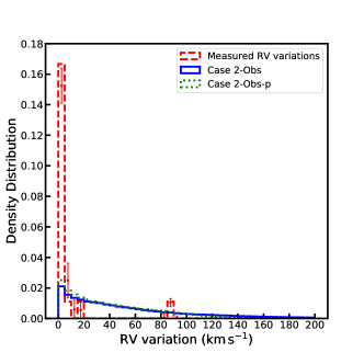
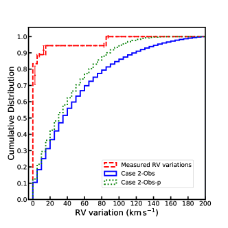
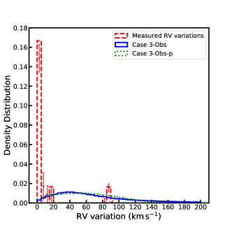
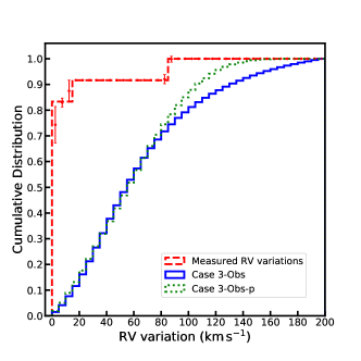
Figure 4: Density (left) and cumulative (right) distributions of the observed and synthetic RV variations. The observed RV variations are shown as red dashed lines in all panels. The two top panels show the distributions of the observed and synthetic RV variations for the 2-Obs stars. The synthetic RV variations for Case 2-Obs (Case 3-Obs) and Case 2-Obs-p (Case 3-Obs-p) are shown as the blue solid and green dotted lines in the two top (bottom) panels, respectively. The error bar shows the average value and the standard deviation of the number density (left) and the cumulative fraction (right) of the RV variations in each bin for the 10,000 sets of the pseudo RV variations of the 2-Obs stars (top two panels) and the 3-Obs stars (bottom two panels). The bin sizes in all panels are $5\,\mathrm{km\,s^{-1}}$

A large RV dispersion during a single epoch is expected if our targets are characterised by $a/R\leq 8$. In Figure 5, we show the synthetic RV dispersion at one epoch for the 21 spectroscopic targets assuming that they have been tidally locked within the cluster age, i.e., $3\leq a/R\leq 4.5$ (Case 1-Obs). The synthetic RV dispersion for $6\leq a/R\leq 8$ (Case 1-Obs-p) is also shown in Figure 5. In Case 1-Obs, the set of $\mathrm{RV_{c}}$, $v\sin i$, $a/R$ and $q$ are identical to those of Case 2-Obs or Case 3-Obs. For Case 1-Obs-p, the inputs of $\mathrm{RV_{c}}$, $v_{\mathrm{orb}}$ and $\sin{j}$ are the same as for Case 2-Obs-p or Case 3-Obs-p. $\phi_{t}$ was uniformly distributed between 0 and $2\pi$ in each run for all models. To present the RV dispersion, we subtracted the average $\mathrm{RV_{obs}}$ of the 21 stars from their $\mathrm{RV_{obs}}$ in each run. We repeated this process 10,000 times for each case. To compare with the observations, the dispersion in the observed RVs (RVs minus the mean RV) of the 21 stars on 26 and 27 November 2021, is plotted in Figure 5. The $1\sigma$ deviation of the observed RV dispersion is $11.6\,\mathrm{km\,s^{-1}}$; it would be $1.5\,\mathrm{km\,s^{-1}}$ if the two RV variable candidates are excluded. In fact, the average RV of the spectroscopic population excluding the RV-variable candidates is $33.8\,\mathrm{km\,s^{-1}}$ at this epoch. This is consistent with the mean RV ($\sim 36\,\mathrm{km\,s^{-1}}$) as for the 57 FGK-type cluster members in NGC 2422 reported by Bailey et al. (2018). The $1\sigma$ deviation for their RVs is $1.5\,\mathrm{km\,s^{-1}}$; the largest difference is $2.2\,\mathrm{km\,s^{-1}}$ between their RV values and their mean RV. We also generated 10,000 sets of pseudo RV dispersion for the 21 stars based on their measured RVs and the RV uncertainty. Their average distribution is plotted in Figure 4. This process was also repeated for the 21 stars excluding the RV-variable candidates. The mean value of the standard deviation of the 10,000 sets of their pseudo RV dispersion is $2.9\pm 0.5\,\mathrm{km\,s^{-1}}$. The dispersion in the measured RVs of the 21 stars, excluding the RV variable candidates, is much smaller than the synthetic RV dispersion, whose $1\sigma$ deviation is $53.3\,\mathrm{km\,s^{-1}}$ for Case 1-Obs or $35.7\,\mathrm{km\,s^{-1}}$ for Case 1-Obs-p. Anderson–Darling tests for the observed and synthetic RV dispersions of the 21 samples reported significance levels $p<0.001$ and $p=0.001$ for Case 1-Obs and Case 1-Obs-p, respectively, indicating that they are not drawn from the same distribution, in both cases.

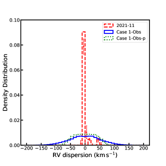
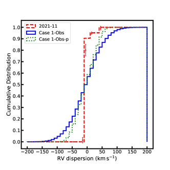
Figure 5: Density (left) and cumulative (right) distributions of the observed RV dispersion (red dashed line) on 26 and 27 November 2021, and the synthetic RV dispersion (blue solid lines) at a single epoch for the 21 targets. The error bar shows the average value and the standard deviation of the number density (left) and the cumulative fraction (right) of the RV dispersion in each bin for the 10,000 sets of the pseudo RV dispersion of the 21 targets. The bin sizes in all panels is $10\,\mathrm{km\,s^{-1}}$.

4 Discussion

In Section 3, we modelled the expected RV variations for binaries that were fully or partially synchronised within the cluster age, using the fractional separations derived based on the dynamical tides theory (Zahn, 1975, 1977; Hurley et al., 2002) in H22. The high fraction of stars with RV variations $\leq 10\,\mathrm{km\,s^{-1}}$ and the narrow dispersion of measured RVs at the single epoch indicate that most our spectroscopic targets are not in close binaries that can be tidally locked within the cluster age or even within $10\,\mathrm{Gyr}$. The non-RV-variable candidates comprise 87 per cent (13/15) of the 2-Obs-shade and 82 per cent (9/11) of the 3-Obs-shade stars. It is thus unlikely that tidal interactions dominate the formation of slowly rotating stars along the split MS. We emphasise that this result is based on a comparison with models characterised by the small $a/R$ ranges derived from the dynamical tides theory. In these models, the set of $a/R$ corresponds to $a$ separations between $0.02\,\mathrm{AU}$ and $0.10\,\mathrm{AU}$ and mean orbital periods of $1.38\pm 0.27\,\mathrm{days}$ (Case 2-Obs), $1.40\pm 0.28\,\mathrm{days}$ (Case 3-Obs), $3.52\pm 0.53\,\mathrm{days}$ (Case 2-Obs-p) and $3.57\pm 0.56\,\mathrm{days}$ (Case 3-Obs-p). The small binary separations give rise to large RV variations that are not consistent with the observed RV variation values.

However, Abt & Boonyarak (2004) uncovered a stronger effect of tidal interactions on stellar rotation than that predicted by the theory just described. Abt & Boonyarak (2004) explored the projected rotation rates and the orbital periods of 400 spectroscopic or visual binaries with B0 to F0 primary stars. The rotation rates of primary stars in binaries with $T_{\mathrm{orb}}$ of 4–500 days was also found to be substantially slowed down compared with that of single stars, presumably by tidal interactions (Abt & Boonyarak, 2004). This $T_{\mathrm{orb}}$ range was also proposed by D’Antona et al. (2015) as the possible orbital periods for slowly rotating split MS stars if their rotation is slowed down by tidal interactions. In Figure 6, we plot the correlations between the amplitudes of the projected orbital velocities (inclination angle $j=45\,\mathrm{{}^{\circ}}$) of the primary stars and the binary separations $a$ for different intermediate mass ratios $q$, assuming circularised binary orbits. The primary stars in Figure 6 have $1.8\,\mathrm{M_{\odot}}\leq M\leq 3.6\,\mathrm{M_{\odot}}$, which is similar to the mass range in the shaded region of Figure 1. In Figure 6, the $T_{\mathrm{orb}}$ of 100–$500\,\mathrm{days}$ correspond to $a$ of 0.6–$1.9\,\mathrm{AU}$, which is larger than the maximum $a$ adopted in the models by a factor of $\geq 6$. With this $a$ range, our targets may exhibit RV variations on the order of $1\,\mathrm{km\,s^{-1}}$.

We modeled the RV variations for a larger $a$ range than adopted for the models in Section 3. The models we ran were similar to Case 2-Obs-p and Case 3-Obs-p for the 2-Obs and 3-Obs stars, respectively, although the set of $\phi_{t}$ for the mock binaries with $T_{\mathrm{orb}}\geq 10\,\mathrm{days}$ was different. Their $\phi_{t}$ included a time interval of $365\,\mathrm{days}$ between the first and the second rounds, and a time interval of $30\,\mathrm{days}$ between the second and the third rounds, because their $T_{\mathrm{orb}}$ are comparable with the time intervals between the different observation epochs. We will refer to the fractions of the runs in which more than half of the stars show RV variations $\leq 10\,\mathrm{km\,s^{-1}}$ as $f_{\mathrm{half\leq 10}}$. In Figure 7, we plot the correlations of $f_{\mathrm{half\leq 10}}$ with the corresponding binary separations $a$. Based on Figure 7, we argue that the non-RV-variable candidates are not in close binaries with $a<0.2\,\mathrm{AU}$ ($T_{\mathrm{orb}}<19\,\mathrm{days}$), since $f_{\mathrm{half\leq 10}}$ is smaller than 5 per cent for this $a$ range. Additionally, most 3-Obs stars should have $a>0.6\,\mathrm{AU}$, corresponding to $T_{\mathrm{orb}}>\sim 100\,\mathrm{days}$. For binaries with $a$ of $0.6\sim 1.8\,\mathrm{AU}$ (grey shaded region), the probability that more than half show RV variations $\leq 10\,\mathrm{km\,s^{-1}}$ is greater than 0.05, corresponding to $T_{\mathrm{orb}}$ of 100–$500\,\mathrm{days}$. The fluctuations in $f_{\mathrm{half\leq 10}}$ across this $a$ range are caused by the comparable values of $T_{\mathrm{orb}}$ to the time intervals between the different rounds of our observations, leading to a greater possibility to detect small RV variations. We modelled the RV variations with $a$ uniformly distributed between $0.6\,\mathrm{AU}$ and $1.8\,\mathrm{AU}$. The result shows that $f_{\mathrm{half\leq 10}}$ is 86 per cent and 35 per cent for the mock two- and three-epoch observations, respectively. Based on the analysis for $f_{\mathrm{half\leq 10}}$, the possibility that our non-RV-variable candidates are binaries with $100\,\mathrm{days}<T_{\mathrm{orb}}<500\,\mathrm{days}$ cannot be excluded. With such long $T_{\mathrm{orb}}$, they may experience strong braking of stellar rotation owing to tidal interactions according to Abt & Boonyarak (2004). In Figure 8, we plot the distributions of the RV variations of the mock binaries with $100\,\mathrm{days}<T_{\mathrm{orb}}<500\,\mathrm{days}$ as well as those of the observed values for the 3-Obs stars. It seems that the observed RV variations are smaller than the synthetic RV variations. Eighty-two per cent of the 3-Obs stars have measured RV variations $\leq 5\,\mathrm{km\,s^{-1}}$ and they comprise all the non-RV-variable candidates in the 3-Obs stars. This fraction is $74\pm 7$ per cent in the sets of the pseudo RV variations where the RV measurement uncertainty are considered. However, the fraction of the synthetic RV variations $\leq 5\,\mathrm{km\,s^{-1}}$ is only 24 per cent for the 3-Obs stars. Nevertheless, because of the small number of the 3-Obs stars and the high possibility to detect RV variations on order of $1\,\mathrm{km\,s^{-1}}$ with such $T_{\mathrm{orb}}$ range, we suggest to explore the RV variability of slowly rotating massive stars in more clusters to confirm whether they are binary components with $T_{\mathrm{orb}}<500\,\mathrm{days}$.

Figure 6: Correlation of the orbital velocity, $v_{\mathrm{orb}}$, of the primary star, multiplied by $\sin{45^{\circ}}$, with the binary separation, $a$, for a mass range from $1.8\,\mathrm{M_{\odot}}$ to $3.6\,\mathrm{M_{\odot}}$. The blue dashed, green dotted and red solid lines show the correlations for $q=0.3$, $q=0.4$ and $q=0.6$, respectively. The correlations for $0.3<q<0.6$ are located within the grey shaded area. The error bars show the standard deviations associated with the different primary masses. The mean values of the orbital periods, in units of days, are colour-coded. The star labels along each line show the points corresponding to the mean orbital periods as indicated. The correlations were calculated based on Kepler’s Third Law, assuming circularised orbits.

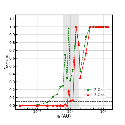
Figure 7: Fraction of runs in which more than half of the stars have RV variations $\leq 10\,\mathrm{km\,s^{-1}}$, $f_{\mathrm{half\leq 10}}$, versus binary separation, $a$. The results for the two- and three-epoch observations are shown using a green dashed line with star labels and a red solid line with triangular labels, respectively. The grey shaded area shows the range $0.6\,\mathrm{AU}<a<1.8\,\mathrm{AU}$, corresponding to $100\,\mathrm{days}<T_{\mathrm{orb}}<500\,\mathrm{days}$. The dotted horizontal line shows the locus for a fraction of 0.05.

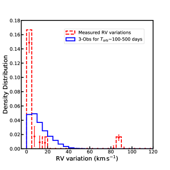
Figure 8: Density (left) and cumulative (right) distributions of the observed and synthetic RV variations for the 3-Obs stars if they have orbital periods of 100–500 days. The distributions of the observed and synthetic RV variations are shown as red dashed and blue solid lines, respectively. The error bar shows the average value and the standard deviation of the number density (left) and the cumulative fraction (right) of the RV variations in each bin for the 10,000 sets of the pseudo RV variations of the 3-Obs stars. The bin sizes in both panels are $5\,\mathrm{km\,s^{-1}}$

Our sample stars exhibiting small RV variations might be slowly rotating single stars or wide binary stars with $T_{\mathrm{orb}}>100\,\mathrm{days}$. According to Bastian et al. (2020), stars with close companions would disrupt their discs early on and tend to form rapidly rotating stars. Stars in wide binaries or single stars with long-surviving discs would form slow rotators, whose rotation is braked by disc locking (see also Zorec & Royer, 2012). Such systems would show RV varibility that is consistent with our observations. The correlation between wide binaries and slow rotators was implied by Yang et al. (2021), who found that the spatial distributions of bMS stars were more like those of soft binaries. The binary-merger scenario suggested by Wang et al. (2022) would naturally produce slowly rotating single stars. These two scenarios need more observational confirmation, however. For example, Bastian et al. (2020) proposed to explore the distribution of the rotation rates of early-type stars in very young (a few Myr-old) clusters to test whether they are bimodal. Wang et al. (2022) suggested to study the slope of the mass functions of field stars or the evolution of the stellar mass functions in star clusters, since stellar mass functions may vary owing to binary mergers.

In H22, we detected a weak correlation between stellar colours and rotation rates among the split-MS stars of NGC 2422, casting some doubt on their relationship. This correlation is caused by the appearance of a large fraction of rMS stars with small $v\sin i$ similar to the bMS stars. In H22, we interpreted these slowly rotating rMS stars as photometric binaries. Their loci in the CMD are shifted to the redder and brighter side, rendering them close to the rMS owing to contamination by hidden low-mass companions. This explanation cannot be ruled out. Based on Gaia Collaboration et al. (2021), the completeness of close source pairs drops significantly for separations below about $0.7\,\mathrm{arcsec}$. This angular separation corresponds to $\sim 333\,\mathrm{AU}$ at the distance of NGC 2422, which is much wider than the separations of the sample binaries discussed above. The slowly rotating rMS stars might be unresolved binaries with $0.6\,\mathrm{AU}<a<333\,\mathrm{AU}$. Then, the four spectroscopic targets in this papers classified as rMS stars by H22 with multiple observations (see Table 2) could be unresolved binaries and show small RV variations ($\leq 3\,\mathrm{km\,s^{-1}}$).

However, the possibility that the small $v\sin{i}$ values of the rMS stars are caused by small inclination angles $i$ of the rotation axis cannot be ruled out. In Figure 9, we show two coeval synthetic populations derived from the SYCLIST database (Georgy et al., 2013, 2014), with one population that does not rotate whereas the other is rotating at 90 per cent of the critical rotation rate ($\mathrm{\omega_{crit}}$). The synthetic populations are $\sim 90\,\mathrm{Myr}$ old, with $Z=Z_{\odot}$. The inclination angles of both populations are randomly distributed; the $i$ angles of the rapidly rotating stars are colour-coded in units of degrees. Only single stars are included in the synthetic populations. The gravity darkening law from Espinosa Lara & Rieutord (2011) and the limb-darkening law from Claret (2000) have been implemented. The synthetic absolute magnitudes are calculated based on Evans et al. (2018) for Gaia Data Release 2. The grey shaded area in Figure 9 shows the region that covers the mass range of $1.8\,\mathrm{M_{\odot}}<M<3.6\,\mathrm{M_{\odot}}$, which is similar to the shaded region in Figure 1 that represents the loci where the split pattern is evident. The effect of varying $i$ on the morphology of the rapidly rotating population is significant in the region close to the MSTO, while it does not extend the full width of the rMS.

Gravity darkening caused by stellar rotation makes the poles hotter than the equators at the surface of rapidly rotating stars. The contrast of the effective temperature between the poles and equators could be enhanced by the limb-darkening effect (Georgy et al., 2014). This results in a scenario where rapidly rotating stars observed pole-on appear hotter and brighter than their counterparts which are observed equator-on (Georgy et al., 2014), i.e., they will be bluer and brighter in the CMDs of star clusters. The direction of this shift seems to align with the distribution of the rMS (see the rapidly rotating populations for different $i$ and the shift of a star for different $i$ in Figure 9), making rapidly rotating stars with small $i$, which correspond to small $v\sin i$, appear on the rMS alongside their counterparts with large $i$. In Figure 10, we also plot the distributions of synthetic populations with older ages ($150\,\mathrm{Myr}$ and $200\,\mathrm{Myr}$), where we find a similar phenomenon, i.e., that rapid rotators with different $i$ are located along the rMSs. The physics that causes this phenomenon is unclear. It might be linked to the correlation of effective temperature with luminosity at the surface towards the observer at different inclination angles, or to the profiles of the colours and magnitudes observed through Gaia passbands. The rMS stars with small $v\sin i$ observed in NGC 2422 might thus be some rapidly rotating single stars showing their poles, which breaks the $v\sin{i}$–colour correlation expected for the upper MS stars in young star clusters.

Figure 9: Synthetic coeval populations with different stellar rotation rates derived from the SYCLIST database (Georgy et al., 2013, 2014). The blue crosses show the non-rotating population. The dots show the rapidly rotating population at $0.9\mathrm{\omega_{crit}}$, colour-coded by the inclination angles of the stellar rotation axes, in units of degrees. The dashed circles show the loci of two stars with the same mass ($1.72\,\mathrm{M_{\odot}}$) but different inclination angles, $i$. The arrow represents the shift in colour and magnitude from $i=89\,\mathrm{{}^{\circ}}$ to $i=19\,\mathrm{{}^{\circ}}$. The grey shading covers the mass range of $1.8\,\mathrm{M_{\odot}}<M<3.6\,\mathrm{M_{\odot}}$.

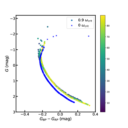
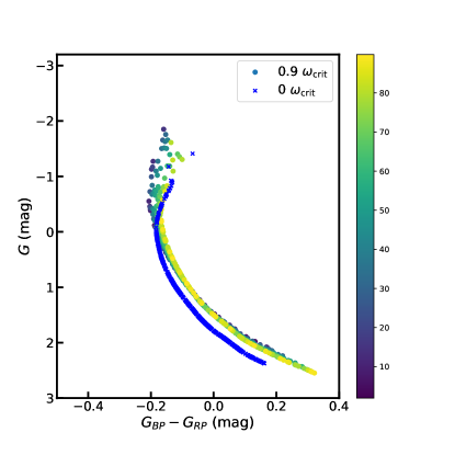
Figure 10: As Figure 9, but for synthetic populations with ages of $150\,\mathrm{Myr}$ (left) and $200\,\mathrm{Myr}$ (right).

5 Conclusion

Using high-resolution spectra observed with the CFHT at multiple epochs, we explored the RV variability of 21 slowly rotating stars ($v\sin{i}\leq 104\,\mathrm{km\,s^{-1}}$) along the split MS of NGC 2422 ($90\,\mathrm{Myr}$). We found that (1) most our targets exhibit RV variations that are much smaller than those expected for binaries that are tidally locked within the cluster age (Case 2-Obs and Case 3-Obs) or within $10\,\mathrm{Gyr}$ (Case 2-Obs-p and Case 3-Obs-p); (2) The dispersion of the measured RVs at a single epoch is much smaller than that for synthetic binaries that become tidally locked within the cluster age (Case 1-Obs) or within $10\,\mathrm{Gyr}$ (Case 1-Obs-p). We thus conclude that most of our targets are not close binaries whose stellar rotation rates can be tidally reduced substantially on time-scales shorter than the cluster age, that is, tidal interactions are not dominant in the formation of slowly rotating stars along the split MSs of young star clusters. However, we emphasise that this result is based on theoretical predictions for binary separations to partially or fully synchronise the stars in H22 using equation (44) of Hurley et al. (2002), which is based on the dynamical tides theory of Zahn (1975, 1977). Observations by Abt & Boonyarak (2004) show a stronger effect of tidal interactions on stellar rotation than the predictions from the above theory on shorter times-scales or larger binary separations. The latter authors found that the rotation rates of the primary B0–F0-type stars in binaries with $T_{\mathrm{orb}}$ of 4–500 days are also substantially slowed down compared with those of single stars. If our targets are in binaries with $100\,\mathrm{days}<T_{\mathrm{orb}}<500\,\mathrm{days}$, they may show small RV variations like those observed. Based on Abt & Boonyarak (2004), the stellar rotation rates in such systems can be reduced significantly by tidal interactions.

The slow rotators along the split MS could be single stars or wide binaries whose separations are larger than $\sim 0.6\,\mathrm{AU}$ ($T_{\mathrm{orb}}>\sim 100\,\mathrm{days}$). This kind of binary systems could show small RV variations like those of most our targets in time-domain observations. In H22, we detected a large fraction of rMS stars showing similar $v\sin i$ to those of the bMS stars. They might be photometric binaries with separations larger than $\sim 0.6\,\mathrm{AU}$ and smaller than $\sim 333\,\mathrm{AU}$. The photometry of rapidly rotating single stars with small inclination angles could also account for the rMS stars that exhibit small projected rotation rates.

Data Availability

The public data used in our analysis is accessible through the following links:

• Gaia EDR3 (Gaia Collaboration et al., 2016, 2021): https://gea.esac.esa.int/archive/

• PARSEC Isochrones (Marigo et al., 2017): http://stev.oapd.inaf.it/cgi-bin/cmd

• SYCLIST Database (Georgy et al., 2013, 2014): https://www.unige.ch/sciences/astro/evolution/en/database/

The spectroscopic data used in this paper can be shared based on reasonable request to the corresponding author.

References

- Abt & Boonyarak (2004) Abt H. A., Boonyarak C., 2004, ApJ, 616, 562
- Bailey et al. (2018) Bailey J. I., Mateo M., White R. J., Shectman S. A., Crane J. D., 2018, MNRAS, 475, 1609
- Bastian & Niederhofer (2015) Bastian N., Niederhofer F., 2015, MNRAS, 448, 1863
- Bastian & Strader (2014) Bastian N., Strader J., 2014, MNRAS, 443, 3594
- Bastian & de Mink (2009) Bastian N., de Mink S. E., 2009, MNRAS, 398, L11
- Bastian et al. (2020) Bastian N., Kamann S., Amard L., Charbonnel C., Haemmerlé L., Matt S. P., 2020, MNRAS, 495, 1978
- Claret (2000) Claret A., 2000, A&A, 363, 1081
- Cordoni et al. (2018) Cordoni G., Milone A. P., Marino A. F., Di Criscienzo M., D’Antona F., Dotter A., Lagioia E. P., Tailo M., 2018, ApJ, 869, 139
- Correnti et al. (2017) Correnti M., Goudfrooij P., Bellini A., Kalirai J. S., Puzia T. H., 2017, MNRAS, 467, 3628
- Czesla et al. (2019) Czesla S., Schröter S., Schneider C. P., Huber K. F., Pfeifer F., Andreasen D. T., Zechmeister M., 2019, PyA: Python astronomy-related packages (ascl:1906.010)
- D’Antona et al. (2015) D’Antona F., Di Criscienzo M., Decressin T., Milone A. P., Vesperini E., Ventura P., 2015, MNRAS, 453, 2637
- D’Antona et al. (2017) D’Antona F., Milone A. P., Tailo M., Ventura P., Vesperini E., di Criscienzo M., 2017, Nature Astronomy, 1, 0186
- Demircan & Kahraman (1991) Demircan O., Kahraman G., 1991, Ap&SS, 181, 313
- Dufton et al. (2013) Dufton P. L., et al., 2013, A&A, 550, A109
- Dupree et al. (2017) Dupree A. K., et al., 2017, ApJ, 846, L1
- Espinosa Lara & Rieutord (2011) Espinosa Lara F., Rieutord M., 2011, A&A, 533, A43
- Evans et al. (2018) Evans D. W., et al., 2018, A&A, 616, A4
- Gaia Collaboration et al. (2016) Gaia Collaboration et al., 2016, A&A, 595, A1
- Gaia Collaboration et al. (2021) Gaia Collaboration et al., 2021, A&A, 649, A1
- Georgy et al. (2013) Georgy C., Ekström S., Granada A., Meynet G., Mowlavi N., Eggenberger P., Maeder A., 2013, A&A, 553, A24
- Georgy et al. (2014) Georgy C., Granada A., Ekström S., Meynet G., Anderson R. I., Wyttenbach A., Eggenberger P., Maeder A., 2014, A&A, 566, A21
- Goudfrooij et al. (2009) Goudfrooij P., Puzia T. H., Kozhurina-Platais V., Chandar R., 2009, AJ, 137, 4988
- Goudfrooij et al. (2011) Goudfrooij P., Puzia T. H., Chandar R., Kozhurina-Platais V., 2011, ApJ, 737, 4
- Goudfrooij et al. (2017) Goudfrooij P., Girardi L., Correnti M., 2017, ApJ, 846, 22
- He et al. (2022) He C., et al., 2022, ApJ, 938, 42
- He et al. (2023) He C., et al., 2023, ApJ, 952, 172
- Hubeny & Lanz (1992) Hubeny I., Lanz T., 1992, A&A, 262, 501
- Hurley et al. (2002) Hurley J. R., Tout C. A., Pols O. R., 2002, MNRAS, 329, 897
- Kamann et al. (2020) Kamann S., et al., 2020, MNRAS, 492, 2177
- Kamann et al. (2021) Kamann S., Bastian N., Usher C., Cabrera-Ziri I., Saracino S., 2021, MNRAS, 508, 2302
- Kamann et al. (2023) Kamann S., et al., 2023, MNRAS, 518, 1505
- Kraft (1967) Kraft R. P., 1967, ApJ, 150, 551
- Kurucz (2005a) Kurucz R. L., 2005a, Memorie della Societa Astronomica Italiana Supplementi, 8, 86
- Kurucz (2005b) Kurucz R. L., 2005b, Memorie della Societa Astronomica Italiana Supplementi, 8, 189
- Kurucz (2011) Kurucz R. L., 2011, Canadian Journal of Physics, 89, 417
- Kurucz (2018) Kurucz R. L., 2018, in Workshop on Astrophysical Opacities. p. 47
- Li et al. (2014a) Li C., de Grijs R., Deng L., 2014a, Nature, 516, 367
- Li et al. (2014b) Li C., de Grijs R., Deng L., 2014b, ApJ, 784, 157
- Li et al. (2016) Li C., de Grijs R., Bastian N., Deng L., Niederhofer F., Zhang C., 2016, MNRAS, 461, 3212
- Li et al. (2017) Li C., de Grijs R., Deng L., Milone A. P., 2017, ApJ, 844, 119
- Li et al. (2019) Li C., Sun W., de Grijs R., Deng L., Wang K., Cordoni G., Milone A. P., 2019, ApJ, 876, 65
- Lim et al. (2019) Lim B., Rauw G., Nazé Y., Sung H., Hwang N., Park B.-G., 2019, Nature Astronomy, 3, 76
- Mackey et al. (2008) Mackey A. D., Broby Nielsen P., Ferguson A. M. N., Richardson J. C., 2008, ApJ, 681, L17
- Marigo et al. (2017) Marigo P., et al., 2017, ApJ, 835, 77
- Marino et al. (2018a) Marino A. F., Przybilla N., Milone A. P., Da Costa G., D’Antona F., Dotter A., Dupree A., 2018a, AJ, 156, 116
- Marino et al. (2018b) Marino A. F., Milone A. P., Casagrande L., Przybilla N., Balaguer-Núñez L., Di Criscienzo M., Serenelli A., Vilardell F., 2018b, ApJ, 863, L33
- McLaughlin & van der Marel (2005) McLaughlin D. E., van der Marel R. P., 2005, ApJS, 161, 304
- Milone et al. (2009) Milone A. P., Bedin L. R., Piotto G., Anderson J., 2009, A&A, 497, 755
- Milone et al. (2016) Milone A. P., Marino A. F., D’Antona F., Bedin L. R., Da Costa G. S., Jerjen H., Mackey A. D., 2016, MNRAS, 458, 4368
- Milone et al. (2017) Milone A. P., et al., 2017, MNRAS, 465, 4363
- Milone et al. (2018) Milone A. P., et al., 2018, MNRAS, 477, 2640
- Palacios et al. (2010) Palacios A., Gebran M., Josselin E., Martins F., Plez B., Belmas M., Lèbre A., 2010, A&A, 516, A13
- STScI Development Team (2013) STScI Development Team 2013, pysynphot: Synthetic photometry software package, Astrophysics Source Code Library, record ascl:1303.023 (ascl:1303.023)
- Schneider et al. (2019) Schneider F. R. N., Ohlmann S. T., Podsiadlowski P., Röpke F. K., Balbus S. A., Pakmor R., Springel V., 2019, Nature, 574, 211
- Sun et al. (2019a) Sun W., de Grijs R., Deng L., Albrow M. D., 2019a, ApJ, 876, 113
- Sun et al. (2019b) Sun W., Li C., Deng L., de Grijs R., 2019b, ApJ, 883, 182
- Sun et al. (2021) Sun W., Duan X.-W., Deng L., de Grijs R., 2021, ApJ, 921, 145
- Wang et al. (2022) Wang C., et al., 2022, Nature Astronomy, 6, 480
- Wang et al. (2023) Wang L., Li C., Wang L., He C., Wang C., 2023, The Astrophysical Journal, 949, 53
- Yang et al. (2021) Yang Y., Li C., de Grijs R., Deng L., 2021, ApJ, 912, 27
- Yang et al. (2022) Yang Y., Li C., Huang Y., Liu X., 2022, ApJ, 925, 159
- Zahn (1975) Zahn J. P., 1975, A&A, 41, 329
- Zahn (1977) Zahn J. P., 1977, A&A, 57, 383
- Zorec & Royer (2012) Zorec J., Royer F., 2012, A&A, 537, A120