Charged Anisotropic Tolman IV Solution in Matter-Geometry Coupled Theory

Abstract

This paper discusses the interior distribution of several anisotropic star models coupled with an electromagnetic field in the context of $f(\mathcal{R},\mathcal{T},\mathcal{Q})$ gravity, where $\mathcal{Q}=\mathcal{R}_{\beta\xi}\mathcal{T}^{\beta\xi}$. In this regard, a standard model of this modified gravity is taken as $\mathcal{R}+\nu_{3}\mathcal{R}_{\beta\xi}\mathcal{T}^{\beta\xi}$, where $\nu_{3}$ symbolizes an arbitrary coupling constant. We assume a charged spherically symmetric metric that represents the interior geometry of compact quark stars and develop the corresponding modified field equations. These equations are then solved with the help of metric potentials of Tolman IV spacetime and a linear bag model equation of state. We consider the experimental data (i.e., radii and masses) of different quark models such as SMC X-4, SAX J 1808.4-3658, Her X-I and 4U 1820-30 to analyze how the charge and modified corrections affect their physical characteristics. The viability and stability of the resulting model is also checked for the considered star candidates with two different values of $\nu_{3}$. We conclude that only two models, Her X-I and 4U 1820-30 show stable behavior in this modified framework for both values of the coupling constant.

Keywords: $f(\mathcal{R},\mathcal{T},\mathcal{R}_{\beta\xi}\mathcal{T}^{\beta\xi})$ theory; Compact stars; Stability.
PACS: 04.50.Kd; 04.40.Dg; 04.40.-b.

1 Introduction

A widely accepted theory of gravitation is considered as general relativity ($\mathbb{GR}$) that addresses various challenges related to cosmic evolution. However, it is still not sufficiently enough to explain an accelerated expansion of the universe properly. In view of this, various modifications to $\mathbb{GR}$ have been proposed that were claimed to handle mystifying issues (i.e., the dark matter and expeditious expanding cosmos etc.) in some better way. It was pointed out by several astrophysical experiments that there exists a heavy amount of a mysterious force having large negative pressure, and thus causes such accelerated expansion, called dark energy. The first ever extension to $\mathbb{GR}$ has been proposed by modifying the geometric part of the Einstein-Hilbert action in which the Ricci scalar $\mathcal{R}$ was swapped by its generic function, thus termed the $f(\mathcal{R})$ gravity [1]. Multiple models of this modified theory have been discussed in the literature and it was deduced that they produce viable and stable self-gravitating models [2]-[5].

An interesting notion in the framework of $f(\mathcal{R})$ gravity was initially introduced by Bertolami et al. [6], in which they coupled the effects of matter and geometric terms in the matter Lagrangian. This idea prompted many scientists to study how such a coupling affects the interior of a self-gravitating object. The interesting results were found after an extensive study that urged researchers to generalize the concept of coupling at the action level. This has been done by Harko et al. [7] for the first time, who introduced $f(\mathcal{R},\mathcal{T})$ gravitational theory, in which $\mathcal{T}$ indicates trace of the energy-momentum tensor $(\mathbb{EMT})$. However, such a generalized coupling immediately makes this modified theory non-conserved, opposing $f(\mathcal{R})$ gravity as well as $\mathbb{GR}$. Several impressive astrophysical outcomes have been observed while studying this extended theory [8]-[13].

The $f(\mathcal{R},\mathcal{T})$ gravity was further extended by Haghani et al. [14] who added a term $\mathcal{Q}\equiv\mathcal{R}_{\beta\xi}\mathcal{T}^{\beta\xi}$ in the preceding functional. The viability of three distinct models have been studied thoroughly in this framework. The main reason to suggest this theory is that the $f(\mathcal{R},\mathcal{T})$ gravity fails to entail a non-minimal interaction on test particles when a traceless fluid distribution is assumed. However, this theory does entail even in this scenario due to the term $\mathcal{R}_{\beta\xi}\mathcal{T}^{\beta\xi}$. The galactic rotation and exponential expansion era of our universe can also be studied with the help of this theory. Sharif and Zubair [15] chosen density as well as pressure-dependent matter Lagrangian, and discussed the laws of black hole thermodynamics for the models such as $\mathcal{R}+\nu_{3}\mathcal{R}_{\beta\xi}\mathcal{T}^{\beta\xi}$ and $\mathcal{R}(1+\nu_{3}\mathcal{R}_{\beta\xi}\mathcal{T}^{\beta\xi})$. The physical viability of these two models has also been checked and it was deduced that negative coupling constant does not satisfy the weak energy bounds [16].

The modified cosmological solutions have been formulated by Odintsov and Sáez-Gómez [17], and they also verified that the $\Lambda$CDM model is supported by this extended gravity. Baffou et al. [18] explored the stable regions of the solutions (obtained by solving Friedmann equations numerically) with respect to two different $f(\mathcal{R},\mathcal{T},\mathcal{Q})$ models. Sharif and Waseem [19, 20] discussed the isotropic/anisotropic structures by taking the matter Lagrangian to be the negative pressure in this theory and obtained unaccepted physical results. Yousaf and his collaborators [21]-[26] split the Riemann tensor (engaging modified $\mathbb{EMT}$) to obtain some scalars which are used to study the interior configuration of self-gravitating spherical systems. The simplest possible evolutionary modes along with the complexity factor for non-static cylindrical systems have also been studied [27, 28]. Recently, we have used the decoupling approach and a quark model equation of state to obtain feasible solutions of modified field equations [29]-[31].

Researchers have done extensive analysis in the scenario of $\mathbb{GR}$ and modified theories of gravity to check whether the presence of charge in the interior of a compact star makes it physically more relevant or not. An exterior geometry represented by the Reissner-Nordström metric has been considered by Das et al. [32], with the help of which they calculated the solution of a charged model at the spherical interface. Sunzu et al. [33] employed a well-known relation between radius and mass of a strange quark star whose interior was influenced from an electromagnetic field, and discussed its physical properties. An extensive analysis has been done on the physical relevancy of charged compact self-gravitating objects, and it was deduced that the presence of charge makes these systems more stable [34]-[41].

Neutron stars have such intense gravity that they crush electrons and protons together into neutrons. The whole star is made of neutrons, inside and out. If more mass is added to the neutron star, it will be impossible to hold even the neutrons together, and the whole object collapses into a black hole. An in-between stage of neutron stars and black holes is the quark star that has too much mass in its center for the neutrons to hold their atomness, however, not enough to completely collapse into a black hole. Quarks are considered as elementary particles that come in six different types such as up, down, top, bottom, charm and strange. The two flavors namely ‘up’ and ‘down’ quarks are squeezed together into ‘strange’ quarks. Since it is composed of ‘strange’ quarks, physicists name this ‘strange matter’. The conjecture that strange matter may be the absolute ground state of strongly interacting matter resulted in the possible existence of strange stars [42, 43]. It has been shown in recent studies that the compact objects associated with the x-ray pulsar such as Her X-I and 4U 1820-30 are good candidates for strange stars [44, 45]. Moreover, the charge has been estimated inside several quark candidates and found to be within the interval $(1.5453\times 10^{18}C,7.6271\times 10^{19}C)$ [46]. It was also deduced that minimum and maximum charge corresponds to the stars Her X-I and SMC X-I, respectively.

Some constraints have been introduced in the literature that interlink different physical variables representing isotropic/anisotropic interiors such as pressure and energy density. Among such constraints, one is the $\mathbf{MIT}$ bag model equation of state ($\mathbf{E}$o$\mathbf{S}$) that portrays the quark’ interior [32]. It was observed that only this $\mathbf{E}$o$\mathbf{S}$ is feasible to calculate the compactness of strange quark systems like Her X-1, RXJ 185635-3754, 4U 1728-34, 4U 1820-30, PSR 0943+10 and SAX J 1808.4-3658, etc. because an $\mathbf{E}$o$\mathbf{S}$ for neutron stars flunk to do so [47]. The bag constant involving in $\mathbf{MIT}$ $\mathbf{E}$o$\mathbf{S}$ helps to determine the difference between the true and the false state of a vacuum. An interior fluid configuration of quark bodies has been extensively studied with the help of this model [48]-[50]. Demorest et al. [51] considered a strange star PSR J1614-2230 and discussed its several fundamental characteristics. They found $\mathbf{MIT}$ bag model to be the only suitable candidate to discuss a family of such heavy objects. Rahaman et al. [52] adopted the same model and explored mass as well as other physical properties of compact systems through interpolating technique.

Various approaches have been employed to develop solution to the highly complicated field equations in any theory of gravitation (either $\mathbb{GR}$ or modified gravity). For instance, a specific $\mathbf{E}$o$\mathbf{S}$ or developed forms of the metric functions, etc. can be used in order to do this. One of these well-known metric potentials is the Tolman IV spacetime that has been adopted by various researchers to obtain physically acceptable compact models in different theories of gravity. Murad and Fatema [53] developed some anisotropic models by using this solution and showed their physical relevancy through graphical analysis. Bhar et al. [54] investigated physical characteristics corresponding to various compact structures by using Tolman IV spacetime and found their resulting solution to be singularity-free and viable. Malaver [55] adopted the same solution and developed a physically feasible charged model to check how an electromagnetic field affects it. This spacetime has also been coupled with the complexity factor of anisotropic fluid distribution through which an acceptable compact model is developed in the context of $\mathbb{GR}$ as well as Brans-Dicke theory [56, 57]. A charged realistic isotropic solution was formulated and graphically interpreted with respect to some particular stars such as SAX J1808.4-3658, Her X-1 and 4U 1538-52 [58].

In this article, we discuss the interior fluid configuration of the charged anisotropic quark stars in modified $f(\mathcal{R},\mathcal{T},\mathcal{Q})$ theory of gravity. The format of this paper is given as follows. Section 2 defines some fundamental entities of this modified gravity and establishes the field equations for a specific model given by $\mathcal{R}+\nu_{3}\mathcal{R}_{\beta\xi}\mathcal{T}^{\beta\xi}$. We then use the metric components of Tolman IV spacetime and $\mathbf{MIT}$ bag model $\mathbf{E}$o$\mathbf{S}$ to solve the field equations. Section 3 calculates the unknown constants with the help of the boundary conditions. We further explore the effects of this theory and charge on matter determinants and stability of compact models in section 4. Finally, section 5 summarizes all our results.

2 Modified Theory

The action corresponding to $f(\mathcal{R},\mathcal{T},\mathcal{Q})$ gravitational theory (with $\kappa=8\pi$) is given by [17]

$$\mathbb{I}=\int\sqrt{-g}\left\{\frac{f(\mathcal{R},\mathcal{T},\mathcal{Q})}{16\pi}+\mathbf{L}_{\mathrm{E}}+\mathbf{L}_{m}\right\}d^{4}x,$$ (1)

where $\mathbf{L}_{\mathrm{E}}$ and $\mathbf{L}_{m}$ being the Lagrangian densities of the electromagnetic field and fluid distribution, respectively. The principle of least-action provides after implementing on Eq.(1) as

$$\mathcal{G}_{\beta\xi}=\mathcal{T}_{\beta\xi}^{(\mathrm{ef})}=8\pi\bigg{\{}\frac{1}{f_{\mathcal{R}}-\mathbf{L}_{m}f_{\mathcal{Q}}}\left(\mathcal{T}_{\beta\xi}+\mathrm{E}_{\beta\xi}\right)+\mathcal{T}_{\beta\xi}^{(\mathrm{cr})}\bigg{\}},$$ (2)

where the Einstein tensor $\mathcal{G}_{\beta\xi}$ represents the spacetime geometry and $\mathcal{T}_{\beta\xi}^{(\mathrm{ef})}$ is the total $\mathbb{EMT}$ of this extended theory. Also, $\mathcal{T}_{\beta\xi}$ and $\mathrm{E}_{\beta\xi}$ are the usual $\mathbb{EMT}$ and the electromagnetic tensor, respectively. The last term $\mathcal{T}_{\beta\xi}^{(\mathrm{cr})}$ of the above equation takes the following form

$$\mathcal{T}_{\beta\xi}^{(\mathrm{cr})} = -\frac{1}{8\pi\bigg{(}\mathbf{L}_{m}f_{\mathcal{Q}}-f_{\mathcal{R}}\bigg{)}}\left[\left(f_{\mathcal{T}}+\frac{1}{2}\mathcal{R}f_{\mathcal{Q}}\right)\mathcal{T}_{\beta\xi}+\left\{\frac{\mathcal{R}}{2}(\frac{f}{\mathcal{R}}-f_{\mathcal{R}})-\mathbf{L}_{m}f_{\mathcal{T}}\right.\right.$$ (3)

$$- \left.\frac{1}{2}\nabla_{\eta}\nabla_{\lambda}(f_{\mathcal{Q}}\mathcal{T}^{\eta\lambda})\right\}g_{\beta\xi}-\frac{1}{2}\Box(f_{\mathcal{Q}}\mathcal{T}_{\beta\xi})-(g_{\beta\xi}\Box-\nabla_{\beta}\nabla_{\xi})f_{\mathcal{R}}$$

$$- 2f_{\mathcal{Q}}\mathcal{R}_{\eta(\beta}\mathcal{T}_{\xi)}^{\eta}+\nabla_{\eta}\nabla_{(\beta}[\mathcal{T}_{\xi)}^{\eta}f_{\mathcal{Q}}]+2(f_{\mathcal{Q}}\mathcal{R}^{\eta\lambda}+\left.f_{\mathcal{T}}g^{\eta\lambda})\frac{\partial^{2}\mathbf{L}_{m}}{\partial g^{\beta\xi}\partial g^{\eta\lambda}}\right].$$

Here, $f=f({\mathcal{R}},{\mathcal{T}},{\mathcal{Q}})$ is partially differentiated with respect to its arguments and represented by $f_{\mathcal{R}},~{}f_{\mathcal{T}}$ and $f_{\mathcal{Q}}$. Also, the D’Alambert operator is defined as $\Box\equiv\frac{1}{\sqrt{-g}}\partial_{\beta}\big{(}\sqrt{-g}g^{\beta\xi}\partial_{\xi}\big{)}$ and $\nabla_{\beta}$ is the covariant derivative.

We recall that the expression of the matter Lagrangian density is not unique, rather this depends on nature of the matter source of the universe [14]. Usually, it can be taken in terms of the energy density, pressure or some scalar field. Since we consider the charged framework, a more appropriate choice of the matter Lagrangian in this regard is taken as $\mathbf{L}_{m}=-\frac{1}{4}\mathcal{Z}_{\beta\xi}\mathcal{Z}^{\beta\xi}$, giving rise to $\frac{\partial^{2}\mathbf{L}_{m}}{\partial g^{\beta\xi}\partial g^{\eta\lambda}}=-\frac{1}{2}\mathcal{Z}_{\beta\eta}\mathcal{Z}_{\xi\lambda}$ [14]. Further, the Maxwell field tensor can be expressed as $\mathcal{Z}_{\beta\xi}=\frac{\partial\tau_{\xi}}{\partial x^{\beta}}-\frac{\partial\tau_{\beta}}{\partial x^{\xi}}$, where the four potential $\tau_{\xi}$ is given by $\tau_{\xi}=\big{(}\tau(r),0,0,0\big{)}$. The generic functional of this gravity results in the violation of the principle of equivalence owing to the terms representing an arbitrary matter-geometry coupling. We establish the covariant divergence of $\mathbb{EMT}$ (3) which is observed to be non-conserved, (i.e., $\nabla_{\beta}\mathcal{T}^{\beta\xi}\neq 0$). The geodesic motion of the moving test particles is now altered due to the existence of an extra force. Mathematically, we have

$$\nabla^{\beta}\mathcal{T}_{\beta\xi} =\frac{2}{2f_{\mathcal{T}}+\mathcal{R}f_{\mathcal{Q}}+16\pi}\bigg{[}\nabla_{\beta}\big{(}f_{\mathcal{Q}}\mathcal{R}^{\eta\beta}\mathcal{T}_{\eta\xi}\big{)}-\mathcal{G}_{\beta\xi}\nabla^{\beta}\big{(}f_{\mathcal{Q}}\mathbf{L}_{m}\big{)}$$

$$-\frac{1}{2}\nabla_{\xi}\mathcal{T}^{\eta\lambda}\big{(}f_{\mathcal{T}}g_{\eta\lambda}+f_{\mathcal{Q}}\mathcal{R}_{\eta\lambda}\big{)}+\nabla_{\xi}\big{(}\mathbf{L}_{m}f_{\mathcal{T}}\big{)}-8\pi\nabla^{\beta}\mathrm{E}_{\beta\xi}\bigg{]}.$$ (4)

An important phenomenon in the framework of structural evolvement of massive self-gravitating systems is supposed to be the anisotropy which emerges due to the difference of pressure components in tangential and radial direction. The anisotropy is found to be the most likely element in the interior of compact stars, thus become a significant topic of discussion for astrophysicists now a days. Therefore, we consider the spacetime geometry associated with the anisotropic fluid in its interior as

$$\mathcal{T}_{\beta\xi}=\big{(}\mu+P_{\bot}\big{)}\mathrm{K}_{\beta}\mathrm{K}_{\xi}+P_{\bot}\left(g_{\beta\xi}-\mathrm{W}_{\beta}\mathrm{W}_{\xi}\right)+P_{r}\mathrm{W}_{\beta}\mathrm{W}_{\xi},$$ (5)

where the matter sector such as the radial/tangential pressure and energy density are indicated by $P_{r},~{}P_{\bot}$ and $\mu$, respectively. Also, $\mathrm{W}_{\beta}$ is the four-vector and $\mathrm{K}_{\beta}$ defines the four-velocity. The modified gravitational field equations have the following trace given by

$$3\nabla^{\beta}\nabla_{\beta}f_{\mathcal{R}}-\mathcal{R}\left(\frac{\mathcal{T}}{2}f_{\mathcal{Q}}-f_{\mathcal{R}}\right)-\mathcal{T}(8\pi+f_{\mathcal{T}})+\frac{1}{2}\nabla^{\beta}\nabla_{\beta}(f_{\mathcal{Q}}\mathcal{T})$$

$$+\nabla_{\beta}\nabla_{\xi}(f_{\mathcal{Q}}\mathcal{T}^{\beta\xi})-2f+(\mathcal{R}f_{\mathcal{Q}}+4f_{\mathcal{T}})\mathbf{L}_{m}+2\mathcal{R}_{\beta\xi}\mathcal{T}^{\beta\xi}f_{\mathcal{Q}}$$

$$-2g^{\beta\xi}\frac{\partial^{2}\mathbf{L}_{m}}{\partial g^{\beta\xi}\partial g^{\eta\lambda}}\left(f_{\mathcal{T}}g^{\eta\lambda}+f_{\mathcal{Q}}\mathcal{R}^{\eta\lambda}\right)=0.$$

By substituting $f_{\mathcal{Q}}=0$ and the vacuum case in the above field equations, the results of $f(\mathcal{R},\mathcal{T})$ and $f(\mathcal{R})$ theories can be deduced, respectively. The $\mathbb{EMT}$ affiliated with an electromagnetic field is

$$\mathrm{E}_{\beta\xi}=\frac{1}{4\pi}\left[\frac{1}{4}g_{\beta\xi}\mathcal{Z}^{\eta\lambda}\mathcal{Z}_{\eta\lambda}-\mathcal{Z}^{\eta}_{\beta}\mathcal{Z}_{\eta\xi}\right],$$

and the compact form of Maxwell equations is provided by

$$\mathcal{Z}^{\beta\xi}_{;\xi}=4\pi\mathrm{J}^{\beta},\quad\mathcal{Z}_{[\beta\xi;\eta]}=0,$$ (6)

where the current density $\mathrm{J}^{\beta}$ is defined in terms of the charge density $\varpi_{0}$ as $\mathrm{J}^{\beta}=\varpi_{0}\mathrm{K}^{\beta}$.

We suppose a static spherical line element in the following that represents the interior of a self-gravitating system as

$$ds^{2}=-e^{\nu_{1}}dt^{2}+e^{\nu_{2}}dr^{2}+r^{2}d\vartheta^{2}+r^{2}\sin^{2}\vartheta d\varphi^{2},$$ (7)

where $\nu_{1}=\nu_{1}(r)$ and $\nu_{2}=\nu_{2}(r)$. The first of Eq.(6) takes the form

$$\tau^{\prime\prime}+\frac{1}{2r}\big{[}4-r(\nu_{1}^{\prime}+\nu_{2}^{\prime})\big{]}\tau^{\prime}=4\pi\varpi_{0}e^{\frac{\nu_{1}}{2}+\nu_{2}},$$ (8)

giving rise to

$$\tau^{\prime}=\frac{\bar{s}}{r^{2}}e^{\frac{\nu_{1}+\nu_{2}}{2}},$$ (9)

where ${}^{\prime}=\frac{\partial}{\partial r}$ and $\bar{s}$ expresses the total interior charge. Equation (9) produces the matter Lagrangian as $\mathbf{L}_{m}=\frac{\bar{s}^{2}}{2r^{4}}$. Also, the four quantities become for the metric (7) as

$$\mathrm{W}_{\beta}=\delta_{\beta}^{1}e^{\frac{\nu_{2}}{2}},\quad\mathrm{K}_{\beta}=-\delta_{\beta}^{0}e^{\frac{\nu_{1}}{2}},$$ (10)

with $\mathrm{K}^{\beta}\mathrm{K}_{\beta}=-1$ and $\mathrm{W}^{\beta}\mathrm{K}_{\beta}=0$.

We are required to adopt a standard model of this theory to make our results advantageous. Haghani et al. [14] discussed cosmological applications of three different models in this framework provided in the following

$$f(\mathcal{R},\mathcal{T},\mathcal{R}_{\beta\xi}\mathcal{T}^{\beta\xi}) =\mathcal{R}+\nu_{3}\mathcal{R}_{\beta\xi}\mathcal{T}^{\beta\xi},$$ (11)

$$f(\mathcal{R},\mathcal{T},\mathcal{R}_{\beta\xi}\mathcal{T}^{\beta\xi}) =\mathcal{R}\big{(}1+\nu_{3}\mathcal{R}_{\beta\xi}\mathcal{T}^{\beta\xi}\big{)},$$ (12)

$$f(\mathcal{R},\mathcal{T},\mathcal{R}_{\beta\xi}\mathcal{T}^{\beta\xi}) =\mathcal{R}+\nu_{4}\sqrt{\mid\mathcal{T}\mid}+\nu_{3}\mathcal{R}_{\beta\xi}\mathcal{T}^{\beta\xi},$$ (13)

where $\nu_{3}$ and $\nu_{4}$ treat as real-valued constants. They analyzed the cosmic evolution and its dynamics for these models with/without energy conservation. We observe that the functional of this theory possesses the strong non-minimal matter geometry coupling that leads to much lengthy and complex calculations. Hence, we adopt the simplest standard model (11) for our ease to analyze the impact of such non-minimal coupling on considered celestial structures. In this case, the resulting solution has an oscillatory profile possessing alternating expanding and collapsing phases for $\nu_{3}>0$. On the other hand, if $\nu_{3}<0$, the cosmic scale factor has a hyperbolic cosine-type dependence. This model has frequently been employed to study isotropic/anisotropic compact stars with the help of different strategies and some admissible values of $\nu_{3}$ are deduced [15, 16, 19]. The last term of the above model comes out to be

$$\mathcal{Q} = \frac{1}{e^{\nu_{2}}}\bigg{[}\frac{\mu}{4}\left(2\nu_{1}^{\prime\prime}+\nu_{1}^{\prime 2}-\nu_{1}^{\prime}\nu_{2}^{\prime}+\frac{4\nu_{1}^{\prime}}{r}\right)+\frac{P_{r}}{4}\left(\nu_{1}^{\prime}\nu_{2}^{\prime}-\nu_{1}^{\prime 2}-2\nu_{1}^{\prime\prime}-\frac{4\nu_{2}^{\prime}}{r}\right)$$

$$- P_{\bot}\left(\frac{\nu_{1}^{\prime}}{r}-\frac{\nu_{2}^{\prime}}{r}-\frac{2e^{\nu_{2}}}{r^{2}}+\frac{2}{r^{2}}\right)\bigg{]}.$$

The field equations (2) and $\mathbb{EMT}$ (4) become for the model (11), respectively, as

$$\mathcal{G}_{\beta\xi} =\frac{\nu_{3}}{1-\frac{\nu_{3}\bar{s}^{2}}{2r^{4}}}\bigg{[}\left(\frac{8\pi}{\nu_{3}}+\frac{1}{2}\mathcal{R}\right)\mathcal{T}_{\beta\xi}+\frac{8\pi}{\nu_{3}}\mathrm{E}_{\beta\xi}+\frac{1}{2}\left\{\mathcal{Q}-\nabla_{\eta}\nabla_{\lambda}\mathcal{T}^{\eta\lambda}\right\}g_{\beta\xi}$$

$$-2\mathcal{R}_{\eta(\beta}\mathcal{T}_{\xi)}^{\eta}-\frac{1}{2}\Box\mathcal{T}_{\beta\xi}+\nabla_{\eta}\nabla_{(\beta}\mathcal{T}_{\xi)}^{\lambda}-\mathcal{R}^{\eta\lambda}\mathcal{Z}_{\beta\eta}\mathcal{Z}_{\xi\lambda}\bigg{]},$$ (14)

$$\nabla^{\beta}\mathcal{T}_{\beta\xi} =\frac{2\nu_{3}}{\nu_{3}\mathcal{R}+16\pi}\bigg{[}\nabla_{\beta}(\mathcal{R}^{\eta\beta}\mathcal{T}_{\eta\xi})-\frac{1}{2}\mathcal{R}_{\eta\lambda}\nabla_{\xi}\mathcal{T}^{\eta\lambda}-\frac{1}{2}\mathcal{T}_{\beta\xi}\nabla^{\beta}\mathcal{R}$$

$$-8\pi\nabla^{\beta}\mathrm{E}_{\beta\xi}-\mathcal{G}_{\beta\xi}\nabla^{\beta}\big{(}\mathbf{L}_{m}\big{)}\bigg{]}.$$ (15)

Equation (14) provides the non-vanishing components of the field equations as

$$8\pi\mu =\frac{1}{e^{\nu_{2}}}\bigg{[}\frac{\nu_{2}^{\prime}}{r}+\frac{e^{\nu_{2}}}{r^{2}}-\frac{1}{r^{2}}+\nu_{3}\bigg{\{}\mu\bigg{(}\frac{3\nu_{1}^{\prime}\nu_{2}^{\prime}}{8}-\frac{\nu_{1}^{\prime 2}}{8}+\frac{\nu_{2}^{\prime}}{r}+\frac{e^{\nu}_{2}}{r^{2}}-\frac{3\nu_{1}^{\prime\prime}}{4}-\frac{3\nu_{1}^{\prime}}{2r}$$

$$-\frac{1}{r^{2}}\bigg{)}-\mu^{\prime}\bigg{(}\frac{\nu_{2}^{\prime}}{4}-\frac{1}{r}-\nu_{1}^{\prime}\bigg{)}+\frac{\mu^{\prime\prime}}{2}+P_{r}\bigg{(}\frac{\nu_{1}^{\prime}\nu_{2}^{\prime}}{8}-\frac{\nu_{1}^{\prime 2}}{8}-\frac{\nu_{1}^{\prime\prime}}{4}+\frac{\nu_{2}^{\prime}}{2r}+\frac{\nu_{2}^{\prime\prime}}{2}$$

$$-\frac{3\nu_{2}^{\prime 2}}{4}\bigg{)}+\frac{5\nu_{2}^{\prime}P^{\prime}_{r}}{4}-\frac{P^{\prime\prime}_{r}}{2}+P_{\bot}\bigg{(}\frac{\nu_{2}^{\prime}}{2r}-\frac{\nu_{1}^{\prime}}{2r}+\frac{3e^{\nu_{2}}}{r^{2}}-\frac{1}{r^{2}}\bigg{)}-\frac{P^{\prime}_{\bot}}{r}+\frac{\bar{s}^{2}}{r^{4}}$$

$$\times\bigg{(}\frac{\nu_{2}^{\prime}}{2r}-\frac{e^{\nu_{2}}}{2r^{2}}+\frac{1}{2r^{2}}+\frac{\nu_{1}^{\prime}\nu_{2}^{\prime}}{8}-\frac{\nu_{1}^{\prime 2}}{8}-\frac{\nu_{1}^{\prime\prime}}{4}-\frac{e^{\nu_{2}}}{\nu_{3}}\bigg{)}\bigg{\}}\bigg{]},$$ (16)

$$8\pi P_{r} =\frac{1}{e^{\nu_{2}}}\bigg{[}\frac{\nu_{1}^{\prime}}{r}-\frac{e^{\nu_{2}}}{r^{2}}+\frac{1}{r^{2}}+\nu_{3}\bigg{\{}\mu\bigg{(}\frac{\nu_{1}^{\prime}\nu_{2}^{\prime}}{8}+\frac{\nu_{1}^{\prime 2}}{8}-\frac{\nu_{1}^{\prime\prime}}{4}-\frac{\nu_{1}^{\prime}}{2r}\bigg{)}-\frac{\nu_{1}^{\prime}\mu^{\prime}}{4}-P_{r}$$

$$\times\bigg{(}\frac{5\nu_{1}^{\prime 2}}{8}-\frac{7\nu_{1}^{\prime}\nu_{2}^{\prime}}{8}+\frac{5\nu_{1}^{\prime\prime}}{4}-\frac{7\nu_{2}^{\prime}}{2r}+\frac{\nu_{1}^{\prime}}{r}-\nu_{2}^{\prime 2}-\frac{e^{\nu_{2}}}{r^{2}}+\frac{1}{r^{2}}\bigg{)}+P^{\prime}_{r}$$

$$\times\bigg{(}\frac{\nu_{1}^{\prime}}{4}+\frac{1}{r}\bigg{)}-P_{\bot}\bigg{(}\frac{\nu_{2}^{\prime}}{2r}-\frac{\nu_{1}^{\prime}}{2r}+\frac{3e^{\nu_{2}}}{r^{2}}-\frac{1}{r^{2}}\bigg{)}+\frac{P^{\prime}_{\bot}}{r}+\frac{\bar{s}^{2}}{r^{4}}\bigg{(}\frac{\nu_{1}^{\prime}}{2r}+\frac{e^{\nu_{2}}}{2r^{2}}$$

$$-\frac{1}{2r^{2}}+\frac{\nu_{1}^{\prime\prime}}{4}+\frac{\nu_{1}^{\prime 2}}{8}-\frac{\nu_{1}^{\prime}\nu_{2}^{\prime}}{8}+\frac{e^{\nu_{2}}}{\nu_{3}}\bigg{)}\bigg{\}}\bigg{]},$$ (17)

$$8\pi P_{\bot} =\frac{1}{e^{\nu_{2}}}\bigg{[}\frac{1}{2}\bigg{(}\nu_{1}^{\prime\prime}+\frac{\nu_{1}^{\prime 2}}{2}-\frac{\nu_{1}^{\prime}\nu_{2}^{\prime}}{2}-\frac{\nu_{2}^{\prime}}{r}+\frac{\nu_{1}^{\prime}}{r}\bigg{)}+\nu_{3}\bigg{\{}\mu\bigg{(}\frac{\nu_{1}^{\prime 2}}{8}+\frac{\nu_{1}^{\prime}\nu_{2}^{\prime}}{8}-\frac{\nu_{1}^{\prime\prime}}{4}-\frac{\nu_{1}^{\prime}}{2r}\bigg{)}$$

$$-\frac{\mu^{\prime}\nu_{1}^{\prime}}{4}+P_{r}\bigg{(}\frac{\nu_{1}^{\prime 2}}{8}+\frac{3\nu_{2}^{\prime 2}}{4}-\frac{\nu_{1}^{\prime}\nu_{2}^{\prime}}{8}+\frac{\nu_{1}^{\prime\prime}}{4}-\frac{\nu_{2}^{\prime}}{2r}-\frac{\nu_{2}^{\prime\prime}}{2}\bigg{)}-\frac{5\nu_{2}^{\prime}P^{\prime}_{r}}{4}+\frac{P^{\prime\prime}_{r}}{2}$$

$$-P_{\bot}\bigg{(}\frac{\nu_{1}^{\prime 2}}{4}-\frac{\nu_{1}^{\prime}\nu_{2}^{\prime}}{4}+\frac{\nu_{1}^{\prime\prime}}{2}-\frac{\nu_{2}^{\prime}}{r}+\frac{\nu_{1}^{\prime}}{r}\bigg{)}-P^{\prime}_{\bot}\bigg{(}\frac{\nu_{2}^{\prime}}{4}-\frac{\nu_{1}^{\prime}}{4}-\frac{3}{r}\bigg{)}+\frac{P^{\prime\prime}_{\bot}}{2}$$

$$+\frac{\bar{s}^{2}}{r^{4}}\bigg{(}\frac{\nu_{1}^{\prime}\nu_{2}^{\prime}}{8}-\frac{\nu_{1}^{\prime 2}}{8}-\frac{\nu_{1}^{\prime\prime}}{4}+\frac{\nu_{2}^{\prime}}{4r}-\frac{\nu_{1}^{\prime}}{4r}-\frac{e^{\nu_{2}}}{\nu_{3}}\bigg{)}\bigg{\}}\bigg{]}.$$ (18)

The relation between the mass function of spherical body and $g_{rr}$ metric component has been established by Misner and Sharp [59] as

$$\bar{m}(r)=\frac{r}{2}\big{(}1-g^{\beta\xi}r_{,\beta}r_{,\xi}\big{)},$$

producing in the case of charged fluid

$$\bar{m}(r)=\frac{r}{2}\left(1-e^{-\nu_{2}}+\frac{\bar{s}^{2}}{r^{2}}\right).$$ (19)

The system (16)-(18) is observed to be highly non-linear in terms of geometric quantities and the state determinants, and contains six unknowns such as $\nu_{1},~{}\nu_{2},~{}P_{r},~{}P_{\bot},~{}\mu$ and $\bar{s}$. We need some restraints on that account so that the system can be easily solved. Since we aim to investigate physical characteristics of different compact quark structures, the $\mathbf{MIT}$ bag model $\mathbf{E}o\mathbf{S}$ is considered which characterizes the interior fluid configuration of such bodies [32]. This constraint involves a bag constant $(\mathrm{B})$ and is presented to be

$$\mu=3P_{r}+4\mathrm{B}.$$ (20)

Multiple values of this constant have been determined for different compact structures that are used to analyze their internal configurations [60, 61]. Joining the highly complicated system (16)-(18) together with $\mathbf{E}o\mathbf{S}$ (20), we have the following form of the matter variables as

$$\mu =\bigg{[}\nu_{3}\bigg{(}\frac{9\nu_{1}^{\prime\prime}}{8}-\frac{e^{\nu_{2}}}{r^{2}}+\frac{1}{r^{2}}-\frac{\nu_{2}^{\prime\prime}}{8}-\frac{5\nu_{1}^{\prime}\nu_{2}^{\prime}}{8}-\frac{\nu_{2}^{\prime 2}}{16}-\frac{7\nu_{2}^{\prime}}{2r}+\frac{3\nu_{1}^{\prime 2}}{16}+\frac{7\nu_{1}^{\prime}}{4r}\bigg{)}$$

$$+8\pi e^{\nu_{2}}\bigg{]}^{-1}\bigg{[}\frac{3}{4}\bigg{(}1+\frac{\nu_{3}\bar{s}^{2}}{2r^{4}}\bigg{)}\bigg{(}\frac{\nu_{2}^{\prime}}{r}+\frac{\nu_{1}^{\prime}}{r}\bigg{)}+\mathrm{B}\bigg{\{}8\pi e^{\nu_{2}}-\nu_{3}\bigg{(}\frac{4\nu_{2}^{\prime}}{r}-\frac{3\nu_{1}^{\prime 2}}{4}$$

$$+\nu_{1}^{\prime}\nu_{2}^{\prime}-\frac{3\nu_{1}^{\prime\prime}}{2}+\frac{\nu_{2}^{\prime\prime}}{2}+\frac{\nu_{2}^{\prime 2}}{4}-\frac{\nu_{1}^{\prime}}{r}+\frac{e^{\nu_{2}}}{r^{2}}-\frac{1}{r^{2}}\bigg{)}\bigg{\}}\bigg{]},$$ (21)

$$P_{r} =\bigg{[}\nu_{3}\bigg{(}\frac{9\nu_{1}^{\prime\prime}}{8}-\frac{e^{\nu_{2}}}{r^{2}}+\frac{1}{r^{2}}-\frac{\nu_{2}^{\prime\prime}}{8}-\frac{5\nu_{1}^{\prime}\nu_{2}^{\prime}}{8}-\frac{\nu_{2}^{\prime 2}}{16}-\frac{7\nu_{2}^{\prime}}{2r}+\frac{3\nu_{1}^{\prime 2}}{16}+\frac{7\nu_{1}^{\prime}}{4r}\bigg{)}$$

$$+8\pi e^{\nu_{2}}\bigg{]}^{-1}\bigg{[}\frac{1}{4}\bigg{(}1+\frac{\nu_{3}\bar{s}^{2}}{2r^{4}}\bigg{)}\bigg{(}\frac{\nu_{2}^{\prime}}{r}+\frac{\nu_{1}^{\prime}}{r}\bigg{)}-\mathrm{B}\bigg{\{}8\pi e^{\nu_{2}}-\nu_{3}\bigg{(}\frac{\nu_{1}^{\prime}\nu_{2}^{\prime}}{2}+\frac{\nu_{2}^{\prime}}{r}$$

$$-\frac{2\nu_{1}^{\prime}}{r}+\frac{e^{\nu_{2}}}{r^{2}}-\nu_{1}^{\prime\prime}-\frac{1}{r^{2}}\bigg{)}\bigg{\}}\bigg{]},$$ (22)

$$P_{\bot} =\bigg{[}8\pi e^{\nu_{2}}+\nu_{3}\bigg{(}\frac{1}{r^{2}}-\frac{2e^{\nu_{2}}}{r^{2}}+\frac{\nu_{1}^{\prime 2}}{4}+\frac{\nu_{1}^{\prime\prime}}{2}-\frac{\nu_{1}^{\prime}\nu_{2}^{\prime}}{4}+\frac{\nu_{1}^{\prime}}{r}-\frac{\nu_{2}^{\prime}}{r}\bigg{)}\bigg{]}^{-1}\bigg{[}\frac{\nu_{1}^{\prime}}{2r}-\frac{\nu_{2}^{\prime}}{2r}$$

$$+\frac{\nu_{1}^{\prime 2}}{4}-\frac{\nu_{1}^{\prime}\nu_{2}^{\prime}}{4}+\frac{\nu_{1}^{\prime\prime}}{2}+\nu_{3}\bigg{\{}8\pi e^{\nu_{2}}+\nu_{3}\bigg{(}\frac{9\nu_{1}^{\prime\prime}}{8}-\frac{e^{\nu_{2}}}{r^{2}}+\frac{1}{r^{2}}-\frac{\nu_{2}^{\prime\prime}}{8}-\frac{5\nu_{1}^{\prime}\nu_{2}^{\prime}}{8}-\frac{\nu_{2}^{\prime 2}}{16}$$

$$-\frac{7\nu_{2}^{\prime}}{2r}+\frac{3\nu_{1}^{\prime 2}}{16}+\frac{7\nu_{1}^{\prime}}{4r}\bigg{)}\bigg{\}}^{-1}\bigg{\{}\frac{1}{8r}\bigg{(}1+\frac{\nu_{3}s^{2}}{2r^{4}}\bigg{)}\bigg{(}2\nu_{1}^{\prime}\nu_{2}^{\prime 2}+\nu_{1}^{\prime 3}-\nu_{1}^{\prime\prime}\nu_{2}^{\prime}-\nu_{1}^{\prime}\nu_{1}^{\prime\prime}$$

$$-\nu_{2}^{\prime}\nu_{2}^{\prime\prime}-\nu_{1}^{\prime}\nu_{2}^{\prime\prime}+\frac{3\nu_{1}^{\prime 2}\nu_{2}^{\prime}}{2}-\frac{3\nu_{1}^{\prime 2}}{r}+\frac{3\nu_{2}^{\prime 3}}{2}-\frac{\nu_{2}^{\prime 2}}{r}-\frac{4\nu_{1}^{\prime}\nu_{2}^{\prime}}{r}\bigg{)}+2\pi e^{\nu_{2}}\mathrm{B}\bigg{(}\nu_{1}^{\prime}\nu_{2}^{\prime}$$

$$-2\nu_{1}^{\prime\prime}+2\nu_{2}^{\prime\prime}-3\nu_{2}^{\prime 2}-\frac{2\nu_{1}^{\prime}}{r}+\frac{2\nu_{2}^{\prime}}{r}\bigg{)}+\frac{\nu_{3}\mathrm{B}}{16}\bigg{(}10\nu_{1}^{\prime\prime}\nu_{2}^{\prime\prime}-5\nu_{1}^{\prime}\nu_{2}^{\prime}\nu_{2}^{\prime\prime}+11\nu_{1}^{\prime}\nu_{1}^{\prime\prime}\nu_{2}^{\prime}$$

$$-11\nu_{1}^{\prime\prime}\nu_{2}^{\prime 2}-\nu_{1}^{\prime 2}\nu_{2}^{\prime\prime}-2\nu_{1}^{\prime\prime}\nu_{1}^{\prime 2}-10\nu_{1}^{\prime\prime 2}-\frac{7\nu_{1}^{\prime 2}\nu_{2}^{\prime 2}}{2}+\frac{\nu_{1}^{\prime 3}\nu_{2}^{\prime}}{2}-\frac{36\nu_{1}^{\prime}\nu_{2}^{\prime 2}}{r}-\frac{8\nu_{1}^{\prime 3}}{r}$$

$$+\frac{11\nu_{1}^{\prime}\nu_{2}^{\prime 3}}{2}+\frac{16\nu_{1}^{\prime 2}\nu_{2}^{\prime}}{r}+\frac{28\nu_{1}^{\prime\prime}\nu_{2}^{\prime}}{r}-\frac{8\nu_{2}^{\prime}\nu_{2}^{\prime\prime}}{r}+\frac{12\nu_{2}^{\prime 3}}{r}+\frac{3\nu_{1}^{\prime 4}}{2}-\frac{8\nu_{1}^{\prime 2}}{r^{2}}-\frac{8\nu_{2}^{\prime\prime}e^{\nu_{2}}}{r^{2}}$$

$$+\frac{8\nu_{2}^{\prime\prime}}{r^{2}}-\frac{20\nu_{2}^{\prime 2}}{r^{2}}-\frac{24\nu_{1}^{\prime}\nu_{1}^{\prime\prime}}{r}+\frac{52\nu_{1}^{\prime}\nu_{2}^{\prime}}{r^{2}}+\frac{10\nu_{1}^{\prime}\nu_{2}^{\prime\prime}}{r}-\frac{4e^{\nu_{2}}\nu_{1}^{\prime}\nu_{2}^{\prime}}{r^{2}}+\frac{8e^{\nu_{2}}\nu_{1}^{\prime\prime}}{r^{2}}-\frac{8\nu_{1}^{\prime\prime}}{r^{2}}$$

$$+\frac{12\nu_{2}^{\prime 2}e^{\nu_{2}}}{r^{2}}-\frac{8\nu_{1}^{\prime}}{r^{3}}-\frac{8e^{\nu_{2}}\nu_{2}^{\prime}}{r^{3}}+\frac{8\nu_{2}^{\prime}}{r^{3}}+\frac{8e^{\nu_{2}}\nu_{1}^{\prime}}{r^{3}}\bigg{)}\bigg{\}}\bigg{]}+\frac{\nu_{3}\bar{s}^{2}}{4r^{4}e^{\nu_{2}}}\bigg{(}\frac{\nu_{1}^{\prime}\nu_{2}^{\prime}}{2}-\frac{\nu_{1}^{\prime 2}}{2}-\nu_{1}^{\prime\prime}$$

$$+\frac{\nu_{2}^{\prime}}{r}-\frac{\nu_{1}^{\prime}}{r}-\frac{4e^{\nu_{2}}}{\nu_{3}}\bigg{)}.$$ (23)

Several exact solutions to the field equations representing quark structures have been formulated in Einstein’s gravity as well as modified framework with the help of $\mathbf{E}o\mathbf{S}$ (20) [62, 63]. We develop such a solution in this modified scenario in the presence of charge whose influence on physical attributes of the considered stars shall later be checked through graphical analysis.

3 Tolman IV Solution and Some Constraints on Spherical Boundary

In this section, we consider metric functions of Tolman IV geometry to reduce the unknown quantities and get an analytic solution in $f(\mathcal{R},\mathcal{T},\mathcal{Q})$ framework. This spacetime acquired much significance in the scientific community and has the following form

$$e^{\nu_{1}}=\mathcal{A}_{2}\left(1+\frac{r^{2}}{\mathcal{A}_{1}}\right),\quad\quad e^{\nu_{2}}=\frac{1+\frac{2r^{2}}{\mathcal{A}_{1}}}{\left(1-\frac{r^{2}}{\mathcal{A}_{3}}\right)\left(1+\frac{r^{2}}{\mathcal{A}_{1}}\right)},$$ (24)

where $\mathcal{A}_{1},~{}\mathcal{A}_{2}$ and $\mathcal{A}_{3}$ are real-valued constants which shall be calculated via boundary conditions. The $g_{tt}$ and $g_{rr}$ metric functions under consideration must obey the acceptability criteria [64]. In order to check the acceptability of $e^{\nu_{1}}$ and $e^{\nu_{2}}$ (24), we take their first and second derivatives with respect to $r$ as

$$\nu_{1}^{\prime}(r) =\frac{2r}{\mathcal{A}_{1}+r^{2}},\quad\nu_{1}^{\prime\prime}(r)=\frac{2\big{(}\mathcal{A}_{1}-r^{2}\big{)}}{\big{(}\mathcal{A}_{1}+r^{2}\big{)}^{2}},$$

$$\nu_{2}^{\prime}(r) =\frac{2r\big{(}\mathcal{A}_{1}\mathcal{A}_{3}+2\mathcal{A}_{1}r^{2}+\mathcal{A}_{1}^{2}+2r^{4}\big{)}}{\mathcal{A}_{1}^{2}\mathcal{A}_{3}+r^{2}\big{(}3\mathcal{A}_{1}\mathcal{A}_{3}-\mathcal{A}_{1}^{2}-3\mathcal{A}_{1}r^{2}+2\mathcal{A}_{3}r^{2}-2r^{4}\big{)}},$$

$$\nu_{2}^{\prime\prime}(r) =2\left[\mathcal{A}_{1}^{2}\mathcal{A}_{3}+r^{2}\big{(}3\mathcal{A}_{1}\mathcal{A}_{3}-\mathcal{A}_{1}^{2}-3\mathcal{A}_{1}r^{2}+2\mathcal{A}_{3}r^{2}-2r^{4}\big{)}\right]^{-2}\bigg{[}\mathcal{A}_{1}^{3}\mathcal{A}_{3}^{2}$$

$$+\mathcal{A}_{1}^{4}\mathcal{A}_{3}+r^{2}\bigg{(}4\mathcal{A}_{1}^{3}\mathcal{A}_{3}+19\mathcal{A}_{1}^{2}\mathcal{A}_{3}r^{2}+24\mathcal{A}_{1}\mathcal{A}_{3}r^{4}+7\mathcal{A}_{1}^{3}r^{2}+6\mathcal{A}_{1}r^{6}$$

$$+\mathcal{A}_{1}^{4}+20\mathcal{A}_{1}^{2}r^{4}-6\mathcal{A}_{1}\mathcal{A}_{3}^{2}r^{2}+4\mathcal{A}_{3}r^{6}+4r^{8}-\frac{9\mathcal{A}_{1}^{2}\mathcal{A}_{3}^{2}}{2}\bigg{)}\bigg{]}.$$

It is observed at the core of compact star (i.e., $r=0$) that $\nu_{1}^{\prime}(0)=\nu_{2}^{\prime}(0)=0,~{}\nu_{1}^{\prime\prime}(0)>0$ and $\nu_{2}^{\prime\prime}(0)>0$ everywhere, hence their acceptability is verified. Equations (21)-(23) in relation with with these constants are provided in Appendix A.

An immensely valuable tool to figure out a complete structure of massive self-gravitating objects is the junction conditions which are determined through smooth matching of the inner and outer metrics on the spherical boundary. For this, we need an outer spactime whose fundamental properties (the presence/absence of the charge, static/non-static, etc.) must match with the interior spacetime. Since we assume a static charged spherical interior, the exterior geometry is taken as the Reissner-Nordström metric. Recall that there is a difference between the boundary conditions of $\mathbb{GR}$ and $f(\mathcal{R})$ theory because the higher-order geometric terms are present in the later case [65, 66]. However, the term $\mathcal{R}_{\beta\xi}\mathcal{T}^{\beta\xi}$ in the model (11) has no contribution in the current framework. Therefore, the exterior line element can be taken as same as that of $\mathbb{GR}$. The exterior metric with the total charge $\bar{\mathcal{S}}$ and mass $\bar{\mathcal{M}}$ is given by

$$ds^{2}=-\left(1-\frac{2\bar{\mathcal{M}}}{r}+\frac{\bar{\mathcal{S}}^{2}}{r^{2}}\right)dt^{2}+\frac{dr^{2}}{\left(1-\frac{2\bar{\mathcal{M}}}{r}+\frac{\bar{\mathcal{S}}^{2}}{r^{2}}\right)}+r^{2}d\vartheta^{2}+r^{2}\sin^{2}\vartheta d\varphi^{2}.$$ (25)

The first fundamental form of Darmois boundary conditions admits the continuity of $g_{tt},~{}g_{rr}$ and $g_{tt,r}$ inner and outer metric components across the boundary $\big{(}\Sigma:r=\mathcal{H}\big{)}$, giving rise to the following expressions

$$g_{tt} {{}_{=}^{\Sigma}} e^{\nu_{1}(\mathcal{H})}=\mathcal{A}_{2}\left(1+\frac{\mathcal{H}^{2}}{\mathcal{A}_{1}}\right)=1-\frac{2\bar{\mathcal{M}}}{\mathcal{H}}+\frac{\bar{\mathcal{S}}^{2}}{\mathcal{H}^{2}},$$ (26)

$$g_{rr} {{}_{=}^{\Sigma}} e^{\nu_{2}(\mathcal{H})}=\frac{1+\frac{2\mathcal{H}^{2}}{\mathcal{A}_{1}}}{\left(1-\frac{\mathcal{H}^{2}}{\mathcal{A}_{3}}\right)\left(1+\frac{\mathcal{H}^{2}}{\mathcal{A}_{1}}\right)}=\bigg{(}1-\frac{2\bar{\mathcal{M}}}{\mathcal{H}}+\frac{\bar{\mathcal{S}}^{2}}{\mathcal{H}^{2}}\bigg{)}^{-1},$$ (27)

$$\frac{\partial g_{tt}}{\partial r} {{}_{=}^{\Sigma}} \nu_{1}^{\prime}(\mathcal{H})=\frac{2\mathcal{H}}{\mathcal{A}_{1}+\mathcal{H}^{2}}=\frac{2\bar{\mathcal{M}}}{\mathcal{H}^{2}}-\frac{2\bar{\mathcal{S}}^{2}}{\mathcal{H}^{3}},$$ (28)

whose simultaneous solution yields

$$\mathcal{A}_{1} =\frac{\mathcal{H}^{2}\left(3\bar{\mathcal{M}}\mathcal{H}-\mathcal{H}^{2}-2\bar{\mathcal{S}}^{2}\right)}{\bar{\mathcal{S}}^{2}-\bar{\mathcal{M}}\mathcal{H}},$$ (29)

$$\mathcal{A}_{2} =\frac{\mathcal{H}^{2}+2\bar{\mathcal{S}}^{2}-3\bar{\mathcal{M}}\mathcal{H}}{\mathcal{H}^{2}},\quad\mathcal{A}_{3}=\frac{\mathcal{H}^{3}}{\bar{\mathcal{M}}}.$$ (30)

An important attribute of the pressure in radial direction is that it must vanish at the boundary. This condition along with (22), (29) and (30) determines the value of the bag constant as

$$\mathrm{B} =\frac{1}{4r^{4}}\big{[}\big{(}\mathcal{H}^{2}\big{(}\mathcal{H}(\mathcal{H}-3\bar{\mathcal{M}})+2\bar{\mathcal{S}}^{2}\big{)}+2\mathcal{H}^{2}\big{(}\bar{\mathcal{M}}\mathcal{H}-\bar{\mathcal{S}}^{2}\big{)}\big{)}\big{\{}\big{(}\bar{\mathcal{M}}\mathcal{H}-\bar{\mathcal{S}}^{2}\big{)}$$

$$\times 3\mathcal{H}^{2}\big{(}\mathcal{H}(\mathcal{H}-3\bar{\mathcal{M}})+2\bar{\mathcal{S}}^{2}\big{)}\big{(}\nu_{3}\big{(}\mathcal{H}^{3}-4\bar{\mathcal{M}}\mathcal{H}^{2}\big{)}+8\pi\mathcal{H}^{2}\mathcal{H}^{3}\big{)}-7\nu_{3}\bar{\mathcal{M}}\mathcal{H}^{4}$$

$$\times\big{(}\bar{\mathcal{M}}\mathcal{H}-\bar{\mathcal{S}}^{2}\big{)}^{2}+\mathcal{H}^{4}\big{(}\mathcal{H}(\mathcal{H}-3\bar{\mathcal{M}})+2\bar{\mathcal{S}}^{2}\big{)}^{2}\big{(}8\pi\mathcal{H}^{3}-3\nu_{3}\bar{\mathcal{M}}\big{)}+\mathcal{H}^{5}$$

$$\times\big{(}\bar{\mathcal{M}}\mathcal{H}-\bar{\mathcal{S}}^{2}\big{)}^{2}\big{(}\nu_{3}+16\pi\mathcal{H}^{2}\big{)}\big{\}}\big{]}^{-1}\big{[}\mathcal{H}^{2}\big{(}\nu_{3}\bar{\mathcal{S}}^{2}+2\mathcal{H}^{4}\big{)}\big{(}\bar{\mathcal{M}}\big{(}2\bar{\mathcal{S}}^{2}+\mathcal{H}^{2}$$

$$-3\bar{\mathcal{M}}\mathcal{H}\big{)}+2\mathcal{H}\big{(}\bar{\mathcal{M}}\mathcal{H}-\bar{\mathcal{S}}^{2}\big{)}\big{)}\big{(}\mathcal{H}^{2}\big{(}\bar{\mathcal{M}}\mathcal{H}-\bar{\mathcal{S}}^{2}\big{)}+\mathcal{H}^{2}\big{(}\mathcal{H}(\mathcal{H}-3\bar{\mathcal{M}})$$

$$\times+2\bar{\mathcal{S}}^{2}\big{)}\big{)}^{2}\big{]}.$$ (31)

We determine the constant triplet $\big{(}\mathcal{A}_{1},~{}\mathcal{A}_{2},~{}\mathcal{A}_{3}\big{)}$ and the bag constant by using the experimental information like radii and masses of four different strange quark stars [67] provided in Table $\mathbf{1}$. Since $\nu_{3}$ is any real-valued constant, we can adopt any positive/negative value to explore whether the corresponding solution is physically relevant or not. For instance, we take $\nu_{3}\pm 3$ in the current scenario. All these candidates are observed to be consistent with Buchdhal’s suggested limit [68], i.e., $\frac{2\bar{\mathcal{M}}}{\mathcal{H}}<\frac{8}{9}$. This triplet is presented in Tables $\mathbf{2}$ and $\mathbf{3}$ for two values of the charge as $\bar{\mathcal{S}}=0.2$ and $0.9$, respectively. Tables $\mathbf{4}-\mathbf{7}$ deliver the values of the density, radial pressure and the bag constant for each star model for $\nu_{3}=\pm 3$ and $\big{(}\bar{\mathcal{S}}=0.2$, $0.9\big{)}$.

Table 1: Preliminary data of different star models [69]

Star Models	SMC X-4	SAX J 1808.4-3658	Her X-I	4U 1820-30
$Mass(M_{\bigodot})$	1.29	0.9	0.85	1.58
$\mathcal{H}(km)$	8.83	7.95	8.1	9.3
$\bar{\mathcal{M}}/\mathcal{H}$	0.215	0.166	0.154	0.249

Table 2: Unknown triplet for different star models corresponding to $\bar{\mathcal{S}}=0.2$

Star Models	SMC X-4	SAX J 1808.4-3658	Her X-I	4U 1820-30
$\mathcal{A}_{1}(km^{2})$	129.904	191.485	229.920	87.891
$\mathcal{A}_{2}$	0.3568	0.5021	0.5384	0.2525
$\mathcal{A}_{3}(km^{2})$	363.181	379.932	425.323	347.436

Table 3: Unknown triplet for different star models corresponding to $\bar{\mathcal{S}}=0.9$

Star Models	SMC X-4	SAX J 1808.4-3658	Her X-I	4U 1820-30
$\mathcal{A}_{1}(km^{2})$	143.717	216.699	259.786	97.556
$\mathcal{A}_{2}$	0.3766	0.5264	0.5619	0.2703
$\mathcal{A}_{3}(km^{2})$	363.181	379.932	425.323	347.436

Table 4: Bag constant and matter variables corresponding to different star models for $\nu_{3}=3$ and $\bar{\mathcal{S}}=0.2$

Star Models	SMC X-4	SAX J 1808.4-3658	Her X-I	4U 1820-30
$\mathrm{B}(km^{-2})$	0.00011935	0.00012556	0.00011455	0.00011469
$\mu_{c}(gm/cm^{3})$	1.44$\times$1015	1.15$\times$1015	9.88$\times$1014	2.14$\times$1015
$P_{c}(dyne/cm^{2})$	2.51$\times$1035	1.52$\times$1035	1.21$\times$1035	4.62$\times$1035
$\mu_{s}(gm/cm^{3})$	6.21$\times$1014	6.55$\times$1014	6.01$\times$1014	6.15$\times$1014
$\varrho_{s}$	0.203	0.159	0.148	0.249
$z_{s}$	0.298	0.212	0.192	0.416

Table 5: Bag constant and matter variables corresponding to different star models for $\nu_{3}=3$ and $\bar{\mathcal{S}}=0.9$

Star Models	SMC X-4	SAX J 1808.4-3658	Her X-I	4U 1820-30
$\mathrm{B}(km^{-2})$	0.00011771	0.00012163	0.00011059	0.00011396
$\mu_{c}(gm/cm^{3})$	1.34$\times$1015	1.06$\times$1015	9.09$\times$1014	1.97$\times$1015
$P_{c}(dyne/cm^{2})$	2.23$\times$1035	1.31$\times$1035	1.03$\times$1035	4.09$\times$1035
$\mu_{s}(gm/cm^{3})$	6.09$\times$1014	6.31$\times$1014	5.77$\times$1014	6.01$\times$1014
$\varrho_{s}$	0.187	0.141	0.130	0.232
$z_{s}$	0.267	0.179	0.162	0.371

Table 6: Bag constant and matter variables corresponding to different star models for $\nu_{3}=-3$ and $\bar{\mathcal{S}}=0.2$

Star Models	SMC X-4	SAX J 1808.4-3658	Her X-I	4U 1820-30
$\mathrm{B}(km^{-2})$	0.00011928	0.00012551	0.00011451	0.00011461
$\mu_{c}(gm/cm^{3})$	1.41$\times$1015	1.12$\times$1015	9.61$\times$1014	2.08$\times$1015
$P_{c}(dyne/cm^{2})$	2.39$\times$1035	1.45$\times$1035	1.14$\times$1035	4.44$\times$1035
$\mu_{s}(gm/cm^{3})$	6.04$\times$1014	6.38$\times$1014	5.85$\times$1014	5.96$\times$1014
$\varrho_{s}$	0.199	0.157	0.146	0.243
$z_{s}$	0.287	0.205	0.187	0.394

Table 7: Bag constant and matter variables corresponding to different star models for $\nu_{3}=-3$ and $\bar{\mathcal{S}}=0.9$

Star Models	SMC X-4	SAX J 1808.4-3658	Her X-I	4U 1820-30
$\mathrm{B}(km^{-2})$	0.00011759	0.00012151	0.00011049	0.00011385
$\mu_{c}(gm/cm^{3})$	1.31$\times$1015	1.03$\times$1015	8.85$\times$1014	1.92$\times$1015
$P_{c}(dyne/cm^{2})$	2.13$\times$1035	1.24$\times$1035	9.66$\times$1034	3.96$\times$1035
$\mu_{s}(gm/cm^{3})$	5.96$\times$1014	6.19$\times$1014	5.66$\times$1014	5.88$\times$1014
$\varrho_{s}$	0.182	0.137	0.126	0.223
$z_{s}$	0.253	0.173	0.156	0.352

Table 8: Bag constant in terms of $MeV/fm^{3}$ for different parametric values

Star Models	SMC X-4	SAX J 1808.4-3658	Her X-I	4U 1820-30
$\nu_{3}=3,~{}\bar{\mathcal{S}}=0.2$	90.19	94.88	86.56	86.66
$\nu_{3}=3,~{}\bar{\mathcal{S}}=0.9$	88.95	91.91	83.57	86.11
$\nu_{3}=-3,~{}\bar{\mathcal{S}}=0.2$	90.13	94.84	86.53	86.61
$\nu_{3}=-3,~{}\bar{\mathcal{S}}=0.9$	88.86	91.82	83.49	86.03

A specific range of the bag constant ($60-80~{}MeV/fm^{3}$) has been predicted through experiments in which compact quark models show stable behavior [70, 71]. We observe that the values corresponding to different considered models in this extended theory (Table 8) are slightly higher than the predicted range. Multiple attempts, in this regard, have been done by $\mathrm{RHIC}$ and $\mathrm{CERN-SPS}$, and they deduced that the bag model depending on density may supply a bigger range of the constant $\mathrm{B}$.

4 Physical Analysis of Compact Models

This section interprets several physical attributes of the charged anisotropic structures through graphical representation so that the effect of this gravitational theory can be analyzed. Since the model parameter $\nu_{3}$ is an unrestricted constant, its different values would be helpful to explore the effect of the modified gravity. For this, we use two different values of $\nu_{3}$ and charge along with the preliminary data (given in Tables $\mathbf{1}-\mathbf{3}$) to observe the nature of the extended solution (16)-(18).

We plot temporal/radial metric functions, energy bounds, anisotropy and the mass function for all considered stars. Moreover, the interior charge in the field equations is also treated as an unknown. Thus, we take its suggested known form to lessen the number of unknown terms [72, 73]. The following lines must be memorized to understand all plots provided in this paper

• All thick lines correspond to $\bar{\mathcal{S}}=0.2$.

• All dotted lines correspond to $\bar{\mathcal{S}}=0.9$.

• Blue (thick and dotted) lines correspond to a model 4U 1820-30.

• Red (thick and dotted) lines correspond to a model SMC X-4.

• Black (thick and dotted) lines correspond to a model SAX J 1808.4-3658.

• Green (thick and dotted) lines correspond to a model Her X-I.

Figure 1 provides the non-singular and increasing trend of $g_{tt}$ and $g_{rr}$ metric components everywhere. Hence, the acceptability of Tolman IV spacetime (24) is verified.

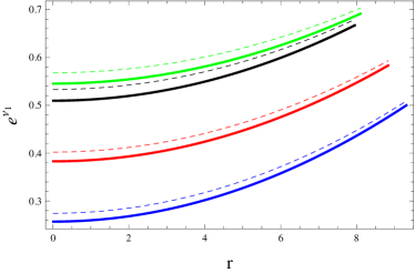
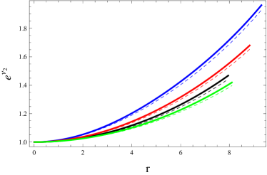
Figure 1: Metric coefficients corresponding to $\bar{\mathcal{S}}=0.2$ (thick lines), $\bar{\mathcal{S}}=0.9$ (dotted lines), $\nu_{3}=-3$ (left plot) and $\nu_{3}=3$ (right plot) for each star.

4.1 Behavior of Matter Determinants

An admissible behavior of the matter sector for isotropic/anisotropic fluid distribution requires that these parameters must be maximum and positive at $r=0$ and decreasing outward. Figure 2 exhibits an acceptable behavior of the density and radial/transverse components of pressure for chosen values of $\nu_{3}$ and charge. All these parameters gain less values in the interior of considered models for higher value of the charge. It is also noted that $\nu_{3}=3$ produces denser interiors as compared to its other adopted value. It is worthy to mention that the radial pressure in this modified gravity corresponding to each star disappears at the hypersurface. These compact systems become densest for $\nu_{3}=3$ and $\bar{\mathcal{S}}=0.2$ among all the adopted choices (Tables $\mathbf{4}-\mathbf{7}$). The regularity conditions (such as $\frac{d\mu}{dr}|_{r=0}=0,~{}\frac{dP_{r}}{dr}|_{r=0}=0,~{}\frac{d^{2}\mu}{dr^{2}}|_{r=0}<0$, $\frac{d^{2}P_{r}}{dr^{2}}|_{r=0}<0$) are also checked and observed to be satisfied.

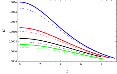
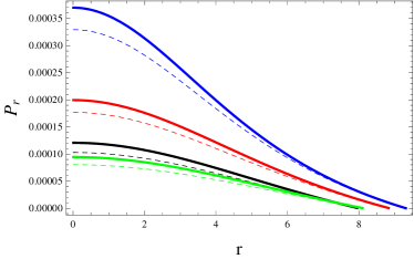
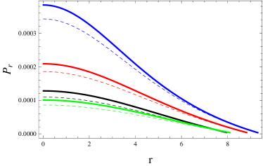
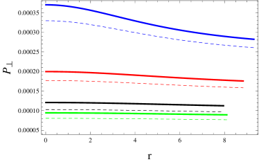
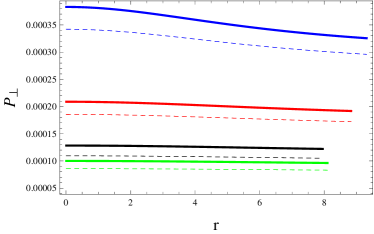
Figure 2: Matter determinants corresponding to $\bar{\mathcal{S}}=0.2$ (thick lines), $\bar{\mathcal{S}}=0.9$ (dotted lines), $\nu_{3}=-3$ (left plots) and $\nu_{3}=3$ (right plots) for each star.

4.2 Pressure Anisotropy

The anisotropy in the considered structures are defined by $\Delta=P_{\bot}-P_{r}$ which can be calculated from Eqs.(17) and (18). Since the anisotropy has a great role in the evolution of celestial systems, we check the impact of an electromagnetic field on this factor. The anisotropy disappears at the star’s center and exhibits decreasing (inward) or increasing (outward) trend on the basis whether the difference between both pressures is negative or positive, respectively. This factor is observed to be null at the core of each candidate and increase outward, as seen by Figure $\mathbf{3}$. We also notice that the increment in charge causes anisotropy to be reduced.

4.3 Mass, Compactness and Surface Redshift

A spherical structure (7) has a mass interlinked with the energy density given by

$$\bar{m}(r)=\frac{1}{2}\int_{0}^{\mathcal{H}}\breve{r}^{2}\mu d\breve{r},$$ (32)

where $\mu$ symbolizes the effective density in this modified theory and given in Eq.(21). Equations (19), (24), (29) and (30) together yields, equivalently, as

$$\bar{m}(r)=\frac{r}{2}\left[1+\frac{\bar{s}^{2}}{r^{2}}-\frac{\big{(}\mathcal{H}^{3}-\bar{\mathcal{M}}r^{2}\big{)}\big{\{}\mathcal{H}^{3}(\mathcal{H}-3\bar{\mathcal{M}})+\bar{\mathcal{M}}\mathcal{H}r^{2}-\bar{\mathcal{S}}^{2}\big{(}r^{2}-2\mathcal{H}^{2}\big{)}\big{\}}}{\mathcal{H}^{3}\big{\{}\mathcal{H}^{3}(\mathcal{H}-3\bar{\mathcal{M}})+2\bar{\mathcal{M}}\mathcal{H}r^{2}-2\bar{\mathcal{S}}^{2}\big{(}r^{2}-\mathcal{H}^{2}\big{)}\big{\}}}\right].$$ (33)

Figure 3 represents the plots of the mass function for the interior distribution of compact candidates. We observe that this function possesses an increasing behavior outward. It is also shown that the considered systems are more massive for the choices $\nu_{3}=3$ and $\bar{\mathcal{S}}=0.2$. Moreover, the increasing impact of charge provides less massive interiors.

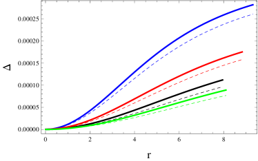
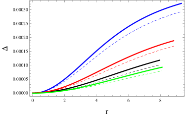
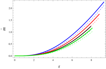
Figure 3: Anisotropy and mass corresponding to $\bar{\mathcal{S}}=0.2$ (thick lines), $\bar{\mathcal{S}}=0.9$ (dotted lines), $\nu_{3}=-3$ (left plots) and $\nu_{3}=3$ (right plots) for each star.

Some more physical parameters of compact stars must be analyzed while discussing their evolution, such as the compactness and the redshift. The former quantity (represented by $\varrho$) is defined as a ratio of mass to radius of a self-gravitating body. It is given by the following expression

$$\varrho(r) =\frac{\bar{m}(r)}{r}$$

$$=\frac{1}{2}\left[1+\frac{\bar{s}^{2}}{r^{2}}-\frac{\big{(}\mathcal{H}^{3}-\bar{\mathcal{M}}r^{2}\big{)}\big{\{}\mathcal{H}^{3}(\mathcal{H}-3\bar{\mathcal{M}})+\bar{\mathcal{M}}\mathcal{H}r^{2}-\bar{\mathcal{S}}^{2}\big{(}r^{2}-2\mathcal{H}^{2}\big{)}\big{\}}}{\mathcal{H}^{3}\big{\{}\mathcal{H}^{3}(\mathcal{H}-3\bar{\mathcal{M}})+2\bar{\mathcal{M}}\mathcal{H}r^{2}-2\bar{\mathcal{S}}^{2}\big{(}r^{2}-\mathcal{H}^{2}\big{)}\big{\}}}\right].$$ (34)

A feasible spherically symmetric solution must have the value of compactness less than $\frac{4}{9}$ everywhere in the interior configuration [68]. The later parameter, mentioned above, quantifies an increment in the electromagnetic waves (or radiations) emitted by a heavily body when it undergoes specific reactions. Mathematically, it is calculated as

$$z(r)=\frac{1-\sqrt{1-2\varrho(r)}}{\sqrt{1-2\varrho(r)}},$$ (35)

leading to

$$z(r)=-1+\bigg{[}\frac{\big{(}\mathcal{H}^{3}-\bar{\mathcal{M}}r^{2}\big{)}\big{\{}\mathcal{H}^{3}(\mathcal{H}-3\bar{\mathcal{M}})+\bar{\mathcal{M}}\mathcal{H}r^{2}-\bar{\mathcal{S}}^{2}\big{(}r^{2}-2\mathcal{H}^{2}\big{)}\big{\}}}{\mathcal{H}^{3}\big{\{}\mathcal{H}^{3}(\mathcal{H}-3\bar{\mathcal{M}})+2\bar{\mathcal{M}}\mathcal{H}r^{2}-2\bar{\mathcal{S}}^{2}\big{(}r^{2}-\mathcal{H}^{2}\big{)}\big{\}}}-\frac{\bar{s}^{2}}{r^{2}}\bigg{]}^{-\frac{1}{2}}.$$ (36)

Buchdahl determined its maximum value at the hypersurface for isotropic matter as $2$ which was later found to be $5.211$ for anisotropic interior [74]. We plot both of these parameters in Figure $\mathbf{4}$ for all choices of parameters and obtain compatible behavior with the observational data. The increment in charge and decrement in the bag constant decrease these entities. Their values at $\Sigma:r=\mathcal{H}$ are provided in Tables $\mathbf{4}-\mathbf{7}$ for all parametric values.

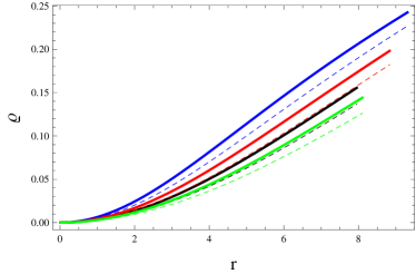
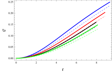
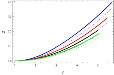
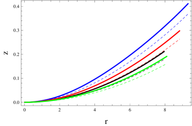
Figure 4: Compactness and redshift corresponding to $\bar{\mathcal{S}}=0.2$ (thick lines), $\bar{\mathcal{S}}=0.9$ (dotted lines), $\nu_{3}=-3$ (left plots) and $\nu_{3}=3$ (right plots) for each star.

4.4 Energy Conditions

In this subsection, we present some constraints through which the existence of usual or exotic fluid in an interior geometry can be confirmed. These bounds depend explicitly on state determinants and are used extensively in the literature, titled as energy conditions. Their satisfaction results in the presence of normal fluid in a compact interior, thus leads to a viable model. Otherwise, there must be an exotic matter inside a spherical geometry. They are given as follows

• Dominant: $\mu-P_{\bot}\geq 0$,  $\mu-P_{r}+\frac{\bar{s}^{2}}{4\pi r^{4}}\geq 0$,

• Strong: $\mu+2P_{\bot}+P_{r}+\frac{\bar{s}^{2}}{4\pi r^{4}}\geq 0$,

• Weak: $\mu+\frac{\bar{s}^{2}}{8\pi r^{4}}\geq 0$,  $\mu+P_{\bot}+\frac{\bar{s}^{2}}{4\pi r^{4}}\geq 0$,  $\mu+P_{r}\geq 0$,

• Null: $\mu+P_{\bot}+\frac{\bar{s}^{2}}{4\pi r^{4}}\geq 0$,  $\mu+P_{r}\geq 0$.

Figures 5 and 6 exhibit such bounds for $\nu_{3}=-3$ and $3$, respectively. We notice that all these conditions satisfy everywhere for both values of charge, representing a viable extended solution in $\mathcal{R}+\nu_{3}\mathcal{Q}$ gravity. It is worthy to mention that we observe a contradiction of these results with those of provided in [16].

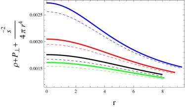
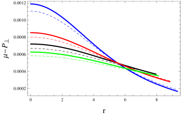
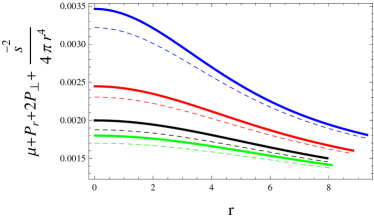
Figure 5: Energy conditions corresponding to $\nu_{3}=-3$ with $\bar{\mathcal{S}}=0.2$ (thick lines) and $\bar{\mathcal{S}}=0.9$ (dotted lines) for each star.

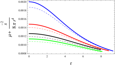
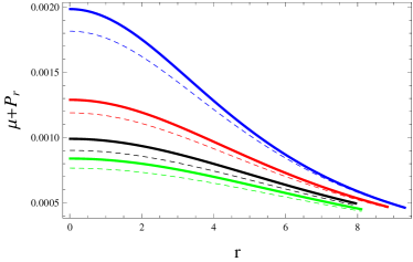
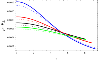
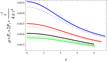
Figure 6: Energy conditions corresponding to $\nu_{3}=3$ with $\bar{\mathcal{S}}=0.2$ (thick lines) and $\bar{\mathcal{S}}=0.9$ (dotted lines) for each star.

4.5 Tolman-Opphenheimer-Volkoff Equation

In this subsection, we plot different forces involving in the Tolman-Opphenheimer-Volkoff ($\mathbb{TOV}$) equation corresponding to this modified theory to check whether the developed model is in stable equilibrium or not [75, 76]. We obtain the following $\mathbb{TOV}$ equation from Eq.(15) given by

$$\frac{dP_{r}}{dr}+\frac{\nu_{1}^{\prime}}{2}\left(\mu+P_{r}\right)-\frac{2}{r}\left(P_{\bot}-P_{r}\right)-\frac{2\nu_{3}}{e^{\nu_{2}}\big{(}\nu_{3}\mathcal{R}+16\pi\big{)}}\bigg{[}\frac{\nu_{1}^{\prime}\mu}{8}\bigg{(}\nu_{1}^{\prime 2}+2\nu_{1}^{\prime\prime}$$

$$-\nu_{1}^{\prime}\nu_{2}^{\prime}+\frac{4\nu_{1}^{\prime}}{r}\bigg{)}-\frac{\mu^{\prime}}{8}\bigg{(}\nu_{1}^{\prime 2}-\nu_{1}^{\prime}\nu_{2}^{\prime}+2\nu_{1}^{\prime\prime}+\frac{4\nu_{1}^{\prime}}{r}\bigg{)}+P_{r}\bigg{(}\frac{5\nu_{1}^{\prime 2}\nu_{2}^{\prime}}{8}-\frac{5\nu_{1}^{\prime}\nu_{2}^{\prime 2}}{8}$$

$$-\frac{5\nu_{2}^{\prime 2}}{2r}+\frac{7\nu_{1}^{\prime\prime}\nu_{2}^{\prime}}{4}-\frac{\nu_{1}^{\prime\prime\prime}}{2}-\nu_{1}^{\prime}\nu_{1}^{\prime\prime}+\frac{\nu_{1}^{\prime}\nu_{2}^{\prime\prime}}{2}+\frac{2\nu_{2}^{\prime\prime}}{r}+\frac{\nu_{1}^{\prime}\nu_{2}^{\prime}}{r}-\frac{\nu_{2}^{\prime}}{r^{2}}-\frac{\nu_{1}^{\prime\prime}}{r}+\frac{\nu_{1}^{\prime}}{r^{2}}$$

$$+\frac{2e^{\nu_{2}}}{r^{3}}-\frac{2}{r^{3}}\bigg{)}+\frac{P^{\prime}_{r}}{8}\bigg{(}\nu_{1}^{\prime}\nu_{2}^{\prime}-2\nu_{1}^{\prime\prime}-\nu_{1}^{\prime 2}+\frac{4\nu_{2}^{\prime}}{r}\bigg{)}+\frac{P_{\bot}}{r^{2}}\bigg{(}\nu_{2}^{\prime}-\nu_{1}^{\prime}+\frac{2e^{\nu_{2}}}{r}$$

$$-\frac{2}{r}\bigg{)}-\frac{P^{\prime}_{\bot}}{r}\bigg{(}\frac{\nu_{2}^{\prime}}{2}-\frac{\nu_{1}^{\prime}}{2}+\frac{e^{\nu_{2}}}{r}-\frac{1}{r}\bigg{)}-\left(\frac{\nu_{1}^{\prime}}{r}-\frac{e^{\nu_{2}}}{r^{2}}+\frac{1}{r^{2}}+\frac{2e^{\nu_{2}}}{\nu_{3}}\right)$$

$$\times\bigg{(}\frac{\bar{s}\bar{s}^{\prime}}{r^{4}}-\frac{2\bar{s}^{2}}{r^{5}}\bigg{)}\bigg{]}=0.$$ (37)

The compact notation of the above equation is

$$f_{h}+f_{a}+f_{g}=0,$$ (38)

where $f_{h},~{}f_{a}$ and $f_{g}$ are hydrostatic, anisotropic and gravitational, respectively, provided as

$$f_{h} =-\frac{dP_{r}}{dr},$$

$$f_{a} =\frac{2}{r}\big{(}P_{\bot}-P_{r}\big{)},$$

and $f_{g}$ contains all remaining terms of Eq.(37) with opposite sign. Figure 7 indicates that the interiors of all considered quark are in the hydrostatic equilibrium.

4.6 Stability Analysis

Stability plays a major role in studying the evolutionary patterns of an astrophysical structure in our cosmos. The following lines shall help us to study the stability of the considered modified model (11) with the help of three approaches.

4.6.1 Causality Condition and Herrera Cracking Technique

Since the fluid under consideration is anisotropic in nature, there exist two sound speeds in tangential and radial directions that must be less than the speed of light according to the causality condition [77], i.e.,

$$0<v_{s\bot}^{2}=\frac{dP_{\bot}}{d\mu}<1,\quad 0<v_{sr}^{2}=\frac{dP_{r}}{d\mu}<1.$$ (39)

We obtain $v_{sr}^{2}=\frac{1}{3}\in(0,1)$, thus do not need to plot it. Furthermore, Figure 8 (upper plots) shows the tangential sound speed. All candidates are appeared to be stable for chosen parametric values except SAX J 1808.4-3658 which is unstable only for $\nu_{3}=3$ and $\bar{\mathcal{S}}=0.9$.

The above two sound speeds are combined by Herrera [78] in a single frame, known as cracking condition. According to this, a stable interior can be obtained only if the following condition holds

$$0<\mid v_{s\bot}^{2}-v_{sr}^{2}\mid<1.$$ (40)

The lower plots of Figure 8 manifest that the considered stars are stable for $\nu_{3}=-3$. However, two compact structures such as SMC X-4 and SAX J 1808.4-3658 are unstable for $\bar{\mathcal{S}}=0.9$ and both choices of charge along with $\nu_{3}=3$, respectively.

4.6.2 Adiabatic Index

Another effective tool, in this regard, is the adiabatic index that helps to check whether a system is stable or unstable. This technique has been extensively discussed and used in the literature [79], and it was found that the value of this index ($\Gamma_{\mathrm{ad}}$) greater than $\frac{4}{3}$ leads to stable models. Here, we define it as

$$\Gamma_{\mathrm{ad}}=\frac{P_{r}+\mu}{P_{r}}\left(\frac{dP_{r}}{d\mu}\right)=\frac{P_{r}+\mu}{P_{r}}\left(v_{sr}^{2}\right).$$ (41)

Figure 9 depicts the graph of $\Gamma_{\mathrm{ad}}$ from which stable compact models are achieved everywhere for all parametric values.

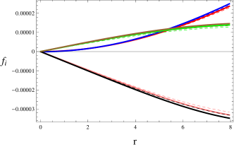
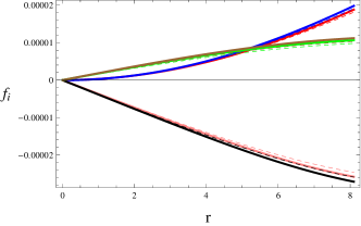
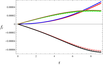
Figure 7: Variation in $f_{g}$ (black, pink), $f_{a}$ (red, blue) and $f_{h}$ (brown, green) corresponding to SMC X-4 (upper left), SAX J 1808.4-3658 (upper right), Her X-I (lower left) and 4U 1820-30 (lower right).

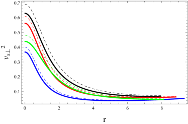
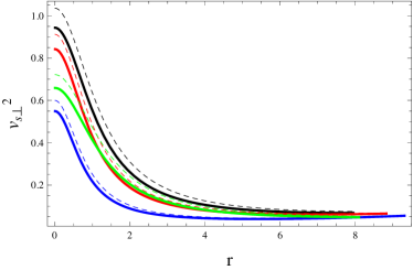
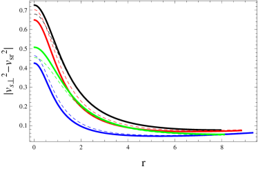
Figure 8: Tangential sound speed and $\mid v_{s\bot}^{2}-v_{sr}^{2}\mid$ corresponding to $\bar{\mathcal{S}}=0.2$ (thick lines), $\bar{\mathcal{S}}=0.9$ (dotted lines), $\nu_{3}=-3$ (left plots) and $\nu_{3}=3$ (right plots) for each star.

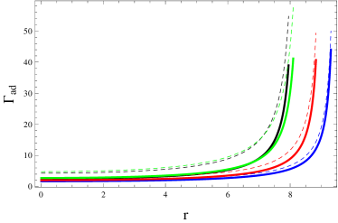
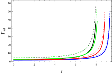
Figure 9: Adiabatic index corresponding to $\bar{\mathcal{S}}=0.2$ (thick lines), $\bar{\mathcal{S}}=0.9$ (dotted lines), $\nu_{3}=-3$ (left plot) and $\nu_{3}=3$ (right plot) for each star.

5 Conclusions

This paper discusses the impact of an electromagnetic field and the non-minimal matter-geometry coupling on different quark star candidates through a linear model $\mathcal{R}+\nu_{3}\mathcal{Q}$ by choosing the coupling constant as $\nu_{3}=\pm 3$. However, the question arises in ones mind that why we have taken such large values of the model parameter. Since we aimed to show that how physical properties in the compact interiors behave by varying the coupling parameter in this modified theory, those parametric values must be taken which show the desired difference. In this regard, we have initially done the whole analysis for small positive/negative values of $\nu_{3}$, and found same profile of physical characteristics everywhere for both considered values. However, we have not included their plots in the paper. The matter Lagrangian density for the charged fluid was taken as $\mathbf{L}_{m}=-\frac{1}{4}\mathcal{Z}_{\beta\xi}\mathcal{Z}^{\beta\xi}$ [14], leading to $\mathbf{L}_{m}=\frac{\bar{s}^{2}}{2r^{4}}$. The field equations and hydrostatic equilibrium condition have been formulated in this modified theory. We have chosen $g_{tt}$ and $g_{rr}$ metric functions of Tolman IV spacetime, and a particular expression for the charge to reduce the number of unknowns in the system of equations (21)-(23). We have chosen four star candidates such as SMC X-4, SAX J 1808.4-3658, Her X-I and 4U 1820-30 whose masses and radii are presented in Table 1. The unknown triplet ($\mathcal{A}_{1},\mathcal{A}_{2},\mathcal{A}_{3}$) in Tolman IV spacetime has also been calculated at the spherical boundary in terms of experimentally observed data (radii and masses) of quark models. This triplet has been calculated in Tables 2 and 3 for two different values of the charge as 0.2 and 0.9, respectively. We have plotted several physical properties of self-gravitating systems for different choices of coupling constant and charge. The developed state determinants are maximum/minimum at the center/boundary for each star candidate, leading to a physically acceptable model. The mass and anisotropy have shown increasing behavior towards the spherical boundary for all choices of parameters (Figure $\mathbf{3}$).

We have also noticed that the densest interiors of different considered stars in this theory correspond to the positive choice of $\nu_{3}$ along with less charge among all four discussed choices. The trend of redshift and compactness has been detected as compatible. The energy bounds are satisfied everywhere in the interior region of each star, resulting in the viability of our developed model. We have noticed that the increment in charge makes the considered compact interiors less dense for both values of the model parameter (Figure 2). Moreover, the presence of charge produced less anisotropic structures (Figure 3). It must be mentioned here that the interaction between gravity and an electromagnetic field has been used to study the role of corresponding equations of motion on the fields of purely physical nature [80]. The central density, surface density as well as central radial pressure have been evaluated in the interior of a compact candidate Her X-1 in the context of $\mathbb{GR}$ [81], from which we found that this modified theory gains higher values in comparison with the existing outcomes. We have also noticed the interior of Her X-1 in this gravity to be the less dense as compared to that in $f(\mathcal{G})$ theory [82]. Further, the interior of the quark star SAX J 1808.4-3658 has been explored in $f(\mathcal{R},\mathcal{T})$ theory [83] and found to be less dense as opposed to $f(\mathcal{R},\mathcal{T},\mathcal{Q})$ framework. It is also observed that more suitable results are obtained in $f(\mathcal{R},\mathcal{T},\mathcal{R}_{\beta\xi}\mathcal{T}^{\beta\xi})$ theory for $\nu_{3}=-3$ as compared to [19, 20] and the solution corresponding to $\nu_{3}=3$. Finally, stability has been observed through different approaches. It is concluded that only two quark stars such as Her X-I and 4U 1820-30 exhibit stable behavior for all parametric choices, thus these results are consistent with [84]. However, the remaining models, namely SMC X-4 and SAX J 1808.4-3658 have shown stable behavior only for the negative value of the coupling constant (Figure $\mathbf{8}$). On the other hand, the compact star SMC X-4 was found to be stable for lower charge with $\nu_{3}=3$, however, the increment in charge made it unstable. It must be mentioned here that our results in this modified theory reduce to $\mathbb{GR}$ for $\nu_{3}=0$.

Appendix A

The matter sector (21)-(23) in terms of Tolman IV spacetime is given by

$$\mu =\frac{1}{r^{4}}\big{[}d_{1}^{4}\big{\{}32\pi d_{3}^{2}-d_{3}\big{(}19\nu_{3}+32\pi r^{2}\big{)}+16\nu_{3}r^{2}\big{\}}+2d_{1}^{3}\big{\{}2d_{3}^{2}\big{(}\nu_{3}+56\pi r^{2}\big{)}$$

$$-d_{3}\big{(}112\pi r^{4}+69\nu_{3}r^{2}\big{)}+58\nu_{3}r^{4}\big{\}}+d_{1}\big{\{}10d_{3}^{2}\big{(}64\pi r^{6}+5\nu_{3}r^{4}\big{)}-4d_{3}$$

$$\times\big{(}160\pi r^{8}+111\nu_{3}r^{6}\big{)}+358\nu_{3}r^{8}\big{\}}-4r^{6}\big{\{}d_{3}\big{(}64\pi r^{4}+41\nu_{3}r^{2}\big{)}-34\nu_{3}r^{4}$$

$$-4d_{3}^{2}\big{(}\nu_{3}+16\pi r^{2}\big{)}\big{\}}+d_{1}^{2}\big{\{}6d_{3}^{2}\big{(}96\pi r^{4}+5\nu_{3}r^{2}\big{)}-d_{3}\big{(}576\pi r^{6}+383\nu_{3}r^{4}\big{)}$$

$$+314\nu_{3}r^{6}\big{\}}\big{]}^{-1}\big{[}d_{1}^{4}\big{\{}32\pi\mathrm{B}d_{3}^{2}r^{4}+d_{3}\big{(}-32\pi\mathrm{B}r^{6}+r^{4}(6-40\nu_{3}\mathrm{B})+3\nu_{3}\bar{s}^{2}\big{)}$$

$$+r^{6}(28\nu_{3}\mathrm{B}-6)-3\nu_{3}r^{2}\bar{s}^{2}\big{\}}-4r^{6}\big{\{}d_{3}\big{(}64\pi\mathrm{B}r^{8}+r^{6}(68\nu_{3}\mathrm{B}+6)+3\nu_{3}r^{2}\bar{s}^{2}\big{)}$$

$$-d_{3}^{2}\big{(}64\pi\mathrm{B}r^{6}+r^{4}(4\nu_{3}\mathrm{B}+6)+3\nu_{3}\bar{s}^{2}\big{)}-52\nu_{3}\mathrm{B}r^{8}\big{\}}+2d_{1}r^{4}\big{\{}d_{3}^{2}\big{(}320\pi\mathrm{B}r^{6}$$

$$+r^{4}(4\nu_{3}\mathrm{B}+30)+15\nu_{3}\bar{s}^{2}\big{)}-4d_{3}\big{(}80\pi\mathrm{B}r^{8}+r^{6}(84\nu_{3}\mathrm{B}+6)+3\nu_{3}r^{2}\bar{s}^{2}\big{)}$$

$$+r^{8}(260\nu_{3}\mathrm{B}-6)-3\nu_{3}r^{4}\bar{s}^{2}\big{\}}+d_{1}^{2}r^{2}\big{\{}12d_{3}^{2}\big{(}48\pi\mathrm{B}r^{6}+r^{4}(4-3\nu_{3}\mathrm{B})$$

$$+2\nu_{3}\bar{s}^{2}\big{)}-d_{3}\big{(}576\pi\mathrm{B}r^{8}+2r^{6}(286\nu_{3}\mathrm{B}+9)+9\nu_{3}r^{2}\bar{s}^{2}\big{)}+r^{8}(452\nu_{3}\mathrm{B}-30)$$

$$-15\nu_{3}r^{4}\bar{s}^{2}\big{\}}+2d_{1}^{3}\big{\{}d_{3}^{2}\big{(}112\pi\mathrm{B}r^{6}+r^{4}(6-10\nu_{3}\mathrm{B})+3\nu_{3}\bar{s}^{2}\big{)}+d_{3}\big{(}3\nu_{3}r^{2}\bar{s}^{2}$$

$$-112\pi\mathrm{B}r^{8}+r^{6}(6-114\nu_{3}\mathrm{B})\big{)}+4r^{8}(22\nu_{3}\mathrm{B}-3)-6\nu_{3}r^{4}\bar{s}^{2}\big{\}}\big{]},$$ (A1)

$$P_{r} =\frac{1}{r^{4}}\big{[}d_{1}^{4}\big{\{}32\pi d_{3}^{2}-d_{3}\big{(}19\nu_{3}+32\pi r^{2}\big{)}+16\nu_{3}r^{2}\big{\}}+2d_{1}^{3}\big{\{}2d_{3}^{2}\big{(}\nu_{3}+56\pi r^{2}\big{)}$$

$$-d_{3}\big{(}112\pi r^{4}+69\nu_{3}r^{2}\big{)}+58\nu_{3}r^{4}\big{\}}+d_{1}\big{\{}10d_{3}^{2}\big{(}64\pi r^{6}+5\nu_{3}r^{4}\big{)}-4d_{3}$$

$$\times\big{(}160\pi r^{8}+111\nu_{3}r^{6}\big{)}+358\nu_{3}r^{8}\big{\}}-4r^{6}\big{\{}d_{3}\big{(}64\pi r^{4}+41\nu_{3}r^{2}\big{)}-34\nu_{3}r^{4}$$

$$-4d_{3}^{2}\big{(}\nu_{3}+16\pi r^{2}\big{)}\big{\}}+d_{1}^{2}\big{\{}6d_{3}^{2}\big{(}96\pi r^{4}+5\nu_{3}r^{2}\big{)}-d_{3}\big{(}576\pi r^{6}+383\nu_{3}r^{4}\big{)}$$

$$+314\nu_{3}r^{6}\big{\}}\big{]}^{-1}\big{[}\big{(}d_{1}+2r^{2}\big{)}\big{(}r^{2}-d_{3}\big{)}\big{\{}d_{1}^{3}\big{(}32\pi\mathrm{B}d_{3}r^{4}-2r^{4}(6\nu_{3}\mathrm{B}+1)$$

$$-\nu_{3}\bar{s}^{2}\big{)}-2r^{4}\big{(}d_{3}\big{(}-64\pi\mathrm{B}r^{6}+r^{4}(2-4\nu_{3}\mathrm{B})+\nu_{3}\bar{s}^{2}\big{)}+28\nu_{3}\mathrm{B}r^{6}\big{)}-2d_{1}^{2}$$

$$\times\big{(}d_{3}\big{(}-80\pi\mathrm{B}r^{6}+r^{4}(2-6\nu_{3}\mathrm{B})+\nu_{3}\bar{s}^{2}\big{)}+r^{6}(36\nu_{3}\mathrm{B}+2)+\nu_{3}r^{2}\bar{s}^{2}\big{)}$$

$$+d_{1}\big{(}4d_{3}\big{(}64\pi\mathrm{B}r^{8}+r^{6}(7\nu_{3}\mathrm{B}-2)-\nu_{3}r^{2}\bar{s}^{2}\big{)}-2r^{8}(62\nu_{3}\mathrm{B}+1)-\nu_{3}r^{4}\bar{s}^{2}\big{)}\big{\}}\big{]},$$ (A2)

$$P_{\bot} =\big{[}2d_{3}r^{4}\big{(}d_{1}+2r^{2}\big{)}\big{\{}d_{1}^{2}\big{(}8\pi d_{3}-3\nu_{3}\big{)}+d_{1}r^{2}\big{(}32\pi d_{3}-11\nu_{3}\big{)}+2\big{(}d_{3}r^{2}$$

$$\times\big{(}\nu_{3}+16\pi r^{2}\big{)}-6\nu_{3}r^{4}\big{)}\big{\}}\big{\{}d_{1}^{4}\big{(}d_{3}\big{(}19\nu_{3}+32\pi r^{2}\big{)}-32\pi d_{3}^{2}-16\nu_{3}r^{2}\big{)}-2d_{1}^{3}$$

$$\times\big{(}2d_{3}^{2}\big{(}\nu_{3}+56\pi r^{2}\big{)}-d_{3}\big{(}112\pi r^{4}+69\nu_{3}r^{2}\big{)}+58\nu_{3}r^{4}\big{)}+d_{1}\big{(}d_{3}\big{(}640\pi r^{8}$$

$$+444\nu_{3}r^{6}\big{)}-10d_{3}^{2}\big{(}64\pi r^{6}+5\nu_{3}r^{4}\big{)}-358\nu_{3}r^{8}\big{)}+4r^{6}\big{(}d_{3}\big{(}64\pi r^{4}+41\nu_{3}r^{2}\big{)}$$

$$-4d_{3}^{2}\big{(}\nu_{3}+16\pi r^{2}\big{)}-34\nu_{3}r^{4}\big{)}+d_{1}^{2}\big{(}d_{3}\big{(}576\pi r^{6}+383\nu_{3}r^{4}\big{)}-314\nu_{3}r^{6}$$

$$-6d_{3}^{2}\big{(}96\pi r^{4}+5\nu_{3}r^{2}\big{)}\big{)}\big{\}}\big{]}^{-1}\big{[}8\big{\{}612\bar{s}^{2}\nu_{3}^{3}r^{8}-4\nu_{3}\big{(}2(62\nu_{3}\mathrm{B}-51)r^{6}+12$$

$$\times(17+58\pi)\bar{s}^{2}\nu_{3}r^{2}+261\bar{s}^{2}\nu_{3}^{2}\big{)}d_{3}r^{6}+\big{(}3072\pi^{2}\bar{s}^{2}\nu_{3}r^{4}+16\pi\big{(}232\bar{s}^{2}\nu_{3}r^{4}$$

$$+16(4\nu_{3}\mathrm{B}-3)r^{8}+265\bar{s}^{2}\nu_{3}^{2}r^{2}\big{)}+\nu_{3}\big{(}(472\nu_{3}\mathrm{B}-644)r^{6}+1112\bar{s}^{2}\nu_{3}r^{2}$$

$$+475\bar{s}^{2}\nu_{3}^{2}\big{)}\big{)}d_{3}^{2}r^{4}-\big{(}4096\pi^{2}\bar{s}^{2}\big{(}r^{2}+\nu_{3}\big{)}r^{4}+16\pi\big{(}276\bar{s}^{2}\nu_{3}r^{4}+93\bar{s}^{2}\nu_{3}^{2}r^{2}\big{)}$$

$$+16(3\nu_{3}\mathrm{B}-4)r^{8}+\nu_{3}\big{(}4(12\nu_{3}\mathrm{B}-55)r^{6}+256\bar{s}^{2}\nu_{3}r^{2}+77\bar{s}^{2}\nu_{3}^{2}\big{)}\big{)}d_{3}^{3}r^{2}$$

$$+4\big{(}256\pi^{2}\bar{s}^{2}\big{(}4r^{2}+\nu_{3}\big{)}r^{4}+\nu_{3}\big{(}-4r^{6}+4\bar{s}^{2}\nu_{3}r^{2}+\bar{s}^{2}\nu_{3}^{2}\big{)}-32\pi\big{(}2r^{8}$$

$$-4\bar{s}^{2}\nu_{3}r^{4}-\bar{s}^{2}\nu_{3}^{2}r^{2}\big{)}\big{)}d_{3}^{4}\big{\}}r^{8}-4d_{1}\big{\{}-4752\bar{s}^{2}\nu_{3}^{3}r^{8}+2\nu_{3}\big{(}10(222\nu_{3}\mathrm{B}-161)$$

$$\times r^{6}+4(827+2698\pi)\bar{s}^{2}\nu_{3}r^{2}+3947\bar{s}^{2}\nu_{3}^{2}\big{)}d_{3}r^{6}-4\big{(}5888\pi^{2}\bar{s}^{2}\nu_{3}r^{4}+4\pi$$

$$\times\big{(}16(33\nu_{3}\mathrm{B}-23)r^{8}+1876\bar{s}^{2}\nu_{3}r^{4}+2013\bar{s}^{2}\nu_{3}^{2}r^{2}\big{)}+\nu_{3}\big{(}(430\nu_{3}\mathrm{B}-419)$$

$$\times 3r^{6}+2234\bar{s}^{2}\nu_{3}r^{2}+835\bar{s}^{2}\nu_{3}^{2}\big{)}\big{)}d_{3}^{2}r^{4}+\big{(}2048\pi^{2}\bar{s}^{2}\big{(}16r^{2}+15\nu_{3}\big{)}r^{4}+16\pi$$

$$\times\big{(}16(29\nu_{3}\mathrm{B}-30)r^{8}+2228\bar{s}^{2}\nu_{3}r^{4}+663\bar{s}^{2}\nu_{3}^{2}r^{2}\big{)}+\nu_{3}\big{(}4(368\nu_{3}\mathrm{B}-401)r^{6}$$

$$+1944\bar{s}^{2}\nu_{3}r^{2}+499\bar{s}^{2}\nu_{3}^{2}\big{)}\big{)}d_{3}^{3}r^{2}-\big{(}1024\pi^{2}\bar{s}^{2}\big{(}32r^{2}+7\nu_{3}\big{)}r^{4}+16\pi\big{(}16r^{8}$$

$$\times(5\nu_{3}\mathrm{B}-7)+244\bar{s}^{2}\nu_{3}r^{4}+53\bar{s}^{2}\nu_{3}^{2}r^{2}\big{)}+\nu_{3}\big{(}(80\nu_{3}\mathrm{B}-92)r^{6}+136\bar{s}^{2}\nu_{3}r^{2}$$

$$+25\bar{s}^{2}\nu_{3}^{2}\big{)}\big{)}d_{3}^{4}\big{\}}r^{6}-2d_{1}^{2}\big{\{}-15067\bar{s}^{2}\nu_{3}^{3}r^{8}+\nu_{3}\big{(}8(1911\nu_{3}\mathrm{B}-1297)r^{6}+24$$

$$\times(919+2880\pi)\bar{s}^{2}\nu_{3}r^{2}+23881\bar{s}^{2}\nu_{3}^{2}\big{)}d_{3}r^{6}-2\big{(}37888\pi^{2}\bar{s}^{2}\nu_{3}r^{4}+16\pi\big{(}296$$

$$\times(3\nu_{3}\mathrm{B}-2)r^{8}+3154\bar{s}^{2}\nu_{3}r^{4}+3117\bar{s}^{2}\nu_{3}^{2}r^{2}\big{)}+\nu_{3}\big{(}(9424\nu_{3}\mathrm{B}-7924)r^{6}$$

$$+14480\bar{s}^{2}\nu_{3}r^{2}+4359\bar{s}^{2}\nu_{3}^{2}\big{)}\big{)}d_{3}^{2}r^{4}+2\big{(}1024\pi^{2}\bar{s}^{2}\big{(}54r^{2}+47\nu_{3}\big{)}r^{4}+16\pi\big{(}16$$

$$\times(51\nu_{3}\mathrm{B}-47)r^{8}+3704\bar{s}^{2}\nu_{3}r^{4}+915\bar{s}^{2}\nu_{3}^{2}r^{2}\big{)}+\nu_{3}\big{(}20(164\nu_{3}\mathrm{B}-111)r^{6}$$

$$+2632\bar{s}^{2}\nu_{3}r^{2}+501\bar{s}^{2}\nu_{3}^{2}\big{)}\big{)}d_{3}^{3}r^{2}-2\big{(}2048\pi^{2}\bar{s}^{2}\big{(}27r^{2}+5\nu_{3}\big{)}r^{4}+\nu_{3}\big{(}60$$

$$\times(3\nu_{3}\mathrm{B}-1)r^{6}+164\bar{s}^{2}\nu_{3}r^{2}+15\bar{s}^{2}\nu_{3}^{2}\big{)}+32\pi\big{(}20(5\nu_{3}\mathrm{B}-4)r^{8}+173\bar{s}^{2}\nu_{3}r^{4}$$

$$+30\bar{s}^{2}\nu_{3}^{2}r^{2}\big{)}\big{)}d_{3}^{4}\big{\}}r^{4}+d_{1}^{4}\big{\{}13150\bar{s}^{2}\nu_{3}^{3}r^{6}-8\nu_{3}\big{(}3(598\nu_{3}\mathrm{B}-379)r^{6}+4(673$$

$$+1922\pi)\bar{s}^{2}\nu_{3}r^{2}+2328\bar{s}^{2}\nu_{3}^{2}\big{)}d_{3}r^{4}+\big{(}69120\pi^{2}\bar{s}^{2}\nu_{3}r^{4}+8\pi\big{(}(73\nu_{3}\mathrm{B}-45)$$

$$\times 48r^{8}+12548\bar{s}^{2}\nu_{3}r^{4}+10139\bar{s}^{2}\nu_{3}^{2}r^{2}\big{)}+\nu_{3}\big{(}4247\bar{s}^{2}\nu_{3}^{2}+26288\bar{s}^{2}\nu_{3}r^{2}$$

$$+2(7724\nu_{3}\mathrm{B}-6689)r^{6}\big{)}\big{)}d_{3}^{2}r^{2}+4\big{(}640\pi^{2}r^{2}\big{(}44r^{2}+5\nu_{3}\big{)}\bar{s}^{2}+\nu_{3}\big{(}34\bar{s}^{2}\nu_{3}$$

$$+(37-70\nu_{3}\mathrm{B})r^{4}\big{)}+4\pi\big{(}40(7\nu_{3}\mathrm{B}-5)r^{6}+350\bar{s}^{2}\nu_{3}r^{2}+27\bar{s}^{2}\nu_{3}^{2}\big{)}\big{)}d_{3}^{4}-2$$

$$\times\big{(}5120\pi^{2}\bar{s}^{2}\big{(}11r^{2}+8\nu_{3}\big{)}r^{4}+4\pi\big{(}16(169\nu_{3}\mathrm{B}-160)r^{8}+14268\bar{s}^{2}\nu_{3}r^{4}$$

$$+1995\bar{s}^{2}\nu_{3}^{2}r^{2}\big{)}+\nu_{3}\big{(}3(734\nu_{3}\mathrm{B}-433)r^{6}+1166\bar{s}^{2}\nu_{3}r^{2}+90\bar{s}^{2}\nu_{3}^{2}\big{)}\big{)}d_{3}^{3}\big{\}}r^{2}$$

$$+d_{1}^{3}\big{\{}25874\bar{s}^{2}\nu_{3}^{3}r^{8}-\nu_{3}\big{(}620(44\nu_{3}\mathrm{B}-29)r^{6}+8(4997+15002\pi)\bar{s}^{2}\nu_{3}r^{2}$$

$$+38819\bar{s}^{2}\nu_{3}^{2}\big{)}d_{3}r^{6}+\big{(}133120\pi^{2}\bar{s}^{2}\nu_{3}r^{4}+16\pi\big{(}11556\bar{s}^{2}\nu_{3}r^{4}+10379\bar{s}^{2}\nu_{3}^{2}r^{2}$$

$$+16(201\nu_{3}\mathrm{B}-130)r^{8}\big{)}+\nu_{3}\big{(}4(8104\nu_{3}\mathrm{B}-6709)r^{6}+50648\bar{s}^{2}\nu_{3}r^{2}$$

$$+11569\bar{s}^{2}\nu_{3}^{2}\big{)}\big{)}d_{3}^{2}r^{4}-4\big{(}10240\pi^{2}\bar{s}^{2}\big{(}5r^{2}+4\nu_{3}\big{)}r^{4}+4\pi\big{(}(11\nu_{3}\mathrm{B}-10)$$

$$\times 256r^{8}+13360\bar{s}^{2}\nu_{3}r^{4}+2579\bar{s}^{2}\nu_{3}^{2}r^{2}\big{)}+\nu_{3}\big{(}1732\bar{s}^{2}\nu_{3}r^{2}+222\bar{s}^{2}\nu_{3}^{2}+r^{6}$$

$$\times(2726\nu_{3}\mathrm{B}-1579)\big{)}\big{)}d_{3}^{3}r^{2}+4\big{(}2560\pi^{2}\bar{s}^{2}\big{(}20r^{2}+3\nu_{3}\big{)}r^{4}+4\pi\big{(}(3\nu_{3}\mathrm{B}-2)$$

$$\times 240r^{8}+964\bar{s}^{2}\nu_{3}r^{4}+121\bar{s}^{2}\nu_{3}^{2}r^{2}\big{)}+\nu_{3}\big{(}(26\nu_{3}\mathrm{B}+23)r^{6}+96\bar{s}^{2}\nu_{3}r^{2}$$

$$+2\bar{s}^{2}\nu_{3}^{2}\big{)}\big{)}d_{3}^{4}\big{\}}r^{2}+d_{1}^{7}\big{\{}512\pi^{2}\bar{s}^{2}d_{3}^{4}-16\pi\big{(}(8\nu_{3}\mathrm{B}-4)r^{4}+32\pi\bar{s}^{2}r^{2}+\bar{s}^{2}\nu_{3}$$

$$\times(31+16\pi)\big{)}d_{3}^{3}+2\big{(}128\pi^{2}r^{2}\nu_{3}\bar{s}^{2}+4\pi\big{(}56\bar{s}^{2}\nu_{3}r^{2}+31\bar{s}^{2}\nu_{3}^{2}+(3\nu_{3}\mathrm{B}-1)$$

$$\times 8r^{6}\big{)}+\nu_{3}\big{(}3(8\nu_{3}\mathrm{B}-5)r^{4}+59\bar{s}^{2}\nu_{3}\big{)}\big{)}d_{3}^{2}-\nu_{3}\big{(}4(18\nu_{3}\mathrm{B}-5)r^{6}+2\bar{s}^{2}\nu_{3}r^{2}$$

$$\times(51+112\pi)+57\bar{s}^{2}\nu_{3}^{2}\big{)}d_{3}+48r^{2}\bar{s}^{2}\nu_{3}^{3}\big{\}}+d_{1}^{6}\big{\{}668\bar{s}^{2}\nu_{3}^{3}r^{4}-2\nu_{3}\big{(}40r^{6}$$

$$\times(11\nu_{3}\mathrm{B}-5)+2(317+784\pi)\bar{s}^{2}\nu_{3}r^{2}+421\bar{s}^{2}\nu_{3}^{2}\big{)}d_{3}r^{2}+64\pi\big{(}104\pi\bar{s}^{2}r^{2}$$

$$-r^{4}+(1+4\pi)\bar{s}^{2}\nu_{3}\big{)}d_{3}^{4}-2\big{(}128\pi^{2}r^{2}\big{(}26r^{2}+15\nu_{3}\big{)}\bar{s}^{2}+4\pi\big{(}(19\nu_{3}\mathrm{B}-15)$$

$$\times 8r^{6}+808\bar{s}^{2}\nu_{3}r^{2}+35\bar{s}^{2}\nu_{3}^{2}\big{)}+\nu_{3}\big{(}(66\nu_{3}\mathrm{B}-43)r^{4}+2\bar{s}^{2}\nu_{3}\big{)}\big{)}d_{3}^{3}+\big{(}3584$$

$$\times\pi^{2}\bar{s}^{2}\nu_{3}r^{4}+8\pi\big{(}8(31\nu_{3}\mathrm{B}-14)r^{8}+728\bar{s}^{2}\nu_{3}r^{4}+463\bar{s}^{2}\nu_{3}^{2}r^{2}\big{)}+\nu_{3}\big{(}r^{6}$$

$$\times(736\nu_{3}\mathrm{B}-602)+1460\bar{s}^{2}\nu_{3}r^{2}+69\bar{s}^{2}\nu_{3}^{2}\big{)}\big{)}d_{3}^{2}\big{\}}+d_{1}^{5}\big{\{}3982\bar{s}^{2}\nu_{3}^{3}r^{6}-2\nu_{3}$$

$$\times\big{(}4(583\nu_{3}\mathrm{B}-333)r^{6}+(3483+9352\pi)\bar{s}^{2}\nu_{3}r^{2}+2660\bar{s}^{2}\nu_{3}^{2}\big{)}d_{3}r^{4}+\big{(}21248$$

$$\times\pi^{2}\bar{s}^{2}\nu_{3}r^{4}+3\nu_{3}\big{(}10(148\nu_{3}\mathrm{B}-131)r^{6}+2738\bar{s}^{2}\nu_{3}r^{2}+277\bar{s}^{2}\nu_{3}^{2}\big{)}+8\pi$$

$$\times\big{(}8(150\nu_{3}\mathrm{B}-83)r^{8}+4060\bar{s}^{2}\nu_{3}r^{4}+2925\bar{s}^{2}\nu_{3}^{2}r^{2}\big{)}\big{)}d_{3}^{2}r^{2}+8\big{(}32\pi^{2}r^{2}\bar{s}^{2}$$

$$\times\big{(}144r^{2}+11\nu_{3}\big{)}+\nu_{3}\big{(}(5-12\nu_{3}\mathrm{B})r^{4}+3\bar{s}^{2}\nu_{3}\big{)}+4\pi\big{(}(20\nu_{3}\mathrm{B}-22)r^{6}$$

$$+31\bar{s}^{2}\nu_{3}r^{2}+\bar{s}^{2}\nu_{3}^{2}\big{)}\big{)}d_{3}^{4}-4\big{(}128\pi^{2}\bar{s}^{2}\big{(}72r^{2}+47\nu_{3}\big{)}r^{4}+\nu_{3}\big{(}(64\nu_{3}\mathrm{B}-41)$$

$$\times 4r^{6}+84\bar{s}^{2}\nu_{3}r^{2}+3\bar{s}^{2}\nu_{3}^{2}\big{)}+4\pi\big{(}4(99\nu_{3}\mathrm{B}-94)r^{8}+2275\bar{s}^{2}\nu_{3}r^{4}$$

$$+204\bar{s}^{2}\nu_{3}^{2}r^{2}\big{)}\big{)}d_{3}^{3}\big{\}}\big{]}.$$ (A3)

References

- [1] Buchdahl H A 1970 Mon. Not. R. Astron. Soc. 150 1
- [2] Nojiri S and Odintsov S D 2003 Phys. Rev. D 68 123512
- [3] Song Y S, Hu W and Sawicki I 2007 Phys. Rev. D 75 044004
- [4] Astashenok A V, Capozziello S and Odintsov S D 2014 Phys. Rev. D 89 103509
- [5] Sharif M and Nawazish I 2015 J. Exp. Theor. Phys. 120 49
- [6] Bertolami O et al. 2007 Phys. Rev. D 75 104016
- [7] Harko T et al. 2011 Phys. Rev. D 84 024020
- [8] Sharif M and Zubair M 2013 J. Exp. Theor. Phys. 117 248
- [9] Shabani H and Farhoudi M 2013 Phys. Rev. D 88 044048
- [10] Sharif M and Naseer T 2022 Eur. Phys. J. Plus 137 1304
- [11] Sharif M and Naseer T 2023 Class. Quantum Grav. 40 035009
- [12] Sharif M and Naseer T 2023 Fortschr. Phys. 71 2300004
- [13] Das A et al. 2017 Phys. Rev. D 95 124011
- [14] Haghani Z et al. 2013 Phys. Rev. D 88 044023
- [15] Sharif M and Zubair M 2013 J. Cosmol. Astropart. Phys. 11 042
- [16] Sharif M and Zubair M 2013 J. High Energy Phys. 12 079
- [17] Odintsov S D and Sáez-Gómez D 2013 Phys. Lett. B 725 437
- [18] Baffou E H, Houndjo M J S and Tosssa J 2016 Astrophys. Space Sci. 361 376
- [19] Sharif M and Waseem A 2016 Eur. Phys. J. Plus 131 190
- [20] Sharif M and Waseem A 2016 Can. J. Phys. 94 1024
- [21] Yousaf Z, Bhatti M Z and Naseer T 2020 Phys. Dark Universe 28 100535
- [22] Yousaf Z, Bhatti M Z and Naseer T 2020 Int. J. Mod. Phys. D 29 2050061
- [23] Yousaf Z, Bhatti M Z, Naseer T and Ahmad I 2020 Phys. Dark Universe 29 100581
- [24] Yousaf Z, Khlopov M Y, Bhatti M Z and Naseer T 2020 Mon. Not. R. Astron. Soc. 495 4334
- [25] Yousaf Z, Bhatti M Z and Naseer T 2020 Eur. Phys. J. Plus 135 323
- [26] Yousaf Z, Bhatti M Z and Naseer T 2020 Ann. Phys. 420 168267
- [27] Sharif M and Naseer T 2022 Chin. J. Phys. 77 2655
- [28] Sharif M and Naseer T 2022 Eur. Phys. J. Plus 137 947
- [29] Naseer T and Sharif M 2022 Universe 8 62
- [30] Sharif M and Naseer T 2022 Phys. Scr. 97 055004
- [31] Sharif M and Naseer T 2022 Int. J. Mod. Phys. D 31 2240017
- [32] Das B et al. 2011 Int. J. Mod. Phys. D 20 1675
- [33] Sunzu J M, Maharaj S D and Ray S 2014 Astrophys. Space Sci. 352 719
- [34] Gupta Y K and Maurya S K 2011 Astrophys. Space Sci. 332 155
- [35] Sharif M and Sadiq S 2016 Eur. Phys. J. C 76 568
- [36] Sharif M and Naseer T 2021 Chin. J. Phys. 73 179
- [37] Sharif M and Naseer T 2022 Phys. Scr. 97 125016
- [38] Sharif M and Naseer T 2023 Indian J. Phys. 453 169311
- [39] Sharif M and Naseer T 2023 Ann. Phys. 453 169311
- [40] Sharif M and Naseer T 2023 Chin. J. Phys. 81 37
- [41] Sharif M and Naseer T 2023 Fortschritte der Phys. 71 2200147
- [42] Bodmer A R 1971 Phys. Rev. D 4 1601
- [43] Witten E 1984 Phys. Rev. D 30 272
- [44] Li X D, Dai Z G and Wang Z R 1995 Astron. Astrophys. 303 L1
- [45] Bombaci I 1997 Phys. Rev. C 55 1587
- [46] Estevez-Delgado J and Estevez-Delgado, G 2022 Class. Quantum Grav. 39 085005
- [47] Bordbar G H and Peivand A R 2011 Res. Astron. Astrophys. 11 851
- [48] Haensel P, Zdunik J L and Schaefer R 1986 Astron. Astrophys. 160 121
- [49] Cheng K S, Dai Z G and Lu T 1998 Int. J. Mod. Phys. D 7 139
- [50] Mak M K and Harko T 2002 Chin. J. Astron. Astrophys. 2 248
- [51] Demorest P B et al. (2010) Nature 467 1081
- [52] Rahaman F et al. 2014 Eur. Phys. J. C 74 3126
- [53] Murad M H and Fatema S 2015 Eur. Phys. J. Plus 130 3
- [54] Bhar P, Singh K N and Manna T 2016 Astrophys. Space Sci 361 284
- [55] Manuel M 2018 World Sci. News 101 31
- [56] Andrade J and Contrerasa E 2021 Eur. Phys. J. C 21 889
- [57] Sharif M and Majid A 2022 Eur. Phys. J. Plus 137 114
- [58] Errehymy A et al. 2023 New Astron. 99 101957
- [59] Misner C W and Sharp D H 1964 Phys. Rev. 136 B571
- [60] Kalam M et al. 2013 Int. J. Theor. Phys. 52 3319
- [61] Arbañil J D V and Malheiro M 2016 J. Cosmol. Astropart. Phys. 11 012
- [62] Biswas S et al. 2019 Ann. Phys. 409 167905
- [63] Sharif M and Ramzan A 2020 Phys. Dark Universe 30 100737
- [64] Lake K 2003 Phys. Rev. D 67 104015
- [65] Clifton T et al. 2013 Phys. Rev. D 87 063517
- [66] Goswami R et al. 2014 Phys. Rev. D 90 084011
- [67] Dey M et al. 1998 Phys. Lett. B 438 123
- [68] Buchdahl H A 1959 Phys. Rev. 116 1027
- [69] Gangopadhyay T et al. 2013 Mon. Not. R. Astron. Soc. 431 3216
- [70] Farhi E and Jaffe R L 1984 Phys. Rev. D 30 2379
- [71] Alcock C, Farhi E and Olinto A 1986 Astrophys. J. 310 261
- [72] Deb D et al. 2019 J. Cosmol. Astropart. Phys. 10 070
- [73] de Felice F, Yu Y and Fang J 1995 Mon. Not. R. Astron. Soc. 277 L17
- [74] Ivanov B V 2002 Phys. Rev. D 65 104011
- [75] Tello-Ortiz F, Maurya S K and Gomez-Leyton Y 2020 Eur. Phys. J. C 80 324
- [76] Dayanandan B, Smitha T T and Maurya S K 2021 Phys. Scr. 96 125041
- [77] Abreu H, Hernandez H and Nunez L A 2007 Class. Quantum Grav. 24 4631
- [78] Herrera L 1992 Phys. Lett. A 165 206
- [79] Heintzmann H and Hillebrandt W 1975 Astron. Astrophys. 38 51
- [80] Gladkov S O 2018 J. Phys.: Conf. Ser. 1051 012029
- [81] Maurya S K, Gupta Y K, Dayanandan B and Ray S 2016 Eur. Phys. J. C 76 266
- [82] Sharif M and Saba S 2020 Chin. J. Phys. 64 374
- [83] Rej P, Bhar P and Govender M 2021 Eur. Phys. J. C 81 316
- [84] Sharif M and Waseem A 2018 Eur. Phys. J. C 78 868