KIAS-P23039

$\mathbb{Z}_{N}$ Duality and Parafermions Revisited

Zhihao Duan, Qiang Jia and Sungjay Lee

School of Physics, Korea Institute for Advanced Study, Seoul 02455, Korea

Given a two-dimensional bosonic theory with a non-anomalous $\mathbb{Z}_{2}$ symmetry, the orbifolding and fermionization can be understood holographically using three-dimensional BF theory with level $2$. From a Hamiltonian perspective, the information of dualities is encoded in a topological boundary state which is defined as an eigenstate of certain Wilson loop operators (anyons) in the bulk. We generalize this story to two-dimensional theories with non-anomalous $\mathbb{Z}_{N}$ symmetry, focusing on parafermionization. We find the generic operators defining different topological boundary states including orbifolding and parafermionization with $\mathbb{Z}_{N}$ or subgroups of $\mathbb{Z}_{N}$, and discuss their algebraic properties as well as the $\mathbb{Z}_{N}$ duality web.

1 Introduction and Conclusion

Symmetries have consistently played an important role in the study of quantum field theories (QFTs). They often serve as guiding principles for theoretical explorations. In recent years our understanding of symmetries has been further developed, advocating that ordinary (0-form) symmetries in QFTs, either continuous or discrete, can be best described by certain topological defects of co-dimension one. Such topological defects are referred to as symmetry operators.

This perspective has catalyzed recent progress on generalizing the notion of symmetry in diverse directions. They encompass higher-form or higher-group symmetries [1, 2, 3, 4, 5, 6, 7, 8, 9, 10], non-invertible symmetries [11, 12, 13, 14, 15, 16, 17, 18, 19, 20, 21, 22], subsystem symmetries [23, 24, 25, 26, 27, 28, 29, 30, 31, 32, 33, 34], etc. A comprehensive aggregation of the vast literature on this subject can be found in [35]. See also [36, 37, 38, 39] for accessible reviews on these topics.

Given a (generalized) symmetry, there exist various symmetry operations such as gauging and stacking invertible phases onto a given system. Many of them are blind to the details of dynamics but strongly tied with symmetry itself, and thus exhibit universality. The Symmetry Topological Field Theory (TFT) construction was recently proposed to provide an unified picture to study such symmetry operations. It is a framework where a given $d$-dimensional system of our interest is extended to $(d+1)$-dimensional slab with two boundaries. All dynamical information is encoded in one boundary while all symmetry manipulations take place in the other boundary. The bulk physics is governed by a topological field theory, and thus one can freely shrink the system and recover the original theory. The Symmetry TFT has shed a new light on symmetry operations in a number of recent studies [40, 41, 42, 43, 44, 45, 46, 47, 48]. Note also that a closely related and mathematically rigorous framework is put forward in [49].

Our present work is partly motivated by the quest for even more insights from the Symmetry TFT construction. Specifically, we focus on a 2d quantum field theory $\mathcal{T}$ with a non-anomalous discrete 0-form symmetry $G$. Gauging the group $G$ results in an orbifold theory $\mathcal{T}/G$ with an emergent quantum symmetry $\tilde{G}$. Intriguingly, further gauging $\widetilde{G}$ reverts the system back to the theory $\mathcal{T}$ we begin by. In addition, we can also stack a (spin) TQFT phase on the system prior to the gauging. Altogether they leads to a rich zoo of interrelated theories.

An illustrative but prominent example is the two-dimensional Ising conformal field theory (CFT). The Ising CFT has the non-anomalous $\mathbb{Z}_{2}$ symmetry. The Kramers-Wannier duality and the Jordan-Wigner transformation are two well-known symmetry manipulations giving rise to dual theories. The former maps the Ising CFT into itself with the order/disorder parameter interchanged. For the latter, we first couple the Ising CFT with the Kitaev Majorana chain in the topological phase, and gauge the diagonal $\mathbb{Z}_{2}$ symmetry of the coupled system [50]. The Jordan-Wigner transformation then fermionizes the Ising CFT to a system of free Majorana fermion where the emergent quantum $\mathbb{Z}_{2}$ symmetry is simply $(-1)^{F}$ with $F$ the fermion number. Note that further gauging the emergent $\mathbb{Z}_{2}$ symmetry maps the fermionic theory back to the Ising CFT. Built from all $\mathbb{Z}_{2}$ symmetry operations, one thus obtains two-dimensional duality web [51, 40, 52, 53] that interconnects various bosonic and fermionic theories.

Let us delve into the Symmetry TFT framework that offers an unified picture to understand various operations of gauging a discrete symmetry. The Symmetry TFT is a three-dimensional topological field theory placed on a slab $[0,1]\times\Sigma_{g}$ where $\Sigma_{g}$ is a genus-$g$ Riemann surface. The bulk TFT for $\mathbb{Z}_{2}$ is the BF model with level two. When the interval $[0,1]$ is identified as the time direction, the initial and final states at $t=0$ and $t=1$ can be specified by the boundary conditions. For the boundary at $t=0$ on the right hand side, we impose the so-called dynamical boundary condition that introduces an initial state $|\chi\rangle$. It is a state in the Hilbert space of the BF model on $\Sigma_{g}$ that accommodates all the dynamical information of the Ising model. On the other hand, we impose a topological boundary condition at $t=1$ so that a final state $\langle\mathbb{D}|$ only encodes the symmetry information of the 2d theory. As will be discussed in the main context, topological boundary states can be characterized by the type of anyon defects being diagonalized. Moreover, they can be created by the condensation of the corresponding anyon. One can argue that the path-integral of the BF model on the slab then computes $\langle\mathbb{D}|\chi\rangle$ that agrees with the the partition function of a two-dimensional theory on $\Sigma_{g}$. A different choice of topological boundary state $\langle\mathbb{D}|$ results in the partition function of a different 2d theories involved in the duality web. Schematically the whole idea can be summarized in Figure 1.

Figure 1: The Symmetry TFT construction. For the $\mathbb{Z}_{N}$ symmetry considered in this paper, we can choose the bulk TQFT to be the BF theory.

In the present work, we explore various duality maps between two-dimensional theories with non-anomalous $\mathbb{Z}_{N}$ symmetry. In the web of $\mathbb{Z}_{N}$ duality, one expects that fermionic theories should be generalized to the so-called $\mathbb{Z}_{N}$ parafermionic theories. The parafermionic theory refers to a theory that contains operators obeying fractional statistics. Recall that, in order to define a fermionic theory on a Riemann surface, we need to specify the spin structure. Similarly, a parafermion theory depends on a choice of $\mathbb{Z}_{N}$ paraspin structure. As a natural generalization of emergent Majorana fermion from the critical Ising model, the parafermion emerged from the the critical $\mathbb{Z}_{N}$-clock model [54, 55, 56]. Recently, it is revisited or studied in [57, 15, 58, 59], and a $\mathbb{Z}_{N}$ duality web was proposed in [15].

From the perspective of the Symmetry TFT, the bulk theory is naturally generalized to the BF model with level $N$. We then question if the Symmetry TFT picture can illuminate novel insights on the $\mathbb{Z}_{N}$ duality web. Our primary focus is to understand the connections between bulk anyonic operators, topological boundary states, and the $\mathbb{Z}_{N}$ orbifolds/parafermionic theories. Naively one may expect the topological boundary states in $\mathbb{Z}_{N}$ are still eigenstates of the same type of anyonic operators as in the $\mathbb{Z}_{2}$ case. However, one encounters challenges in generalizing the fermionic topological boundary state. This is because the corresponding anyon operators no longer commute with each other for $N\geq 3$. Instead, we propose a generic set of maximally commuting operators that exactly give rise to parafermionic topological boundary states. We then consider the 2d surface to be a torus, and identify all the topological boundary states in the $\mathbb{Z}_{N}$ duality web. We also discuss the intricate modular transformation of torus partition functions from the bulk perspective and demonstrate it for the duality web of $SU(2)_{N}/U(1)_{2N}$ coset CFTs, generalizing previous results in [57]. When $N$ is not a prime number, one can partially gauge a subgroup of $\mathbb{Z}_{N}$. We observe from the Symmetry TFT picture that the partial gauging for either orbifold or parafermionic theory leads to a mixed ’t Hooft anomaly in general. The anomalous phase we observed is consistent with the results of [11].

As for some possible future directions, first it would be nice to understand better the nature of the parafermionic operators and consequently the anyon condensation on the parafermionic boundary. Also, although in this paper we only analyze the parafermionization on a torus, it is tempting to generalize it to a higher genus Riemann surface. At present, this is still unclear partially due to a lack of understanding of the paraspin structure beyond the torus. Moreover, we can consider a higher dimensional setup, where a 4d gauge theory with 1-form symmetry is expanded to a 5d Symmetry TFT. It turns out that one can define surface operators that obey very similar algebraic relations as the parafermionic loop operators, and its implications is under investigation [60].

This paper is organized as follows. In Section 2, we give an overview on the $\mathbb{Z}_{2}$ duality web from both the 2d boundary and 3d Symmetry TFT perspective [51, 52, 61]. In Section 3, we generalize the discussion to the $\mathbb{Z}_{N}$ duality web [15] and study the interplay between the TFT bulk and 2d bosonic or parafermionic boundary theories. In Section 4, we apply the general results obtained in the previous section to the $SU(2)_{N}/U(1)_{2N}$ coset CFTs as a concrete class of examples. Finally, Appendix A contains more details on the algebra of bulk anyonic operators.

Note Added: While this work was in progress, we were informed of [62] where the authors study parafermions from the para-fusion fusion category perspective.

2 A review on the web of 2d dualities: $\mathbb{Z}_{2}$ case

Let us consider a two-dimensional bosonic theory with non-anomalous ${\mathbb{Z}}_{2}$ symmetry. We review in this section two different procedures of ${\mathbb{Z}}_{2}$ gauging, the Kramers-Wannier duality and the Jordan-Wigner transformation, that generate the 2d duality web. We then discuss the BF model with level two in three dimensions, a.k.a. toric code that provides a bulk point of view of the two-dimensional dualities.

2.1 $\mathbb{Z}_{2}$ orbifold and fermionization

Let us start with a bosonic theory ${\cal B}$ with non-anomalous $\mathbb{Z}_{2}$ symmetry. Gauging the discrete $\mathbb{Z}_{2}$ symmetry, one can obtain the orbifold ${\cal B}/\mathbb{Z}_{2}$. Note that the orbifold has an emergent quantum $\widetilde{\mathbb{Z}}_{2}$ symmetry. The Kramers-Wannier duality relates the partition function of ${\cal B}$ to that of ${\cal B}/\mathbb{Z}_{2}$ on a Riemann surface of genus $g$, $\Sigma_{g}$:

$$Z_{\widetilde{\mathcal{B}}}[\tilde{a}]=\frac{1}{2^{g}}\sum_{a\in H^{1}(\Sigma_{g},\mathbb{Z}_{2})}\omega^{\langle\tilde{a},a\rangle}Z_{\mathcal{B}}[a],$$ (2.1)

where $\omega=e^{i\pi}$ is the second root of unity. Here $Z_{\cal B}[a]$ refers to the partition function of the theory ${\cal B}$ coupled to the $\mathbb{Z}_{2}$ background gauge field with holonomy $a$ while $Z_{\widetilde{\cal B}}[{\tilde{a}}]$ to the partition function of $\widetilde{\cal B}$ with $\widetilde{\mathbb{Z}}_{2}$ holonomy $\tilde{a}$. $\langle a,\tilde{a}\rangle$ is the anti-symmetric intersection pairing, which is defined as $\langle a,\tilde{a}\rangle\equiv\int a\cup\tilde{a}$.

In order to construct the fermionic theory ${\cal F}$ dual to ${\cal B}$, we need to remind ourselves a few simple facts about a Majorana fermion. To define the theory of a free (massive) Majorana fermion on $\Sigma_{g}$, one has to specify the spin structure $s$ of the Riemann surface. The convention is that when $s_{I}=0$ the fermion satisfies Neveu-Schwarz (NS) boundary condition along $\Gamma_{I}$ and when $s_{I}=1$ it satisfies Ramond (R) boundary condition instead. One can argue that the partition function of the gapped Majorana fermion in the topological phase, often referred to as the symmetry-protected-topological (SPT) phase of the Kitaev Majorana chain in modern language, is given by

$$Z_{\text{Maj}}^{\text{top}}[s]=(-1)^{\text{Arf(s)}},$$ (2.2)

where $s$ is a choice of spin structure and the Arf$(s)$ is the Arf invariant. Upon the choice of symplectic basis $\Gamma_{I}\subset H_{1}(X,\mathbb{Z}_{2})\ (I=1,2,\cdots,2g)$ with intersection pairing $\Gamma_{I}\cdot\Gamma_{J}=-\Gamma_{J}\cdot\Gamma_{I}=\epsilon_{IJ}$ with

$$\epsilon_{IJ}=\left(\begin{array}[]{cc}0&I_{g\times g}\\ -I_{g\times g}&0\end{array}\right).$$ (2.3)

the Arf invariant is defined as

$$\textrm{Arf}(s)=\sum_{i=1}^{g}s_{i}s_{i+g}\quad\textrm{mod}\ 2.$$ (2.4)

It is shown in [63] that the Arf invariant coincides with the mod 2 index of the chiral Dirac operator on $\Sigma_{g}$. In other words, it counts the number of fermionic zero modes modulo $2$. It is then obvious that the Arf invariant becomes non-trivial for $2^{g-1}(2^{g}-1)$ spin structures of $\Sigma_{g}$ and trivial upon other $2^{g-1}(2^{g}+1)$ choices. For instance, let us consider $\Sigma_{g}=T^{2}$. One can argue that the Arf invariant is

$$\textrm{Arf}(s)=\left\{\begin{array}[]{lc}1&(\textrm{R},\textrm{R})\\ 0&(\textrm{NS},\textrm{R}),(\textrm{R},\textrm{NS}),(\textrm{NS},\textrm{NS})\end{array}\right.$$ (2.5)

The Kitaev Majorana chain plays a crucial role to perform the Jordan-Wigner transformation, a.k.a. fermionization, which maps a given ${\cal B}$ to its fermionic dual ${\cal F}$. To see this, let us first stack the Kitaev Majorana chain on the bosonic theory ${\cal B}$. Each of the two theories has a $\mathbb{Z}_{2}$ symmetry. By gauging the diagonal $\mathbb{Z}_{2}$ symmetry, one can then construct the fermionic theory ${\cal F}$ dual to ${\cal B}$,

$${\cal F}=\frac{{\cal B}\times\text{Kitaev}}{\mathbb{Z}_{2}}\ .$$ (2.6)

At the level of partition functions, the Jordan-Wigner transformation can be described as follows

$$Z_{\mathcal{F}}[s]=\frac{1}{2^{g}}\sum_{a\in H^{1}(\Sigma_{g},\mathbb{Z}_{2})}\omega^{\textrm{Arf}(s+a)}Z_{\mathcal{B}}[a].$$ (2.7)

One can also construct another fermionic theory $\widetilde{\cal F}$ starting from the orbifold $\widetilde{\cal B}$, closely related to ${\cal F}$. To do so, all we need is to gauge the diagonal subgroup of the quantum $\widetilde{\mathbb{Z}}_{2}$ symmetry of $\widetilde{\cal B}$ and the fermion parity symmetry of the Kitaev Majorana chain. To be more explicit, the partition function of $\widetilde{\cal F}$ on $\Sigma_{g}$ with spin structure $\tilde{s}$ can be written as

$$Z_{\widetilde{\mathcal{F}}}[\tilde{s}]=\frac{1}{2^{g}}\sum_{\tilde{a}\in H^{1}(\Sigma_{g},\mathbb{Z}_{2})}\omega^{\textrm{Arf}(\tilde{s}+\tilde{a})}Z_{\widetilde{\mathcal{B}}}[\tilde{a}].$$ (2.8)

Using (2.1) together with an identity of the Arf invariant,

$$\textrm{Arf}(s+b)=\textrm{Arf}(s)+\textrm{Arf}(b)+\langle s,b\rangle\quad\textrm{mod}\ 2,$$ (2.9)

one can see that $\widetilde{\mathcal{F}}$ can also be obtained by stacking the SPT phase of Kitaev Majorana chain on ${\cal F}$,

$$Z_{\widetilde{\mathcal{F}}}[s]=\omega^{\textrm{Arf}(s)}Z_{\mathcal{F}}[s].$$ (2.10)

We can summarize the duality web of ${\cal B}$, $\widetilde{\cal B}$, ${\cal F}$, and $\widetilde{\cal F}$ in Diagram 1 [51, 52, 61].

Table 1: The web of $\mathbb{Z}_{2}$ dualities.

2.2 BF theory and topological boundary

As mentioned in Introduction, the Symmetry TFT provides a unified and coherent picture to understand the above web of two-dimensional dualities. Since the theories involved in the duality web have a $\mathbb{Z}_{2}$ symmetry, the Symmetry TFT of our interest is the BF model with level two,

$$S_{BF}=\frac{N}{2\pi}\int\tilde{A}\wedge dA,$$ (2.11)

with $N=2$. It is a three-dimensional $\mathbb{Z}_{2}$ gauge theory, and is often called the toric code in the condensed matter literature.

For later convenience, let us first place the BF model on a spatial torus, $\Sigma_{g}=T^{2}$. Since the given theory is topological, the Hilbert space ${\cal H}_{T^{2}}$ can be obtained by quantizing the space of (classical) vacuum states. The vacuum classical field configurations are flat connections and can be described as their holonomies around cycles in $\Sigma_{g}=T^{2}$. To be concrete, one can represent the flat connections on $\Sigma_{g}=T^{2}$ as constant gauge fields

$$A_{i}=a_{i}/N\ ,\quad\tilde{A}_{i}=\tilde{a}_{i}/N\ .$$ (2.12)

Here both $a_{i}$ and $\tilde{a}_{i}$ ($i=1,2$) are normalized so that they are defined modulo $N$ shifts, i.e., $a_{i}\simeq a_{i}+N$ and $\tilde{a}_{i}\simeq\tilde{a}_{i}+N$. Let the holomonies vary slowly over time, and plug them back into the action. The low-energy effective action becomes

$$S_{BF}^{\text{eff}}=\frac{2\pi}{N}\int dt\left(\tilde{a}_{2}\frac{d}{dt}a_{1}-\tilde{a}_{1}\frac{d}{dt}a_{2}\right)\ .$$ (2.13)

Upon the canonical quantization,

$$\big{[}\hat{a}_{i},\frac{2\pi}{N}\hat{\tilde{a}}_{j}\big{]} =i\epsilon_{ij},$$ (2.14)

with $\epsilon_{12}=-\epsilon_{21}=+1$, we have two canonical bases of the Hilbert space. One of them is a set of ‘position’ eigenstates,

$$\text{exp}\Big{[}\frac{2\pi i}{N}\hat{a}_{i}\Big{]}|a\rangle =\omega^{a_{i}}|a\rangle,$$

$$\text{exp}\Big{[}\frac{2\pi i}{N}\hat{\tilde{a}}_{j}\Big{]}|a\rangle =|a-\gamma_{j}\rangle,$$ (2.15)

and the other is a set of ‘momentum’ eigenstates,

$$\text{exp}\Big{[}\frac{2\pi i}{N}\hat{a}_{i}\Big{]}|{\tilde{a}}\rangle =|{\tilde{a}}-\gamma_{i}\rangle$$

$$\text{exp}\Big{[}\frac{2\pi i}{N}\hat{\tilde{a}}_{j}\Big{]}|{\tilde{a}}\rangle =\omega^{{\tilde{a}}_{j}}|{\tilde{a}}\rangle,$$ (2.16)

where $\omega=e^{2\pi i/N}$ is the $N$-th root of unity and $\gamma_{i}$ are unit vectors with non-vanishing components $(\gamma_{i})_{j}=-\epsilon_{ij}$. One can also show that

$$\langle a|{\tilde{a}}\rangle=\frac{1}{N}\text{exp}\Big{[}\frac{2\pi i}{N}\epsilon_{ij}a_{i}{\tilde{a}}_{j}\Big{]}.$$ (2.17)

Since $a_{i}$ and $\tilde{a}_{i}$ are periodic, both position and momentum values are quantized,

$$a_{i} =0,1,..,N-1\ ,$$

$$\tilde{a}_{i} =0,1,..,N-1\ .$$ (2.18)

It is then clear from (2.2) that the operators in (2.2) and (2.2), for any $i$ and $j$, satisfy the relations below

$$\left(\text{exp}\Big{[}\frac{2\pi i}{N}\hat{a}_{i}\Big{]}\right)^{N}=\left(\text{exp}\Big{[}\frac{2\pi i}{N}\hat{\tilde{a}}_{j}\Big{]}\right)^{N}={\bf 1}\ .$$ (2.19)

To express (2.2) and (2.2) in terms of field variables, we first note that

$$\text{exp}\Big{[}i\oint_{\Gamma_{i}}A\Big{]} =\text{exp}\Big{[}\frac{2\pi i}{N}\langle\gamma_{i},\hat{a}\rangle\Big{]}\ ,$$

$$\text{exp}\Big{[}i\oint_{\Gamma_{i}}\tilde{A}\Big{]} =\text{exp}\Big{[}\frac{2\pi i}{N}\langle\gamma_{i},\hat{\tilde{a}}\rangle\Big{]}\ ,$$ (2.20)

where $\Gamma_{i}$ refers to the one-cycles along $x^{i}$ and the symplectic bilinear form is defined as $\langle a,b\rangle=\epsilon_{ij}a_{i}b_{j}$. The Wilson loops $U[\Gamma]=e^{i\oint_{\Gamma}A}$ and ${\tilde{U}}[\Gamma]=e^{i\oint_{\Gamma}{\tilde{A}}}$ are then diagonalized in which $\{|a\rangle\}$ and $\{|\tilde{a}\rangle\}$ are chosen as a basis of the Hilbert space of the BF model on $T^{2}$, respectively. From (2.14), one can show the loop operators satisfy the commutation relation below,

$$U[\Gamma_{i}]\widetilde{U}[\Gamma_{j}]=\omega^{-\langle\gamma_{i},\gamma_{j}\rangle}\widetilde{U}[\Gamma_{j}]U[\Gamma_{i}]\ .$$ (2.21)

Let us then place the BF model on a Riemann surface of arbitrary genus $g$, $\Sigma_{g}$. The observables in the theory are the Wilson loops,

$$L_{e,m}[\Gamma]=U^{e}[\Gamma]\widetilde{U}^{m}[\Gamma]$$ (2.22)

with

$$U[\Gamma]=\exp\Big{[}i\oint_{\Gamma}A\Big{]},\quad\widetilde{U}[\Gamma]=\exp\Big{[}i\oint_{\Gamma}\tilde{A}\Big{]}\ .$$ (2.23)

One can argue that the above loop carries the statistical spin

$$s=\frac{em}{N}\quad\text{mod}~{}1.$$ (2.24)

The operator relation (2.19) on two-torus can be generalized to

$$U^{N}[\Gamma]=\widetilde{U}^{N}[\Gamma]={\bf 1}$$ (2.25)

for any $\Gamma$ on $\Sigma_{g}$. This is consistent with the fact that those operators do not induce any holonomies and carry no spin. Thus, one should identify the loops $L_{(e,m)}$ labeled by $(e,m)$, $(e+N,m)$, and $(e,m+N)$. In other words, two charges $e$ and $m$ are $\mathbb{Z}_{N}$-valued. The loop operators satisfy the so-called quantum torus algebra on $\Sigma_{g}$

$$L_{e,m}[\Gamma]L_{e^{\prime},m^{\prime}}[\Gamma^{\prime}]=\omega^{-(em^{\prime}+me^{\prime})\langle\gamma,\gamma^{\prime}\rangle}L_{e^{\prime},m^{\prime}}[\Gamma^{\prime}]L_{e,m}[\Gamma],$$ (2.26)

and

$$L_{e,m}[\Gamma]L_{e,m}[\Gamma^{\prime}]=\omega^{-em\langle\gamma,\gamma^{\prime}\rangle}L_{e,m}[\Gamma+\Gamma^{\prime}],$$ (2.27)

which essentially reduce to (2.21) when $\Sigma_{g}=T^{2}$. As an obvious generalization of $\gamma_{i}$ in (2.21), $\gamma$ and $\gamma^{\prime}$ are the Poincaré dual of one-cycles $\Gamma$ and $\Gamma^{\prime}$ on the Riemann surface $\Sigma_{g}$.

2.3 $\mathbb{Z}_{2}$ duality web from the Symmetry TFT

In this section, we revisit the aforementioned two-dimensional duality web to demonstrate how useful the Symmetry TFT picture is. To do so, we set $N=2$ for the BF model defined on a slab $[0,1]\times\Sigma_{g}$. The interval $[0,1]$ represents the time direction. One then propagates a state in the Hilbert space ${\cal H}_{\Sigma_{g}}$ from $t=0$ to $t=1$. The time-evolution is particularly simple because the BF model has a vanishing Hamiltonian.

To describe initial and final states at $t=0$ and $t=1$, we introduce a canonical basis of the Hilbert space of the BF model on $\Sigma_{g}$ where either $U[\Gamma]$ or $\widetilde{U}[\Gamma]$ are diagonalized:

• ($\mathcal{A}$-basis) Eigenstates of $U[\Gamma]$

  $$\left\{\begin{array}[]{l}U[\Gamma]|a\rangle=\omega^{\langle\gamma,a\rangle}|a\rangle\\ \widetilde{U}[\Gamma]|a\rangle=|a-\gamma\rangle\end{array}\right.$$ (2.28)

• ($\widetilde{\mathcal{A}}$-basis) Eigenstates of $\widetilde{U}[\Gamma]$

  $$\left\{\begin{array}[]{l}\widetilde{U}[\Gamma]|\tilde{a}\rangle=\omega^{\langle\gamma,\tilde{a}\rangle}|\tilde{a}\rangle\\ U[\Gamma]|\tilde{a}\rangle=|\tilde{a}-\gamma\rangle\end{array}\right.$$ (2.29)

where $\omega=\exp(i\pi)$ and $a,\tilde{a}$ are $\mathbb{Z}_{2}$-valued holonomies on the Riemann surface $\Sigma_{g}$. As in (2.17), the two bases are related by a discrete Fourier transformation,

$$|\tilde{a}\rangle=\frac{1}{2^{g}}\sum_{a}\omega^{\langle a,\tilde{a}\rangle}|a\rangle\ .$$ (2.30)

Specifying two boundary conditions at $t=0$ and $t=1$, the path-integral computes an inner product between corresponding boundary states. In what follows, an initial state at $t=0$ is always fixed by the so-called ‘dynamical’ boundary state $|\chi\rangle$. One can construct the state by coupling the topological BF model to a given two-dimensional theory ${\cal B}$ on the boundary $\Sigma_{g}$ at $t=0$. Let a final state at $t=1$ be an eigenstate of the Wilson loop $U$, $|a\rangle$. Then, the path-integral of the BF model on the slab gives

$$Z=\langle a|e^{iHt}|\chi\rangle=\langle a|\chi\rangle\ ,$$ (2.31)

which has to agree with the torus-partition function of ${\cal B}$ in the presence of the $\mathbb{Z}_{2}$ background $a$, namely, $Z_{\mathcal{B}}[a]$. It implies that the dynamical state can be expressed as

$$|\chi\rangle=\sum_{a}Z_{\mathcal{B}}[a]|a\rangle\ .$$ (2.32)

If we choose a different initial state, say $|\tilde{a}\rangle$, the path-integral on the slab computes

$$Z=\langle\tilde{a}|\chi\rangle=\frac{1}{2^{g}}\sum_{a}\omega^{\langle\tilde{a},a\rangle}Z_{\mathcal{B}}[a],$$ (2.33)

where we used (2.30) for the last equality. It is nothing but the partition function of the orbifold ${\cal\widetilde{B}}$ coupled to the ${\tilde{a}}$ holonomy. In other words, the $\mathbb{Z}_{2}$ gauging of ${\cal B}$ can be viewed from the Symmetry TFT simply as switching a final state from $|a\rangle$ to $|\tilde{a}\rangle$.

One can obtain the boundary states $|a\rangle$ and $|\tilde{a}\rangle$ by imposing the Dirichlet boundary condition for $A$ and $\tilde{A}$ at $t=1$, respectively. However, let us explain a different but convenient description of such states proposed in [64]. For simplicity, we focus on the case where $\Sigma_{g}=T^{2}$. A choice of one-cycle of $T^{2}$ that becomes non-contractible inside the solid torus determines how to identify $T^{2}$ as the boundary of the solid torus. We place a Wilson loop, either $U$ or $\widetilde{U}$, inside the solid torus. Performing the path-integral then creates a boundary state $|a\rangle$ or $|\tilde{a}\rangle$ on $T^{2}$. For instance, to obtain a state $|a\rangle$ with $a=na_{1}+ma_{2}$ on the boundary $T^{2}$, one requires that $n\Gamma_{1}+m\Gamma_{2}$ (two cycles $\Gamma_{I}$ compose a basis of $H_{1}(T^{2},\mathbb{Z}_{N})$) is the non-contractible cycle and place the Wilson loop $U$ inside the solid torus. The states created in this manner are often referred to as topological boundary states in the literature.

What if we insert a different loop operator $U_{F}=L_{1,1}$ at the core of the solid torus? It does create a different set of topological boundary states on $T^{2}$, labelled by $|s\rangle$. One can see from (2.26) that the states $\{|s\rangle\}$ can simultaneously diagonalize $U_{F}[\Gamma]=L_{1,1}[\Gamma]$ with eigenvalues $\omega^{-Q_{s}(\gamma)}$ for all $\Gamma\in H_{1}(\Sigma_{g},\mathbb{Z}_{2})$,

$$U_{F}[\Gamma]|s\rangle=\omega^{-Q_{s}(\gamma)}|s\rangle.$$ (2.34)

Due to (2.27), the eigenvalues are constrained to satisfy a relation below

$$\omega^{Q_{s}(\gamma+\gamma^{\prime})}=\omega^{Q_{s}(\gamma)+Q_{s}(\gamma^{\prime})+\langle\gamma,\gamma^{\prime}\rangle}.$$ (2.35)

In other words, the function $Q_{s}(\gamma)$ has to be a quadratic refinement of the symmetric pairing $\langle\ast,\ast\rangle$. Moreover, since $U_{F}(\Gamma)$ carries spin $1/2$, a ‘holonomy’ $s$ should specify a spin structure of $\Sigma_{g}$. It was shown in [51] that those two requirements are satisfied by expressing $Q_{s}(\gamma)$ in terms of the Arf invariant,

$$Q_{s}(\gamma)=\text{Arf}(s+\gamma)-\text{Arf}(s)\text{ mod }2\ .$$ (2.36)

It also implies that the topological boundary state $|s\rangle$ can be expressed as

$$|s\rangle=\frac{1}{2^{g}}\sum_{a}\omega^{-\text{Arf}(s+a)}|a\rangle\ .$$ (2.37)

To see this, let $U_{F}[\Gamma]$ act on $|s\rangle$:

$$U_{F}[\Gamma]|s\rangle =\frac{1}{2^{g}}\sum_{a}\omega^{-\text{Arf}(s+a)}\cdot U[\Gamma]\widetilde{U}[\Gamma]|a\rangle$$

$$=\frac{1}{2^{g}}\sum_{a}\omega^{-\text{Arf}(s+a+\gamma)+\langle\gamma,a\rangle}|a\rangle$$

$$=\omega^{-\text{Arf}(\gamma+s)+\text{Arf}(s)}|s\rangle\ ,$$ (2.38)

where we use for the last equality an identity for the Arf invariant

$$\text{Arf}(s+a+\gamma)=\text{Arf}(\gamma+s)+\text{Arf}(a+s)+\text{Arf}(s)+\langle\gamma,a\rangle\text{ mod }2\ .$$ (2.39)

If we choose $|s\rangle$ as a final state, the path-integral on the slab computes the transition amplitude,

$$Z=\langle s|\chi\rangle=\frac{1}{2^{g}}\sum_{a}\omega^{\text{Arf}(s+a)}Z_{\cal B}[a]\ ,$$ (2.40)

which coincides with the partition function of the fermionic theory ${\cal F}$ dual to ${\cal B}$. Thus, one can say that the Jordan-Wigner transformation can be described as the change of a topological boundary state from $|a\rangle$ to $|s\rangle$.

Analogous to (2.37), one may use $\{|\tilde{a}\rangle\}$ to define a state $\widetilde{|s\rangle}$ as

$$\widetilde{|s\rangle}=\frac{1}{2^{g}}\sum_{a}\omega^{-\text{Arf}(s+\tilde{a})}|\tilde{a}\rangle\ .$$ (2.41)

However, the state $\widetilde{|s\rangle}$ is not a new topological boundary state but essentially the same as $|s\rangle$. More precisely, using an identity below,

$$\frac{1}{2^{g}}\sum_{a}\omega^{\text{Arf}(s+a)+\text{Arf}(s)+\langle a,t\rangle}=\omega^{\text{Arf}(t+s)}\ ,$$ (2.42)

one can show that

$$\widetilde{|s\rangle}=\omega^{\text{Arf}(s)}|s\rangle\ .$$ (2.43)

When we can choose $\widetilde{|s\rangle}$ as a final state, the path-integral results in the partition function of $\widetilde{\cal F}$,

$$\widetilde{\langle s|}\chi\rangle=\frac{1}{2^{g}}\sum_{\tilde{a}}\omega^{\text{Arf}(s+\tilde{a})}Z_{\tilde{B}}[\tilde{a}]\ .$$ (2.44)

In summary, given a two-dimensional theory with a non-anomalous $\mathbb{Z}_{2}$ symmetry, one can associate it with a boundary state $|\chi\rangle$ belonging to the Hilbert space of the BF model with level two. The different theories in the duality web can be understood as projecting $|\chi\rangle$ onto different topological boundary states $|a\rangle$, $|\tilde{a}\rangle$, and $|s\rangle$ that are eigenstates of the loop operators $U$, $\widetilde{U}$, and $U_{F}$ [40, 61]. As a final remark, in the condensed matter literature, these topological boundary states are related to the anyon condensation or fermion condensation [65, 66], and correspond to the electric, magnetic, and fermionic gapped boundaries of the toric code respectively.

3 Web of 2d dualities: $\mathbb{Z}_{N}$ case

Based on the Symmetry TFTs, we present in this section a web of two-dimensional dualities for theories with $\mathbb{Z}_{N}$ symmetry. The Symmetry TFT of our interest is the BF model with $N>2$ (2.11) defined on the slab. Let us begin by a bosonic theory with non-anomalous $\mathbb{Z}_{N}$ symmetry.

The initial state at $t=0$ remains fixed by the dynamical boundary state $|\chi\rangle$. On the other hand, one also needs topological boundary states at $t=1$ to unveil the dualities. As explained earlier, the Hilbert space of the BF model on $\Sigma_{g}$ has two canonical bases, ${\cal A}$-basis and $\widetilde{\cal A}$-basis. Both contain topological boundary states, $|a\rangle$ or $|\tilde{a}\rangle$, and diagonalize the Wilson loop operators $U[\Gamma]$ or $\widetilde{U}[\Gamma]$. In terms of topological boundary states $|a\rangle$, the dynamical boundary state reads

$$|\chi\rangle=\sum_{a}Z_{\cal B}[a]|a\rangle\ ,$$ (3.1)

where $Z_{\cal B}[a]$ is the partition function of ${\cal B}$ on $\Sigma_{g}$ coupled to the background $\mathbb{Z}_{N}$ holonomies $a$.

The Symmetry TFT says that one can easily describe the partition function of orbifold $\widetilde{\cal B}={\cal B}/\mathbb{Z}_{N}$ by replacing the final state from $|a\rangle$ to $|\tilde{a}\rangle$: To be concrete, it is given by

$$Z_{\widetilde{\cal B}}[\tilde{a}]=\langle\tilde{a}|\chi\rangle=\frac{1}{N^{g}}\sum_{a}\omega^{\langle\tilde{a},a\rangle}Z_{\cal B}[a],$$ (3.2)

where $\omega=e^{2\pi i/N}$ is the $N$-th root of unity.

As demonstrated earlier, the topological boundary states $\{|s\rangle\}$ associated with the loop operators $U_{F}[\Gamma]=L_{1,1}[\Gamma]$ are essential to understand the Jordan-Wigner transformation from the Symmetry TFT point of view. However, one cannot define such states for $N>2$. This is partly because the operators $U_{F}[\Gamma]$ no longer commute with each other when $N>2$. The commutation relation read from (2.26)

$$U_{F}[\Gamma]U_{F}[\Gamma^{\prime}]=\omega^{-2\langle\gamma,\gamma^{\prime}\rangle}U_{F}[\Gamma^{\prime}]U_{F}[\Gamma]\ ,$$ (3.3)

indeed has the phase factor that only becomes trivial for $N=2$. The obstruction motivates us to search for maximally commuting loop operators other than $U[\Gamma]$ and $\widetilde{U}[\Gamma]$. If they exist, one can regard their eigenstates as topological boundary states that generalize fermionic states $\{|s\rangle\}$ of $N=2$.

Let us first discuss how to characterize the loop operators $\{L[\Gamma]\}$ that define topological boundary states. They are required to satisfy the relations below

1. The topological boundary states are by definition eigenstates of the loop operators $L[\Gamma]$. Thus, for any cycles $\Gamma$, $L[\Gamma]$ mutually commute

   $$\Big{[}L[\Gamma],L[\Gamma^{\prime}]\Big{]}=0\ .$$ (3.4)

2. Since the BF model on $\Sigma_{g}$ has the Hilbert space of dimensions $N^{2g}$, topological boundary states should be described by $\mathbb{Z}_{N}$-valued eigenvalues. It implies that any loop operators associated with topological boundary states must obey

   $$L^{N}[\Gamma]=1\ .$$ (3.5)

3. The dimension of the Hilbert space also requires that any product of two loop operators should not generate a new independent loop operator, i.e.,

   $$L[\Gamma]L[\Gamma^{\prime}]=\epsilon(\gamma,\gamma^{\prime})L[\Gamma+\Gamma^{\prime}]\ .$$ (3.6)

   Here, (3.4) and (3.5) further constrain the factor $\epsilon(\gamma,\gamma^{\prime})$ of (3.6) to satisfy the relations below

   $$\epsilon(\gamma,\gamma^{\prime})=\epsilon(\gamma^{\prime},\gamma)\ ,\quad\epsilon^{N}(\gamma,\gamma^{\prime})=1\ .$$ (3.7)

It is easy to show that the loop operators $U[\Gamma]$ and $\widetilde{U}[\Gamma]$ satisfy the above constraints with $\epsilon(\gamma,\gamma^{\prime})=1$. We can also find other loop operators when the phase factor $\epsilon(\gamma,\gamma^{\prime})$ is chosen as

$$\epsilon(\gamma,\gamma^{\prime})=\omega^{k(\gamma,\gamma^{\prime})}$$ (3.8)

where $k$ is an arbitrary integer coprime with $N$ and $(\ast,\ast)$ in the exponent is a symmetric pairing. We can argue that the corresponding topological boundary states, denoted by $\{|s;k\rangle\}$, can define the ‘parafermionization’ of a given ${\cal B}$, natural generalization of the fermionization for $N>2$. We examine the properties the $\{|s;k\rangle\}$, and present the explicit expression of those loop operators below.

3.1 Parafermionization

Let us denote by $U_{Pf;k}[\Gamma]$ the loop operators satisfying the constraints from (3.4) to (3.6) with (3.8). Their explicit form will be presented shortly.

We first discuss various features of their eigenstates $\{|s;k\rangle\}$,

$$U_{Pf;k}[\Gamma]|s;k\rangle=\omega^{-Q_{s}(\gamma;k)}|s;k\rangle$$ (3.9)

relevant for generalizing the Jordan-Wigner transformation for $N>2$. As we can see later that the loop operators $U_{Pf;k}[\Gamma]$ carry the fractional spin $S=\pm k/N$, the $\mathbb{Z}_{N}$-valued holonomy $s$ could determine the $\mathbb{Z}_{N}$ version of the spin structures, known as paraspin structure. Due to the lack of complete understanding of the paraspin structure beyond the torus (see [67] for another definition of paraspin structure), the Riemann surface $\Sigma_{g}$ is restricted to $T^{2}$ in what follows. The relation (3.6) implies that eigenvalues should satisfy

$$\omega^{Q_{s}(\gamma+\gamma^{\prime};k)}=\omega^{Q_{s}(\gamma;k)+Q_{s}(\gamma^{\prime};k)+k(\gamma,\gamma^{\prime})}\ ,$$ (3.10)

which suggests that $Q_{s}(\gamma;k)$ could be refereed to as a quadratic refinement of the symmetric pairing $(\ast,\ast)$. Our convention for the symmetric pairing is given by

$$(a,b)=a_{1}b_{2}+a_{2}b_{1}\ .$$ (3.11)

One can show that a natural generalization of (2.36) satisfies (3.10),

$$Q_{s}(\gamma;k)=k\Big{(}\text{Arf}_{N}(s+\gamma)-\text{Arf}_{N}(s)\Big{)}\text{ mod }N\ ,$$ (3.12)

where the $\mathbb{Z}_{N}$-valued Arf invariant [57, 15] on a torus becomes

$$\text{Arf}_{N}(s)=s_{1}s_{2}\ .$$ (3.13)

To be concrete, let us present an explicit expression of $U_{Pf;k}[\Gamma]$ below

$$U_{Pf;k}[\Gamma]=U[m\Gamma_{1}]^{-k}U[n\Gamma_{2}]^{k}\widetilde{U}[m\Gamma_{1}]\widetilde{U}[n\Gamma_{2}]\ ,$$ (3.14)

where a given cycle $\Gamma$ is decomposed in terms of two generators $\Gamma_{1}$ and $\Gamma_{2}$ as

$$\Gamma=m\Gamma_{1}+n\Gamma_{2}\ .$$ (3.15)

For more detailed algebraic relations of $U_{Pf;k}[\Gamma]$, we refer the reader to Appendix A. In particular, from (A) we can read off the fractional spin of $U_{Pf;k}[\Gamma]$. When $N=2$ and $k=1$, one can see that (3.14) reduces to the $U_{F}[\Gamma]$. Note that the above construction depends on a choice of basis for $H_{1}(T^{2},\mathbb{Z}_{N})$ when $N>2$, reflecting the fact that the symmetric pairing with $N>2$ is not invariant under the $SL(2,\mathbb{Z})$ transformation. In other words, the corresponding topological boundary states $|s;k\rangle$ depends on the choice of basis, which eventually gives rise to their intricate modular properties. We will elaborate on this aspect later.

To represent the topological boundary states $|s;k\rangle$ in the basis $\{|a\rangle$}, we first note that the action of $U_{Pf;k}[\Gamma]$ on the state $|a\rangle$ becomes

$$U_{Pf;k}[\Gamma]|a\rangle=\omega^{k(\gamma,a-\gamma)}|a-\gamma\rangle\ ,$$ (3.16)

where we used (2.28). It implies that $|s;k\rangle$ can be described as

$$|s;k\rangle=\frac{1}{N}\sum_{a}\omega^{-k\text{Arf}_{N}(s+a)}|a\rangle\ .$$ (3.17)

This is because $U_{Pf;k}[\Gamma]$ acts on the state as follows,

$$U_{Pf;k}[\Gamma]|s;k\rangle =\frac{1}{N}\sum_{a}\omega^{-k\text{Arf}_{N}(s+a+\gamma)}\omega^{k(\gamma,a)}|a\rangle\ ,$$

$$=\omega^{-k(\text{Arf}_{N}(s+\gamma)-\text{Arf}_{N}(s))}|s;k\rangle\ .$$ (3.18)

For the last equality, we used an identity for the Arf_N invariant

$$\text{Arf}_{N}(s+a+\gamma)=\text{Arf}_{N}(s+a)+\text{Arf}_{N}(s+\gamma)-\text{Arf}_{N}(s)+(\gamma,a)\text{ mod }N\ .$$ (3.19)

When the final state at $t=1$ is given by $|s;k\rangle$ (3.17), the BF model on the slab then provides a $\mathbb{Z}_{N}$ generalization of the Jordan-Wigner transformation,

$$Z_{\cal{PF}}[s;k]\equiv\langle s;k|\chi\rangle=\frac{1}{N}\sum_{a}\omega^{k\text{Arf}_{N}(s+a)}Z_{\cal B}[a]\ ,$$ (3.20)

where $Z_{\cal PF}[s;k]$ is the torus partition function of a dual ‘parafermionic’ theory $\cal PF$ with the $\mathbb{Z}_{N}$ paraspin structure $s$. The parafermionic theory refers to a theory that contains operators obeying fractional statistics. The above result exactly agrees with the torus partition function proposed previously in [15]. In fact, (3.20) can be understood as the continuum version of the Fradkin-Kadanoff transformation [54] that maps the $\mathbb{Z}_{N}$ clock model to the $\mathbb{Z}_{N}$ parafermion.

Applying the parafermionization to the orbifold $\widetilde{\cal B}$ gives

$$Z_{\widetilde{\cal PF}}[s;k]=\frac{1}{N}\sum_{\tilde{a}}\omega^{k\text{Arf}_{N}(s+\tilde{a})}Z_{\widetilde{\cal B}}[\tilde{a}],$$ (3.21)

which can be described as the transition amplitude between the dynamical state $|\chi\rangle$ and a generalization of (2.41),

$$\widetilde{|s;k\rangle}=\frac{1}{N}\sum_{\tilde{a}}\omega^{-k\text{Arf}_{N}(s+\tilde{a})}|\tilde{a}\rangle\ .$$ (3.22)

Rewriting (3.22) as

$$\widetilde{|s;k\rangle} =\left(\frac{1}{N}\right)^{2}\sum_{a}\sum_{\tilde{a}}\omega^{-k\text{Arf}_{N}(s+\tilde{a})}\omega^{k\langle a,\tilde{a}\rangle}|ka\rangle$$

$$=\frac{1}{N}\sum_{a}\omega^{-k\text{Arf}_{N}(s^{\prime}+a)-k\text{Arf}_{N}(s)}|ka\rangle\ ,$$ (3.23)

one can read off the relation between the state $\widetilde{|s;k\rangle}$ and the parafermion state

$$\omega^{k\text{Arf}_{N}(s)}\widetilde{|s;k\rangle}=|ks^{\prime};\frac{1}{k}\rangle\ .$$ (3.24)

Here $s^{\prime}=(-s_{1},s_{2})$ and $1/k$ is the inverse of $k$ modulo $N$. Thus, one can see that

$$Z_{\widetilde{\cal PF}}[s;k]=\omega^{k\text{Arf}_{N}(s)}Z_{\cal PF}[ks^{\prime};\frac{1}{k}]\ .$$ (3.25)

As expected, (3.25) reduces to (2.10) for $N=2$ and $k=1$.

To summarize, one has the following $\mathbb{Z}_{N}$ duality web [15] which generalizes the $\mathbb{Z}_{2}$ duality web:

3.2 Modular properties

As mentioned earlier, it requires a careful analysis to understand how the torus partition function of a parafermionic theory transforms under the modular group $SL(2,\mathbb{Z})$. Upon a modular transformation that maps a modulus $\tau$ to

$$\tau^{\prime}=\frac{a\tau+b}{c\tau+d}\ ,$$ (3.26)

where $a,b,c$ and $d$ are integers and $ad-bc=1$, the basis one-cycles $\Gamma_{I}$ transform as

$$\Gamma_{1} \mapsto a\Gamma_{1}^{\prime}-c\Gamma_{2}^{\prime}\ ,$$

$$\Gamma_{2} \mapsto-b\Gamma_{1}^{\prime}+d\Gamma_{2}^{\prime}\ .$$ (3.27)

It implies that the modular transformation (3.26) also acts on holonomies $(a_{1},a_{2})$ by

$$a_{1} \mapsto aa_{1}^{\prime}-ca_{2}^{\prime}\ ,$$

$$a_{2} \mapsto-ba_{1}^{\prime}+da_{2}^{\prime}\ ,$$ (3.28)

where $a_{i}^{\prime}$ is a $\mathbb{Z}_{N}$ holonomy along $\Gamma_{i}^{\prime}$.

One can define the canonical topological boundary states with $\tau^{\prime}$ as follows,

$$U[\Gamma_{1}^{\prime}]|(a_{1}^{\prime},a_{2}^{\prime}):\tau^{\prime}\rangle =\omega^{a_{1}^{\prime}}|(a_{1}^{\prime},a_{2}^{\prime}):\tau^{\prime}\rangle\ ,$$

$$U[\Gamma_{2}^{\prime}]|(a_{1}^{\prime},a_{2}^{\prime}):\tau^{\prime}\rangle =\omega^{a_{2}^{\prime}}|(a_{1}^{\prime},a_{2}^{\prime}):\tau^{\prime}\rangle\ .$$ (3.29)

Here, we present the modulus dependence explicitly for clarity. We can then verify that both $|(a_{1},a_{2}):\tau\rangle$ and $|(a_{1}^{\prime},a_{2}^{\prime}):\tau^{\prime}\rangle$ with

$$(a_{1}^{\prime},a_{2}^{\prime})=(da_{1}+ca_{2},ba_{1}+aa_{2})$$ (3.30)

share the same eigenvalues of $U[\Gamma]$. To see this, we first decompose the cycle $\Gamma$ as $\Gamma=m\Gamma_{1}+n\Gamma_{2}$ for the modulus $\tau$ while as $\Gamma=m^{\prime}\Gamma_{1}^{\prime}+n^{\prime}\Gamma_{2}^{\prime}$ for $\tau^{\prime}$ with

$$m^{\prime}=(ma-nb)\ ,\quad n^{\prime}=(-mc+nd)\ .$$ (3.31)

The eigenvalues for $\tau^{\prime}$ become

$$U[\Gamma]|a^{\prime}:\tau^{\prime}\rangle =\omega^{m^{\prime}a_{1}^{\prime}+n^{\prime}a_{2}^{\prime}}|a^{\prime}:\tau^{\prime}\rangle\ ,$$

$$=\omega^{ma_{1}+na_{2}}|a^{\prime}:\tau^{\prime}\rangle\ ,$$ (3.32)

where we used (3.30) and (3.31). Namely, they are the same as those for $\tau$. One can thus conclude that

$$\Big{|}(da_{1}+ca_{2},ba_{1}+aa_{2}):\tau^{\prime}=\frac{a\tau+b}{c\tau+d}\Big{\rangle}=\Big{|}(a_{1},a_{2}):\tau\Big{\rangle}\ .$$ (3.33)

In particular, under $T$ and $S$ transformations,

$$|(a_{1},a_{2}):\tau\rangle =|(a_{1},a_{1}+a_{2}):\tau+1\rangle\ ,$$

$$|(a_{1},a_{2}):\tau\rangle =|(a_{2},-a_{1}):-1/\tau\rangle\ .$$ (3.34)

Consequently, the BF model on the slab with a final state (3.2) shows that the bosonic partition functions transform covariantly under $SL(2,\mathbb{Z})$,

$$Z_{\cal B}[a_{1},a_{2}+a_{1}:\tau+1]=Z_{\cal B}[a_{1},a_{2}:\tau]=Z_{\cal B}[a_{2},-a_{1}:-1/\tau]\ .$$ (3.35)

Similarly, parafermionic topological boundary states with $\tau^{\prime}$ (3.26) can be defined as eigenstates of loop operators $U^{\prime}_{Pf;k}[\Gamma]$,

$$U^{\prime}_{Pf;k}[\Gamma_{1}^{\prime}]|(s_{1}^{\prime},s_{2}^{\prime}):\tau^{\prime}\rangle =\omega^{-ks_{1}^{\prime}}|(s_{1}^{\prime},s_{2}^{\prime}):\tau^{\prime}\rangle\ ,$$

$$U^{\prime}_{Pf;k}[\Gamma_{2}^{\prime}]|(s_{1}^{\prime},s_{2}^{\prime}):\tau^{\prime}\rangle =\omega^{ks_{2}^{\prime}}|(s_{1}^{\prime},s_{2}^{\prime}):\tau^{\prime}\rangle\ ,$$ (3.36)

where $U^{\prime}_{Pf;k}[\Gamma]$ are loop operators obeying the constraints from (3.4) to (3.6) with

$$\epsilon(\gamma^{\prime}_{1},\gamma^{\prime}_{2})=\omega^{-k}\ .$$ (3.37)

In other words, the symmetric pairing for $\tau^{\prime}$ is chosen as $(\gamma_{1}^{\prime},\gamma_{2}^{\prime})^{\prime}=-1$ and $(\gamma^{\prime}_{i},\gamma^{\prime}_{i})^{\prime}=0$ for $i=1,2$. One can easily see that $\{|(s_{1},s_{2}):\tau\rangle\}$ and $\{|(s_{1}^{\prime},s_{2}^{\prime}):\tau^{\prime}\rangle\}$ do not diagonalize the same operators. This is because $U_{Pf;k}[\Gamma]$ for the modulus $\tau$ and $U^{\prime}_{Pf;k}[\Gamma]$ for the modulus $\tau^{\prime}$ are simply not equivalent. As explained before, the above non-equivalence essentially boils down to the dependence of the symmetric pairing on a choice of basis for $N>2$.

The non-covariance of $U_{Pf;k}[\Gamma]$ under $SL(2,\mathbb{Z})$ for $N>2$ results in somewhat sophisticated modular properties of the parafermionic topological boundary states. To unravel them, it is convenient to begin by a representation of $|(s_{1}^{\prime},s_{2}^{\prime}):\tau^{\prime}\rangle$ in the basis of $|a^{\prime}:\tau^{\prime}\rangle$ for $\tau^{\prime}$ (3.26),

$$|s^{\prime};k:\tau^{\prime}\rangle=\frac{1}{N}\sum_{a^{\prime}}\omega^{-k\text{Arf}_{N}(s^{\prime}+a^{\prime})}|a^{\prime}:\tau^{\prime}\rangle\ .$$ (3.38)

Upon rewriting it in terms of the topological boundary states for $\tau$ by means of (3.33) and the inverse of (3.17), we can read off the modular transformation rules for parafermionic states

$$|s^{\prime};k:\tau^{\prime}\rangle =\frac{1}{N}\sum_{a}\omega^{-k\text{Arf}_{N}(s^{\prime}+a^{\prime})}|a:\tau\rangle\ ,$$

$$=\frac{1}{N^{2}}\sum_{a,s}\omega^{-k\text{Arf}_{N}(s^{\prime}+a^{\prime})+k\text{Arf}_{N}(s+a)}|s;k:\tau\rangle\ ,$$ (3.39)

where $(a_{1}^{\prime},a_{2}^{\prime})=(da_{1}+ca_{2},ba_{1}+aa_{2})$. Accordingly, we learn that

$$Z_{\cal PF}\Big{[}s^{\prime};k:\tau^{\prime}=\frac{a\tau+b}{c\tau+d}\Big{]} =\sum_{s}\rho(\Lambda)_{s_{1}^{\prime},s_{2}^{\prime}}^{s_{1},s_{2}}~{}Z_{\cal PF}\Big{[}s;k:\tau\Big{]}\ ,$$ (3.40)

where the modular weight is zero and $\rho(\Lambda)$ is a representation of $\Lambda=\begin{pmatrix}a&b\\ c&d\end{pmatrix}\in SL(2,\mathbb{Z})$ in the space of parafermionic partition functions,

$$\rho(\Lambda)_{s_{1}^{\prime},s_{2}^{\prime}}^{s_{1},s_{2}} =\frac{1}{N^{2}}\sum_{a}(\omega^{k})^{\text{Arf}_{N}(s^{\prime}+a^{\prime})-\text{Arf}_{N}(s+a)}$$ (3.41)

with $(a_{1}^{\prime},a_{2}^{\prime})=(da_{1}+ca_{2},ba_{1}+aa_{2})$.

One may wonder if (3.41) is a consistent representation of $SL(2,\mathbb{Z})$. To confirm it, we need to show that (3.41) satisfies two relations below

$$\rho({\bf 1})={\bf 1}_{N\times N}\ ,\quad\rho(\Lambda_{2})\rho(\Lambda_{1})=\rho(\Lambda_{2}\Lambda_{1})\ .$$ (3.42)

Since the former is evident, we only present elementary calculations to demonstrate that (3.41) obeys the latter. To this end, let us consider two elements, $\Lambda_{1}$ and $\Lambda_{2}$, of the modular group,

$$\Lambda_{1}=\begin{pmatrix}a&b\\ c&d\end{pmatrix}\ ,\quad\Lambda_{2}=\begin{pmatrix}e&f\\ g&h\end{pmatrix}\ .$$ (3.43)

Then, one can easily manage to rewrite the product of $\rho(\Lambda_{1})$ and $\rho(\Lambda_{1})$ as

$$\rho(\Lambda_{1})_{t_{1},t_{2}}^{s_{1}^{\prime},s_{2}^{\prime}}\rho(\Lambda_{2})_{s_{1}^{\prime},s_{2}^{\prime}}^{s_{1},s_{2}} =\frac{1}{N^{4}}\sum_{a,b,s^{\prime}}(\omega^{k})^{\text{Arf}_{N}(t+b^{\prime})+\text{Arf}_{N}(s^{\prime}+a^{\prime})-\text{Arf}_{N}(s^{\prime}+b)-\text{Arf}_{N}(s+a)}$$

$$=\frac{1}{N^{2}}\sum_{a}(\omega^{k})^{\text{Arf}_{N}(t+a^{\prime\prime})-\text{Arf}_{N}(s+a)}$$ (3.44)

where $(a_{1}^{\prime},a_{2}^{\prime})=(da_{1}+ca_{2},ba_{1}+aa_{2})$, $(b_{1}^{\prime},b_{2}^{\prime})=(hb_{1}+gb_{2},fb_{1}+eb_{2})$, and

$$\begin{pmatrix}a_{1}^{\prime\prime}\\ a_{2}^{\prime\prime}\end{pmatrix}=\begin{pmatrix}h&g\\ f&e\end{pmatrix}\begin{pmatrix}d&c\\ b&a\end{pmatrix}\begin{pmatrix}a_{1}\\ a_{2}\end{pmatrix}\ .$$ (3.45)

Note that the sum over $s_{1}^{\prime}$ and $s_{2}^{\prime}$ in the first line of (3.2) identically vanishes unless $a_{i}^{\prime}=b_{i}$ ($i=1,2$). The right hand side of (3.2) indeed agrees with $\rho(\Lambda_{2}\Lambda_{1})_{t_{1},t_{2}}^{s_{1},s_{2}}$, which ensures that (3.41) is a representation of $SL(2,\mathbb{Z})$. For instance, the above representation satisfies

$$\big{(}\rho(S)^{2}\big{)}_{t_{1},t_{2}}^{s_{1},s_{2}}=\big{(}(\rho(S)\rho(T))^{3}\big{)}_{t_{1},t_{2}}^{s_{1},s_{2}}=\delta^{s_{1}}_{-t_{1}}\delta^{s_{2}}_{-t_{2}}\ .$$ (3.46)

We remark that (3.41) for $k=1$ matches with the modular matrix studied in [57], and reduces to that of fermionic partition functions when $N=2$. As a final comment, for fermionic theories each sector is (at least) preserved by a certain index-2 subgroup of $SL(2,\mathbb{Z})$, which imposes strong constraints on the torus partition function [68, 69, 70]. For general parafermionic theories the modular transformation is much more complicated, and it would be interesting to study its constraint on the spectrum.

3.3 Partial gauging

When $N$ is not a prime number, one can partially gauge a subgroup of $\mathbb{Z}_{N}$. Without loss of generality, let $N=PQ$ where $P$ and $Q$ need not be relatively prime in general. Based on the idea of the Symmetry TFT, we discuss in this section the partial orbifold ${\cal B}/\mathbb{Z}_{P}$ and $\mathbb{Z}_{P}$ parafermionization. We also argue that they have mixed ’t Hooft anomaly unless $P$ and $Q$ are co-prime.

For the partial orbifold, we need to construct a basis of the Hilbert space of the BF model on $\Sigma_{g}$ in which $\{U^{P}[\Gamma]\}$ and $\{\widetilde{U}^{Q}[\Gamma]\}$ are diagonalized. Note that the operator $U^{P}[\Gamma]$ generates $\mathbb{Z}_{Q}$ subgroup of $\mathbb{Z}_{N}$ while $\widetilde{U}^{Q}[\Gamma]$ generates $\mathbb{Z}_{P}$. The basis of our interest can thus be described by $\mathbb{Z}_{Q}$-, and $\mathbb{Z}_{P}$-valued holonomies.

To construct such eigenstates, we first decompose the $\mathbb{Z}_{N}$-valued holonomy $a$ as

$$|b,c\rangle\equiv|a=b+Qc\rangle\ ,$$ (3.47)

where the holonomy $c$ is guaranteed to be $\mathbb{Z}_{P}$-valued

$$|b,c+P\gamma_{i}\rangle=|b,c\rangle\ .$$ (3.48)

Here $\gamma_{i}$ are again unit vectors in the $N^{2g}$-dimensional space of holonomy $a$, dual to basis one-cycles $\Gamma_{i}$ of the given Riemann surface. On the other hand, one can see

$$|b+Q\gamma_{i},c\rangle=|b,c+\gamma_{i}\rangle\ .$$ (3.49)

We propose that the partial $\mathbb{Z}_{P}$ orbifold can be described by topological boundary states at $t=1$ defined as

$$|b,\tilde{c}\rangle=\frac{1}{P^{g}}\sum_{c}(\omega^{Q})^{\langle c,\tilde{c}\rangle}|b,c\rangle.$$ (3.50)

By definition, the state (3.50) remains unchanged under the shift $\tilde{c}\to\tilde{c}+P\gamma_{i}$. Moreover, the holonomy variable $b$ now becomes $\mathbb{Z}_{Q}$-valued effectively. This is because two states whose difference is the shift of $b$ by $Q\gamma_{i}$ essentially describe the same quantum state,

$$|b+Q\gamma_{i},\tilde{c}\rangle=(\omega^{Q})^{-\langle\gamma_{i},\tilde{c}\rangle}|b,\tilde{c}\rangle\ .$$ (3.51)

It implies that the orbifold ${\cal B}/\mathbb{Z}_{P}$ has $\mathbb{Z}_{Q}\times\widetilde{\mathbb{Z}}_{P}$ symmetry whose holonomies can be identified as $b$ and $\tilde{c}$. They indeed diagonalize the very operators with eigenvalues as follows,

$$U^{P}[\Gamma]|b,\tilde{c}\rangle =\frac{1}{P^{g}}\sum_{c}\omega^{Q\langle\tilde{c},c\rangle}(\omega^{P})^{\langle\gamma,b+Qc\rangle}|b,c\rangle\ ,$$

$$=(\omega^{P})^{\langle\gamma,b\rangle}|b,\tilde{c}\rangle\ ,$$ (3.52)

and

$$\widetilde{U}^{Q}[\Gamma]|b,\tilde{c}\rangle =\frac{1}{P^{g}}\sum_{c}\omega^{Q\langle\tilde{c},c\rangle}|b,c-\gamma\rangle$$

$$=(\omega^{Q})^{\langle\gamma,\tilde{c}\rangle}|b,\tilde{c}\rangle\ .$$ (3.53)

Note that $\omega^{P}$ and $\omega^{Q}$ are $Q$-th and $P$-th roots of unity.

When a final state is chosen by (3.50), the BF model on the slab gives the partition function of the orbifold ${\cal B}/\mathbb{Z}_{P}$ with both $\mathbb{Z}_{Q}$ and $\widetilde{\mathbb{Z}}_{P}$ weakly gauged,

$$Z_{{\cal B}/\mathbb{Z}_{P}}[b,\tilde{c}]=\langle b,\tilde{c}|\chi\rangle=\frac{1}{P^{g}}\sum_{c}\omega^{Q\langle\tilde{c},c\rangle}Z_{\cal B}[b+Qc].$$ (3.54)

The non-trivial phase of (3.51) suggests that the orbifold ${\cal B}/\mathbb{Z}_{P}$ has an anomalous global symmetry. Specifically, under a large gauge transformation $b\to b+Q\gamma_{i}$, the partition function $Z_{{\cal B}/\mathbb{Z}_{P}}$ fails to be invariant but

$$Z_{{\cal B}/\mathbb{Z}_{P}}[b+Q\gamma_{i},\tilde{c}]=\omega^{Q\langle\gamma_{i},\tilde{c}\rangle}Z_{{\cal B}/\mathbb{Z}_{P}}[b,\tilde{c}]$$ (3.55)

Since there exists a nontrivial phase only after we gauge the group $\widetilde{\mathbb{Z}}_{P}$, the orbifold ${\cal B}/\mathbb{Z}_{P}$ has a mixed ’t Hooft anomaly. We shall discuss in detail that the above anomalous phase agrees with the results in [11] shortly.

When $P$ and $Q$ are relatively prime, the anomalous phase can be removed by alternative decomposition of $\mathbb{Z}_{N}$ holonomy $a$,

$$|b^{\prime},c\rangle\equiv|a=Pb^{\prime}+Qc\rangle\ .$$ (3.56)

Since $\mathbb{Z}_{N}$ is equivalent to $\mathbb{Z}_{P}\times\mathbb{Z}_{Q}$ due to the Chinese remainder theorem, one can unambiguously regard $b^{\prime}$ and $c$ as $\mathbb{Z}_{Q}$- and $\mathbb{Z}_{P}$-holonomies,

$$|b^{\prime}+Q\gamma_{i},c+P\gamma_{j}\rangle=|b^{\prime},c\rangle,$$ (3.57)

for any $\gamma_{i}$ and $\gamma_{j}$. As a consequence, the partition function of the orbifold ${\cal B}/\mathbb{Z}_{P}$ becomes invariant under the large gauge transformation,

$$Z_{{\cal B}/\mathbb{Z}_{P}}[b^{\prime}+Q\gamma_{i},\tilde{c}+P\gamma_{j}]=Z_{{\cal B}/\mathbb{Z}_{P}}[b^{\prime},\tilde{c}]\ .$$ (3.58)

Parallel to (3.50), we also propose that topological boundary states for the partial $\mathbb{Z}_{P}$ parafermionization are given by

$$|b,s;l\rangle\equiv\frac{1}{P}\sum_{c}(\omega^{Q})^{-l\text{Arf}_{P}(s+c)}|b,c\rangle\ ,$$ (3.59)

where $l$ is co-prime with $P$. Since (3.59) is invariant under the shift $s\to s+P\gamma_{i}$, we can regard $s$ as the $\mathbb{Z}_{P}$ paraspin structures. However, the holonomy $b$ is not $\mathbb{Z}_{Q}$-valued

$$|b+Q\gamma_{i},s;l\rangle =\sum_{c}(\omega^{Q})^{-l\text{Arf}_{P}(s+c-\gamma_{i})}|b,c\rangle$$

$$=|b,s-\gamma_{i};l\rangle\ .$$ (3.60)

The state defined by (3.59) is an eigenstate of a loop operator

$$U_{Pf;l}^{(P)}[\Gamma]=U[m\Gamma_{1}]^{-l}U[n\Gamma_{2}]^{l}\widetilde{U}[m\Gamma_{1}]^{Q}\widetilde{U}[n\Gamma_{2}]^{Q}$$ (3.61)

with the eigenvalue

$$U_{Pf;l}^{(P)}[\Gamma]|b,s;l\rangle =\frac{1}{P}\sum_{c}\omega^{-l\text{Arf}_{P}(s+c+\gamma)}\omega^{l(\gamma,b+Qc)}|b,c\rangle\ ,$$

$$=\omega^{l(\gamma,b)}\cdot(\omega^{Q})^{-l(\text{Arf}_{P}(s+\gamma)-\text{Arf}_{P}(s))}|b,s;l\rangle\ .$$ (3.62)

Based on (3.12), the exponent $Q^{(P)}_{s}(\gamma)\equiv\big{(}\text{Arf}_{P}(s+\gamma)-\text{Arf}_{P}(s)\big{)}$ can be identified as a quadratic refinement of the $\mathbb{Z}_{P}$ symmetric pairing. Since the loop operators $U_{Pf;l}^{(P)}(\Gamma)$ meet the conditions from (3.4) to (3.6) with

$$\epsilon(\gamma,\gamma^{\prime})=(\omega^{Q})^{l(\gamma,\gamma^{\prime})}\ ,$$ (3.63)

(3.59) can be understood as the topological boundary states for the partial parafermionization. Accordingly, the torus partition function of the $\mathbb{Z}_{P}$ parafermionic theory becomes

$$Z_{{\cal PF}}^{(P)}[b,s;l]=\langle b,s;l|\chi\rangle=\frac{1}{P}\sum_{c}(\omega^{Q})^{l\text{Arf}_{P}(s+c)}Z_{\cal B}[b+Qc]\ .$$ (3.64)

3.4 ’t Hooft anomaly revisited

As studied in [11], the ’t Hooft anomaly is encoded in the so-called ‘associator’ of a network of symmetry defects. We argue in this section that the anomalous phase observed in (3.55) is consistent with the conventional anomalous phase in the defect network.

Figure 2: F-move in the dual theory $\widetilde{G}$.

We begin by a statement in [11] relevant to our discussion,

STATEMENT 1

Consider $H$ as a normal Abelian subgroup of $G$ and denote $K=G/H$. A group element $g\in G$ can be decomposed as a pair $(h,k)\in H\times K$ such that the group structure is given by,

$$(h,k)(h^{\prime},k^{\prime})=(hkh^{\prime}k^{-1}\kappa(k,k^{\prime}),kk^{\prime}),$$ (3.65)

where $\kappa(k,k^{\prime})$ is an $H$-valued 2-cocycle of $K$. We will write $G=H\rtimes_{\kappa}K$.

Then we gauge $H$ and denote by $\widetilde{H}$ the dual group of $H$. $K$ remains unchanged and the whole symmetry group is $\widetilde{G}=\widetilde{H}\rtimes K$ where $\widetilde{\kappa}$ is trivial. $\widetilde{G}$ has a ’t Hooft anomaly and the associator $\alpha_{\kappa}$ (see figure 2) is induced by $\kappa$ as,

$$\alpha_{\kappa}((\widetilde{h},k),(\widetilde{h}^{\prime},k^{\prime}),(\widetilde{h}^{\prime\prime},k^{\prime\prime}))=\widetilde{h}^{\prime\prime}((kk^{\prime})\kappa(k,k^{\prime})(kk^{\prime})^{-1}),$$ (3.66)

where $\widetilde{h},\widetilde{h}^{\prime},\widetilde{h}^{\prime\prime}\in\widetilde{H}$ and they have a natural action on $H$.

In the present case, $G=\mathbb{Z}_{PQ}$, $H=\mathbb{Z}_{P}$ and $K=\mathbb{Z}_{Q}$. Let us assume $P,Q$ are not coprime. For any $g$ in $\mathbb{Z}_{PQ}$, one can decompose it as $g=k+Qh$ with $h\in\mathbb{Z}_{P}$ and $k\in\mathbb{Z}_{Q}$. The 2-cocycle $\kappa$ is determined by the group law of $G$,

$$\kappa(k,k^{\prime})=\left\{\begin{array}[]{c}0\quad(k+k^{\prime}<Q)\\ 1\quad(k+k^{\prime}\geq Q)\end{array}\right.$$ (3.67)

After gauging $\mathbb{Z}_{P}$, the symmetry group is $\widetilde{G}=\widetilde{\mathbb{Z}}_{P}\rtimes\mathbb{Z}_{Q}$ with a ’t Hooft anomaly given by (3.66) and we will denote the group element as a pair $(\widetilde{h},k)$ with $\widetilde{h}\in\widetilde{Z}_{P}$ and $k\in\mathbb{Z}_{Q}$. To illustrate the anomalous phase (3.55) of the torus partition function $Z_{\mathcal{B}/\mathbb{Z}_{P}}$, we turn on a $\widetilde{\mathbb{Z}}_{P}$ background by inserting a $(1,0)$ defect along the time direction. Consider the configuration shown in figure 3 where we insert $Q$ $(0,1)$-operators stretching along the spatial direction. The partition function represented by this network is $Z_{\mathcal{B}/\mathbb{Z}_{P}}(b=-Q\gamma_{1},\widetilde{c}=-\gamma_{2})$.

Figure 3: The network corresponding to $Z_{\mathcal{B}/\mathbb{Z}_{P}}(b=-Q\gamma_{1},\widetilde{c}=-\gamma_{2})$.

Let us apply various F moves to resolve this network. When a node crosses another node as shown in 4, the partition function will develop a phase according to (3.66).

Figure 4: Resolve the network by moving red nodes.

First, when the red node crosses the black node, the phase is trivial because the $\widetilde{h}^{\prime\prime}$ in (3.66) is zero and we can move all red nodes across the black nodes. Then we can move the top $Q-1$ red nodes across the bottom red node one by one and attach them to the bottom horizontal operators as shown in the last diagram in figure 4. The anomalous phase shows up when we move the last red node such that the triplet $((\widetilde{h},k),(\widetilde{h}^{\prime},k^{\prime}),(\widetilde{h}^{\prime\prime},k^{\prime\prime}))$ is $((0,1),(0,Q-1),(1,0))$ and the associator $\alpha_{\kappa}$ is,

$$\alpha_{\kappa}((0,1),(0,Q-1),(1,0))=\omega^{Q}.$$ (3.68)

We then apply the same procedure to the remaining black nodes and there are no additional phases because the $\widetilde{h}^{\prime\prime}$ is always zero during all the F-moves. Eventually, the network looks like figure 5 where the dash lines are identity $(0,0)$. Since all defects are invertible, the bubble can shrink to nothing and the only defect remaining is the vertical $(1,0)$-defect. The partition function represented by this is simply $Z_{\mathcal{B}/\mathbb{Z}_{P}}(b=0,\widetilde{c}=-\gamma_{1})$.

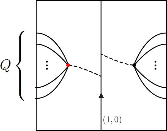
Figure 5: The network corresponding to $Z_{\mathcal{B}/\mathbb{Z}_{P}}(b=0,\widetilde{c}=-\gamma_{2})$.

Therefore we have shown that,

$$Z_{\mathcal{B}/\mathbb{Z}_{P}}(b=-Q\gamma_{1},\widetilde{c}=-\gamma_{2})=\omega^{Q}Z_{\mathcal{B}/\mathbb{Z}_{P}}(b=0,\widetilde{c}=-\gamma_{2}),$$ (3.69)

which is consistent with (3.55) using $\langle\gamma_{1},\gamma_{2}\rangle=1$.

4 Example: $SU(2)_{N}/U(1)_{2N}$ coset CFTs

We demonstrate the $\mathbb{Z}_{N}$ orbifold and parafermionization by examining a well-studied class of coset models with $\mathbb{Z}_{N}$ symmetry,

$${\cal B}=\frac{su(2)_{N}}{u(1)_{2N}}\ .$$ (4.1)

The coset model has the central charge $c=2(N-1)/(N+2)$. Recently, it was shown in [71] that the $\mathbb{Z}_{N}$ symmetry of the model is non-anomalous. For $N=2$, (4.1) can be identified as the Ising model, while for $N=3$ it coincides with the three-state Potts model.

The model (4.1) has the Hilbert space that decomposes into finitely many modules of its chiral algebra. For a given $N$, the chiral algebra allows chiral primaries of weight

$$h_{l,m}=\frac{l(l+2)}{4(N+2)}-\frac{m^{2}}{4N^{2}}\ .$$ (4.2)

where $0\leq l\leq N$ and $|m|\leq l$. The torus partition function of the coset model can be described as

$$Z_{\cal B}=\sum_{l,m}\Big{|}\chi_{l,m}(\tau)\Big{|}^{2}\ ,$$ (4.3)

where $\chi_{l,m}(\tau)$ refers to the conformal character for the chiral primary of weight $h_{l,m}$ (4.2). Since the chiral primaries are subject to various identification

$$\chi_{l,m}(\tau)=\chi_{l,-m}(\tau)=\chi_{l,m+2N}(\tau)=\chi_{N-l,N+m}(\tau)\ ,$$

$$\chi_{l,m}(\tau)=0\quad\text{ if }\quad m-l\in 2\mathbb{Z}\ ,$$ (4.4)

the summation in (4.3) runs over the set

$$\{(l,m)|0\leq l\leq N,-l+2\leq m\leq l,l-m\in 2\mathbb{Z}\}\ .$$ (4.5)

In other words, the coset model ${\cal B}$ has $N(N+1)/2$ independent primary operators.

Turning on the background $\mathbb{Z}_{N}$ gauge field $a=(a_{1},a_{2})$, the partition function $Z_{\cal B}$ becomes

$$Z_{\mathcal{B}}[a_{1},a_{2}]=\frac{1}{2}\sum_{l=0}^{N}\sum_{m=-N+1}^{N}\omega^{(m+a_{1})a_{2}}\chi_{l,m+2a_{1}}(\tau)\chi^{*}_{l,m}(\bar{\tau})\ .$$ (4.6)

Here, we used the $\mathbb{Z}_{N}$ action on each character

$$\chi_{l,m}(\tau)\to e^{\frac{2\pi im}{N}}\chi_{l,m}(\tau)\ ,$$ (4.7)

and the explicit modular $S$-matrix

$$S_{l,m;k,n}=\frac{2}{\sqrt{N(N+2)}}e^{2\pi i\frac{mn}{2N}}\sin{\Big{(}\pi\frac{(l+1)(k+1)}{N+2}\Big{)}}\ ,$$ (4.8)

to express the twisted partition function $Z_{\cal B}[a_{1},a_{2}]$ into the above simple form . We can also see that $T$ and $S$ transformations rotate the twisted partition function in a covariant manner. More precisely, under $T$-transformation, one can show that

$$Z_{\cal B}[a_{1},a_{2}+a_{1}:\tau+1] =\frac{1}{2}\sum_{l=0}^{N}\sum_{m=-N+1}^{N}\omega^{(m+a_{1})(a_{2}+a_{1})}\omega^{-a_{1}(m+a_{1})}\chi_{l,m+2a_{1}}(\tau)\chi^{*}_{l,m}(\bar{\tau})\ ,$$

$$=Z_{\cal B}[a_{1},a_{2}:\tau]\ .$$ (4.9)

On the other hand, the $S$-transformation of the twisted partition function is

$$Z_{\cal B}[a_{2},-a_{1}:-1/\tau]=\frac{1}{2}\sum_{l^{\prime},l^{\prime\prime}=0}^{N}\sum_{m^{\prime},m^{\prime\prime}=-N+1}^{N}c_{l^{\prime},m^{\prime};l^{\prime\prime},m^{\prime\prime}}\chi_{l^{\prime},m^{\prime}}(\tau)\chi^{*}_{l^{\prime\prime};m^{\prime\prime}}(\bar{\tau})$$ (4.10)

with

$$c_{l^{\prime},m^{\prime};l^{\prime\prime},m^{\prime\prime}} =\sum_{l=0}^{N}\sum_{m=-N+1}^{N}\frac{\omega^{-(m+a_{2})a_{1}+\frac{(m+2a_{2})m^{\prime}-mm^{\prime\prime}}{2}}}{N(N+2)}\sin\frac{\pi(l+1)(l^{\prime}+1)}{N+2}\sin\frac{\pi(l+1)(l^{\prime\prime}+1)}{N+2}\ .$$

Since summing over $l$ forces $l^{\prime}=l^{\prime\prime}$ while the sum over $m$ vanishes unless $m^{\prime}=m^{\prime\prime}+2a_{1}$, one obtains

$$c_{l^{\prime},m^{\prime};l^{\prime\prime},m^{\prime\prime}}=\omega^{-a_{1}a_{2}+a_{2}(m^{\prime\prime}+2a1)}\delta_{l^{\prime},l^{\prime\prime}}\delta_{m^{\prime},m^{\prime\prime}+2a_{1}}\ ,$$ (4.11)

and thus

$$Z_{\cal B}[a_{2},-a_{1}:-1/\tau]=Z_{\cal B}[a_{1},a_{2}:\tau]\ .$$ (4.12)

It is well-known that the Ising model is self-dual under the Krammers-Wannier duality. Similarly, the $\mathbb{Z}_{N}$ gauging maps the coset model (4.1) to itself

$$\widetilde{\cal B}\equiv{\cal B}/\mathbb{Z}_{N}\simeq{\cal B}\ .$$ (4.13)

To see this, let us recall that the partition function of the orbifold $\widetilde{\cal B}$ coupled to the background field is

$$Z_{{\cal B}/\mathbb{Z}_{N}}[\tilde{a}_{1},\tilde{a}_{2}] =\frac{1}{N}\sum_{a_{1},a_{2}}\omega^{\tilde{a}_{1}a_{2}-\tilde{a}_{2}a_{1}}Z_{\cal B}[a_{1},a_{2}]$$ (4.14)

$$=\frac{1}{2N}\sum_{l=0}^{N}\sum_{m=-N+1}^{N}\sum_{a_{1},a_{2}}\omega^{(m+a_{1})a_{2}-(a_{1}\tilde{a}_{2}-a_{2}\tilde{a}_{1})}\chi_{l,m+2a_{1}}(\tau)\chi^{*}_{l,m}(\bar{\tau})\ ,$$

where we used (4.6) for the second equality. Since the sum over the $\mathbb{Z}_{N}$ holonomy $a_{2}$ is identically zero unless $a_{1}=-(\tilde{a}_{1}+m)$, the above expression can be simplified as follows

$$Z_{{\cal B}/\mathbb{Z}_{N}}[\tilde{a}_{1},\tilde{a}_{2}] =\frac{1}{2}\sum_{l=0}^{N}\sum_{m=-N+1}^{N}\omega^{(\tilde{a}_{1}+m)\tilde{a}_{2}}\chi_{l,-m-2\tilde{a}_{1}}(\tau)\chi^{*}_{l,m}(\bar{\tau})\ .$$ (4.15)

It perfectly matches with $Z_{\cal B}[a]$ with $(a_{1},a_{2})=(\tilde{a}_{1},\tilde{a}_{2})$ due to the charge conjugation symmetry $\chi_{l,m}(\tau)=\chi_{l,-m}(\tau)$.

Let us finally move onto the parafermionic theories dual to the coset models. Based on the parafermionization (3.20), one can obtain the torus partition function of our interest

$$Z_{\cal PF}[s_{1},s_{2};k] =\frac{1}{N}\sum_{a_{1},a_{2}}\omega^{k\text{Arf}_{N}(s+a)}Z_{\cal B}[a_{1},a_{2}]\ ,$$ (4.16)

$$=\frac{1}{2N}\sum_{l=0}^{N}\sum_{m=-N+1}^{N}\sum_{a_{1},a_{2}}\omega^{k(s_{1}+a_{1})(s_{2}+a_{2})+(m+a_{1})a_{2}}\chi_{l,m+2a_{1}}(\tau)\chi^{*}_{l,m}(\bar{\tau})\ ,$$

where $Z_{\cal B}[a_{1},a_{2}]$ is given by (4.6). It can be further massaged into a simpler expression

$$Z_{\cal PF}[s_{1},s_{2};k]=\frac{1}{2}\sum_{l=0}^{N}\sum_{a_{1}}\omega^{k(s_{1}+a_{1})s_{2}}\Big{[} \chi_{l,ks_{1}+(k-1)a_{1}}(\tau)\chi^{*}_{l,ks_{1}+(k+1)a_{1}}(\bar{\tau})$$

$$+ \chi_{l,ks_{1}+(k-1)a_{1}+N}(\tau)\chi^{*}_{l,ks_{1}+(k+1)a_{1}+N}(\bar{\tau})\Big{]}\ .$$ (4.17)

Note that, for $k=1$, (4) reduces to the torus partition function proposed in [57]. In this case the $\mathbb{Z}_{N}$ duality web in Table 3.1 follows from the identity

$$Z_{\cal PF}[-ks_{1},ks_{2};1/k]=\omega^{-ks_{1}s_{2}}Z_{\cal PF}[s_{1},s_{2};k]\ .$$ (4.18)

Acknowledgements

We would like to thank Chi-Ming Chang, Jin Chen and Kimyeong Lee for helpful discussions. We also thank Chi-Ming Chang for comments on the draft. ZD thanks Fudan University, Shanghai for hospitality where part of this project was carried out. The main result of this work was presented by QJ at the 4th National Workshop on Fields and Strings held in Nanjing, and QJ is grateful to the audience for feedback. ZD, QJ, and SL are supported by KIAS Grant PG076902, PG080802 and PG056502.

Appendix A Operators defining parafermionic states

In this appendix, we will give a systematic discussion about operators $U_{Pf;k}[\Gamma]$ defined in (3.14). We begin with the general sets of operators labeled by a pair $(k,l)$,

$$U_{Pf;k,l}[\Gamma]=U[m\Gamma_{1}]^{-k}U[n\Gamma_{2}]^{k}\widetilde{U}[m\Gamma_{1}]^{l}\widetilde{U}[n\Gamma_{2}]^{l},$$ (A.1)

where the operators in (3.14) corresponds to $l=1$. They satisfy,

$$U_{Pf;k,l}[\Gamma]U_{Pf;k,l}[\Gamma^{\prime}]$$

$$= U[m\Gamma_{1}]^{-k}U[n\Gamma_{2}]^{k}\widetilde{U}[m\Gamma_{1}]^{l}\widetilde{U}[n\Gamma_{2}]^{l}U[m^{\prime}\Gamma_{1}]^{-k}U[n^{\prime}\Gamma_{2}]^{k}\widetilde{U}[m^{\prime}\Gamma_{1}]^{l}\widetilde{U}[n^{\prime}\Gamma_{2}]$$

$$= U[(m+m^{\prime})\Gamma_{1}]^{-k}U[(n+n^{\prime})\Gamma_{2}]^{k}\widetilde{U}[(m+m^{\prime})\Gamma_{1}]^{l}\widetilde{U}[(n+n^{\prime})\Gamma_{2}]^{l}\omega^{kl\langle m\gamma_{1}+n\gamma_{2},m^{\prime}\gamma_{1}-n^{\prime}\gamma_{2}\rangle}$$

$$= U_{Pf;k,l}[\Gamma+\Gamma^{\prime}]\omega^{kl(\gamma,\gamma^{\prime})},$$ (A.2)

where $(*,*)$ is the symmetric pairing defined as $(a,b)=a_{1}b_{2}+a_{2}b_{1}$. The operators labeled by the same pair $(k,l)$ commute with each other. For operators with different $(k,l)$-pair, one has the commutation relation,

$$U_{Pf;l,k}[\Gamma]U_{Pf;l^{\prime},k^{\prime}}[\Gamma^{\prime}]$$

$$= U[m\Gamma_{1}]^{-k}U[n\Gamma_{2}]^{k}\widetilde{U}[m\Gamma_{1}]^{l}\widetilde{U}[n\Gamma_{2}]^{l}U[m^{\prime}\Gamma_{1}]^{-k^{\prime}}U[n^{\prime}\Gamma_{2}]^{k^{\prime}}\widetilde{U}[m^{\prime}\Gamma_{1}]^{l^{\prime}}\widetilde{U}[n^{\prime}\Gamma_{2}]^{l^{\prime}}$$

$$= U[m^{\prime}\Gamma_{1}]^{-k^{\prime}}U[n^{\prime}\Gamma_{2}]^{k^{\prime}}\left(U[m\Gamma_{1}]^{-k}U[n\Gamma_{2}]^{k}\widetilde{U}[m\Gamma_{1}]^{l}\widetilde{U}[n\Gamma_{2}]^{l}\right)\widetilde{U}[m^{\prime}\Gamma_{1}]^{l^{\prime}}\widetilde{U}[n^{\prime}\Gamma_{2}]^{l^{\prime}}\omega^{lk^{\prime}(\gamma,\gamma^{\prime})}$$

$$= U[m^{\prime}\Gamma_{1}]^{-k^{\prime}}U[n^{\prime}\Gamma_{2}]^{k^{\prime}}\widetilde{U}[m^{\prime}\Gamma_{1}]^{l^{\prime}}\widetilde{U}[n^{\prime}\Gamma_{2}]^{l^{\prime}}U[m\Gamma_{1}]^{-k}U[n\Gamma_{2}]^{k}\widetilde{U}[m\Gamma_{1}]^{l}\widetilde{U}[n\Gamma_{2}]^{l}\omega^{(lk^{\prime}-l^{\prime}k)(\gamma,\gamma^{\prime})}$$

$$= U_{Pf;l^{\prime},k^{\prime}}[\Gamma^{\prime}]U_{Pf;l,k}[\Gamma]\omega^{(lk^{\prime}-l^{\prime}k)(\gamma,\gamma^{\prime})}.$$ (A.3)

They are commuting only if $lk^{\prime}-l^{\prime}k=0$, which is equivalent to $k^{\prime}=\lambda k,l^{\prime}=\lambda l$ for some non-zero $\lambda$. If $\lambda$ is coprime with $N$, the operators $U_{Pf;k^{\prime},l^{\prime}}$ is equivalent to $U_{Pf;k,l}$ up to rescaling of $\Gamma$, otherwise it is a subalgebra of $U_{Pf;k,l}$.

There are three cases depending on whether $k$ and $l$ are coprime with $N$:

• If $l$ is coprime with $N$, then one can choose a representative $l=1$ up to rescaling of $\Gamma$,

  $$U_{Pf;k,1}[\Gamma]=U[m\Gamma_{1}]^{-k}U[n\Gamma_{2}]^{k}\widetilde{U}[m\Gamma_{1}]\widetilde{U}[n\Gamma_{2}],$$ (A.4)

  which is the operators defined in (3.14).

• If $k$ is coprime with $N$, then we can set $k=1$ and get,

  $$U_{Pf;1,l}[\Gamma]=U[m\Gamma_{1}]^{-1}U[n\Gamma_{2}]\widetilde{U}[m\Gamma_{1}]^{l}\widetilde{U}[n\Gamma_{2}]^{l}.$$ (A.5)

  This kind of operator is related to the parafermionic operator (3.61) when we discuss partial gauging.

• Both $k$ and $l$ are not coprime with $N$. We did not consider this case in the paper so we omit the discussion here.

References

• [1] D. Gaiotto, A. Kapustin, N. Seiberg and B. Willett, Generalized Global Symmetries, JHEP 02 (2015) 172 [1412.5148].
• [2] F. Albertini, M. Del Zotto, I.n. García Etxebarria and S.S. Hosseini, Higher Form Symmetries and M-theory, JHEP 12 (2020) 203 [2005.12831].
• [3] D.R. Morrison, S. Schafer-Nameki and B. Willett, Higher-Form Symmetries in 5d, JHEP 09 (2020) 024 [2005.12296].
• [4] C. Córdova, T.T. Dumitrescu and K. Intriligator, Exploring 2-Group Global Symmetries, JHEP 02 (2019) 184 [1802.04790].
• [5] C. Cordova, T.T. Dumitrescu and K. Intriligator, 2-Group Global Symmetries and Anomalies in Six-Dimensional Quantum Field Theories, JHEP 04 (2021) 252 [2009.00138].
• [6] L. Bhardwaj and S. Schäfer-Nameki, Higher-form symmetries of 6d and 5d theories, JHEP 02 (2021) 159 [2008.09600].
• [7] J. Tian and Y.-N. Wang, 5D and 6D SCFTs from $\mathbb{C}^{3}$ orbifolds, SciPost Phys. 12 (2022) 127 [2110.15129].
• [8] M. Del Zotto, I.n. García Etxebarria and S. Schafer-Nameki, 2-Group Symmetries and M-Theory, SciPost Phys. 13 (2022) 105 [2203.10097].
• [9] M. Del Zotto, J.J. Heckman, S.N. Meynet, R. Moscrop and H.Y. Zhang, Higher symmetries of 5D orbifold SCFTs, Phys. Rev. D 106 (2022) 046010 [2201.08372].
• [10] Y.-N. Wang and Y. Zhang, Fermionic Higher-form Symmetries, 2303.12633.
• [11] L. Bhardwaj and Y. Tachikawa, On finite symmetries and their gauging in two dimensions, JHEP 03 (2018) 189 [1704.02330].
• [12] C.-M. Chang, Y.-H. Lin, S.-H. Shao, Y. Wang and X. Yin, Topological Defect Lines and Renormalization Group Flows in Two Dimensions, JHEP 01 (2019) 026 [1802.04445].
• [13] R. Thorngren and Y. Wang, Fusion Category Symmetry I: Anomaly In-Flow and Gapped Phases, 1912.02817.
• [14] Z. Komargodski, K. Ohmori, K. Roumpedakis and S. Seifnashri, Symmetries and strings of adjoint QCD2, JHEP 03 (2021) 103 [2008.07567].
• [15] R. Thorngren and Y. Wang, Fusion Category Symmetry II: Categoriosities at $c$ = 1 and Beyond, 2106.12577.
• [16] Y. Choi, C. Cordova, P.-S. Hsin, H.T. Lam and S.-H. Shao, Noninvertible duality defects in 3+1 dimensions, Phys. Rev. D 105 (2022) 125016 [2111.01139].
• [17] J. Kaidi, K. Ohmori and Y. Zheng, Kramers-Wannier-like Duality Defects in (3+1)D Gauge Theories, Phys. Rev. Lett. 128 (2022) 111601 [2111.01141].
• [18] Y. Choi, C. Cordova, P.-S. Hsin, H.T. Lam and S.-H. Shao, Non-invertible Condensation, Duality, and Triality Defects in 3+1 Dimensions, 2204.09025.
• [19] C. Cordova and K. Ohmori, Noninvertible Chiral Symmetry and Exponential Hierarchies, Phys. Rev. X 13 (2023) 011034 [2205.06243].
• [20] Y. Choi, H.T. Lam and S.-H. Shao, Noninvertible Global Symmetries in the Standard Model, Phys. Rev. Lett. 129 (2022) 161601 [2205.05086].
• [21] C.-M. Chang, J. Chen, K. Kikuchi and F. Xu, Topological Defect Lines in Two Dimensional Fermionic CFTs, 2208.02757.
• [22] V. Bashmakov, M. Del Zotto, A. Hasan and J. Kaidi, Non-invertible symmetries of class S theories, JHEP 05 (2023) 225 [2211.05138].
• [23] N. Seiberg, Field Theories With a Vector Global Symmetry, SciPost Phys. 8 (2020) 050 [1909.10544].
• [24] N. Seiberg and S.-H. Shao, Exotic Symmetries, Duality, and Fractons in 2+1-Dimensional Quantum Field Theory, SciPost Phys. 10 (2021) 027 [2003.10466].
• [25] N. Seiberg and S.-H. Shao, Exotic $U(1)$ Symmetries, Duality, and Fractons in 3+1-Dimensional Quantum Field Theory, SciPost Phys. 9 (2020) 046 [2004.00015].
• [26] N. Seiberg and S.-H. Shao, Exotic $\mathbb{Z}_{N}$ symmetries, duality, and fractons in 3+1-dimensional quantum field theory, SciPost Phys. 10 (2021) 003 [2004.06115].
• [27] S. Yamaguchi, Gapless edge modes in (4+1)-dimensional topologically massive tensor gauge theory and anomaly inflow for subsystem symmetry, PTEP 2022 (2022) 033B08 [2110.12861].
• [28] C. Stahl, E. Lake and R. Nandkishore, Spontaneous breaking of multipole symmetries, Phys. Rev. B 105 (2022) 155107 [2111.08041].
• [29] P. Gorantla, H.T. Lam, N. Seiberg and S.-H. Shao, Global dipole symmetry, compact Lifshitz theory, tensor gauge theory, and fractons, Phys. Rev. B 106 (2022) 045112 [2201.10589].
• [30] H. Katsura and Y. Nakayama, Spontaneously broken supersymmetric fracton phases with fermionic subsystem symmetries, JHEP 08 (2022) 072 [2204.01924].
• [31] P. Gorantla, H.T. Lam, N. Seiberg and S.-H. Shao, 2+1d Compact Lifshitz Theory, Tensor Gauge Theory, and Fractons, 2209.10030.
• [32] S. Yamaguchi, SL (2, $\mathbb{Z}$) action on quantum field theories with U(1) subsystem symmetry, PTEP 2023 (2023) 023B06 [2208.13193].
• [33] W. Cao, M. Yamazaki and Y. Zheng, Boson-fermion duality with subsystem symmetry, Phys. Rev. B 106 (2022) 075150 [2206.02727].
• [34] W. Cao, L. Li, M. Yamazaki and Y. Zheng, Subsystem Non-Invertible Symmetry Operators and Defects, 2304.09886.
• [35] C. Cordova, T.T. Dumitrescu, K. Intriligator and S.-H. Shao, Snowmass White Paper: Generalized Symmetries in Quantum Field Theory and Beyond, in Snowmass 2021, 5, 2022 [2205.09545].
• [36] S. Schafer-Nameki, ICTP Lectures on (Non-)Invertible Generalized Symmetries, 2305.18296.
• [37] T.D. Brennan and S. Hong, Introduction to Generalized Global Symmetries in QFT and Particle Physics, 2306.00912.
• [38] L. Bhardwaj, L.E. Bottini, L. Fraser-Taliente, L. Gladden, D.S.W. Gould, A. Platschorre et al., Lectures on Generalized Symmetries, 2307.07547.
• [39] R. Luo, Q.-R. Wang and Y.-N. Wang, Lecture Notes on Generalized Symmetries and Applications, 7, 2023 [2307.09215].
• [40] D. Gaiotto and J. Kulp, Orbifold groupoids, 2008.05960.
• [41] F. Apruzzi, F. Bonetti, I.n.G. Etxebarria, S.S. Hosseini and S. Schafer-Nameki, Symmetry TFTs from String Theory, 2112.02092.
• [42] Y.-H. Lin, M. Okada, S. Seifnashri and Y. Tachikawa, Asymptotic density of states in 2d CFTs with non-invertible symmetries, JHEP 03 (2023) 094 [2208.05495].
• [43] J. Kaidi, K. Ohmori and Y. Zheng, Symmetry TFTs for Non-Invertible Defects, 2209.11062.
• [44] M. van Beest, D.S.W. Gould, S. Schafer-Nameki and Y.-N. Wang, Symmetry TFTs for 3d QFTs from M-theory, JHEP 02 (2023) 226 [2210.03703].
• [45] J. Kaidi, E. Nardoni, G. Zafrir and Y. Zheng, Symmetry TFTs and Anomalies of Non-Invertible Symmetries, 2301.07112.
• [46] L. Bhardwaj and S. Schafer-Nameki, Generalized Charges, Part II: Non-Invertible Symmetries and the Symmetry TFT, 2305.17159.
• [47] T. Bartsch, M. Bullimore and A. Grigoletto, Representation theory for categorical symmetries, 2305.17165.
• [48] J. Chen, W. Cui, B. Haghighat and Y.-N. Wang, SymTFTs and Duality Defects from 6d SCFTs on 4-manifolds, 2305.09734.
• [49] D.S. Freed, G.W. Moore and C. Teleman, Topological symmetry in quantum field theory, 2209.07471.
• [50] D. Gaiotto and A. Kapustin, Spin TQFTs and fermionic phases of matter, Int. J. Mod. Phys. A 31 (2016) 1645044 [1505.05856].
• [51] A. Karch, D. Tong and C. Turner, A Web of 2d Dualities: ${\bf Z}_{2}$ Gauge Fields and Arf Invariants, SciPost Phys. 7 (2019) 007 [1902.05550].
• [52] C.-T. Hsieh, Y. Nakayama and Y. Tachikawa, On fermionic minimal models, 2002.12283.
• [53] J. Kulp, Two More Fermionic Minimal Models, 2003.04278.
• [54] E. Fradkin and L.P. Kadanoff, Disorder variables and para-fermions in two-dimensional statistical mechanics, Nuclear Physics B 170 (1980) 1.
• [55] V. Fateev and A. Zamolodchikov, Conformal quantum field theory models in two dimensions having z3 symmetry, Nuclear Physics B 280 (1987) 644.
• [56] D. Gepner and Z. Qiu, Modular invariant partition functions for parafermionic field theories, Nuclear Physics B 285 (1987) 423.
• [57] Y. Yao and A. Furusaki, Parafermionization, bosonization, and critical parafermionic theories, JHEP 04 (2021) 285 [2012.07529].
• [58] I.M. Burbano, J. Kulp and J. Neuser, Duality defects in E8, JHEP 10 (2022) 186 [2112.14323].
• [59] B. Haghighat and Y. Sun, Topological Defect Lines in bosonized Parafermionic CFTs, 2306.16555.
• [60] Z. Duan, Q. Jia and S. Lee. work in progress.
• [61] Y. Tachikawa, TASI 2019 Lectures, https://member.ipmu.jp/yuji.tachikawa/lectures/2019-top-anom.
• [62] J. Chen, B. Haghighat and Q.-R. Wang, Para-fusion Category and Topological Defect Lines in $\mathbb{Z}_{N}$-parafermionic CFTs, 2309.01914.
• [63] M.F. Atiyah, Riemann surfaces and spin structures, Annales scientifiques de l’École Normale Supérieure Ser. 4, 4 (1971) 47.
• [64] E. Witten, Quantum Field Theory and the Jones Polynomial, Commun. Math. Phys. 121 (1989) 351.
• [65] L. Kong, Anyon condensation and tensor categories, Nuclear Physics B 886 (2014) 436.
• [66] D. Aasen, E. Lake and K. Walker, Fermion condensation and super pivotal categories, J. Math. Phys. 60 (2019) 121901 [1709.01941].
• [67] I. Runkel and L. Szegedy, Topological field theory on r-spin surfaces and the Arf-invariant, J. Math. Phys. 62 (2021) 102302 [1802.09978].
• [68] J.-B. Bae, Z. Duan, K. Lee, S. Lee and M. Sarkis, Fermionic Rational Conformal Field Theories and Modular Linear Differential Equations, Progress of Theoretical and Experimental Physics (ptab033, 2021) [2010.12392].
• [69] J.-B. Bae, Z. Duan, K. Lee, S. Lee and M. Sarkis, Bootstrapping fermionic rational CFTs with three characters, JHEP 01 (2022) 089 [2108.01647].
• [70] Z. Duan, K. Lee, S. Lee and L. Li, On classification of fermionic rational conformal field theories, JHEP 02 (2023) 079 [2210.06805].
• [71] Y.-H. Lin and S.-H. Shao, $\mathbb{Z}_{N}$ symmetries, anomalies, and the modular bootstrap, Phys. Rev. D 103 (2021) 125001 [2101.08343].