Abstract

We discuss energy conditions and quasinormal modes for scalar perturbations of regular charged black holes within the framework of General Relativity coupled to non-linear electrodynamics. The frequencies are computed numerically adopting the WKB method, while in the eikonal limit an analytic expression for the spectra is obtained. The impact of the electric charge, the angular degree, and the overtone number on the spectra is investigated in detail. We find that all frequencies are characterized by a negative imaginary part, and that each type of energy conditions imply a different quasinormal spectrum.

Key words: Static regular black hole; energy conditions; non-linear electrodynamics; quasi-normal modes.

1 Introduction

Realistic black holes are not isolated in Nature. Instead, they are in constant interaction with their environment. When a black hole is perturbed, the geometry of space-time undergoes damped oscillations. How a system responds to small perturbations has always been important in physics. The work of [1] marked the birth of black hole perturbations, it was later extended by [2, 3, 4, 5, 6], while the state-of-the art in black hole perturbations is summarized in the comprehensive review of Chandrasekhar’s monograph [7]. Quasi-normal (QN) frequencies are complex numbers, with a non-vanishing imaginary part, that encode the information on how black holes relax after the perturbation has been applied. They depend on the geometry itself as well as the type of the perturbation (scalar, Dirac, vector (electromagnetic), tensor (gravitational)). As they do not depend on the initial conditions, QN modes (QNMs) carry unique information about black holes. Black hole perturbation theory and QNMs of black holes are relevant during the ringdown phase of binaries, in which after the merging of two black holes a new, distorted object is formed, while at the same time the geometry of space-time undergoes damped oscillations due to the emission of gravitational waves.

Given the interest in gravitational wave astronomy and in QNMs of black holes, it would be interesting to see what kind of QN spectra are expected from regular electrically charged black holes in non-linear electrodynamics. In the present work we propose to compute QNMs for scalar perturbations of black hole solutions with a net electric charge within four distinct non-linear electrodynamics (NLE) models fulfilling different energy conditions.

There are certain static black hole solutions that have an event horizon and whose metric and curvature invariants $R$, $R_{\mu\nu}R^{\mu\nu}$, $R_{\kappa\lambda\mu\nu}R^{\kappa\lambda\mu\nu}$ do not present singularities in the whole interval of the radial coordinate $r$. Such solutions are known as regular (or non-singular) black holes. Some of these regular solutions [8, 9, 10, 11, 12, 13, 14] have no electric or magnetic charge, they depend on the mass of the black hole and some extra parameter and asymptotically behave as the Schwarzschild solution. Other solutions have electric (or magnetic) charge, but in this group are those that do not behave like the Reissner-Nordstrom solution in the limit of weak fields, for example the Bardeen solution [15], which can be obtained from a nonlinear electrodynamics of a magnetic source [16] or of a electric source [17]. The Hayward solution given in Ref. [10] can also be considered as such a charged solution of this type [18] (see also other examples given in this same reference). A large number of regular black hole solutions have been found using nonlinear electromagnetic sources, which in the weak field limit behave like the Reissner-Nordstrom solution, for example [19, 20, 21, 22, 23]. For recent literature about regular black holes see for instance [24, 25, 26, 27, 28, 29].

The energy conditions are the constraints for the energy-momentum tensor $T^{\mu\nu}$ of a theory of gravity [30]. The standard acceptable conditions assumed for the energy-momentum tensor are: weak energy condition (WEC), dominant energy condition (DEC), null energy condition (NEC), and strong energy condition (SEC) (see Refs. [30, 31, 32]). If $\xi_{\mu}$ and $k_{\mu}$ are arbitrary timelike and null vectors, respectively, then the conditions for the energy-momentum tensor are expressed with the following inequalities

$$T^{\mu\nu}\xi_{\mu}\xi_{\nu}\geq 0\,\,\,\,\,\,\mbox{(WEC)}.$$ (1)

$$T^{\mu\nu}\xi_{\mu}\xi_{\nu}\geq 0\mbox{ and }T^{\mu\nu}\xi_{\mu}\mbox{ is a non-spacelike vector}\,\,\,\,\,\,\mbox{(DEC)}.$$ (2)

$$T^{\mu\nu}k_{\mu}k_{\nu}\geq 0\,\,\,\,\,\,\mbox{(NEC)}.$$ (3)

$$T^{\mu\nu}\xi_{\mu}\xi_{\nu}-\frac{1}{2}T^{\mu}_{\,\,\,\mu}\xi^{\nu}\xi_{\nu}\geq 0\,\,\,\,\,\,\mbox{(SEC)}.$$ (4)

The above inequalities imply for a perfect fluid the energy conditions

$$\rho\geq 0,$$ (5)

$$\rho\pm p\geq 0,$$ (6)

$$\rho+3p\geq 0,$$ (7)

where $p,\rho$ are the pressure and the energy density of the fluid, respectively.

The regular black holes violate the SEC somewhere inside the event horizon [33]. However, a regular black hole could satisfy the NEC or the WEC or the DEC everywhere. Those regular black holes that satisfy the WEC necessarily have asymptotically de Sitter behavior for $r\rightarrow 0$ [34]. The WEC together with the symmetry $T_{\,\,\,0}^{0}=T_{\,\,\,1}^{1}$ for the energy-momentum tensor have been used to obtain new solutions of regular black holes [18, 35] and without it having been a requirement that these solutions also satisfy the DEC everywhere.

Regular black hole solutions can be classified either by the energy conditions that they satisfy or by the way in which they do not satisfy these energy conditions.

In the present article our work is organized as follows: After this introductory section, in section 2 we summarize the field equations for Einstein gravity coupled to non-linear Electrodynamics. In the third section we discuss energy conditions, while in section 4 the stability of the BH solutions analyzed here is discussed. Finally, in the fifth section we compute the QN spectra, and we conclude our work in section 6. We adopt the mostly positive metric signature $(-,+,+,+)$, and we work in geometrical units where $G=1=c$.

2 Regular charged black holes

The solutions of charged regular black holes can be obtained from the following action of general relativity coupled with a nonlinear electrodynamics model

$$S=\int d^{4}x\sqrt{-g}\left(\frac{R}{16\pi}-\mathcal{L}(\mathcal{F})\right)\,,$$ (8)

where $g$ is the determinant of the metric tensor, $R$ is the Ricci scalar, and $\mathcal{L}(\mathcal{F})$ is the Lagrangian that depends on the Lorentz invariant $\mathcal{F}=F^{\mu\nu}F_{\mu\nu}/4$. In these theories the electrodynamic model is expressed by a Hamiltonian function $\mathcal{H}(\mathcal{P})$ and fields $P^{\mu\nu}$ instead of $\mathcal{L}(\mathcal{F})$ and the fields of the electromagnetic tensor $F^{\mu\nu}$, but which are related by the Legendre transformation $\mathcal{L}=P_{\mu\nu}F^{\mu\nu}-\mathcal{H}$.

Here we adopt the following most general form of a static line element with spherical symmetry

$$ds^{2}=-f(r)dt^{2}+f(r)^{-1}dr^{2}+r^{2}(d\theta^{2}+\sin^{2}\theta d^{2}\phi)\,,$$ (9)

where the metric function is given by

$$f(r)=1-\frac{2m(r)}{r}\,,$$ (10)

and $m(r)$ is the mass function that depends on the mass $M$, the electric charge $q$ of the black hole as well as the radial coordinate $r$.

Computing the variation of the action (8) allows us to obtain the Einstein field equations

$$G_{\mu\nu}=R_{\mu\nu}-\frac{1}{2}Rg_{\mu\nu}=8\pi T_{\mu\nu}\,,$$ (11)

and

$$\nabla_{\mu}\left(F^{\mu\nu}\frac{d\mathcal{L}}{d\mathcal{F}}\right)=0\,.$$ (12)

Here

$$T_{\mu\nu}=\frac{1}{4\pi}\left(g_{\mu\nu}\mathcal{L}(\mathcal{F})-F_{\mu\alpha}F_{\nu}^{\,\alpha}\frac{d\mathcal{L}}{d\mathcal{F}}\right)\,.$$ (13)

From these last three equations we can obtain a general expression for the electric field $\mathbf{E}=E(r)\hat{r}$ in terms of the mass function

$$E(r)=\frac{r}{2q}\left(\frac{2}{r}\frac{dm(r)}{dr}-\frac{d^{2}m(r)}{dr^{2}}\right)\,.$$ (14)

3 Energy conditions and regular charged black holes

We can conveniently express the energy conditions given above, if we note that from Eqs. (9) and (10) we obtain

$$G^{0}_{\,\,0}=G^{1}_{\,\,1}=\frac{1}{r^{2}}\left(-1+f(r)+\frac{df(r)}{dr}\right)=-2\frac{dm(r)}{dr}\ ,$$ (15)

$$G^{2}_{\,\,2}=G^{3}_{\,\,3}=\frac{1}{r}\frac{df(r)}{dr}+\frac{1}{2}\frac{d^{2}f(r)}{dr^{2}}=-\frac{1}{r}\frac{d^{2}m(r)}{dr^{2}}\ ,$$ (16)

and therefore the field equations (11) imply for the stress-energy tensor

$$T^{0}_{\,\,0}=T^{1}_{\,\,1}=-\frac{2}{8\pi r^{2}}\frac{dm(r)}{dr}\ ,$$ (17)

$$T^{2}_{\,\,2}=T^{3}_{\,\,3}=-\frac{1}{8\pi r}\frac{d^{2}m(r)}{dr^{2}}\ .$$ (18)

Thus we can write that the WEC requires the following inequalities to be satisfied for all $r$

$$\frac{1}{r^{2}}\frac{dm(r)}{dr}\geq 0\ ,$$ (19)

and

$$\frac{2}{r}\frac{dm(r)}{dr}-\frac{d^{2}m(r)}{dr^{2}}\geq 0\,.$$ (20)

where the first one is equivalent to the condition $\rho\geq 0$ (or $-T_{0}^{0}\geq 0$), while the other one is equivalent to the condition $p+\rho\geq 0$ (or $-T_{0}^{0}+T_{2}^{2}\geq 0$).

Meanwhile, the DEC requires that the two previous inequalities be satisfied along with the following inequality

$$\frac{2}{r}\frac{dm(r)}{dr}+\frac{d^{2}m(r)}{dr^{2}}\geq 0\,.$$ (21)

The NEC requires that only inequality (20) be satisfied.

Note that the DEC implies the WEC and in turn the WEC implies the NEC. Also note that from the expression (20) obtained for the electric field, if the WEC (or NEC) is violated on some interval, then on this same interval the electric field is negative (where the electric charge is $|q|$).

Based on the energy conditions mentioned above, we can classify static regular black holes into three types:

1. Those who satisfy the DEC everywhere and therefore also the WEC (and the NEC).

2. Those who satisfy the WEC everywhere, but do not satisfy the DEC somewhere.

3. Those who do not satisfy the WEC somewhere in $r$. In terms of the inequalities given above, we see that there are two different ways of not satisfying it. In both cases inequality (20) is not fulfilled, but in one case inequality (21) is fulfilled and in the other case is not.

Below, we consider an example of a regular black hole of each type, we study the intervals where it does not satisfy some energy condition. Based on inequalities (20) and (21), together with considering that the solutions that we will analyze satisfy inequality (19), and since in general the analysis can be performed only numerically, we define the following functions to find the interval in that a black hole solution violates some of the energy conditions

$$g(r)=\frac{2}{r}\frac{dm(r)}{dr}-\frac{d^{2}m(r)}{dr^{2}}\,,$$ (22)

$$h(r)=\frac{2}{r}\frac{dm(r)}{dr}+\frac{d^{2}m(r)}{dr^{2}}\,.$$ (23)

3.1 Case I: solution that satisfies the DEC everywhere

The first model is taken from Ref. [18], which we call case I in this article. The metric function in this model is

$$f_{I}(r)=1-\frac{2M}{r}\left(1-\frac{1}{\left(1+\left(\frac{2Mr}{q^{2}}\right)^{3}\right)^{1/3}}\right)\,.$$ (24)

This metric function asymptotically behaves as the Reissner-Nordström solution. In the limit $r\rightarrow 0$ behaves as a de Sitter solution,

$$f_{I}(r)\rightarrow 1-\frac{16M^{4}}{3q^{6}}r^{2}\,.$$ (25)

The extreme black hole occurs when $q_{ext}=1.0257M$.

In this case by construction the black hole solution satisfies the WEC in all $r$ and, moreover, also satisfies the DEC for $0<q\leq q_{ext}$ [18].

3.2 Case II: ABG solution

The second model is the ABG [19] solution, whose metric function is given by

$$f_{II}(r)=1-\frac{2M}{r}\left(\frac{r^{3}}{(r^{2}+q^{2})^{3/2}}-\frac{q^{2}r^{3}}{2M(r^{2}+q^{2})^{2}}\right)\,.$$ (26)

This model also behaves as the Reissner-Nordström solution in the limit of weak fields, while for $r\rightarrow 0$ asymptotically it is

$$f_{II}(r)\rightarrow 1-\frac{(2M-q)}{q^{3}}r^{2}\,.$$ (27)

The extremal solution is obtained when $q_{ext}=0.6342M$.

As is known, the ABG solution satisfies the WEC everywhere (i.e. inequality (19) and condition $g(r)>0$ are satisfied for all $r$), however from a value of $r$ to infinity it violates the DEC, since $h(r)<0$, as shown in Fig. (1).

The DEC can be violated from a point that is inside the event horizon or from a point that is outside, to infinity. This is determined by the value of the electric charge of the black hole. In this way, if the electric charge is $q_{0}=0.5727M$ (which determines that the event horizon is at $r_{h0}=1.4288M$) the DEC is violated from the event horizon to infinity. If $q<q_{0}$ the DEC is violated from a point inside the event horizon (which is different from $r_{h0}$). And if $q_{0}<q\leq q_{ext}$ the point lies outside the event horizon.

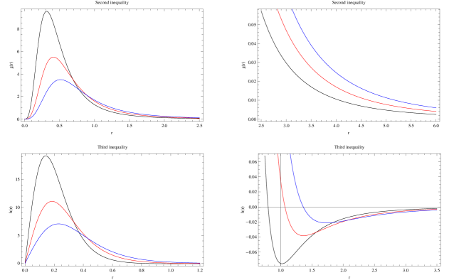
Figure 1: For case II, the functions $g(r)$ and $h(r)$ are represented for $q=0.35M$ (black), $q=0.45M$ (red) and $q=0.55M$ (blue), and $M=1$ in each picture. The figures on the right amplify the scale of the vertical axis. Here the WEC is satisfied everywhere as illustrated in the two pictures on the top, i.e. the second inequality given by Eq. (20) is satisfied everywhere. However, inequality (21) does not hold in an interval from $r<r_{h}$ to infinity, that is, the DEC is violated in this region, as can be seen in the fourth figure, where the curves cross towards down the $r$ axis.

3.3 Case III: solution with exponential

The following model is one of the solutions proposed in Ref. [23], and whose metric function is written as

$$f_{III}(r)=1-\frac{2M}{r}\exp\left(-\frac{q^{2}}{2Mr}\right)\,,$$ (28)

which behaves like the Reissner-Nordström solution in the limit $r\rightarrow\infty$. The extreme case is obtained when $q_{ext}=1.2131M$ and $r_{h}=0.7355M$.

This regular black hole solution violates the WEC (or $g(r)<0$) and therefore also violates the DEC, in a region that is inside the event horizon, as illustrated in Fig. (2) for three different electric charge values $q$. However, it can be shown that this conclusion holds for all $0<q\leq q_{ext}$. Notice also in the bottom two pictures of Fig. (2) that inequality (21) holds everywhere.

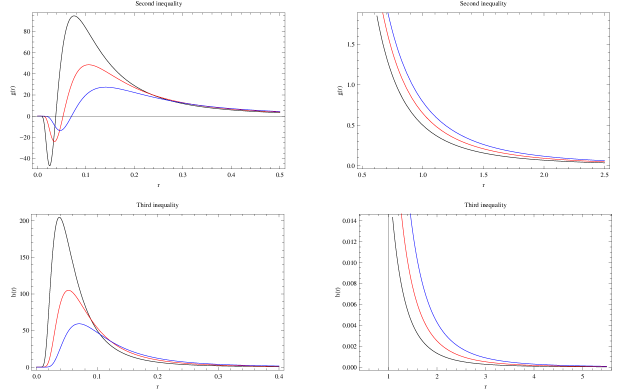
Figure 2: Case III. The functions $g(r)$ and $h(r)$ are represented for $q=0.55M$ (black), $q=0.65M$ (red) and $q=0.75M$ (blue), and $M=$1 in each picture. Here the condition (20) is not satisfied in a region inside the event horizon, as seen in the first picture. The regions where the curves reached negative values correspond to the intervals in the $r$ coordinate where the WEC is violated. The condition (21) is satisfied everywhere for all $0<q\leq q_{ext}$.

3.4 Case IV

The fourth model is a black hole solution that we present here

$$f_{IV}(r)=1-\frac{2M}{r}\left(e^{-\frac{q^{2}}{2Mr}}-\frac{q^{3}r^{4}}{2M\left(q^{2}+r^{2}\right)^{3}}\right)\,.$$ (29)

As in the other cases, it also behaves like the Reissner-Nordström solution in the weak field limit. The extreme case is obtained when $q_{ext}=1.1697M$ and $r_{h}=0.6153M$.

Unlike previous cases, this regular black hole solution violates the DEC in two different regions, on the one hand because in one region it does not satisfy inequality (20) ($g(r)>0$) while in another distinct region does not satisfy inequality (21) ($h(r)>0$), as illustrated in Fig. (2) for three distinct values of electric charge $q$, however the conclusion is the same for all $0<q\leq q_{ext}$.

For $q_{0}=0.656051M$ this black hole solution has an event horizon at $r_{h0}=1.6973M$ from which and to infinity the third inequality is not satisfied i.e. the solution violates the DEC. As in case II, if $q<q_{0}$ the DEC is violated from a point inside the event horizon (which is different from $r_{h0}$). If $q_{0}<q\leq q_{ext}$ the DEC is violated from a point that is located outside the corresponding event horizon.

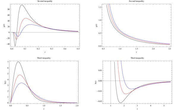
Figure 3: Here are represented the functions $g(r)$ and $h(r)$ for the IV case. The first picture shows the region that is inside the event horizon, where the function $g(r)$ is negative, that is, where the WEC is violated. Additionally, in a region that is outside the event horizon and that reaches infinity, $h(r)$ is negative. In all pictures $M=1$, and $q=0.55M$ (black), $q=0.65M$ (red) and $q=0.75M$ (blue).

4 Dynamical stability

We can examine the dynamical stability of these regular black hole solutions with respect to arbitrary linear fluctuations of the metric and electromagnetic field. For this we consider the following conditions that must be satisfied by the Hamiltonian $\mathcal{H}=\mathcal{H}(x)$ for all $0<x<x_{h}$ [36]

$$\mathcal{H} < 0\ ,$$ (30)

$$\mathcal{H}_{x} < 0\ ,$$ (31)

$$\mathcal{H}_{xx} < 0\ ,$$ (32)

$$3\mathcal{H}_{x} \leq xf(x)\mathcal{H}_{xx}\ ,$$ (33)

here the subscript $x$ denotes differentiation with respect to the new variable $x=q^{2}/r^{2}$ and we have defined the following value $x_{h}=q^{2}/r_{h}^{2}$.

Writing the Hamiltonian of each nonlinear electrodynamics model in terms of the variable $x$ we directly verify that inequalities (30-33) hold. In Table 1 these Hamiltonians are listed in terms of the invariant $\mathcal{P}$ and in terms of the variable $x$, where

$$\mathcal{P}=\frac{1}{4}P_{\mu\nu}P^{\mu\nu}=-\frac{q^{2}}{2r^{4}}\,.$$ (34)

And the following notation is used for abbreviation

$$s=\frac{|q|}{2M}\,\,\,\,\,\,\,\,,\,\,\,\,\,\,\,\,w=\left(\frac{|q|^{3/2}}{2^{3/4}M}\right)^{3}\,\,\,\,\,\,\,\,\mbox{and}\,\,\,\,\,\,\,\,U=\sqrt{-2q^{2}\mathcal{P}}\,.$$ (35)

Case	$\mathcal{H}(\mathcal{P})$	$\mathcal{H}(x)$	Reference
I	$\frac{\mathcal{P}}{\left(1+w\,(-\mathcal{P})^{3/4}\right)^{4/3}}$	$\frac{-x^{2}}{2q^{2}\left(1+w\left(\frac{1}{2q^{2}}x^{2}\right)^{3/4}\right)^{4/3}}$	[18]
II	$\frac{\mathcal{P}(1-3\,\sqrt{-2q^{2}\mathcal{P}})}{1+2\,\sqrt{-2q^{2}\mathcal{P}}}-\frac{3}{2sq^{2}}\left(\frac{\sqrt{-2q^{2}\mathcal{P}}}{1+\sqrt{-2q^{2}\mathcal{P}}}\right)^{5/2}$	$-\frac{x^{2}}{2q^{2}}\frac{(1-3x)}{(1+x)}-\frac{3}{2sq^{2}}\left(\frac{x}{1+x}\right)^{5/2}$	[19]
III	$\mathcal{P}e^{-sU}$	$-\frac{x^{2}}{2q^{2}}e^{-sx^{1/2}}$	[23]
IV	$\mathcal{P}\left[e^{-sU}+\frac{2U-4U^{3}}{\left(U^{2}+1\right)^{4}}\right]$	$-\frac{x^{2}}{2q^{2}}\left(e^{-sx^{1/2}}+\frac{2x^{1/2}-4x^{3/2}}{(x+1)^{4}}\right)$	novel

Table 1: Hamiltonians for each source of nonlinear electrodynamics considered in this paper as functions of $\mathcal{P}$ and $x$ respectively.

5 Quasinormal spectra

This section is devoted to introduce essential ingredients to study scalar perturbations in regular charged black hole background. Thus, we will review the basic theory of QNMs and the numerical method to compute the corresponding frequencies.

5.1 Wave equation for scalar perturbations

Let us assume the propagation of a test real scalar field, $\Phi$, in a four dimensional gravitational background. Being $S[g_{\mu\nu},\Phi]$ the corresponding action, we can write the following expression

$$S[g_{\mu\nu},\Phi]\equiv\frac{1}{2}\int\mathrm{d}^{4}x\sqrt{-g}\Bigg{[}\partial^{\mu}\Phi\partial_{\mu}\Phi+\xi R\Phi^{2}+\frac{1}{2}m^{2}\Phi^{2}\Bigg{]}\,.$$ (36)

In what follow, we will consider an auxiliary massless and neutral scalar field minimally coupled to gravity (i.e., we will set $\xi=0$ and $m=0$). Now, taking advantage of the Klein-Gordon equation (see [37, 38, 39, 40, 41, 42, 43] and references therein)

$$\frac{1}{\sqrt{-g}}\partial_{\mu}\left(\sqrt{-g}g^{\mu\nu}\partial_{\nu}\Phi\right)=0.$$ (37)

In this simplified scenario, the corresponding Klein-Gordon equation may be solved following the method of separation of variables in the appropriate coordinate system. Thus, taking into consideration the symmetries of the metric tensor, we will take an ansatz for the wave function in spherical coordinates $r,\theta,\phi$ as follows

$$\Phi(t,r,\theta,\phi)=e^{-i\omega t}\frac{\psi(r)}{r}Y_{\ell m}(\theta,\phi),$$ (38)

where the functions $Y_{\ell m}(\theta,\phi)$ are the conventional spherical harmonics which depend on the angular coordinates only [44], and $\omega$ is the unknown frequency to be determined after impose the concrete boundary conditions. Doing so, the relevant equation is then writen as

$$\begin{split}&\frac{\omega^{2}r^{2}}{f(r)}+\frac{r}{\psi(r)}\frac{d}{dr}\left[r^{2}f(r)\frac{d}{dr}\left(\frac{\psi(r)}{r}\right)\right]-\ell(\ell+1)=0.\end{split}$$ (39)

In the latter equation we have used the angular part, i.e.,

$$\begin{split}&\frac{1}{\sin\theta}\frac{\partial}{\partial\theta}\left(\sin\theta\frac{\partial Y(\Omega)}{\partial\theta}\right)+\frac{1}{\sin^{2}\theta}\frac{\partial^{2}Y(\Omega)}{\partial\phi^{2}}=-\ell(\ell+1)Y(\Omega),\end{split}$$ (40)

with $\ell(\ell+1)$ being the corresponding eigenvalue, and $\ell$ is the angular degree. The Klein-Gordon equation (Eq. (39)) can be rewriten in term of the tortoise coordinate $r_{*}$ in the Schrödinger-like form:

$$\frac{\mathrm{d}^{2}\psi(r)}{\mathrm{d}r_{*}^{2}}+\left[\omega^{2}-V(r)\right]\psi(r)=0\ ,$$ (41)

being the standard tortoise coordinate obtained using the following relation

$$r_{*}\equiv\int\frac{\mathrm{d}r}{f(r)}\ ,$$ (42)

while the effective potential barrier, $V(r)$, is computed to be

$$V(r)=f(r)\Bigg{[}\frac{\ell(\ell+1)}{r^{2}}+\frac{f^{\prime}(r)}{r}\Bigg{]}\ .$$ (43)

and the prime denotes a derivative with respect to $r$. To complete this part, we should specify the boundary conditions. Finally, the wave equation must be supplemented by the following boundary conditions

$$\Phi\rightarrow\>\exp(i\omega r_{*}),\;\;\;\;\;\;r_{*}\rightarrow-\infty\ ,$$ (44)

$$\Phi\rightarrow\>\exp(-i\omega r_{*}),\;\;\;\;\;\;r_{*}\rightarrow\infty\ .$$ (45)

Thus, as can be observed from the time dependence of the scalar wave function, $\Phi\sim\exp(-i\omega t)$, a frequency with a negative imaginary part means a decaying (stable) mode, whereas a frequency with a positive imaginary part means an increasing (unstable) mode.

In Fig. (4), we show the effective potential for the four models discussed above. Thus, top-left panel corresponds to the first model, top-right panel corresponds to the second model, bottom-left panel corresponds to the third model and bottom-right panel corresponds to the fourth model. Also, The qualitative behavior of the effective potential for all cases is basically the same for the numerical values used. We have fixed the electric charge $q$ and the mass $M$ when the angular degree $\ell$ varies. Thus, we notice that when we increase the angular number, $\ell$, the effective potential increases too. Similarly, when $\ell$ increases, $r_{\text{max}}$ is modified and slightly shifted to the right (in all cases).

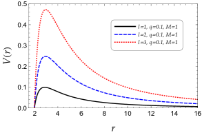
Figure 4: Effective potential for scalar perturbations against the radial coordinate for $q=0.1$, $M=1$ and $\ell=\{1,2,3\}$. Top-left panel corresponds to the first model, top-right panel corresponds to the second model, bottom-left panel corresponds to the third model and bottom-right panel corresponds to the fourth model.

5.2 Numerical computation via WKB method

Quasinormal modes are usually computed i) analytically (when it is possible), and ii) numerically. In particular, analytical computations are possible for instance: i) when the effective potential barrier takes the form of the well-known Pöschl-Teller potential [45, 46, 47, 48, 49, 50], or ii) when the differential equation (for the radial part of the wave function) can be recast into the Gauss’ hypergeometric function [51, 52, 53, 54, 55, 56, 57].

It is very well-known that, in general, an exact analytic solution is not possible to achieve. The reason of that is the complexity and non-trivial structure of the differential equation involved. By the above reasons, it is usually necessary to employ one of the numerical approaches available in the literature. There are a large number of methods used to obtain, in an accuracy, the QN spectra of black holes. We can mention, for example: i) the Frobenius method [58, 59], ii) the generalization of the Frobenius series, iii) fit and interpolation approach, iv) the method of continued fraction [60, 61, 62], v) the asymptotic iteration method [63, 64, 65] although more methods are known to exist. For more details the interested reader may consult for instance [66].

Thus, although there are many numerical methods to obtain the QNMs, we shall focus here on one of the most popular up to now, i.e., the WKB semi-classical method (commonly implemented in elementary 1D quantum mechanical problems). The formalism and the details have been investigated extensively by many authors, increasing the order of the approximation. In light of the WKB semi-classical approximation is well-known [67, 68, 69, 70, 71], we will circumvent the inclusion of details. Following the WKB method, the QN spectra may be computed via the following expression

$$\omega_{n}^{2}=V_{0}+(-2V_{0}^{\prime\prime})^{1/2}\Lambda(n)-i\nu(-2V_{0}^{\prime\prime})^{1/2}[1+\Omega(n)]\,,$$ (46)

where i) $V_{0}^{\prime\prime}$ represent the second derivative of the potential (at the maximum), ii) $\nu=n+1/2$, $V_{0}$ is the maximum of the effective potential barrier, iii) $n=0,1,2...$ symbolizes the overtone number, while the functions $\Lambda(n),\Omega(n)$ are quite long and intricate expressions of $\nu$ (and derivatives of the potential at the maximum). The concrete form of above symbols can be found in [70].

Notice that the 3rd order approximation was first constructed by Iyer and Will in [68], and after that extended to higher orders. Thus, to perform our computations, we have used here a Wolfram Mathematica [72] notebook utilizing the WKB method at any order from one to six [73].

In the present work we have implemented the WKB method at sixth order. Besides, it should be mentioned that for a given angular degree, $\ell$, we have considered values $n<\ell$ only, since it is known that the method works well for high angular degrees. Higher order in the WKB approximation have been investigated in [74, 75, 76] where a recipe for simple, quick, efficient and accurate computations was provided. Moreover, notice that as the WKB series converges only asymptotically, there is no mathematically strict criterion for evaluation of an error according to [75]. However, the sixth/seventh order usually produces the best results. In a future study we shall perform an error analysis and employ the Padé approximants with the hope to achieve a higher accuracy.

Our main results, to be discussed below, are summarized in figures (5)-(11) and tables (2)-(5). The QNMs for scalar perturbations of the model III was studied in [77], although in that work energy conditions were not discussed. In the present work, we show the spectra for all 4 models for comparison reasons. Finally, for recent studies of QNMs in alternative backgrounds see [78, 79, 80, 81, 82, 83, 84, 85, 86] and references therein.

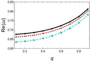
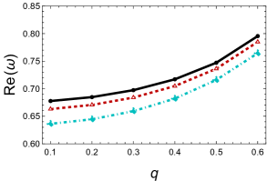
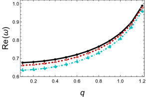
Figure 5: QNMs for all cases investigated with $M=1$, $\ell=3$ and $n=\{0,1,2\}$. Real part of $\omega$ against the electric charge $q$ for case I to IV from top left to bottom right. The color code is: i) solid black line for $n=0$, ii) dashed red line for $n=1$ and iii) dot-dashed cyan line for $n=2$.

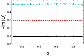
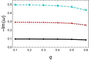
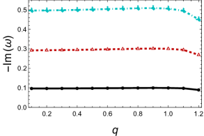
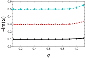
Figure 6: QNMs for all cases investigated with $M=1$, $\ell=3$ and $n=\{0,1,2\}$. Imaginary part of $\omega$ against the electric charge $q$ for case I to IV from top left to bottom right. The color code is: i) solid black line for $n=0$, ii) dashed red line for $n=1$ and iii) dot-dashed cyan line for $n=2$.

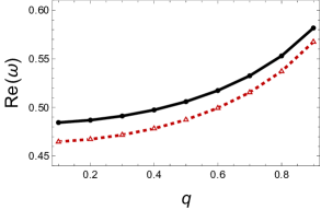
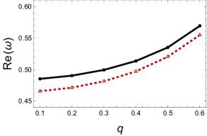
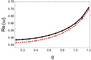
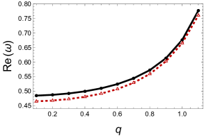
Figure 7: QNMs for all cases investigated with $M=1$, $\ell=2$ and $n=\{0,1\}$. Real part of $\omega$ against the electric charge $q$ for case I to IV from top left to bottom right. The color code is: i) solid black line for $n=0$ and ii) dashed red line for $n=1$.

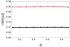
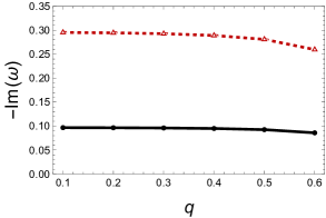
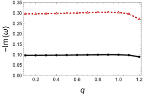
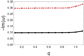
Figure 8: QNMs for all cases investigated with $M=1$, $\ell=2$ and $n=\{0,1\}$. Imaginary part of $\omega$ against the electric charge $q$ for case I to IV from top left to bottom right. The color code is: i) solid black line for $n=0$ and ii) dashed red line for $n=1$.

Figure 9: QNMs for all cases investigated with $M=1$, $\ell=1$ and $n=0$. Real part of $\omega$ against the electric charge $q$ for case I to IV from top left to bottom right.

Figure 10: QNMs for all cases investigated with $M=1$, $\ell=1$ and $n=0$. Imaginary part of $\omega$ against the electric charge $q$ for case I to IV from top left to bottom right.

Table 2: Quasinormal frequencies (varying $\ell$, $n$ and $q$) with $M=1$ for the first model considered in this work.

$q$	$n$	$\ell=1$	$\ell=2$	$\ell=3$
	0	0.293407 - 0.0978114 i	0.484455 - 0.0968185 i	0.676499 - 0.0965534 i
0.1	1		0.464698 - 0.2957730 i	0.661832 - 0.2924410 i
	2			0.634804 - 0.4962460 i
	0	0.294919 - 0.0979588 i	0.486929 - 0.0969738 i	0.679946 - 0.0967102 i
0.2	1		0.467290 - 0.2962050 i	0.665366 - 0.2928930 i
	2			0.638500 - 0.4969420 i
	0	0.297517 - 0.0981972 i	0.491179 - 0.0972258 i	0.685866 - 0.0969647 i
0.3	1		0.471746 - 0.2969000 i	0.671440 - 0.2936260 i
	2			0.644858 - 0.4980600 i
	0	0.301325 - 0.0985124 i	0.497411 - 0.0975606 i	0.694549 - 0.0973033 i
0.4	1		0.478295 - 0.2978110 i	0.680357 - 0.2945940 i
	2			0.654209 - 0.4995150 i
	0	0.306550 - 0.098875 i	0.505966 - 0.0979498 i	0.706468 - 0.0976983 i
0.5	1		0.487305 - 0.2988430 i	0.692614 - 0.2957090 i
	2			0.667090 - 0.5011440 i
	0	0.313519 - 0.0992245 i	0.517383 - 0.098335 i	0.722378 - 0.098092 i
0.6	1		0.499367 - 0.299802 i	0.709003 - 0.296789 i
	2			0.684359 - 0.502612 i
	0	0.322760 - 0.099430 i	0.532545 - 0.0985892 i	0.743515 - 0.0983592 i
0.7	1		0.515433 - 0.3002770 i	0.730816 - 0.2974410 i
	2			0.707399 - 0.5032100 i
	0	0.335193 - 0.0991747 i	0.55299 - 0.0984097 i	0.772039 - 0.0982003 i
0.8	1		0.537143 - 0.299286 i	0.760287 - 0.296729 i
	2			0.738566 - 0.501265 i
	0	0.352528 - 0.0975726 i	0.581718 - 0.0969387 i	0.812206 - 0.0967641 i
0.9	1		0.567456 - 0.294097 i	0.801669 - 0.292015 i
	2			0.781991 - 0.492131 i

Table 3: Quasinormal frequencies (varying $\ell$, $n$ and $q$) with $M=1$ for the second model considered in this work.

$q$	$n$	$\ell=1$	$\ell=2$	$\ell=3$
	0	0.293931 - 0.0976968 i	0.485289 - 0.0967053 i	0.677650 - 0.0964418 i
0.1	1		0.465678 - 0.2953930 i	0.663092 - 0.2920850 i
	2			0.636265 - 0.4955830 i
	0	0.297089 - 0.0974668 i	0.490386 - 0.0964901 i	0.684725 - 0.096233 i
0.2	1		0.471346 - 0.2945840 i	0.670586 - 0.291373 i
	2			0.644536 - 0.494117 i
	0	0.302702 - 0.0969435 i	0.499465 - 0.0960008 i	0.697331 - 0.0957558 i
0.3	1		0.481419 - 0.2928130 i	0.683930 - 0.2897840 i
	2			0.659232 - 0.4909520 i
	0	0.311423 - 0.095815 i	0.513636 - 0.0949421 i	0.717035 - 0.0947178 i
0.4	1		0.497062 - 0.2891280 i	0.704735 - 0.2864040 i
	2			0.682021 - 0.4844610 i
	0	0.324537 - 0.0932644 i	0.535188 - 0.0925256 i	0.747094 - 0.0923352 i
0.5	1		0.520478 - 0.2810110 i	0.736221 - 0.2788030 i
	2			0.715954 - 0.4703420 i
	0	0.344567 - 0.0864543 i	0.569504 - 0.0858761 i	0.795453 - 0.0857209 i
0.6	1		0.554955 - 0.2596170 i	0.784936 - 0.2581850 i
	2			0.764387 - 0.4336200 i

Table 4: Quasinormal frequencies (varying $\ell$, $n$ and $q$) with $M=1$ for the third model considered in this work.

$q$	$n$	$\ell=1$	$\ell=2$	$\ell=3$
	0	0.293406 - 0.0978115 i	0.484454 - 0.0968186 i	0.676498 - 0.0965535 i
0.1	1		0.464697 - 0.2957730 i	0.661831 - 0.2924410 i
	2			0.634803 - 0.4962470 i
	0	0.294912 - 0.0979604 i	0.486918 - 0.0969754 i	0.679930 - 0.0967117 i
0.2	1		0.467276 - 0.2962100 i	0.665349 - 0.2928980 i
	2			0.638480 - 0.4969520 i
	0	0.297479 - 0.0982059 i	0.491119 - 0.0972344 i	0.685783 - 0.0969731 i
0.3	1		0.471676 - 0.2969280 i	0.671349 - 0.2936530 i
	2			0.644753 - 0.4981100 i
	0	0.301197 - 0.098543 i	0.497208 - 0.0975909 i	0.694268 - 0.0973332 i
0.4	1		0.478056 - 0.2979120 i	0.680049 - 0.2946890 i
	2			0.653853 - 0.4996910 i
	0	0.306211 - 0.0989618 i	0.505422 - 0.0980355 i	0.705716 - 0.0977828 i
0.5	1		0.486670 - 0.2991280 i	0.691794 - 0.2959770 i
	2			0.666146 - 0.5016380 i
	0	0.312731 - 0.0994435 i	0.516118 - 0.0985504 i	0.720626 - 0.0983045 i
0.6	1		0.497895 - 0.3005140 i	0.707097 - 0.2974610 i
	2			0.682173 - 0.5038440 i
	0	0.321075 - 0.0999512 i	0.529823 - 0.0991003 i	0.739737 - 0.0988635 i
0.7	1		0.512292 - 0.3019550 i	0.726725 - 0.2990300 i
	2			0.702747 - 0.5061070 i
	0	0.331724 - 0.100411 i	0.547347 - 0.099614 i	0.764186 - 0.0993894 i
0.8	1		0.530719 - 0.303217 i	0.751847 - 0.3004640 i
	2			0.729098 - 0.5080280 i
	0	0.345441 - 0.100667 i	0.569988 - 0.099938 i	0.795797 - 0.0997299 i
0.9	1		0.554535 - 0.303809 i	0.784339 - 0.3012870 i
	2			0.763183 - 0.5087640 i
	0	0.363533 - 0.100345 i	0.599997 - 0.099705 i	0.837749 - 0.0995193 i
1.0	1		0.586058 - 0.302566 i	0.827435 - 0.3003710 i
	2			0.808316 - 0.5063320 i
	0	0.388499 - 0.0983738 i	0.641838 - 0.0978466 i	0.896398 - 0.0976899 i
1.1	1		0.629621 - 0.2961440 i	0.887419 - 0.2944380 i
	2			0.870552 - 0.4950440 i
	0	0.425303 - 0.0903157 i	0.706747 - 0.0895937 i	0.988322 - 0.0894092 i
1.2	1		0.692614 - 0.2704350 i	0.978313 - 0.2690350 i
	2			0.958506 - 0.4510810 i

Table 5: Quasinormal frequencies (varying $\ell$, $n$ and $q$) with $M=1$ for the fourth model considered in this work.

$q$	$n$	$\ell=1$	$\ell=2$	$\ell=3$
	0	0.293424 - 0.0978077 i	0.484482 - 0.0968149 i	0.676536 - 0.0965499 i
0.1	1		0.464729 - 0.2957610 i	0.661872 - 0.2924290 i
	2			0.634851 - 0.4962250 i
	0	0.295054 - 0.0979306 i	0.487144 - 0.0969461 i	0.680242 - 0.0966827 i
0.2	1		0.467541 - 0.2961110 i	0.665689 - 0.2928060 i
	2			0.638875 - 0.4967790 i
	0	0.297972 - 0.0981052 i	0.491906 - 0.0971357 i	0.686872 - 0.0968754 i
0.3	1		0.472599 - 0.2965980 i	0.672538 - 0.2933410 i
	2			0.646128 - 0.4975310 i
	0	0.302427 - 0.0983017 i	0.499174 - 0.0973574 i	0.696988 - 0.0971015 i
0.4	1		0.480351 - 0.2971310 i	0.683013 - 0.2939520 i
	2			0.657273 - 0.4983250 i
	0	0.308789 - 0.0984803 i	0.509549 - 0.0975801 i	0.711427 - 0.0973296 i
0.5	1		0.491464 - 0.2976050 i	0.698001 - 0.2945390 i
	2			0.673285 - 0.4989810 i
	0	0.317636 - 0.0985835 i	0.523963 - 0.0977681 i	0.731492 - 0.0975242 i
0.6	1		0.506959 - 0.2979010 i	0.718870 - 0.2949910 i
	2			0.695657 - 0.4993020 i
	0	0.329935 - 0.0985228 i	0.543939 - 0.0978954 i	0.759306 - 0.0976612 i
0.7	1		0.528496 - 0.2979180 i	0.747840 - 0.2952340 i
	2			0.726803 - 0.4991580 i
	0	0.347447 - 0.0981599 i	0.572111 - 0.0980226 i	0.798550 - 0.0978110 i
0.8	1		0.558897 - 0.2977960 i	0.788711 - 0.2954830 i
	2			0.770751 - 0.4989200 i
	0	0.373304 - 0.0976706 i	0.613285 - 0.0986527 i	0.856032 - 0.0985011 i
0.9	1		0.602778 - 0.2991690 i	0.848146 - 0.2973280 i
	2			0.833914 - 0.5013860 i
	0	0.404708 - 0.1053030 i	0.676058 - 0.1020630 i	0.944645 - 0.1018570 i
1.0	1		0.665054 - 0.3110080 i	0.936953 - 0.3070170 i
	2			0.923853 - 0.5169260 i
	0	0.46919 - 0.1120120 i	0.777111 - 0.1107050 i	1.088030 - 0.1111060 i
1.1	1		0.760849 - 0.3281150 i	1.074010 - 0.3323430 i
	2			1.046230 - 0.5477710 i

5.3 QNMs in the eikonal limit

In the eikonal regime (i.e., $\ell\gg 1$) the WKB approximation becomes increasingly accurate. Thus, we can obtain analytical expressions for the quasinormal frequencies. In such a limit ($\ell\rightarrow\infty$), the angular momentum term that dominates in the expression for the effective potential

$$V(r)\approx\frac{f(r)l^{2}}{r^{2}}\equiv l^{2}\sigma(r),$$ (47)

where for simplicity we have defined a new function $\sigma(r)\equiv f(r)/r^{2}$. It is possible to obtain the maximum of the potential, $r_{1}$ by solving the following algebraic equation

$$2f(r_{1})-r_{1}f^{\prime}(r)|_{r_{1}}=0.$$ (48)

The idea and formalism was treated in [87]. The QNMs, in the eikonal regime, are found to be

$$\omega(\ell\gg 1)=\Omega_{c}\ell-i\left(n+\frac{1}{2}\right)|\lambda_{L}|,$$ (49)

where the Lyapunov exponent $\lambda_{L}$ is given by [87]

$$\lambda_{L}=r_{1}^{2}\sqrt{\frac{\sigma^{\prime\prime}(r_{1})\sigma(r_{1})}{2}},$$ (50)

while the angular velocity $\Omega_{c}$ at the unstable null geodesic is given by [87]

$$\Omega_{c}=\frac{\sqrt{f(r_{1})}}{r_{1}}.$$ (51)

By applying the WKB approximation of 1st order, we can recover the same expression mentioned above for $\{\Omega_{c},\lambda_{L}\}$, see for instance [88]. Thus, although in the presence of non-linear electromagnetic sources photons follow the null trajectories of particular effective geometry rather than the null geodesics of the true geometry [89, 90, 91], the previous formulas for $\Omega_{c}$ and for $\lambda_{L}$ are the same. In particular, we know that i) the angular velocity determines the real part of the modes (where only the degree of angular momentum $\ell$ enters), and ii) the Lyapunov exponent determines the imaginary part of the modes (where only the overtone number $n$ appears). Thus, an analytic expression for the spectrum is found where

$$\omega_{R}(\ell\gg 1) \equiv \mbox{Re}(\omega)=\Omega_{c}\ell,$$ (52)

$$\omega_{I}(\ell\gg 1) \equiv \mbox{Im}(\omega)=-\left(n+\frac{1}{2}\right)|\lambda_{L}|,$$ (53)

In fig. (11) we present the angular velocity (left panel) and the absolute value of the Lyapunov exponent (right panel) versus $q$ assuming $M=1$ for all four models.

As far as the real part of the frequencies is concerned, the angular velocity, $\Omega_{c}$, increases monotonically with the electric charge in all cases. Regarding the imaginary part of the spectra, the Lyapunov exponent (its absolute value) exhibits a different behaviour from one model to another. In particular, in the cases of the models I and III, it reaches a maximum value first and subsequently it decreases (as opposed to the Bardeen black hole studied in [92], where it was found that $|\lambda_{L}|$ decreases monotonically with $q$). This is precisely the behaviour observed in the case of the standard RN geometry. In the case of model II, however, $|\lambda_{L}|$ monotonically decreases with $q$, similarly to [92]. Finally, model IV is the only case where the Lyapunov exponent increases rapidly with the electric charge as $q$ approaches extremality. The behaviour observed in the eikonal limit, $\ell\rightarrow\infty$, where the spectra were computed analytically, agrees with the behaviour seen in figures (5)-(10), where the frequencies were computed numerically for low angular degree, $\ell=1,2,3$. Therefore, we conclude that according to our findings, energy conditions imply a different pattern of the QN spectra.

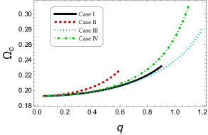
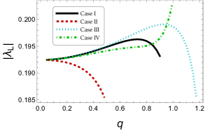
Figure 11: QNMs in the eikonal limit: Left panel: Angular velocity vs the electric charge for $M=1$. Right panel: Lyapunov exponent againt the electric charge for $M=1$. Both panels represent all the models, from case I to IV.

6 Conclusions

To summarize our work, we have discussed here regular charged BH solutions within GR coupled to non-linear Electrodynamics. In particular, we have studied four models exhibiting distinct behaviors depending on the associated energy conditions. The scalar invariants related to the curvature of space-time as well as the electric field are finite at the origin, while the solutions are characterized by the mass, $M$, and the electric charge, $q$. The QNMs of scalar perturbations have been computed for all four models considered in this work, both numerically adopting the WKB approximation and analytically in the eikonal limit, $\ell\rightarrow\infty$. All modes are characterized by a negative imaginary part. The impact of the electric charge, the angular degree, $\ell$, and the overtone number, $n$, has been investigated in detail. The effective potential barrier has been shown graphically as a function of the radial coordinate, $r$, for all non-linear models for fixed $\{M,q\}$ and varying the angular degree. As far as the eikonal limit is concerned, both the critical frequency (real part of the frequencies) and the Lyapunov exponent (imaginary part of the frequencies) have been shown graphically as a function of the electric charge assuming that $M=1$ for all four models studied here. The critical frequency was found to be a monotonically increasing function of $q$, while the Lyapunov exponent was observed to exhibit a behavior that depends on the energy conditions associated to the model at hand. Besides, the numerical values of the frequencies that were numerically computed have been displayed in tables (2)-(5), while for better visualization the real part as well as the imaginary part have been shown graphically as a function of the electric charge assuming $M=1$ for different values of the angular degree and the overtone number.

In this article, we investigated regular black holes assuming non-linear electrodynamics in four-dimensional space-time. Also, we reviewed the importance of the energy conditions in various solutions. In addition, we have obtained the scalar quasinormal frequencies in all four cases, using i) the WKB semi-analytic approach and ii) in the eikonal limit ($\ell\gg 1$). Our results reveal that all modes are characterized by a negative imaginary part under massless and neutral perturbations. The real and imaginary part versus the electric charge exhibit different behaviour from one model to another depending on the energy conditions. In other words we find a correlation between energy conditions and pattern in the QN spectra.

References

- [1] T. Regge and J. A. Wheeler, “Stability of a Schwarzschild singularity,” Phys. Rev. 108, 1063-1069 (1957).
- [2] F. J. Zerilli, “Effective potential for even parity Regge-Wheeler gravitational perturbation equations,” Phys. Rev. Lett. 24, 737-738 (1970).
- [3] F. J. Zerilli, “Gravitational field of a particle falling in a schwarzschild geometry analyzed in tensor harmonics,” Phys. Rev. D 2, 2141-2160 (1970).
- [4] F. J. Zerilli, “Perturbation analysis for gravitational and electromagnetic radiation in a reissner-nordstroem geometry,” Phys. Rev. D 9, 860-868 (1974).
- [5] V. Moncrief, “Gauge-invariant perturbations of Reissner-Nordstrom black holes,” Phys. Rev. D 12, 1526-1537 (1975).
- [6] S. A. Teukolsky, “Rotating black holes - separable wave equations for gravitational and electromagnetic perturbations,” Phys. Rev. Lett. 29, 1114-1118 (1972).
- [7] S. Chandrasekhar, “The mathematical theory of black holes,” OXFORD, UK: CLARENDON (1985) 646 P.
- [8] I. Dymnikova, “Vacuum nonsingular black hole,” Gen. Rel. Grav. 24, 235-242 (1992).
- [9] P. Nicolini, A. Smailagic and E. Spallucci, “Noncommutative geometry inspired Schwarzschild black hole,” Phys. Lett. B 632, 547-551 (2006).
- [10] S. A. Hayward, “Formation and evaporation of regular black holes,” Phys. Rev. Lett. 96, 031103 (2006).
- [11] L. Xiang, Y. Ling and Y. G. Shen, “Singularities and the Finale of Black Hole Evaporation,” Int. J. Mod. Phys. D 22, 1342016 (2013).
- [12] S. G. Ghosh, “A nonsingular rotating black hole,” Eur. Phys. J. C 75, no.11, 532 (2015).
- [13] V. P. Frolov, “Notes on nonsingular models of black holes,” Phys. Rev. D 94, no.10, 104056 (2016).
- [14] V. P. Frolov and A. Zelnikov, “Quantum radiation from an evaporating nonsingular black hole,” Phys. Rev. D 95, no.12, 124028 (2017).
- [15] J. M. Bardeen “Non-singular general-relativistic gravitational collapse,” in Proceedings of GR5, Tbilisi, U.S.S.R, p.174 (1968).
- [16] E. Ayon-Beato and A. Garcia, “The Bardeen model as a nonlinear magnetic monopole,” Phys. Lett. B 493, 149-152 (2000).
- [17] M. E. Rodrigues and M. V. d. Silva, “Bardeen Regular Black Hole With an Electric Source,” JCAP 06, 025 (2018).
- [18] L. Balart and E. C. Vagenas, Regular black hole metrics and the weak energy condition, Phys. Lett. B 730, 14 (2014). [arXiv:1401.2136 [gr-qc]].
- [19] E. Ayon-Beato and A. Garcia, Regular black hole in general relativity coupled to nonlinear electrodynamics, Phys. Rev. Lett. 80, 5056 (1998). [gr-qc/9911046].
- [20] E. Ayon-Beato and A. Garcia, New regular black hole solution from nonlinear electrodynamics, Phys. Lett. B 464, 25 (1999). [hep-th/9911174].
- [21] K. A. Bronnikov, Regular magnetic black holes and monopoles from nonlinear electrodynamics, Phys. Rev. D 63, 044005 (2001). [gr-qc/0006014].
- [22] I. Dymnikova, “Regular electrically charged structures in nonlinear electrodynamics coupled to general relativity,” Class. Quant. Grav. 21, 4417-4429 (2004). [arXiv:gr-qc/0407072 [gr-qc]].
- [23] L. Balart and E. C. Vagenas, Regular black holes with a nonlinear electrodynamics source, Phys. Rev. D 90, no. 12, 124045 (2014). [arXiv:1408.0306 [gr-qc]].
- [24] W. Javed, S. Riaz and A. Övgün, “Weak Deflection Angle and Greybody Bound of Magnetized Regular Black Hole,” Universe 8 (2022) no.5, 262 [arXiv:2205.02229 [gr-qc]].
- [25] A. Övgün, “Weak field deflection angle by regular black holes with cosmic strings using the Gauss-Bonnet theorem,” Phys. Rev. D 99 (2019) no.10, 104075 [arXiv:1902.04411 [gr-qc]].
- [26] K. Jusufi, A. Övgün, J. Saavedra, Y. Vásquez and P. A. González, “Deflection of light by rotating regular black holes using the Gauss-Bonnet theorem,” Phys. Rev. D 97 (2018) no.12, 124024 [arXiv:1804.00643 [gr-qc]].
- [27] E. Contreras, Á. Rincón, B. Koch and P. Bargueño, “A regular scale-dependent black hole solution,” Int. J. Mod. Phys. D 27 (2017) no.03, 1850032 [arXiv:1711.08400 [gr-qc]].
- [28] G. Melgarejo, E. Contreras and P. Bargueño, “Regular black holes with exotic topologies,” Phys. Dark Univ. 30 (2020), 100709
- [29] E. Contreras, F. Tello-Ortiz and S. K. Maurya, “Regular decoupling sector and exterior solutions in the context of MGD,” Class. Quant. Grav. 37 (2020) no.15, 155002 [arXiv:2002.12444 [gr-qc]].
- [30] S. W. Hawking and G. F. R. Ellis, “The Large Scale Structure of Space-Time,” Cambridge University Press, 2011.
- [31] R. M. Wald, “General Relativity,” Chicago Univ. Pr., 1984.
- [32] V. P. Frolov and I. D. Novikov, “Black hole physics: Basic concepts and new developments,”
- [33] O. B. Zaslavskii, “Regular black holes and energy conditions,” Phys. Lett. B 688, 278-280 (2010). [arXiv:1004.2362 [gr-qc]].
- [34] I. Dymnikova, “Cosmological term as a source of mass,” Class. Quant. Grav. 19, 725-740 (2002). [arXiv:gr-qc/0112052 [gr-qc]].
- [35] M. E. Rodrigues, E. L. B. Junior and M. V. de Sousa Silva, “Using dominant and weak energy conditions for build new classe of regular black holes,” JCAP 02, 059 (2018). [arXiv:1705.05744 [physics.gen-ph]].
- [36] C. Moreno and O. Sarbach, “Stability properties of black holes in selfgravitating nonlinear electrodynamics,” Phys. Rev. D 67, 024028 (2003). [arXiv:gr-qc/0208090 [gr-qc]].
- [37] L. C. B. Crispino, A. Higuchi, E. S. Oliveira and J. V. Rocha, “Greybody factors for nonminimally coupled scalar fields in Schwarzschild–de Sitter spacetime,” Phys. Rev. D 87 (2013) 104034 [arXiv:1304.0467 [gr-qc]].
- [38] P. Kanti, T. Pappas and N. Pappas, “Greybody factors for scalar fields emitted by a higher-dimensional Schwarzschild–de Sitter black hole,” Phys. Rev. D 90 (2014) no.12, 124077 [arXiv:1409.8664 [hep-th]].
- [39] T. Pappas, P. Kanti and N. Pappas, “Hawking radiation spectra for scalar fields by a higher-dimensional Schwarzschild–de Sitter black hole,” Phys. Rev. D 94 (2016) no.2, 024035 [arXiv:1604.08617 [hep-th]].
- [40] G. Panotopoulos and Á. Rincón, “Quasinormal modes of five-dimensional black holes in non-commutative geometry,” Eur. Phys. J. Plus 135 (2020) no.1, 33 [arXiv:1910.08538 [gr-qc]].
- [41] Á. Rincón, P. A. Gonzalez, G. Panotopoulos, J. Saavedra and Y. Vasquez, “Quasinormal modes for a non-minimally coupled scalar field in a five-dimensional Einstein–Power–Maxwell background,” Eur. Phys. J. Plus 137 (2022) no.11, 1278 [arXiv:2112.04793 [gr-qc]].
- [42] P. A. González, E. Papantonopoulos, Á. Rincón and Y. Vásquez, “Quasinormal modes of massive scalar fields in four-dimensional wormholes: Anomalous decay rate,” Phys. Rev. D 106 (2022) no.2, 024050 [arXiv:2205.06079 [gr-qc]].
- [43] Á. Rincón and V. Santos, “Greybody factor and quasinormal modes of Regular Black Holes,” Eur. Phys. J. C 80 (2020) no.10, 910 [arXiv:2009.04386 [gr-qc]].
- [44] C. Muller, in Lecture Notes in Mathematics: Spherical Harmonics (Springer-Verlag, Berlin-Heidelberg, 1966).
- [45] G. Poschl and E. Teller, “Bemerkungen zur Quantenmechanik des anharmonischen Oszillators,” Z. Phys. 83 (1933) 143.
- [46] V. Ferrari and B. Mashhoon, “New approach to the quasinormal modes of a black hole,” Phys. Rev. D 30 (1984) 295.
- [47] V. Cardoso and J. P. S. Lemos, “Scalar, electromagnetic and Weyl perturbations of BTZ black holes: Quasinormal modes,” Phys. Rev. D 63 (2001) 124015 [gr-qc/0101052].
- [48] V. Cardoso and J. P. S. Lemos, “Quasinormal modes of the near extremal Schwarzschild-de Sitter black hole,” Phys. Rev. D 67 (2003) 084020 [gr-qc/0301078].
- [49] C. Molina, “Quasinormal modes of d-dimensional spherical black holes with near extreme cosmological constant,” Phys. Rev. D 68 (2003) 064007 [gr-qc/0304053].
- [50] G. Panotopoulos, “Electromagnetic quasinormal modes of the nearly-extremal higher-dimensional Schwarzschild–de Sitter black hole,” Mod. Phys. Lett. A 33 (2018) no.23, 1850130 [arXiv:1807.03278 [gr-qc]].
- [51] D. Birmingham, “Choptuik scaling and quasinormal modes in the AdS / CFT correspondence,” Phys. Rev. D 64 (2001) 064024 [hep-th/0101194].
- [52] S. Fernando, “Quasinormal modes of charged dilaton black holes in (2+1)-dimensions,” Gen. Rel. Grav. 36 (2004) 71 [hep-th/0306214].
- [53] S. Fernando, “Quasinormal modes of charged scalars around dilaton black holes in 2+1 dimensions: Exact frequencies,” Phys. Rev. D 77 (2008) 124005 [arXiv:0802.3321 [hep-th]].
- [54] P. Gonzalez, E. Papantonopoulos and J. Saavedra, “Chern-Simons black holes: scalar perturbations, mass and area spectrum and greybody factors,” JHEP 08 (2010), 050 [arXiv:1003.1381 [hep-th]].
- [55] K. Destounis, G. Panotopoulos and Á. Rincón, “Stability under scalar perturbations and quasinormal modes of 4D Einstein–Born–Infeld dilaton spacetime: exact spectrum,” Eur. Phys. J. C 78 (2018) no.2, 139 [arXiv:1801.08955 [gr-qc]].
- [56] A. Ovgün and K. Jusufi, “Quasinormal Modes and Greybody Factors of gravity minimally coupled to a cloud of strings in Dimensions,” Annals Phys. 395, 138 (2018) [arXiv:1801.02555 [gr-qc]].
- [57] Á. Rincón and G. Panotopoulos, “Greybody factors and quasinormal modes for a nonminimally coupled scalar field in a cloud of strings in (2+1)-dimensional background,” Eur. Phys. J. C 78, no. 10, 858 (2018) [arXiv:1810.08822 [gr-qc]].
- [58] G. T. Horowitz and V. E. Hubeny, Phys. Rev. D62, 024027 (2000), [hep-th/9909056].
- [59] A. O. Starinets, Phys. Rev. D66, 124013 (2002), [hep-th/0207133].
- [60] E. W. Leaver, Proc. Roy. Soc. Lond. A402, 285 (1985).
- [61] E. W. Leaver, J. Math. Phys. 27, 1238 (1986).
- [62] E. W. Leaver, Phys. Rev. D34, 384 (1986).
- [63] H. T. Cho, A. S. Cornell, J. Doukas, T. R. Huang and W. Naylor, “A New Approach to Black Hole Quasinormal Modes: A Review of the Asymptotic Iteration Method,” Adv. Math. Phys. 2012 (2012), 281705 [arXiv:1111.5024 [gr-qc]].
- [64] Ciftci, H., Hall, R. L., & Saad, N. 2003, Journal of Physics A Mathematical General, 36, 11807. doi:10.1088/0305-4470/36/47/008
- [65] H. Ciftci, R. L. Hall and N. Saad, “Perturbation theory in a framework of iteration methods,” Phys. Lett. A 340 (2005), 388-396 [arXiv:math-ph/0504056 [math-ph]].
- [66] R. A. Konoplya and A. Zhidenko, “Quasinormal modes of black holes: From astrophysics to string theory,” Rev. Mod. Phys. 83 (2011) 793 [arXiv:1102.4014 [gr-qc]].
- [67] B. F. Schutz and C. M. Will, “Black Hole Normal Modes: A Semianalytic Approach,” Astrophys. J. 291 (1985) L33.
- [68] S. Iyer and C. M. Will, “Black Hole Normal Modes: A WKB Approach. 1. Foundations and Application of a Higher Order WKB Analysis of Potential Barrier Scattering,” Phys. Rev. D 35 (1987) 3621.
- [69] S. Iyer, “Black Hole Normal Modes: A Wkb Approach. 2. Schwarzschild Black Holes,” Phys. Rev. D 35 (1987) 3632.
- [70] K. D. Kokkotas and B. F. Schutz, “Black Hole Normal Modes: A WKB Approach. 3. The Reissner-Nordstrom Black Hole,” Phys. Rev. D 37 (1988) 3378.
- [71] E. Seidel and S. Iyer, “Black Hole Normal Modes: A Wkb Approach. 4. Kerr Black Holes,” Phys. Rev. D 41 (1990) 374.
- [72] http://www.wolfram.com
- [73] R. A. Konoplya and A. Zhidenko, “Passage of radiation through wormholes of arbitrary shape,” Phys. Rev. D 81 (2010) 124036 [arXiv:1004.1284 [hep-th]].
- [74] J. Matyjasek and M. Opala, “Quasinormal modes of black holes. The improved semianalytic approach,” Phys. Rev. D 96 (2017) no.2, 024011 [arXiv:1704.00361 [gr-qc]].
- [75] R. A. Konoplya, A. Zhidenko and A. F. Zinhailo, “Higher order WKB formula for quasinormal modes and grey-body factors: recipes for quick and accurate calculations,” Class. Quant. Grav. 36 (2019) 155002 [arXiv:1904.10333 [gr-qc]].
- [76] Y. Hatsuda, “Quasinormal modes of black holes and Borel summation,” arXiv:1906.07232 [gr-qc].
- [77] G. Panotopoulos and Á. Rincón, “Quasinormal modes of regular black holes with non linear-Electrodynamical sources,” Eur. Phys. J. Plus 134, no.6, 300 (2019) [arXiv:1904.10847 [gr-qc]].
- [78] M. Okyay and A. Övgün, JCAP 01 (2022) no.01, 009 [arXiv:2108.07766 [gr-qc]].
- [79] A. Ovgün and K. Jusufi, “Quasinormal Modes and Greybody Factors of gravity minimally coupled to a cloud of strings in Dimensions,” Annals Phys. 395 (2018), 138-151 [arXiv:1801.02555 [gr-qc]].
- [80] R. C. Pantig, L. Mastrototaro, G. Lambiase and A. Övgün, “Shadow, lensing, quasinormal modes, greybody bounds and neutrino propagation by dyonic ModMax black holes,” Eur. Phys. J. C 82 (2022) no.12, 1155 [arXiv:2208.06664 [gr-qc]].
- [81] P. A. González, Á. Rincón, J. Saavedra and Y. Vásquez, “Superradiant instability and charged scalar quasinormal modes for (2+1)-dimensional Coulomb-like AdS black holes from nonlinear electrodynamics,” Phys. Rev. D 104 (2021) no.8, 084047 [arXiv:2107.08611 [gr-qc]].
- [82] G. Panotopoulos and Á. Rincón, “Quasinormal spectra of scale-dependent Schwarzschild–de Sitter black holes,” Phys. Dark Univ. 31 (2021), 100743 [arXiv:2011.02860 [gr-qc]].
- [83] Á. Rincón and G. Panotopoulos, “Quasinormal modes of an improved Schwarzschild black hole,” Phys. Dark Univ. 30 (2020), 100639 [arXiv:2006.11889 [gr-qc]].
- [84] Á. Rincón and G. Panotopoulos, “Quasinormal modes of scale dependent black holes in ( 1+2 )-dimensional Einstein-power-Maxwell theory,” Phys. Rev. D 97 (2018) no.2, 024027 [arXiv:1801.03248 [hep-th]].
- [85] G. Panotopoulos and Á. Rincón, “Quasinormal modes of black holes in Einstein-power-Maxwell theory,” Int. J. Mod. Phys. D 27 (2017) no.03, 1850034 [arXiv:1711.04146 [hep-th]].
- [86] R. Avalos and E. Contreras, “Quasi normal modes of hairy black holes at higher-order WKB approach,” Eur. Phys. J. C 83 (2023) no.2, 155 [arXiv:2302.09148 [gr-qc]].
- [87] V. Cardoso, A. S. Miranda, E. Berti, H. Witek and V. T. Zanchin, “Geodesic stability, Lyapunov exponents and quasinormal modes,” Phys. Rev. D 79 (2009) 064016 [arXiv:0812.1806 [hep-th]].
- [88] S. Ponglertsakul, P. Burikham and L. Tannukij, “Quasinormal modes of black strings in de Rham–Gabadadze–Tolley massive gravity,” Eur. Phys. J. C 78 (2018) no.7, 584 [arXiv:1803.09078 [gr-qc]].
- [89] N. Bretón and L. A. Lopez, “Quasinormal modes of nonlinear electromagnetic black holes from unstable null geodesics,” Phys. Rev. D 94 (2016) no.10, 104008 [arXiv:1607.02476 [gr-qc]].
- [90] N. Bretón, T. Clark and S. Fernando, “Quasinormal modes and absorption cross-sections of Born–Infeld–de Sitter black holes,” Int. J. Mod. Phys. D 26 (2017) no.10, 1750112 [arXiv:1703.10070 [gr-qc]].
- [91] E. Chaverra, J. C. Degollado, C. Moreno and O. Sarbach, “Black holes in nonlinear electrodynamics: Quasinormal spectra and parity splitting,” Phys. Rev. D 93 (2016) no.12, 123013 [arXiv:1605.04003 [gr-qc]].
- [92] S. Fernando and J. Correa, “Quasinormal Modes of Bardeen Black Hole: Scalar Perturbations,” Phys. Rev. D 86 (2012) 064039 [arXiv:1208.5442 [gr-qc]].