Bound-preserving discontinuous Galerkin methods for compressible two-phase flows in porous media

Abstract.

This paper presents a numerical study of immiscible, compressible two-phase flows in porous media, that takes into account heterogeneity, gravity, anisotropy and injection/production wells. We formulate a fully implicit stable discontinuous Galerkin solver for this system that is accurate, that respects maximum principle for the approximation of saturation, and that is locally mass conservative. To completely eliminate the overshoot and undershoot phenomena, we construct a flux limiter that produces bound-preserving elementwise average of the saturation. The addition of a slope limiter allows to recover a pointwise bound-preserving discrete saturation. Numerical results show that both maximum principle and monotonicity of the solution are satisfied. The proposed flux limiter does not impact the local mass error and the number of nonlinear solver iterations.

1. Introduction

Compressible multiphase flows in porous media occur in many applications such as subsurface carbon sequestration. Compressibility is modeled by the dependence of the fluid mass densities and rock porosity on the phase pressure. This work formulates a stable discontinuous Galerkin method for compressible two-phase flows in heterogeneous porous media; the main contribution being that the scheme satisfies a maximum principle for the numerical phase saturation.

The literature on numerical methods for two-phase flows in porous media is large, particularly for the case of incompressible phases [Chen et al., 2006; Hoteit and Firoozabadi, 2008; Bastian, 2014; Hou et al., 2016; Doyle et al., 2020]. It is known that suitable methods for porous media flows should satisfy a local mass conservation property. Both finite volume methods and discontinuous Galerkin methods are good candidates. There are other desirable properties such as maximum principle and monotonicity. On the one hand, finite volume methods produce piecewise constant approximation of the saturation that satisfies physical bounds [Michel, 2003; Droniou, 2014; Ghilani et al., 2019]. On the other hand, finite volume methods are numerically diffusive and require Voronoi-type grids for unstructured meshes, which can be challenging to construct for anisotropic heterogeneous media [Aavatsmark, 2002; de Carvalho et al., 2007; Contreras et al., 2021]. Discontinuous Galerkin (DG) methods overcome the shortcomings of finite volume methods because they belong to the class of variational problems like finite element methods. DG methods can be of arbitrary order, are adapted to any unstructured meshes, and in the case of convection-dominated problems, they produce sharp fronts with negligible numerical diffusion. However in the neighborhood of the saturation front, overshoot and undershoot phenomena may occur as the maximum principle for the DG solution is not guaranteed [Klieber and Riviere, 2006; Epshteyn and Riviere, 2007; Ern et al., 2010; Bastian, 2014; Jamei and Ghafouri, 2016]. These overshoot and undershoot phenomena remain bounded throughout the simulation and it is possible to reduce the amount of overshoot/undershoot by mesh refinement, or by projecting phase velocities into H(div) conforming spaces, by varying the penalty parameters, or by using slope limiters [Hoteit et al., 2004; Krivodonova, 2007; Kuzmin, 2010, 2013; Kuzmin and Gorb, 2012]. However, a complete elimination of the overshoot/undershoot has been challenging to achieve.

Recently in [Joshaghani et al., 2022], we proposed a DG method combined with a flux limiter for solving the immiscible incompressible two-phase flows in porous media. The DG saturations are shown to satisfy a maximum principle, in the sense that solutions do not exhibit any overshoot and undershoot phenomena. This current work is an extension of [Joshaghani et al., 2022] to the case of compressible phases. This is a more complicated problem because of the dependency of the coefficients (phase densities and porous medium porosity) with respect to the pressure. We have observed that the amount of overshoot and undershoot in DG solutions is larger for compressible flows than for incompressible flows. The numerical method is fully implicit and the nonlinear equations are solved by Newton’s method. The novel contribution is the construction of a new flux limiter that takes into account the dependence of the densities and porosity on the unknown. The proposed flux limiter is related to flux-corrected transport algorithms for the solution of conservation laws [Frank et al., 2019; Kuzmin and Gorb, 2012]. We show that the resulting method respects the maximum principle and is locally mass conservative for several problems taking into account gravity and heterogeneity. To our knowledge, this work is the first to present a DG-based scheme for compressible two-phase flows, that does not violate the maximum principle. An outline of the paper is as follows: after a brief introduction of the model equations in Section 2, the proposed numerical method is formulated in Section 3. Numerical results and conclusions follow.

2. Governing equations

The mathematical model describing the flow of a wetting phase (with saturation $s$ and pressure $p$) and a non-wetting phase in a domain $\Omega\subset\mathbb{R}^{2}$ over the time interval $[0,T]$ is:

$$\frac{\partial}{\partial t}\left(\phi(p)\rho_{\ell}(p)(1-s)\right)-\nabla\cdot\left(\rho_{\ell}(p)\lambda_{\ell}(s)K(\nabla p-\rho_{\ell}(p)\mathbf{g})\right)=\rho_{\ell}(p)q_{\ell},$$ (2.1)

$$\frac{\partial}{\partial t}\left(\phi(p)\rho_{w}(p)s\right)-\nabla\cdot\left(\rho_{w}(p)\lambda_{w}(s)K(\nabla p-\rho_{w}(p)\mathbf{g})\right)=\rho_{w}(p)q_{w}.$$ (2.2)

Since the capillary pressure is neglected, the mathematical model is a system of nonlinear hyperbolic equations. Compressibility of the phases and the medium is modeled by the following dependence of densities and porosity on the pressure:

$$\phi(p)=\phi^{0}(1+c_{r}p),\quad\rho_{\ell}(p)=\rho_{\ell}^{0}(1+c_{\ell}p),\quad\rho_{w}(p)=\rho_{w}^{0}(1+c_{w}p),$$

where the rock and fluid compressibilities, $c_{r},c_{\ell},c_{w}$ and the reference porosity and densities, $\phi_{0},\rho_{w}^{0},\rho_{\ell}^{0}$ are given constants. The absolute permeability, $K$, of the medium is either a positive scalar or a symmetric positive definite matrix $K$ that may vary in space. The phase mobilities are $\lambda_{\ell}$ and $\lambda_{w}$ for the non-wetting phase and wetting phase respectively; they are given functions of saturation and also depend on the phase viscosities $\mu_{\ell},\mu_{w}$. In this work, the commonly used Brooks-Corey model is considered:

$$\lambda_{w}(s_{e})=\frac{s_{e}^{2}}{\mu_{w}},\quad\lambda_{\ell}(s_{e})=\frac{(1-s_{e})^{2}}{\mu_{\ell}},$$ (2.3)

where effective saturation is defined as:

$$s_{e}=\frac{s-s_{rw}}{1-s_{rw}-s_{r\ell}}.$$ (2.4)

The residual saturation for wetting phase and non-wetting phase are denoted by $s_{rw}$ and $s_{r\ell}$ respectively. The functions $q_{\ell}$ and $q_{w}$ are given source/sink functions. The boundary is partitioned into $\partial\Omega=\Gamma^{\mathrm{D},p}\cup\Gamma^{\mathrm{N},p}=\Gamma^{\mathrm{D},s}\cup\Gamma^{\mathrm{out}}\cup\Gamma^{\mathrm{N},s}$. We prescribe Dirichlet and flux boundary conditions on $\Gamma^{\mathrm{D},p}\cup\Gamma^{\mathrm{D},s}$ and $\Gamma^{\mathrm{N},p}\cup\Gamma^{\mathrm{N},s}$ respectively, as follows:

$$p=g^{p} \quad\mathrm{on}\;\Gamma^{\mathrm{D},p},$$

$$s=g^{s} \quad\mathrm{on}\;\Gamma^{\mathrm{D},s},$$

$$\rho_{\ell}(p)\lambda_{\ell}(p)K(\nabla p-\rho_{\ell}(p)\mathbf{g})\cdot{\mathbf{n}}=j^{p} \quad\mathrm{on}\;\Gamma^{\mathrm{N},p},$$

$$\rho_{w}(p)\lambda_{w}(p)K(\nabla p-\rho_{w}(p)\mathbf{g})\cdot{\mathbf{n}}=j^{s} \quad\mathrm{on}\;\Gamma^{\mathrm{N},s}.$$

We will consider the case of flows driven by boundary conditions and the case of flows driven by wells (source/sink functions). For the latter, only homogeneous Neumann boundary conditions are imposed on the boundary. The source/sink functions depend on the saturation as follows

$$q_{\alpha}(s)=f_{\alpha}(s_{\mathrm{in}})\bar{q}-f_{\alpha}(s)\underline{q},\quad\alpha=w,\ell,$$ (2.5)

where $s_{\mathrm{in}}$ is the injected saturation value, $\bar{q}$ and $\underline{q}$ are the injection and production well flow rates respectively, and $f_{\alpha}$ is the fractional flow for phase $\alpha$. The fractional flows are related to the mobilities by:

$$f_{w}(s)=\frac{\lambda_{w}(s)}{\lambda_{w}(s)+\lambda_{\ell}(s)}\quad\mbox{and}\quad f_{\ell}(s)=1-f_{w}(s).$$ (2.6)

For the case of flows driven by boundary conditions, we assume that the Dirichlet boundary for the saturation is strictly included in the Dirichlet boundary for the pressure and the outflow boundary is the complement $\Gamma^{\mathrm{out}}=\Gamma^{p,\mathrm{D}}\setminus\Gamma^{s,\mathrm{D}}$. No boundary conditions are assumed for the saturation on the outflow boundary. The source/sink functions are set to zero.

Finally, the initial pressure and saturation are denoted by $p_{0}$ and $s_{0}$.

3. Numerical Method

We discretize (2.1)-(2.2) by a fully implicit interior penalty discontinuous Galerkin method. We first set some notation. The domain $\Omega$ is decomposed into a non-degenerate partition $\mathcal{E}_{h}=\{E\}_{E}$ consisting of $N_{h}$ triangular elements of maximum diameter $h$. Let $\Gamma_{h}$ denote the set of all edges and $\Gamma_{h}^{i}$ denote the set of interior edges. For any $e\in\Gamma_{h}^{i}$, fix a unit normal vector $\mathbf{n}_{e}$ and denote by $E^{+}$ and $E^{-}$ the elements that share the edge $e$ such that the vector $\mathbf{n}_{e}$ is directed from $E^{+}$ to $E^{-}$. We define the jump and average of a scalar function $\xi$ on $e$ as follows:

$$\llbracket\xi\rrbracket=\xi|_{E^{+}}-\xi|_{E^{-}},\quad\{\!\!\{\xi\}\!\!\}=\frac{1}{2}\left(\xi|_{E^{+}}+\xi|_{E^{-}}\right).$$ (3.1)

By convention, if $e$ belongs to the boundary $\partial\Omega$, then the jump and average of $\xi$ on $e$ coincide with the trace of $\xi$ on $e$ and the normal vector $\mathbf{n}_{e}$ coincides with the outward normal $\mathbf{n}$. Let $\mathbb{P}_{1}(E)$ be the space of linear polynomials on an element $E$. The discontinuous finite element space of order one is:

$$\mathcal{D}(\mathcal{E}_{h})=\left\{\xi\in L^{2}(\Omega):\xi|_{E}\in\mathbb{P}_{1}(E),\,\forall E\in\mathcal{E}_{h}\right\}.$$ (3.2)

The time interval $T$ is divided into $N_{\tau}$ equal subintervals of length $\tau$. Let $P_{n}$ and $S_{n}$ denote the numerical solutions at time $t_{n}$. The proposed discontinuous Galerkin scheme for equations (2.1)–(2.2) reads: Given $(P_{n},S_{n})\in\mathcal{D}(\mathcal{E}_{h})\times\mathcal{D}(\mathcal{E}_{h})$, find $(P_{n+1},S_{n+1})\in\mathcal{D}(\mathcal{E}_{h})\times\mathcal{D}(\mathcal{E}_{h})$ such that for all $\xi\in\mathcal{D}(\mathcal{E}_{h})$:

$$\frac{1}{\tau}\sum_{E\in\mathcal{E}_{h}}\int_{E}\phi(P_{n+1})\rho_{\ell}(P_{n+1})(1-S_{n+1})\xi+\sum_{E\in\mathcal{E}_{h}}\int_{E}\rho_{\ell}(P_{n+1})\lambda_{\ell}(S_{n+1})K\big{(}\nabla P_{n+1}-\rho_{\ell}(P_{n+1})\mathbf{g}\big{)}\cdot\nabla\xi$$

$$-\sum_{e\in\Gamma^{i}_{h}}\int_{e}(\lambda_{\ell}(S_{n+1}))^{\uparrow\mathbf{v}_{\ell}^{n}}\,\{\!\!\{\rho_{\ell}(P_{n})K\big{(}\nabla P_{n+1}-\rho_{\ell}(P_{n+1})\mathbf{g}\big{)}\cdot{\mathbf{n}_{e}}\}\!\!\}\llbracket\xi\rrbracket$$

$$-\sum_{e\in\Gamma^{\mathrm{D},p}}\int_{e}\lambda_{\ell}(S_{n+1})K{\rho_{\ell}(P_{n+1})\big{(}\nabla P_{n+1}-\rho_{\ell}(P_{n+1})\mathbf{g}\big{)}}\cdot{\mathbf{n}_{e}}\;\xi+\sum_{e\in\Gamma_{h}\backslash\Gamma^{\mathrm{N},p}}\frac{\sigma}{h}\int_{e}\llbracket P_{n+1}\rrbracket\llbracket\xi\rrbracket$$

$$=\sum_{E\in\mathcal{E}_{h}}\int_{E}\rho_{\ell}(P_{n})q_{\ell}(S_{n})\xi+\frac{1}{\tau}\sum_{E\in\mathcal{E}_{h}}\int_{E}\phi(P_{n})\rho_{\ell}(P_{n})(1-S_{n})\xi+\sum_{e\in\Gamma^{\mathrm{D},p}}\frac{\sigma_{p}}{h}\int_{e}{g^{p}}\xi+\sum_{e\in\Gamma^{\mathrm{N},p}}\int_{e}j^{p}\xi,$$ (3.3)

and

$$\frac{1}{\tau}\sum_{E\in\mathcal{E}_{h}}\int_{E}\phi(P_{n+1})\rho_{w}(P_{n+1})S_{n+1}\xi+\sum_{E\in\mathcal{E}_{h}}\int_{E}\rho_{w}(P_{n+1})\lambda_{w}(S_{n+1})K\big{(}\nabla P_{n+1}-\rho_{w}(P_{n+1})\mathbf{g}\big{)}\cdot\nabla\xi$$

$$-\sum_{e\in\Gamma_{h}^{i}}\int_{e}(\lambda_{w}(S_{n+1}))^{\uparrow\mathbf{v}_{w}^{n}}\,\{\!\!\{\rho_{w}(P_{n+1})K\big{(}\nabla P_{n+1}-\rho_{w}(P_{n+1})\mathbf{g}\big{)}\cdot\mathbf{n}_{e}\}\!\!\}\llbracket\xi\rrbracket$$

$$-\sum_{e\in\Gamma^{\mathrm{D},s}}\int_{e}\lambda_{w}(g^{s})K\rho_{w}(g^{p})\big{(}\nabla P_{n+1}-\rho_{w}(P_{n+1})\mathbf{g}\big{)}\cdot\mathbf{n}_{e}\;\xi$$

$$-\sum_{e\in\Gamma^{\mathrm{out}}}\int_{e}\lambda_{w}(S_{n+1})K\rho_{w}(g^{p})\big{(}\nabla P_{n+1}-\rho_{w}(P_{n+1})\mathbf{g}\big{)}\cdot\mathbf{n}_{e}\;\xi+\sum_{e\in\Gamma_{h}\backslash\Gamma^{\mathrm{N},s}}\frac{\sigma}{h}\int_{e}\llbracket S_{n+1}\rrbracket\llbracket\xi\rrbracket$$

$$=\sum_{E\in\mathcal{E}_{h}}\int_{E}\rho_{w}(P_{n})q_{w}(S_{n})\xi+\frac{1}{\tau}\sum_{E\in\Gamma_{h}}\int_{E}\phi(P_{n})\rho(P_{n})S_{n}\xi+\sum_{e\in\Gamma^{\mathrm{D},s}}\frac{\sigma_{s}}{h}\int_{e}g^{s}\xi+\sum_{e\in\Gamma^{\mathrm{N},s}}\int_{e}j^{s}\xi.$$ (3.4)

The penalty parameter $\sigma$ is constant on the interior edges and its value is chosen $10$ times larger on the Dirichlet boundaries. The quantities $(\cdot)^{\uparrow\mathbf{v}_{\ell}^{n}}$ and $(\cdot)^{\uparrow\mathbf{v}_{w}^{n}}$ denote the upwind values with respect to the vector functions $\mathbf{v}_{\ell}^{n}$ and $\mathbf{v}_{w}^{n}$ that are scaled quantities of the phase velocities. They depend on the pressure and saturation evaluated at the previous time $t_{n}$:

$$\mathbf{v}_{\ell}^{n}=-\rho_{\ell}(P_{n})K\big{(}\nabla P_{n}-\rho_{\ell}(P_{n})\mathbf{g}\big{)},\quad\mathbf{v}_{w}^{n}=-\rho_{w}(P_{n})K\big{(}\nabla P_{n}-\rho_{w}(P_{n})\mathbf{g}\big{)}.$$

The definition of the upwind operator with respect to a generic discontinuous vector field $\mathbf{v}$ is:

$$\forall e=\partial E^{+}\cap\partial E^{-},\quad\xi^{\uparrow\mathbf{v}}|_{e}=\left\{\begin{array}[]{c}\xi|_{E^{+}},\quad\mbox{if}\quad\{\!\!\{\mathbf{v}\}\!\!\}\cdot\mathbf{n}_{e}>0,\\ \xi|_{E^{-}},\quad\mbox{if}\quad\{\!\!\{\mathbf{v}\}\!\!\}\cdot\mathbf{n}_{e}\leq 0.\end{array}\right.$$

At the initial time, the discrete saturation and pressure are the $L^{2}$ projection of the initial conditions.

$$\int_{\Omega}S_{0}v=\int_{\Omega}s_{0}v,\quad\int_{\Omega}P_{0}v=\int_{\Omega}p_{0}v,\quad\forall v\in\mathcal{D}(\mathcal{E}_{h}).$$

To solve the nonlinear system (3.3)-(3.3), we use Newton’s method. Let the superscript $(i)$ denote the current Newton iteration. We solve for the updates $\delta P$ and $\delta S$ at each iteration:

$$P^{(i+1)}_{n+1}=P^{(i)}_{n+1}+\delta P,\quad S^{(i+1)}_{n+1}=S^{(i)}_{n+1}+\delta S.$$

Once the Newton iterations converge, we apply the flux and slope limiters described in the next section (see Algorithm 1). The novelty of this work is in the formulation of the flux limiters described in details in Section 3.1. For the slope limiter, we employ the vertex-based slope limiter introduced by [Kuzmin, 2010].

Algorithm 1 DG+FL+SL method

Compute initial saturation $S_{0}$ and pressure $P_{0}$

for $n=0,\dots,(N_{\tau}-1)$ do

     Apply Newton solver to obtain $(P_{n+1},S_{n+1})$

     Apply flux limiter: $S_{n+1}^{\mathrm{FL}}=\mathcal{L}_{\mathrm{flux}}(S_{n+1})$

     Apply slope limiter: $S_{n+1}=\mathcal{L}_{\mathrm{slope}}(S_{n+1}^{\mathrm{FL}})$

end for

3.1. Flux limiter

The flux limiter will enforce that the element-wise average of the saturation satisfies the desired physical bounds. It is applied every time step and we assume that the saturation at the previous time step, $t_{n}$, satisfies a maximum principle:

$$s_{\ast}\leq S_{n}(\mathbf{x})\leq s^{\ast},\quad\forall\mathbf{x}\in\Omega.$$ (3.5)

for some constants $0\leq s_{\ast}\leq s^{\ast}\leq 1$; these constants depend on the residual saturations, namely $s_{\ast}=s_{rw}$ and $s^{\ast}=1-s_{r\ell}$. The flux limiting is applied to each element $E$ given the element-wise average of the saturation at the previous and current time steps and given a flux function defined on each face $e\subset\partial E$. We denote the element-wise average of the saturation at time $t_{n}$ and $t_{n+1}$, by $\overline{S_{n}}$ and $\overline{S_{n+1}}$ defined by:

$$\overline{S_{i}}|_{E}=\overline{S_{i,E}},\quad\overline{S_{i,E}}=\frac{1}{|E|}\int_{E}S_{i},\quad\forall E\in\mathcal{E}_{h},\quad i=n,n+1.$$ (3.6)

Next, for a fixed element $E$, let $\mathbf{n}_{E}$ be the unit normal vector outward to $E$. We define the flux function $\mathcal{H}_{n+1}|_{E}=\mathcal{H}_{n+1,E}$ as follows:

$$\forall e=\partial E\cap\partial E^{\prime},\quad\mathcal{H}_{n+1,E}(e)= -\int_{e}(\lambda_{w}(S_{n+1}))^{\uparrow\mathbf{v}_{w}^{n}}\{\!\!\{\rho_{w}(P_{n+1})K\big{(}\nabla P_{n+1}-\rho_{w}(P_{n+1})\mathbf{g}\big{)}\cdot{\mathbf{n}}_{E}\}\!\!\}$$

$$+\frac{\sigma}{h}\int_{e}(S_{n+1}|_{E}-S_{n+1}|_{E^{\prime}})$$

$$\forall e\in\partial E\cap\Gamma^{\mathrm{D},s},\quad\mathcal{H}_{n+1,E}(e) =-\int_{e}\lambda_{w}(g^{s})K\rho_{w}(g^{p})\big{(}\nabla P_{n+1}-\rho_{w}(P_{n+1})\mathbf{g}\big{)}\cdot{\mathbf{n}}_{E}+\frac{\sigma}{h}\int_{e}(S_{n+1}-g^{s}),$$

$$\forall e\in\partial E\cap\Gamma^{\mathrm{N},s},\quad\mathcal{H}_{n+1,E}(e) =\int_{e}j^{s},$$

$$\forall e\in\partial E\cap\Gamma^{\mathrm{out}},\quad\mathcal{H}_{n+1,E}(e) =\int_{e}\lambda_{w}(S_{n+1})K\rho_{w}(g^{p})(\nabla P_{n+1}-\rho_{w}(P_{n+1})\mathbf{g})\cdot\mathbf{n}_{E}.$$

For an interior face $e$ of the element $E$, the quantity $\mathcal{H}_{n+1,E}(e)$ measures the net mass flux across $e$ into the neighboring element $E^{\prime}$ that also shares the face $e$. We note that:

$$\mathcal{H}_{n+1,E}(e)=-\mathcal{H}_{n+1,E^{\prime}}(e).$$

The flux limiter updates the saturation in each mesh element such that its new element-wise average satisfies the maximum principle (3.5).

$$\mathcal{L}_{\mathrm{flux}}(S_{n+1})({\bf x})=S_{n+1}^{\mathrm{FL}}({\bf x})=S_{n+1}({\bf x})-\overline{S_{n+1,E}}+\bar{S}^{\mathrm{FL}}_{n+1}|_{E},\quad\forall{\bf x}\in E.$$ (3.7)

The new cell-average of the saturation is obtained by an iterative process, that takes for input the cell average at the previous time step and the flux function:

$$\bar{S}^{\mathrm{FL}}_{n+1}=\mathcal{L}_{\mathrm{avg}}(\overline{S_{n}},\mathcal{H}_{n+1}).$$

Next, we describe the algorithm for the operator $\mathcal{L}_{\mathrm{avg}}$. For a fixed element $E$, we denote by $\mathcal{N}_{E}$ the set of elements that include $E$ and all neighboring elements $E^{\prime}$ that share a face $e$ with $E$. The algorithm constructs a sequence of flux functions and element-wise averages for $E$ and its neighbors $E^{\prime}$. While the construction of the element-wise averages are local to $E$ and its neighbors $E^{\prime}$, the stopping criterion is global to ensure bound-preserving solutions. We first initialize the sequences with the input arguments:

$$\bar{S}_{\tilde{E}}^{(0)}=\overline{S_{n,\tilde{E}}},\quad\mathcal{H}_{\tilde{E}}^{(0)}=\mathcal{H}_{n+1,\tilde{E}},\quad\forall\tilde{E}\in\mathcal{N}_{E}.$$

Next, for $k\geq 1$, we have the following steps:

• Compute inflow and outflow fluxes:

  $$P_{\tilde{E}}^{+}=\tau\sum_{e\in\partial\tilde{E}}\max(0,-\mathcal{H}_{\tilde{E}}^{(k-1)}(e)),\quad P_{\tilde{E}}^{-}=\tau\sum_{e\in\partial\tilde{E}}\min(0,-\mathcal{H}_{\tilde{E}}^{(k-1)}(e)),\quad\forall\tilde{E}\in\mathcal{N}_{E}.$$ (3.8)

• Compute admissible upper and lower bounds for all $\tilde{E}\in\mathcal{N}_{E}$:

  $$Q_{\tilde{E}}^{+}= |\tilde{E}|\left({\color[rgb]{0,0,0}\overline{\rho_{w}(P_{n+1})\phi(P_{n+1})}}s^{*}-{\color[rgb]{0,0,0}\overline{\rho_{w}(P_{n})\phi(P_{n})}}\bar{S}_{\tilde{E}}^{(k-1)}\right)$$ (3.9)

  $$-|\tilde{E}|\gamma_{1k}\tau\left({\color[rgb]{0,0,0}\overline{\rho_{w}(P_{n})f_{w}(s_{\mathrm{in}})}\bar{q}_{\tilde{E}}+\overline{\rho_{w}(P_{n})}f_{w}(\bar{S}_{\tilde{E}}^{(k-1)})\underline{q}_{\tilde{E}}}\right),$$

  $$Q_{\tilde{E}}^{-}= |\tilde{E}|\left({\color[rgb]{0,0,0}\overline{\rho_{w}(P_{n+1})\phi(P_{n+1})}}s_{*}-{\color[rgb]{0,0,0}\overline{\rho_{w}(P_{n})\phi(P_{n})}}\bar{S}_{\tilde{E}}^{(k-1)}\right)$$ (3.10)

  $$-|\tilde{E}|\gamma_{1k}\tau\left({\color[rgb]{0,0,0}\overline{\rho_{w}(P_{n})f_{w}(s_{\mathrm{in}})}\bar{q}_{\tilde{E}}+\overline{\rho_{w}(P_{n})}f_{w}(\bar{S}_{\tilde{E}}^{(k-1)})\underline{q}_{\tilde{E}}}\right).$$

  The quantity $Q_{\tilde{E}}^{+}$ measures the amount of mass that can be stored in element $\tilde{E}$ without creating a mean-value overshoot. Similarly, $Q_{\tilde{E}}^{-}$ is a measure for the amount of mass that should be removed from element $\tilde{E}$ without creating a mean-value undershoot. The scalar factor $\gamma_{1k}$ is equal to $1$ if $k=1$ and $0$ otherwise. The injection and production well rates, restricted to any element $\tilde{E}$, are denoted by $\bar{q}_{\tilde{E}}$ and $\underline{q}_{\tilde{E}}$ respectively. They are assumed to be piecewise constant fields; otherwise we take the element-wise average of the flow rates.

• Compute limiting factors $\alpha_{E}^{(k-1)}(e)$ for all faces $e\subset\partial E$. If $e$ is an interior face such that $e=\partial E\cap\partial E^{\prime}$:

  $$\alpha_{E}^{(k-1)}(e)=\left\{\begin{array}[]{cc}\min\left(\min(1,Q^{+}_{E}/P^{+}_{E}),\min(1,Q^{-}_{E^{\prime}}/P^{-}_{E^{\prime}})\right)&\mbox{if}\quad\mathcal{H}_{E}^{(k-1)}(e)<0,\\ \min\left(\min(1,Q^{-}_{E}/P^{-}_{E}),\min(1,Q^{+}_{E^{\prime}}/P^{+}_{E^{\prime}})\right)&\mbox{if}\quad\mathcal{H}_{E}^{(k-1)}(e)>0.\end{array}\right.$$

  If $e$ is a boundary face:

  $$\alpha_{E}^{(k-1)}(e)=\left\{\begin{array}[]{cc}\min(1,Q^{+}_{E}/P^{+}_{E})&\mbox{if}\quad\mathcal{H}_{E}^{(k-1)}(e)<0,\\ \min(1,Q^{-}_{E}/P^{-}_{E})&\mbox{if}\quad\mathcal{H}_{E}^{(k-1)}(e)>0.\end{array}\right.$$

• Update $\bar{S}_{E}^{(k)}$ and $\mathcal{H}_{E}^{(k)}$ as follows:

  $$\bar{S}_{E}^{(k)}= {\color[rgb]{0,0,0}\frac{\overline{\rho_{w}(P_{n})\phi(P_{n})}}{\overline{\rho_{w}(P_{n+1})\phi(P_{n+1})}}}\bar{S}_{E}^{(k-1)}-\frac{\tau}{{\color[rgb]{0,0,0}\overline{\rho_{w}(P_{n+1})\phi(P_{n+1})}}|E|}\sum_{e\subset\partial E}\alpha_{E}(e)^{(k-1)}\mathcal{H}_{E}^{(k-1)}(e)$$

  $${\color[rgb]{0,0,0}{\color[rgb]{0,0,0}+\;\gamma_{1k}}\frac{\tau}{\color[rgb]{0,0,0}\overline{\rho_{w}(P_{n+1})\phi(P_{n+1})}}\Big{(}\overline{\rho_{w}(P_{n})f_{w}(s_{\mathrm{in}})}\bar{q}_{E}-\overline{\rho_{w}(P_{n})}f_{w}(\bar{S}_{E}^{(k-1)})\underline{q}_{E}\Big{)}},$$ (3.12)

  $$\mathcal{H}_{E}^{(k)}(e) =(1-\alpha_{E}^{(k-1)}(e))\,\mathcal{H}_{E}^{(k-1)}(e),\quad\forall e\subset\partial E.$$ (3.13)

• Define a global stopping criterion
  If $\left(\max_{E\in\mathcal{E}_{h}}|\mathcal{H}_{E}^{(k)}|<\epsilon_{1}\right)$ or $\left(\max_{E\in\mathcal{E}_{h}}|\mathcal{H}_{E}^{(k)}-\mathcal{H}_{E}^{(k-1)}|<\epsilon_{2}\right)$ for $k\geq 2$
        return $\bar{S}^{\mathrm{FL}}_{n+1}|_{E}=\bar{S}_{E}^{(k)}$.
  Else
        set $k\leftarrow k+1$ and go to Step 1.

4. Numerical Results

In this section, we study the effect of limiters by comparing numerical solutions obtained without limiters (unlimited DG), and with flux and slope limiters (limited DG or DG+FL+SL). We utilize the vertex-based slope limiter introduced in [Kuzmin, 2010]. For all problems addressed in this section, we assume the following parameters unless otherwise mentioned:

$$\rho_{w}^{0}=1000\leavevmode\nobreak\ $\mathrm{kg}\text{\,}{\mathrm{m}}^{-3}$,\quad\rho_{\ell}^{0}=850\leavevmode\nobreak\ $\mathrm{kg}\text{\,}{\mathrm{m}}^{-3}$,\quad\mu_{w}=5\times 10^{-4}\leavevmode\nobreak\ $\mathrm{Pa}\text{\cdot}\mathrm{s}$,\quad\mu_{\ell}=2\times 10^{-3}\leavevmode\nobreak\ $\mathrm{Pa}\text{\cdot}\mathrm{s}$,\quad\phi^{0}=0.15,$$

$$c_{r}=9\times 10^{-10},\quad c_{w}={10}^{-10},\quad c_{\ell}=10^{-6}\quad s_{rw}=s_{r\ell}=0.15,\quad s_{0}=0.15,\quad p_{0}=10^{6}\leavevmode\nobreak\ \mbox{Pa},\quad\sigma=100.$$

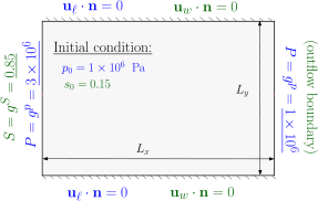
(a) Pressure-driven flow problem

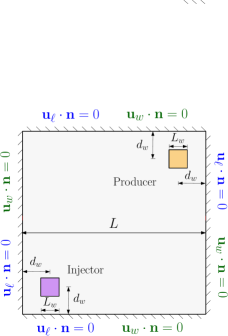
(b) Quarter five-spot flow problem

Figure 1. Pictorial description of computational domain and boundary conditions of pressure-driven flow problem and quarter five-spot problem.

4.1. Analytical problem and $h-$convergence study

We first perform an $h-$convergence study on 2D structured triangular meshes of size $h$. The computational domain is the unit square and the exact solutions are:

$$s(x,y,t)=0.4+0.4xy+\cos{t+x},$$ (4.1a)

$$p(x,y,t)=2+x^{2}y-y^{2}+x^{2}\sin{y+t}-\frac{1}{3}\cos{t}+\frac{1}{3}\cos{t+1}-\frac{11}{6}.$$ (4.1b)

We replace the right-hand side of equations (2.1)–(2.2) by body forces obtained via the manufactured solutions. Dirichlet boundary conditions are prescribed on $\partial\Omega$ on both saturation and pressure fields and the other parameters are taken as:

$$\phi=1,\quad K=1\leavevmode\nobreak\ ${\mathrm{m}}^{2}$,\quad c_{r}=c_{w}=c_{\ell}=10^{-10},\quad$$

$$\rho_{w}^{0}=\rho_{\ell}^{0}=1\leavevmode\nobreak\ $\mathrm{kg}\text{\,}{\mathrm{m}}^{-3}$,\quad\mathbf{g}=\mathbf{0},\quad\mu_{w}=\mu_{\ell}=1\leavevmode\nobreak\ $\mathrm{Pa}\text{\cdot}\mathrm{s}$.$$

Table 1 and 2 show the errors in $L^{2}$ norm and rates evaluated at $T=1$ $\mathrm{s}$ for saturation and pressure solutions. At each refinement level, the time step $\tau$ is set to $h^{2}$; and at every time instance $t$, the admissible bounds $s_{*}$ and $s^{*}$ are updated to the maximum and minimum of the exact saturation solution (4.1a). We compare the rates for three different cases of unlimited DG, limited DG (DG+FL+SL) and also the case of DG with flux limiters only (DG+FL). For both unknowns, DG and DG+FL yield expected optimal rate of $2$ in the $L^{2}$ norm whereas the application of slope limiters lead to suboptimal rates. We should highlight that the proposed flux limiter is rate-preserving and is independent of the slope limiter. Devising a rate preserving slope limiters still remains an open challenge.

Table 1. Errors in $L^{2}$ norm and convergence rates for saturation solutions at $T=1\leavevmode\nobreak\ $\mathrm{s}$$.

		DG		DG+FL		DG+FL+SL
$h$ ($\mathrm{m}$)	dofs	$\|S_{n}-s(T)||_{L^{2}(\Omega)}$	rate	$\|S_{n}-s(T)||_{L^{2}(\Omega)}$	rate	$\|S_{n}-s(T)||_{L^{2}(\Omega)}$	rate
1/2	48	$5.08\times 10^{-2}$	$-$	$4.92\times 10^{-2}$	$-$	$3.39\times 10^{-2}$	$-$
1/4	192	$1.65\times 10^{-2}$	1.62	$1.67\times 10^{-2}$	1.56	$1.35\times 10^{-2}$	1.33
1/8	768	$4.03\times 10^{-3}$	2.03	$4.05\times 10^{-3}$	2.04	$6.54\times 10^{-3}$	1.04
1/16	3072	$1.02\times 10^{-3}$	1.98	$1.02\times 10^{-3}$	1.99	$3.28\times 10^{-3}$	1.00
1/32	12288	$2.61\times 10^{-4}$	1.96	$2.61\times 10^{-4}$	1.96	$1.39\times 10^{-3}$	1.24
1/64	49152	$6.92\times 10^{-5}$	1.92	$6.92\times 10^{-5}$	1.92	$5.56\times 10^{-4}$	1.32

Table 2. Errors in $L^{2}$ norm and convergence rates for pressure solutions at $T=1\leavevmode\nobreak\ $\mathrm{s}$$.

		DG		DG+FL		DG+FL+SL
$h$ ($\mathrm{m}$)	dofs	$\|P_{n}-p(T)||_{L^{2}(\Omega)}$	rate	$\|P_{n}-p(T)||_{L^{2}(\Omega)}$	rate	$\|P_{n}-p(T)||_{L^{2}(\Omega)}$	rate
1/2	48	$2.68\times 10^{-3}$	$-$	$2.68\times 10^{-3}$	$-$	$1.74\times 10^{-3}$	$-$
1/4	192	$2.25\times 10^{-3}$	0.25	$2.25\times 10^{-3}$	0.25	$1.45\times 10^{-3}$	0.26
1/8	768	$6.74\times 10^{-4}$	1.74	$6.77\times 10^{-4}$	1.73	$5.14\times 10^{-4}$	1.50
1/16	3072	$1.80\times 10^{-4}$	1.91	$1.80\times 10^{-4}$	1.91	$1.32\times 10^{-4}$	1.96
1/32	12288	$4.55\times 10^{-5}$	1.98	$4.55\times 10^{-5}$	1.98	$3.20\times 10^{-5}$	2.04
1/64	49152	$1.14\times 10^{-5}$	1.99	$1.14\times 10^{-5}$	2.00	$8.08\times 10^{-6}$	1.99

4.2. Pressure-driven flow

In this section, we perform various pressure-driven flow problems with homogeneous and heterogeneous permeabilities to study the efficacy and robustness of limiters on capturing accurate and bound-preserving solutions. For all problems, we take a rectangular computational domain $\Omega=[0,L_{x}]\times[0,L_{y}]$ ${\mathrm{m}}^{2}$. A wetting phase is injected along the left boundary and displaces the non-wetting phase out of the domain through the right boundary. As depicted in Figure 1(a), Dirichlet boundary conditions are set to: $g^{p}=3\times 10^{6}$ $\mathrm{Pa}$ and $g^{s}=0.85$ on $\{0\}\times[0,L_{y}]$ $\mathrm{m}$; and $g^{p}=10^{6}$ $\mathrm{Pa}$ on $\{L_{x}\}\times[0,L_{y}]$ $\mathrm{m}$. Outflow boundary condition is prescribed on the right boundary for saturation and the top/bottom boundaries are set as no-flow ($j^{s}=j^{p}=0$). We note that due to the residual saturations, the exact saturation satisfies the maximum principle:

$$0.15\leq s\leq 0.85.$$

We will highlight below the behavior of the phase saturation regarding these physical bounds.

4.2.1. Example 1: Homogeneous domain

We consider a domain of length $L_{x}=100$ $\mathrm{m}$ and $L_{y}=30$ $\mathrm{m}$ with constant permeability of $K=10^{-12}$ ${\mathrm{m}}^{2}$ partitioned into structured crossed triangular meshes of size $h=10$ $\mathrm{m}$. The time step is chosen as $0.05$ days and the final time is $T=10$ days. Gravity is neglected. Figure 2 compares the saturation profiles obtained from unlimited DG, DG with only vertex-based slope limiter [Kuzmin, 2010] (i.e., DG+SL), and the proposed limited DG (i.e., DG+FL+SL) at two different time steps. It is seen that the saturation front, under all three approximations, propagates with the same speed. However, limited DG, unlike its unlimited counterparts, produces a numerical saturation that remains physically bounded and neither undershoots (blue-colored elements) nor overshoots (red-colored elements) are detected throughout the simulation. Table 3 shows the minimum and maximum values of the saturation over all time steps. While the slope limiter removes the overshoot for this simulation, there is still significant undershoot. The percentage of these overshoot and undershoot with respect to the physical range $[0.15,0.85]$ are also displayed.

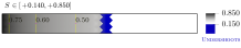
(a) DG (without limiter) at $t=5.1$ days

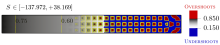
(b) DG (without limiter) at $t=10$ days

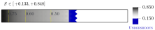
(c) DG + SL at $t=5.1$ days

(d) DG + SL at $t=10$ days

(e) DG + FL + SL at $t=5.1$ days

(f) DG + FL + SL at $t=10$ days

Figure 2. Pressure-driven flow in homogeneous domain: The evolution of saturation solutions obtained with DG (top), DG+SL (middle), and DG+FL+SL (bottom) at two different time steps. The color mapping for physical range of saturation is presented in grayscale, whereas the values below and above bounds are colored blue and red, respectively. Results suggest that DG+FL+SL, unlike the two other schemes, provides maximum-principle-satisfying solutions at all time steps.

Table 3. This table shows the efficacy of the limiting schemes when applied to the pressure-driven flow problem with homogeneous domain.

	DG		DG+SL		DG+FL+SL
	value	%	value	%	value	%
minimum saturation	-137.97	19731	0.033	16.7	0.15	0
maximum saturation	38.16	5330	0.85	0	0.85	0

4.2.2. Example 2: Heterogeneous domain

We repeat the experiment in Section 4.2.1 with an heterogeneous domain of size $L_{x}=150$ $\mathrm{m}$ and $L_{y}=100$ $\mathrm{m}$. The permeability field is composed of a highly discontinuous central block sandwiched by two buffer zones of $K=10^{-11}$ ${\mathrm{m}}^{2}$ (see Figure 3 for a description of the permeability field). The data for the central block is taken from the horizontal permeability slice number $71$ of the SPE10 benchmark model [SPE, ] that is scaled to a $100\times 100$ ${\mathrm{m}}^{2}$ grid. The domain is discretized with structured triangular mesh of size $h=5/3$ $\mathrm{m}$, time step is $\tau=1/12$ days, and total simulation time is $T=68$ days. Figure 4 shows the saturation profile under limited and unlimited DG at three different time instances $t=25$, $50$, and $68$ days. The wetting phase floods the domain from the left buffer zone toward the right buffer zone while avoiding the low permeable regions. As expected, even for highly heterogeneous domains, the proposed limited DG completely eliminates the violation of maximum principle that appeared as overshoots and undershoots in unlimited DG approximations. Figure 5 depicts the magnitude of the wetting phase velocity, $\mathbf{u}_{w}$, computed at $t=68$ days. The velocity is computed at time $t_{n}$ in each mesh element by

$$\mathbf{u}_{w}^{n}=-\lambda_{w}(S_{n})K(\nabla P_{n}-\rho_{\ell}(P_{n})\mathbf{g}).$$ (4.2)

Velocity obtained under DG with no limiters does not accurately follow the path of saturation propagation and exhibits overestimation of the magnitude of the velocity. On the other hand, the limited DG scheme eliminates these shortcomings and results in distinguishable flow paths that match those of the saturation contours. The pressure contours are shown in Figure 6 for both unlimited DG and limited DG. Both methods produce the same pressure range, but there are visible differences in the pressure field in the heterogeneous region.

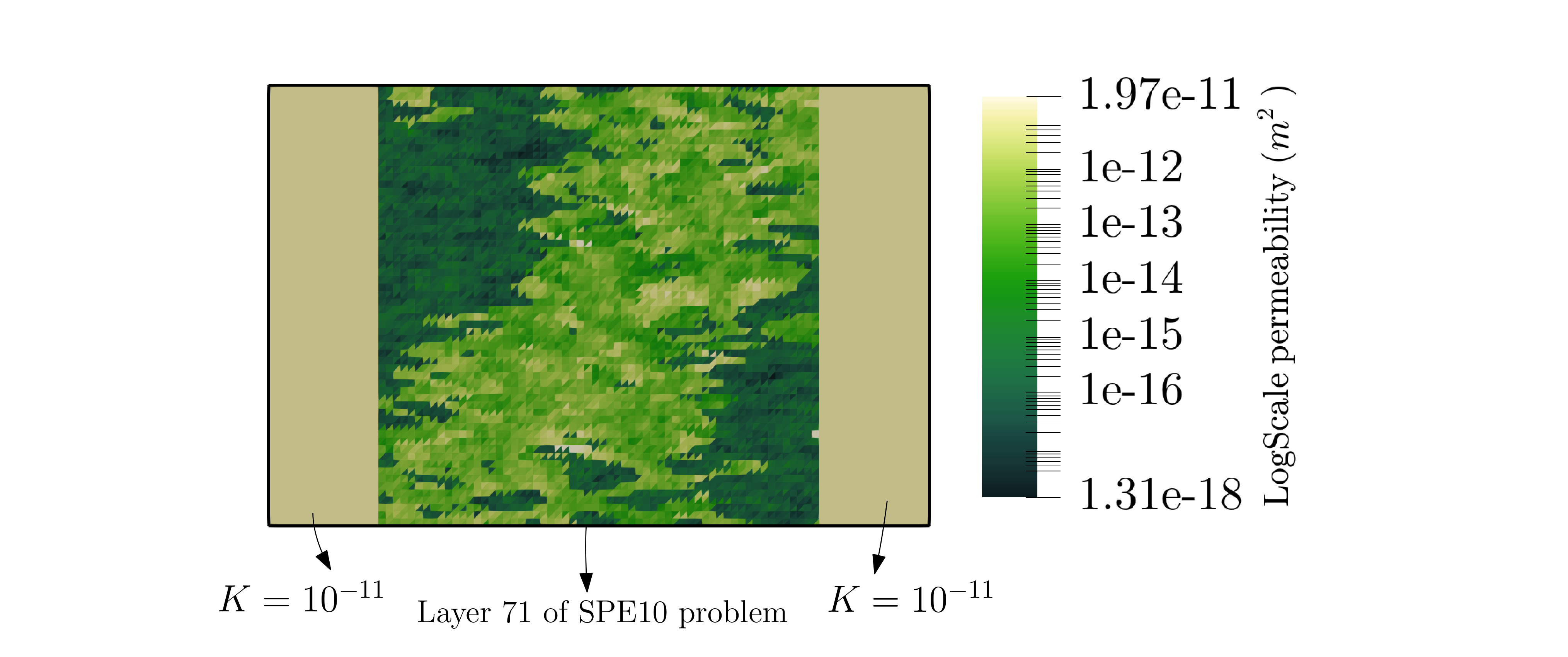
Figure 3. Pressure-driven flow in heterogeneous domain: The permeability field in the center is adopted from layer 71 of SPE10 benchmark problem. Values are shown in logarithmic scale

(a) Unlimited DG at $t=25$ days

(b) Unlimited DG at $t=50$ days

(c) Unlimited DG at $t=68$ days

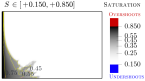
(d) Limited DG at $t=25$ days

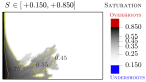
(e) Limited DG at $t=50$ days

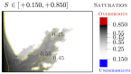
(f) Limited DG at $t=68$ days

Figure 4. Pressure-driven flow in heterogeneous domain: The evolution of saturation profile using DG scheme without limiter (top row) and with the proposed limiters (bottom row). The color mapping for physical range of saturation is presented in grayscale, whereas the values below and above bounds are colored blue and red, respectively. DG approximation give rise to noticeable violations but limited DG is capable of producing maximum-principle-satisfying results.

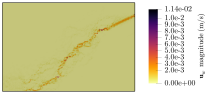
(a) Unlimited DG at $t=68$ days

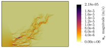
(b) Limited DG at $68$ days

Figure 5. Pressure-driven flow in heterogeneous domain: The magnitude of velocity field at final time $t=68$ days using DG scheme without limiter (left) and with limiters (right).

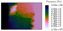
(a) Unlimited DG at $t=68$ days

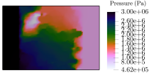
(b) Limited DG at $68$ days

Figure 6. Pressure-driven flow in heterogeneous porous media: The pressure contours at time $t=68$ days using unlimited DG (left) and limited DG (right).

4.2.3. Example 3: Non-homogeneous domain with gravitational force

We now examine the performance of our limiting scheme in the presence of gravity field. For this problem, the domain of length $L_{x}=300$ $\mathrm{m}$ and $L_{y}=100$ $\mathrm{m}$ is partitioned into a crossed triangular mesh of size $h=10/3$ $\mathrm{m}$. The gravity number $\mathrm{Gr}$ depends on the difference between phase densities. Permeability is set to $10^{-12}$ ${\mathrm{m}}^{2}$ everywhere except inside six square inclusions of length $20$ $\mathrm{m}$ centered at coordinates $(70,30)$, $(150,30)$, $(230,30)$, $(70,70)$, $(150,70)$, and $(230,70)$ $\mathrm{m}$, where the permeability is $10^{3}$ times smaller. Time step is set to $\tau=1/12$ days and the final time is $T=30$ days. The proposed DG scheme with flux and slope limiters is applied for two scenarios of $\mathrm{Gr}=0$ (i.e., no gravity) and $\mathrm{Gr}=0.4$. Figure 7 shows the saturation contours at the time $t=30$ days. In the presence of the gravitational body force, the horizontal symmetry of flow is broken and the wetting phase, which is heavier, starts to deposit at the bottom edge. As flow advances, the gravitational tongue at the bottom of domain becomes more distinct. For both problems, the limiting scheme exhibits satisfactory results with respect to the maximum principle. Pressure contours and the magnitude of the velocity field (see (4.2)) are displayed in Figure 8 and 9, respectively. The impact of gravity in both solutions is noticeable.

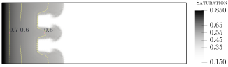
(a) No gravity; $t=30$ days

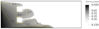
(b) With gravity; $t=30$ days

Figure 7. Pressure-driven flow in non-homogeneous domain with gravitational force: This figure shows the wetting phase saturation contours at $t=30$ days for two different cases where the gravitational force is absent (top) and is present (bottom). Both flux and slope limiter are utilized in generating results and hence no violation of maximum principle is observed.

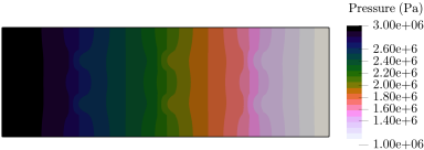
(a) Without gravitational forces; $t=30$ days

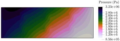
(b) With gravity body force ($\mathrm{Gr}=0.4$); $t=30$ days

Figure 8. Pressure-driven flow in non-homogeneous domain with gravitational force: This figure shows the wetting phase pressure contours at $t=30$ days for $\mathrm{Gr}=0$ and $\mathrm{Gr}=0.4$.

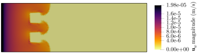
(a) No gravity; $t=30$ days

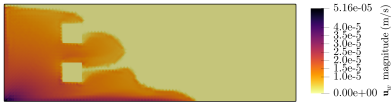
(b) With gravity; $t=30$ days

Figure 9. Pressure-driven flow in non-homogeneous domain with gravitational force: This figure shows the magnitude of wetting phase velocity solutions at $t=30$ days for $\mathrm{Gr}=0$ and $\mathrm{Gr}=0.4$.

4.3. Quarter five-spot problem

In this section, we evaluate the performance of limiters in the presence of wells. We take a square computational domain of size $L=100$ $\mathrm{m}$ with permeability of $10^{-12}$ ${\mathrm{m}}^{2}$ everywhere. The domain is partitioned into a crossed triangular mesh of size $h=2.5$ $\mathrm{m}$. As shown in Figure 1(b), no flow boundary condition is prescribed on $\partial\Omega$ and the flow is driven by injector/producers (source/sink functions) (see (2.5)). The injection saturation is set to $s_{\mathrm{in}}=0.85$ and the injection and production flow rate of wells are set to:

$$\int_{\Omega}\bar{q}=\int_{\Omega}\underline{q}=9.8437\times 10^{-4},$$ (4.3)

where $\bar{q}$ is piecewise constant on $[5,12.5]^{2}$ ${\mathrm{m}}^{2}$ and $\bar{q}=0$ elsewhere and $\underline{q}$ is piecewise constant on $[87.5,95]^{2}$ ${\mathrm{m}}^{2}$ and $\underline{q}=0$ elsewhere. Time step is set to $\tau=0.05$ days and the simulation advances up to $T=11$ days. Figure 10 depicts the wetting phase saturations at two different time of $t=4$ and $t=11$ days for unlimited DG, DG+SL, and DG+FL+SL schemes. Unlimited DG returns oscillatory non-monotone solutions and violations of the maximum principle are noticeable in the vicinity of injector and after the saturation front. The slope limiter improves the accuracy of the solution by reducing the amount of overshoot near the injection well, but falls short in generating bound-preserving solutions throughout the simulation. On the other hand, the proposed DG+FL+SL limiting scheme returns monotone solutions and fully eliminates undershoots (i.e., blue-colored cells) and overshoots (red-colored cells). Table 4 displays the minimum and maximum values of the saturations over the whole simulation, as well as the amounts of overshoot and undershoot in percentages. Figure 11 and 12 show the wetting phase pressure and the magnitude of the velocity (defined by (4.2)) under the proposed limiting scheme. As time progresses, higher pressure differences build up near the producer and hence the magnitude of the velocity increases in that region. Finally, we investigate the impact of applying slope and flux limiters on the local mass conservation properties of the DG formulation. Following (3.6), we denote by $\overline{\varphi}$ the element-wise average of a function $\varphi$. By choosing a test function equal to $1/|E|$ on one element and $0$ elsewhere, we obtain the local mass balance of an element $E\in\mathcal{E}_{h}$ at time $t_{n}$ as follows:

$$\mathcal{B}(E)= \frac{1}{\tau}\Big{(}\overline{\rho_{w}(P_{n+1})\phi(P_{n+1})S_{n+1}}-\overline{\rho_{w}(P_{n})\phi(P_{n})S_{n}}\Big{)}+\frac{1}{|E|}\sum_{e\subset\partial E}\mathcal{H}_{n+1,E}(e)$$

$$-\overline{\rho_{w}(P_{n})f_{w}(s_{\mathrm{in}})\bar{q}_{E}-\rho_{w}(P_{n})f_{w}(S_{n}|_{E})\underline{q}_{E}}.$$ (4.4)

The values of $\mathcal{B}(E)$ are displayed in Figure 13 for unlimited DG, DG+SL and DG+FL+SL at time $t=7$ days. We observe that the mass error is of the order of $10^{-9}$ everywhere except in a small neighborhood of the saturation front where the mass error increases to $10^{-5}$. The slope and flux limiters do not change the magnitude of the local mass error.

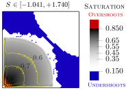
(a) Unlimited DG; $t=4$ days

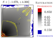
(b) Unlimited DG; $t=11$ days

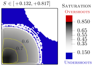
(c) DG+SL; $t=4$ days

(d) DG+SL; $t=11$ days

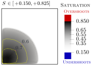
(e) DG+FL+SL; $t=4$ days

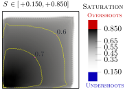
(f) DG+FL+SL; $t=11$ days

Figure 10. Quarter five-spot problem in homogeneous domain: This figure shows the saturation contours obtained with DG (top), DG+SL (middle), DG+FL+SL (bottom) at two different time steps. The proposed DG+FL+SL scheme, unlike the two other schemes, respects maximum principle throughout the simulation.

Table 4. This table shows the efficacy of the limiting schemes when applied to the quarter five-spot flow problem with homogeneous domain.

	DG		DG+SL		DG+FL+SL
	value	%	value	%	value	%
minimum saturation	-1.39	220	-0.1137	37.7	0.15	0
maximum saturation	10.51	1380	0.86	1.4	0.85	0

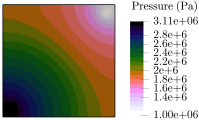
(a) Limited DG; $4$ days

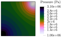
(b) Limited DG; $11$ days

Figure 11. Quarter five-spot problem in homogeneous domain: This figure shows the wetting phase pressures obtained under the proposed DG+FL+SL algorithm.

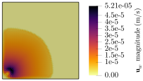
(a) Limited DG; $4$ days

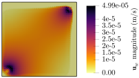
(b) Limited DG; $11$ days

Figure 12. Quarter five-spot problem in homogeneous domain: This figure shows the wetting phase velocities obtained under the proposed limiting algorithm.

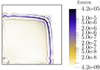
(a) Unlimited DG

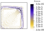
(b) DG+SL

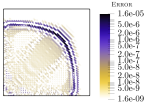
(c) DG+FL+SL

Figure 13. Quarter five-spot problem in homogeneous domain: This figure shows the element-wise mass balance error $\mathcal{B}(E)$ at time $t=7$ days. Errors remain small regardless of the scheme used.

4.4. Effect of rock and phases compressibility factors

In this section we use the limited DG scheme to study the impact of compressibility factors on pressure-driven flow problem discussed in Section 4.2.1 and the quarter-five spot problem discussed in Section 4.3. We first set the rock compressibility to take three different physical values of $3\times 10^{-10}$, $6\times 10^{-10}$, and $9\times 10^{-10}$ ${\mathrm{Pa}}^{-1}$ [Baker et al., 2015] and examine two cases of compressible phases (with $c_{w}=10^{-10}$ and $c_{\ell}=10^{-6}$) and incompressible phases (i.e., $c_{w}=c_{\ell}=0$). Other parameters and boundary conditions remain unchanged. Figure 14(a) displays the saturation solution for compressible phases along the line $y=5$ $\mathrm{m}$. We observe that the rock compressibility factor yields negligible changes in solutions. From Figures 14(b) and 15 it can be seen that the wetting phase floods the domain faster in the incompressible case than in the compressible case.

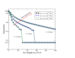
(a) Various rock compressibilites

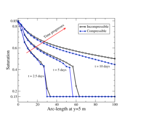
(b) Compressible vs incompressible fluid phases

Figure 14. Effect of compressibility factors for a pressure-driven flow problem:  This figure shows the evolution of saturation profiles obtained from the limited DG scheme for (a) three different rock compressibility factors with fixed $c_{w}=10^{-10}$ and $c_{\ell}=10^{-6}$ and (b) for different phase compressibility factors with fixed $c_{r}=6\times 10^{-10}$. Rock compressibility has negligible effect on solutions. It is also evident that fluid compressibility slows down the propagation of wetting phase saturation.

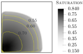
(a) Compressible case; saturation

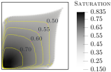
(b) Incompressible case; saturation

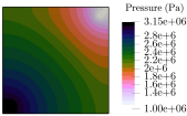
(c) Compressible case; pressure

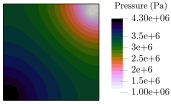
(d) Incompressible case; pressure

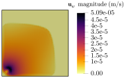
(e) Compressible case; velocity

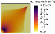
(f) Incompressible case; velocity

Figure 15. Quarter five-spot problem in homogeneous domain:  This figure compares solutions for compressible and incompressible phases obtained from limited DG scheme at $t=6.5$ days. Wetting phase fluid propagates faster for the incompressible case.

4.5. Quarter five-spot problem with a highly anisotropic permeability

Finally, to examine the capability of the proposed limiting scheme to produce a correct and bound-preserving solution for strongly anisotropic permeability fields, we present the results for the boundary-value problem illustrated in Figure 16, which was adopted from [Galindez-Ramirez et al., 2020; Nikitin et al., 2014]. The permeability matrix is defined as follows:

$$K=\begin{bmatrix}\cos\theta&-\sin\theta\\ \sin\theta&\cos\theta\end{bmatrix}\begin{bmatrix}k_{1}&0\\ 0&k_{2}\end{bmatrix}\begin{bmatrix}\cos\theta&\sin\theta\\ -\sin\theta&\cos\theta\end{bmatrix},$$ (4.5)

where principal permeabilities are set to $k_{1}=2.25\times 10^{-12}$ and $k_{2}=2.25\times 10^{-14}$. As shown in Figure 16 the permeability field is divided into four separate regions with distinct anisotropic $K$, in which the angle $\theta$ is equal to 45 degree in the bottom left and upper right parts of the domain and alternate between 0 and 90 degree in the central region. The remaining parameters are the same as in Section 4.3. Figure 17 depicts the computational results computed with the proposed limited DG scheme at three different time instances. It is clear that the limiting strategy honors the domain’s heterogeneity and anisotropy and the channel flow with stair-case shape is captured. It should be also noted that no violation of maximum principle or spurious oscillations are obtained in the solutions.

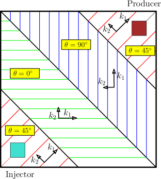
Figure 16. Quarter five-spot problem with a discontinuous full tensor and highly anisotropic permeability. Principal permeabilities are set to $k_{1}=2.25\times 10^{-12}$ and $k_{2}=2.25\times 10^{-14}$.

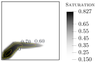
(a) $t=1.25$ days; saturation

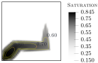
(b) $t=2.5$ days; saturation

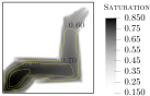
(c) $t=5$ days; saturation

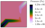
(d) $t=1.25$ days; pressure

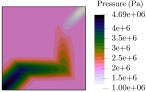
(e) $t=2.5$ days; pressure

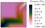
(f) $t=5$ days; pressure

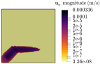
(g) $t=1.25$ days; velocity

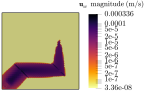
(h) $t=2.5$ days; velocity

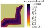
(i) $t=5$ days; velocity

Figure 17. Quarter five-spot problem in an anisotropic domain: this figure shows the computational results obtained from the limited DG scheme as time advances. The proposed scheme satisfies the maximum principle throughout the simulation. The zigzag flow pattern confirms that solutions respect the anisotropy of the domain.

4.6. A note on the solver and scheme performance

We implement the proposed computational framework using the finite element capabilities in Firedrake Project [Rathgeber et al., 2016; McRae et al., 2016; Homolya and Ham, 2016; Homolya et al., 2018, 2017] with GNU compilers. We resort to the MPI-based PETSc library [Balay et al., 2017, 2018; Dalcin et al., 2011] as the linear algebra back-end to solve the nonlinear system. We use Newton’s method with step line search technique and set the relative convergence tolerance to $10^{-6}$. At each time step, after the Newton solver convergence, we apply flux and slope limiters. Implementation of the flux limiter algorithm is discussed in Section 3.1 and the global stopping criteria for all problem sets are taken as $\epsilon_{1}=\epsilon_{2}=10^{-6}$. As for the slope limiter, we take advantage of the VertexBasedLimiter module embedded in the Firedrake project. All simulations are run on a single socket Intel i5-8257U node by utilizing a single MPI process. Codes used to perform all experiments in this paper are publicly available at msarrafj/LimiterDG [2022] repository for reproducibility.

Table 5 illustrates the Newton solver and flux limiter performance in terms of number of iterations. A few Newton iterations are needed at each time step for the convergence of either limited DG or unlimited DG approximations. It is evident that the limiters do not have a noticeable effect on the number of solver iterations. We also see that the number of flux limiter iterations is not significantly affected by the compressibility factors. However, the maximum number of iterations increases as heterogeneity, gravity, and anisotropy are added to the system. It should be noted that the reported number range for flux limiter is recorded throughout the simulation time and we observed that in fact for most time steps (over 85% to 90%), flux limiter iterations remain relatively small (less than 5 iterations).

Table 5. Number of nonlinear Newton iterations and flux limiter iterations per time step during the simulation

Problem description		Unlimited DG	Limited DG+FL+SL
		Newton’s iter. num.	Newton’s iter. num.	FL iter. num.
Sec 4.2 - Ex 1	homogeneous-bc-w/o gravity	$3-5$	$3-5$	$2-8$
Sec 4.2 - Ex 2	heterogeneous-bc-w/o gravity	$3-5$	$3-5$	$2-11$
Sec 4.2 - Ex 3	nonhomogeneous-bc-with gravity	$3-7$	$3-7$	$3-30$
Sec 4.3	homogeneous-wells-w/o gravity	$4-5$	$4-5$	$4-28$
Sec 4.5	anisotropic-wells-w/o gravity	$3-5$	$3-5$	$4-53$

5. Conclusions

We have developed a numerical method that solves for primary unknowns the wetting phase saturation and pressure of a compressible two-phase flows problem in a compressible rock matrix. A fully implicit discontinuous Galerkin scheme is augmented with post-processing flux and slope limiters for the saturation. The performance and accuracy of the method is investigated for several benchmark problems including the quarter-five spot problem. Overshoot and undershoot are completely eliminated throughout the whole simulation time. The impact of the limiters on the local mass conservation is shown to be negligible. The use of flux and slope limiters does not change the number of Newton iterations compared to the case of unlimited DG. Numerical simulations show that the limited DG scheme significantly improves the monotonicity of the saturation compared to the one obtained with the unlimited method. The limited DG method produces sharp saturation fronts with minimal numerical diffusion, and can handle anisotropic media. The method is also shown to be robust for flows under gravitational forces.

References

- [1] Website: http://www.spe.org/web/csp/datasets/set02.htm.
- Aavatsmark [2002] Ivar Aavatsmark. An introduction to multipoint flux approximations for quadrilateral grids. Computational Geosciences, 6:405–432, 2002.
- Baker et al. [2015] R. O. Baker, H. W. Yarranton, and J. L. Jensen. 7-conventional core analysis–rock properties. Practical Reservoir Engineering and Characterization, pages 197–237, 2015.
- Balay et al. [2017] S. Balay, S. Abhyankar, F. Adams M, J. Brown, P. Brune, K. Buschelman, L. Dalcin, V. Eijkhout, W. D. Gropp, D. Kaushik, M. G. Knepley, L. C. McInnes, K. Rupp, B. F. Smith, S. Zampini, H. Zhang, and H. Zhang. PETSc users manual. Technical Report ANL-95/11 - Revision 3.8, Argonne National Laboratory, 2017.
- Balay et al. [2018] S. Balay, S. Abhyankar, M. F. Adams, J. Brown, P. Brune, K. Buschelman, L. Dalcin, V. Eijkhout, W. D. Gropp, D. Kaushik, M. G. Knepley, D. A. May, L. C. McInnes, R. T. Mills, T. Munson, K. Rupp, P. Sanan, B. F. Smith, S. Zampini, H. Zhang, and H. Zhang. PETSc Web page, 2018.
- Bastian [2014] P. Bastian. A fully-coupled discontinuous Galerkin method for two-phase flow in porous media with discontinuous capillary pressure. Computational Geosciences, 18(5):779–796, 2014.
- Chen et al. [2006] Z. Chen, G. Huan, and Y. Ma. Computational methods for multiphase flows in porous media, volume 2. Siam, 2006.
- Contreras et al. [2021] F.R.L. Contreras, D.K.E. Carvalho, G. Galindez-Ramirez, and P.R.M. Lyra. A non-linear finite volume method coupled with a modified higher order muscl-type method for the numerical simulation of two-phase flows in non-homogeneous and non-isotropic oil reservoirs. Computers & Mathematics with Applications, 92:120–133, 2021.
- Dalcin et al. [2011] L. D. Dalcin, R. R. Paz, P. A. Kler, and A. Cosimo. Parallel distributed computing using Python. Advances in Water Resources, 34(9):1124–1139, 2011.
- de Carvalho et al. [2007] D.K.E. de Carvalho, R.B. Willmersdorf, and P.R.M. Lyra. A node-centred finite volume formulation for the solution of two-phase flows in non-homogeneous porous media. International journal for numerical methods in fluids, 53(8):1197–1219, 2007.
- Doyle et al. [2020] Bryan Doyle, Beatrice Riviere, and Michael Sekachev. A multinumerics scheme for incompressible two-phase flow. Computer Methods in Applied Mechanics and Engineering, 370:113213, 2020.
- Droniou [2014] J. Droniou. Finite volume schemes for diffusion equations: introduction to and review of modern methods. Mathematical Models and Methods in Applied Sciences, 24(08):1575–1619, 2014.
- Epshteyn and Riviere [2007] Y. Epshteyn and B. Riviere. Fully implicit discontinuous finite element methods for two-phase flow. Applied Numerical Mathematics, 57(4):383–401, 2007.
- Ern et al. [2010] A. Ern, I. Mozolevski, and L. Schuh. Discontinuous Galerkin approximation of two-phase flows in heterogeneous porous media with discontinuous capillary pressures. Computer methods in applied mechanics and engineering, 199(23-24):1491–1501, 2010.
- Frank et al. [2019] F. Frank, A. Rupp, and D. Kuzmin. Bound-preserving flux limiting schemes for DG discretizations of conservation laws with applications to the Cahn–Hilliard equation. Computer Methods in Applied Mechanics and Engineering, 359:112665, 2019. doi: 10.1016/j.cma.2019.112665.
- Galindez-Ramirez et al. [2020] G. Galindez-Ramirez, F.R.L. Contreras, K.D.E. Carvalho, and P.R.M. Lyra. Numerical simulation of two-phase flows in 2-D petroleum reservoirs using a very high-order CPR method coupled to the MPFA-D finite volume scheme. Journal of Petroleum Science and Engineering, 192:107220, 2020.
- Ghilani et al. [2019] M. Ghilani, E.L.H. Quenjel, and M. Saad. Positive control volume finite element scheme for a degenerate compressible two-phase flow in anisotropic porous media. Computational Geosciences, 23:55–79, 2019.
- Homolya and Ham [2016] M. Homolya and D. A. Ham. A parallel edge orientation algorithm for quadrilateral meshes. SIAM Journal on Scientific Computing, 38(5):48–61, 2016.
- Homolya et al. [2017] M. Homolya, R. C. Kirby, and D. A. Ham. Exposing and exploiting structure: optimal code generation for high-order finite element methods. Available on arXiv: 1711.02473, 2017.
- Homolya et al. [2018] M. Homolya, L. Mitchell, F. Luporini, and D. A. Ham. TSFC: a structure-preserving form compiler. SIAM Journal on Scientific Computing, 40(3):C401–C428, 2018.
- Hoteit and Firoozabadi [2008] H. Hoteit and A. Firoozabadi. Numerical modeling of two-phase flow in heterogeneous permeable media with different capillarity pressures. Advances in Water Resources, 31(1):56–73, 2008.
- Hoteit et al. [2004] H. Hoteit, Ph. Ackerer, R. Mose, J. Erhel, and B. Philippe. New two-dimensional slope limiters for discontinuous Galerkin methods on arbitrary meshes. J. Numer. Meth. Engrg., 61:2566–2593, 2004.
- Hou et al. [2016] J. Hou, J. Chen, S. Sun, and Z. Chen. Adaptive mixed-hybrid and penalty discontinuous Galerkin method for two-phase flow in heterogeneous media. J. Comput. Appl. Math., 307:262–263, 2016.
- Jamei and Ghafouri [2016] M. Jamei and H. Ghafouri. A novel discontinuous Galerkin model for two-phase flow in porous media using an improved IMPES method. Int. J. Numer. Methods Heat Fluid Flow, 26:284–306, 2016.
- Joshaghani et al. [2022] M.S. Joshaghani, B. Riviere, and M. Sekachev. Maximum-principle-satisfying discontinuous Galerkin methods for incompressible two-phase immiscible flow. Computer Methods in Applied Mechanics and Engineering, 391:114550, 2022.
- Klieber and Riviere [2006] W. Klieber and B. Riviere. Adaptive simulations of two-phase flow by discontinuous Galerkin methods. Computer Methods in Applied Mechanics and Engineering, 196:404–419, 2006.
- Krivodonova [2007] L. Krivodonova. Limiters for high-order discontinuous Galerkin methods. J. Comput. Phys., 226:879–896, 2007.
- Kuzmin [2010] D. Kuzmin. A vertex-based hierarchical slope limiter for p-adaptive discontinuous galerkin methods. Journal of Computational and Applied Mathematics, 233(12):3077–3085, 2010.
- Kuzmin [2013] D. Kuzmin. Slope limiting for discontinuous Galerkin approximations with a possibly non-orthogonal Taylor basis. Int. J. Numer. Methods Fluids, 71:1178–1190, 2013.
- Kuzmin and Gorb [2012] D. Kuzmin and Y. Gorb. A flux-corrected transport algorithm for handling the close-packing limit in dense suspensions. Journal of Computational and Applied Mathematics, 236(18):4944–4951, 2012. doi: https://doi.org/10.1016/j.cam.2011.10.019.
- McRae et al. [2016] A. T. T. McRae, G. T. Bercea, L. Mitchell, D. A. Ham, and C. J. Cotter. Automated generation and symbolic manipulation of tensor product finite elements. SIAM Journal on Scientific Computing, 38(5):25–47, 2016.
- Michel [2003] A. Michel. A finite volume scheme for the simulation of two-phase incompressible flow in porous media. SIAM J. Numer. Anal., 41:1301–1317, 2003.
- Nikitin et al. [2014] K. Nikitin, K. Terekhov, and Y. Vassilevski. A monotone nonlinear finite volume method for diffusion equations and multiphase flows. Computational Geosciences, 18(3-4):311–324, 2014.
- Rathgeber et al. [2016] F. Rathgeber, D. A. Ham, L. Mitchell, M. Lange, F. Luporini, A. T. T. McRae, G. T. Bercea, G. R. Markall, and P. H. J. Kelly. Firedrake: automating the finite element method by composing abstractions. ACM Transactions on Mathematical Software (TOMS), 43(3):24, 2016.