Tetris: A compilation Framework for VQE Applications

Abstract

Quantum computing has shown promise in solving complex problems by leveraging the principles of superposition and entanglement. The Variational Quantum Eigensolver (VQE) algorithm stands as a pivotal approach in the realm of quantum algorithms, enabling the simulation of quantum systems on quantum hardware. In this paper, we introduce two innovative techniques, namely "Tetris" and "Fast Bridging," designed to enhance the efficiency and effectiveness of VQE tasks.

The "Tetris" technique addresses a crucial aspect of VQE optimization by unveiling cancellation opportunities within the logical circuit phase of the Unitary Coupled Cluster Singles and Doubles (UCCSD) ansatz. By strategically identifying and exploiting cancellations in the quantum circuit, Tetris demonstrates a remarkable reduction up to 20% in CNOT gate counts, about 119048 CNOT gates, and 30% depth reduction compared to the state-of-the-art UCCSD compiler ’Paulihedral’. This efficiency gain contributes significantly to the overall performance enhancement of VQE computations.

In addition to Tetris, we present the "Fast Bridging" technique as an alternative to the conventional qubit routing methods that heavily rely on swap operations. The fast bridging offers a novel approach to qubit routing, mitigating the limitations associated with swap-heavy routing. By integrating the fast bridging into the VQE framework, we observe further reductions in CNOT gate counts and circuit depth, synergistically complementing the benefits achieved through Tetris. The bridging technique can achieve up to 27% CNOT gate reduction in the QAOA application.

Through a combination of Tetris and the fast bridging, we present a comprehensive strategy for enhancing VQE performance. Our experimental results showcase the effectiveness of Tetris in uncovering cancellation opportunities and demonstrate the symbiotic relationship between Tetris and the fast bridging in minimizing gate counts and circuit depth. This paper contributes not only to the advancement of VQE techniques but also to the broader field of quantum algorithm optimization.

1 Introduction

Quantum computing, a rapidly evolving field, has the potential to revolutionize the way we process information by leveraging the principles of quantum mechanics. Among the various applications of quantum computing, quantum simulation has emerged as a promising area [24, 22, 15, 12, 3, 11]. The idea of using quantum computers to efficiently solve complex problems, such as simulating the evolution of quantum systems governed by a Hamiltonian, was first proposed by Richard Feynman [10]. This concept has spurred the development of hybrid quantum-classical solutions, which merge the strengths of both computing types and offer enhanced error resistance compared to standard quantum applications. Variational Quantum Algorithms (VQA), such as the Variational Quantum Eigensolver (VQE) [21] and the Quantum Approximate Optimization Algorithm (QAOA) [9, 7, 8], stand as prime examples of these hybrid solutions utilizing quantum simulation kernels to optimize their performance.

The transformation of a Hamiltonian simulation kernel into an executable quantum circuit involves the application of the Trotter-Suzuki decomposition [32, 29]. This method facilitates the expression of the Hamiltonian as a sum of simpler elements, known as $Pauli$ $strings$. These strings can then be converted into a series of quantum gates, which constitute the quantum circuit. However, circuit synthesized in this way for quantum simulation kernels appear as extensive gate sequences in many quantum programs. It is crucial to optimize the compilation of the quantum simulation kernel. Significantly, the permutation of Pauli strings is not rigidly fixed, providing flexibility in the design of the quantum circuit. Additionally, the synthesis of a Pauli string is adaptable, leading to a reduction in the number of SWAP gates required considering the constraints of the underlying hardware architecture. Furthermore, the compilation process for a quantum simulation kernel presents substantial opportunities for gate cancellation between two consecutive Pauli strings.

Existing compilation methodologies [33, 17, 19, 26, 27, 34, 30, 23, 28] are primarily tailored for predetermined quantum circuits, characterized by a fixed structure and gate sequence. These methods, however, overlook the potential benefits that could be derived from the synthesis of Pauli strings and the inherent flexibility in their ordering. Other domain-specific compilers [16, 1, 2, 14] are primarily engineered to address the 2-local Hamiltonian problem, such as QAOA problem. While these compilers offer flexibility in gate sequencing, they do not extend this flexibility to the circuit synthesis for each individual Pauli string.

Paulihedral [18] introduces an innovative compiler framework that leverages the Pauli intermediate representation to uphold high-level semantics and constraints inherent in quantum simulation kernels. This framework incorporates scheduling passes that not only optimize circuit parallelism for superconducting backend compilation but also streamline the processes of circuit synthesis, gate cancellation, and qubit mapping.

Nonetheless, a trade-off exists between achieving maximal gate cancellation and generating hardware-friendly logical circuits. While gate cancellation can be maximized without considering hardware connectivity, this often determines the circuit structure, potentially compromising the generation of circuits that are optimally suited to the hardware. Furthermore, the pursuit of a hardware-efficient circuit synthesis could entirely preclude the possibility of gate cancellation.

To strike a balance between gate cancellation and the compilation cost for multi-qubit gates, a new compilation framework is proposed, equipped with a novel Intermediate Representation (IR), referred to as Tetris, as depicted in Fig. 1. The compilation of an individual Pauli string lacks a high-level perspective and the interconnection between Pauli strings. This absence leads to a challenging conflict between gate cancellation and the synthesis of hardware-efficient circuits. Tetris mitigates this issue by grouping a sequence of Pauli strings and allocating the identical part across those Pauli strings where the gate cancellation happens. So as the framework shown in Fig. 1, Tetris compiler starts from a scheduler that maximizes the size of identical components across two consecutive Pauli strings. Meanwhile, Tetris simplifies a group of Pauli strings, resulting in an improvement in the compilation overhead.

Reflection is another aspect of the circuit synthesis of a Pauli string that previous compilers have not fully utilized. In a synthesized circuit, the right half circuit is mirroring the left half circuit. This reflection feature provides us with a novel bridging idea for solving qubit routing problems, termed fast bridging. Traditional bridging methods require the cost of three CNOT gates to implement one remote CNOT if only one ancilla qubit is needed [25]. In contrast, fast bridging allows the execution of two corresponding remote CNOT gates at the cost of two CNOT gates and one state $|0\rangle$ ancilla qubit.

Although fast bridging imposes an additional constraint on the qubit state, this constraint is alleviated by the recently proposed mid-circuit measurement technique [23, 13]. As the circuit execution progresses, an increasing number of qubits remain idle. This implies that more qubits can be measured earlier and subsequently utilized to assist in the execution of remote CNOT gates. For instance, in the case of the LiH molecule, a relatively small molecule with only 12 qubits, the first idle qubit starts showing up at the 200/800 block, and this number increases as the execution proceeds.

The key contributions of this study can be encapsulated as follows:

• We propose a new Intermediate Representation (IR), Tetris, designed to balance gate cancellation and hardware-friendly circuit synthesis.

• Through this new IR, we simplify the Pauli string representation and enhance the efficiency of the compilation process.

• We utilize the reflection feature in circuit synthesis, leading to the proposal of a fast bridging concept that addresses the qubit routing problem.

• We adapt existing scheduling methods to maximize idle qubits and employ the mid-circuit measurement technique to support the fast bridging concept.

• We conduct experiments on six different molecules, Tetris gains 20% in CNOT gate reduction and 30% in depth reduction. In addition, the fast bridging method reduced up to 27% CNOT gates in QAOA applications.

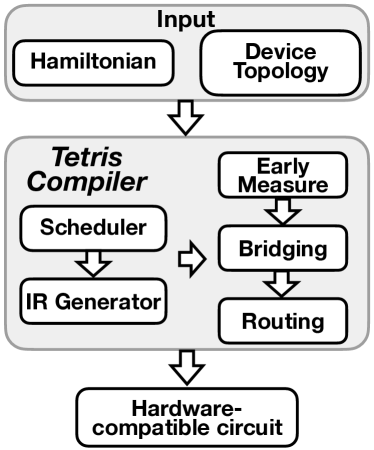
Figure 1: Overview of Tetris compiler.

2 Background

This section is dedicated to offering essential background details on quantum simulation kernels, including the process of converting a Hamiltonian into a quantum circuit. A succinct introduction to the fast-bridging concept is also provided. For a comprehensive understanding of fundamental quantum computing concepts such as qubits, gates, and circuits, we direct readers to [20].

2.1 Problem Description

In quantum computing, a simulation kernel refers to a segment of a quantum program designed to emulate a specific quantum system or process. For instance, a quantum simulation kernel could replicate the behavior of a molecule in quantum chemistry or trace the evolution of a quantum system in physics. Such kernels are commonly defined by a Hamiltonian, denoted as $H$, which mathematically represents the system or process under simulation.

Considering the simulation of a chemical molecule system as an illustrative example, the goal is to determine the least energy required to sever a chemical bond. In quantum simulation, this translates to minimizing the expectation value of the associated circuit function, given by $f(\theta)=\langle 0|U^{{\dagger}}(\theta)HU(\theta)|0\rangle$.

For the simulation of a chemical molecule system characterized by a Hamiltonian $H$, the standard approach involves transforming the system’s Hamiltonian $H$ into a summation of polynomial terms represented by Hermitian operators. The exponential of a Hermitian operator yields a unitary operator, denoted as $U=exp(it$$\sum_{j}$$h_{j}$$H_{j}$), which can depict time evolution. However, constructing a quantum circuit from this unitary operator presents challenges. The Trotter formula [32, 29] offers a prevalent method to approximate this unitary, expressed as:

$$U(t)\approx U_{Trotter}(t)=(\prod_{j=1}exp(\frac{ith_{j}H_{j}}{\rho}))^{\rho}$$ (1)

, where $\rho$ defines the precision of the approximation. Each term exp(it$h_{j}$$H_{j}$) is then expanded to an array of $exp(itP_{j}w_{j})$, where the subterm $P_{j}$ is a tensor product of Pauli operators.

The UCCSD (Unitary Coupled Cluster Singles and Doubles) ansatz [4] is a quantum circuit representation used to prepare the trial wave function for a given Hamiltonian. It is a popular choice in quantum chemistry simulations, especially when using algorithms like the Variational Quantum Eigensolver (VQE) to approximate ground state energies. With the first-order Trotter approximation ($\rho$ = 1), the UCCSD ansatz is given by

$$\begin{split}U(\theta)=\prod_{p>r}exp\{\theta_{pr}{\hat{c_{p}}^{\dagger}\hat{c_{r}}}-H.c.\}\\ \times\prod_{p>q>r>s}exp\{\theta_{pqrs}{\hat{c_{p}}^{\dagger}\hat{c_{q}}^{\dagger}\hat{c_{r}}}\hat{c_{s}}-H.c.\}\end{split}$$ (2)

, where the first product term represents the single excitation operator and the second term represent the double excitation operator. The indics r, s,and p, q represents occupied and unoccupied molecular orbitals, respectively. H.c. is the hermitian conjugate of the corresponding term.

Using the Jordan-Wigner transformation [31], we can rewrite the UCCSD unitary defined above into the product of Pauli strings. Each Pauli string is a tensor product of Pauli operators, which could be implemented in real quantum devices. The single excitation operator in Eq.(2) is rewritten into blocks of two Pauli strings and the double excitation operator is rewritten into blocks of eight Pauli strings. For the UCCSD ansatz, there is no restriction on ordering Pauli strings within a block and ordering between two blocks.

2.2 Circuit synthesis of Pauli string

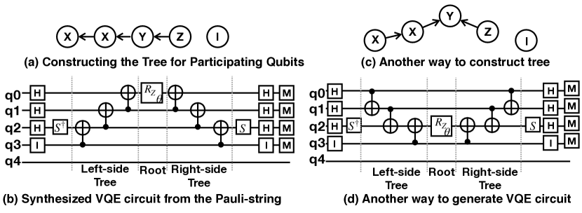
Figure 2: Two different VQE circuit constructions for the same Pauli string $I_{4}Z_{3}Y_{2}X_{1}X_{0}$. Note that I operator is an identity matrix. It does nothing, like a NOP in classical computer.

A Pauli string is a sequence composed of Pauli operators, represented as $P=\otimes_{i}$ $\sigma$_i, where $\sigma$_i $\in$ {X, Y, Z, I}. Here, $\sigma$_i specifies the type and position of the operator, with $0\leq i<n$ and n is the number of qubit. For example, consider the string $I_{4}Z_{3}Y_{2}X_{1}X_{0}$. This string requires qubits 0, 1, 2, and 3, corresponding to the indices of the qubits in the sequence. Since $I$ represents the identity operation, there’s no need to apply any operators to qubit 4.

When translating a Pauli-string description into a logical circuit, a layer of single-qubit gates is constructed based on the Pauli operators $\sigma$_i. For a qubit specified as "X" in the Pauli-string, an "H" gate is produced. If the Pauli-string indicates "Y" for a qubit, both an $H$ gate and an $S^{\dagger}$ gate are generated. No operations are performed for other characters present in the Pauli-string. A demonstrative example is provided in Fig. 2(b).

Subsequently, the circuit features a logical tree composed exclusively of CNOT gates. Any qubit, except those with the identity operator, can serve as the root of this logical tree. An illustrative tree is depicted in Fig. 2(a). Each directed edge within the tree corresponds to a CNOT gate in the circuit. The gate dependencies are also inherently defined. For instance, if edge A has its target node serving as the control node for another edge B, then A must be executed before B. This implies the existence of a dependency graph that establishes the partial ordering among all the CNOT gates.

Centrally positioned in the circuit is a single-qubit rotation gate, $Rz(\theta)$, located at the root qubit. The latter half of the circuit mirrors the initial half but with gates in the opposite sequence. All single-qubit gates in the right-side logical tree are the conjugate transpose of their corresponding gate in the left-side tree, as illustrated in Fig. 2(b). The synthesis of the circuit for the Pauli string offers flexibility. Alternate tree constructions and their corresponding circuits are depicted in Fig. 2(c) and (d).

2.3 Qubit Mapping and Fast CNOT Bridge

A logical quantum circuit is hardware-independent, allowing a two-qubit gate to be applied to two non-neighboring physical qubits. In contrast, any two-qubit gates must operate on adjacent physical qubits. One approach to address this discrepancy is by incorporating SWAP gates to dynamically adjust the qubit mapping, ensuring all two-qubit gates act on connected physical qubits. Implementing a SWAP gate requires three CNOT gates. An alternative method employs a bridge gate, composed of four consecutive CNOT gates. For both strategies, if the separation between the target physical qubits in a CNOT gate is two, then the execution of such a CNOT gate necessitates four CNOT gates.

The reflection property inherent in the Pauli string implementation offers an innovative method to execute a two-qubit gate between non-adjacent qubits. Leveraging an ancilla qubit in the |0> state, it’s possible to assist two corresponding CNOT gates positioned on either side of the Rz gate. For instance, in the initial circuit of Fig. 3, the states of q1 and q2 are unknown, they could be entangled. This circuit can be transformed into the subsequent circuit by utilizing the central qubit, which is in the $|0\rangle$ state. Proof of this transformation is also depicted in Fig. 3. Here, state $S3^{\prime}$ in the modified circuit corresponds to state $S3$ in the original, with the ancilla qubit’s state reverting to |0>.

When additional state $|0\rangle$ qubits are available to implement a distant CNOT, the fast bridging method offers pronounced enhancements. Given a separation $d$ between two target qubits of a CNOT, the SWAP approach necessitates 3(d-1) extra CNOT gates to facilitate the desired CNOT operation. On the other hand, the fast bridging technique requires merely 2(d-1) additional CNOT gates, leading to a more efficient use of CNOT gates compared to the traditional bridge strategy.

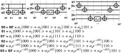
Figure 3: A fast CNOT bridge using an ancilla qubit in state |0>.

3 Opportunities and Challenges

In this section, we begin by analyzing the application scenarios of the fast bridging method and comparing the trade-offs between the SWAP and fast bridging techniques. Subsequently, the flexibility inherent in the circuit synthesis of the Pauli string is explored. Concluding the section, we discuss the challenges posed by gate cancellation and hardware-efficient circuit synthesis and introduce a new IR designed to alleviate this conflict.

3.1 Trade-off Between Fast Bridging and SWAP Insertion

In traditional quantum circuit compilers, hardware connectivity constraints are addressed by inserting SWAP gates. These gates dynamically adjust the mapping of logical qubits to physical qubits, ensuring that all two-qubit gates operate on adjacent physical qubits. However, SWAP gates introduced early in the compilation process can hinder the execution of CNOT gates later on. For instance, the SWAP(Q2, Q3) gate is added to facilitate the execution of CNOT(q3,q1) in the Pauli string $I_{5}I_{4}Z_{3}I_{2}Z_{1}Z_{0}$, as shown in Fig. 4(c). Yet, this SWAP gate also escalates the implementation cost of the second Pauli string depicted in Fig. 4(a). Consequently, the final compiled circuit for the input Pauli strings incurs an extra nine CNOT gates, leading to a total circuit depth of twelve.

However, using the fast bridging method detailed in Section 2.3, we can address the hardware connectivity constraints. In the two Pauli strings depicted in Fig. 4(a), logical qubits q2 and q4 remain unused. Assuming each qubit starts in the |0> state, then these idle qubits offer an opportunity to bridge two distant qubits. The resulting compiled circuit is illustrated in Fig. 4(d). The fast bridging method requires only four additional CNOT gates for the same Pauli string inputs, leading to a compiled circuit depth of ten.

The fast bridging technique does not consistently hold an upper hand compared to the conventional SWAP insertion approach. It encounters a pair of obstacles. First and foremost, the idle qubits utilized for the bridge must be in state |0>. In the context of VQE problems, a significant portion of Pauli strings apply non-identity Pauli operators only to a subset of qubits, thereby maintaining other qubits in state |0>. To potentially augment the use of |0> qubits in the fast bridging technique, we suggest a scheduling method for Pauli strings, which will be elaborated upon in Section 4.1.

Secondly, the choice between employing the fast bridging technique or the SWAP method hinges on the number of Pauli strings that could potentially benefit from such SWAP operations. For a sequence of s SWAP gates that can benefit a group of $k$ Pauli strings, if the following threshold T is satisfied, then the SWAP insertion method is better than the fast bridging method.

$$T=\frac{3*s}{2*\sum_{i=0}^{k}d(ps_{i})}<1$$ (3)

, where d($ps_{i}$) is the minimum distance of the bridge needed for implementing a single Pauli string. For example, for two Pauli strings in Fig. 4(a), T = 9/4, then, the fast bridging technique is better. However, as the example shown in Fig. 5, two SWAP gates required for implementing the first Pauli string resolve the hardware constraints for all following Pauli strings. In this case, T = 6/10, which means the SWAP insertion method is better than the fast bridging method.

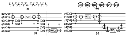
Figure 4: Fast Bridging Method is better than SWAP Insertion Method. (a) Two Pauli strings. (b) The underlying hardware. (c), (d) The compiled circuit of the input Pauli strings using the SWAP insertion method and CNOT Bridge Method respectively

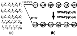
Figure 5: Fast Bridging Method worse than SWAP Insertion Method. (a) Five Pauli strings. (b) The underlying hardware with the qubit mapping before and after implementing the first Pauli string. Just two SWAP gates are required for the first Pauli string implementation, yet they are beneficial for all Pauli strings.

3.2 Circuit Synthesis of a Single Pauli String

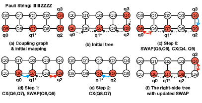
Figure 6: A full example for implementing the Pauli string IIIIIIZZZZ. (a) The coupling graph and the initial mapped active qubits. The physical qubits in red are mapped by logical qubits that has a non-identity Pauli operator on them. (b) The corresponding physical tree is generated upon the given coupling graph, the root is q1. (c)-(f) Details of circuit generation. Note that each gate is applied to physical qubits in this example. (f) The physical tree for the right-side tree with updated SWAP gates.

To compile a single Pauli string, one approach is to first synthesize the logical circuit and subsequently produce a hardware-compliant circuit tailored to the specific hardware architecture. However, this bifurcated compilation process overlooks the potential to create a hardware-optimized logical circuit that requires fewer swap gates during the qubit mapping phase.

To maintain the program’s semantics, it is necessary to synthesize the logical circuit of a single Pauli string into a tree structure known as a logical tree. The circuit execution of a logical tree follows a specific order, typically from the leaf qubits to the root qubit, resembling the transmission of signals from leaf stations to the root station.

To execute the quantum circuit on a specific architecture, the goal is to identify a subgraph within the architecture coupling graph that is isomorphic to the logical tree. This enables the circuit to be executed without the need for additional swap gates. However, finding such a subgraph can be challenging due to the variations in logical trees associated with different Pauli strings and the changing qubit mapping during circuit compilation.

In cases where it is impossible to find an exact logical tree from the coupling graph, an alternative approach is to seek a larger tree that encompasses a few additional edges along with one of the logical trees associated with the given Pauli string. This larger tree is referred to as a physical tree.

By executing the circuit within the physical tree, following the same order as logical tree execution, and replacing the extra edges with SWAP gates to account for the additional edges present. For example, for the given single pauli-string, architecture coupling graph, and initial mapping in Fig. 6(a), we generate a physical tree upon the architecture coupling graph in Fig. 6(b) with qubit q1 as the root qubit. Note that the root qubit does not have to be a mapped qubit, since one of the mapped qubits would be swapped to the root qubit eventually. Fig. 6(c)-(e) present the details of gates execution at each step for the left-side tree. Fig. 6(f) presents the physical tree for the mirror part with different SWAP insertion. The logical tree structure has to be symmetric on both sides, the SWAP inserted does not have such restriction.

3.3 Circuit Synthesis of Multiple Pauli Strings

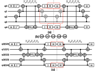
Figure 7: Gate Cancellation and limitation from the hardware connectivity. (a) The synthesized circuit for two consecutive Pauli strings, achieving the maximum number of gate cancellations. (b) The underlying hardware coupling graph. (c) Compiled circuit using hardware-efficient synthesis that does not include extra SWAP gates. Only four single-qubit gates are canceled.

3.3.1 Gate cancellation

Transitioning from the compilation of a single Pauli string to the compilation of multiple Pauli strings, the adaptability of circuit synthesis presents us with an additional opportunity for circuit optimization, Gate cancellation. When two consecutive Pauli strings possess more than one qubit sharing the same Pauli operator, at least two CNOT gates can be canceled. While some single-qubit gates might also be canceled, our focus remains on two-qubit gate cancellation, as it has a higher error rate and execution time compared to a single-qubit gate. For instance, in the two provided Pauli strings depicted in Fig. 7(a), there are three qubits with the Z Pauli operator. By meticulously synthesizing the circuit for these two Pauli strings, we can achieve a maximum of four CNOT gate cancellations and four single-qubit gate cancellations.

However, the ability to cancel gates might be restricted by the underlying hardware connectivity. As noted in Sec. 3.2, given the qubit mapping, the goal of circuit compilation is to find a hardware-compatible circuit. This circuit should require the fewest SWAP gates in accordance with the underlying architecture. For instance, considering the same pair of Pauli strings in Fig.7, the compiled circuit that aligns with the hardware coupling in Fig.7(b) is displayed in Fig.7(c). In this particular circuit, only four single-qubit gates are canceled. Yet, circuit synthesis designed for gate cancellation might be oblivious to the hardware connectivity. This oversight can result in a synthesized circuit demanding additional SWAP gates. With the identical qubit mapping seen in Fig.7(c), the pre-synthesized circuit in Fig.7(a) calls for a SWAP gate for those long-distance CNOT gates, specifically CNOT(q0, q4).

3.3.2 New Pauli IR, Tetris

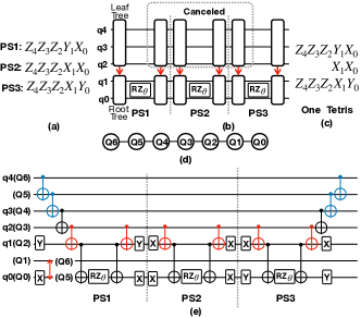
Figure 8: New Pauli IR. (a) A group of Pauli strings. (b) Gates are canceled on the leaf trees among three Pauli strings. (c) An illustration of new IR. (d) The underlying hardware coupling graph. (e) The compiled circuit of new IR with a SWAP gate and bridge CNOT gates. The single qubit gates are represented by the corresponding Pauli operators. The gates in blue are bridging gates and the red CNOT gates are the gate between two subtrees.

To retain the capability of gate cancellation while simultaneously minimizing the cost of circuit compilation, we introduce a new Pauli Intermediate Representation (IR), referred to as Tetris. A Tetris symbolizes a group of Pauli strings that share some common Pauli operators across a subset of qubits. The design of UCCSDs makes the similarity between two Pauli strings high and provides the opportunity for Tetris to include multiple Pauli strings.

Within a Tetris, each Pauli string still upholds a tree structure on either side of the root qubit. On each side, the original tree is bifurcated into two components: the leaf tree and the root tree, linked by a directional edge that connects the two subtrees. This edge represents a CNOT gate with the control qubit coming from the leaf tree and the target qubit from the root tree. The leaf tree comprises qubits that share the same Pauli operators across the Pauli strings, while the root tree houses the remaining qubits. For instance, in the three Pauli strings shown in Fig.8(a), qubits q2, q3, and q4 share the same Pauli operators, Pauli-Z; hence, the leaf tree for each Pauli string incorporates those qubits. The root qubit of a single Pauli string is selected from the root tree. The generation procedure of this structure is shown in Fig.8(b), and an illustration of this structure can be found in Fig.8(c).

Due to gate dependencies, the cancellation of CNOT gates between two Pauli strings must proceed from the gates on the leaf qubits to the gates on qubits that are closer to the root qubit. For example, four CNOT gates are canceled from the leaf qubits as shown in Fig. 7(a). Within the Tetris structure, as long as the leaf trees have identical structures, gates on the leaf trees can be canceled. Simultaneously, Tetris maintains the high-level Pauli string abstraction, facilitating circuit synthesis that takes into account the underlying hardware connectivity. Fig. 8(e) details the compiled circuit for the Pauli strings in Fig. 8(a) in relation to the hardware in Fig. 8(d). There are eight CNOT gates canceled from those leaf trees. Due to cancellations between the leaf trees, SWAP gates are needed for the leaf tree may not benefit many Pauli strings. Therefore, we utilize the fast bridging method, incurring only the cost of two additional CNOT gates for the remote gates in the leaf trees in Fig. 8(d). Regarding the CNOT gates on the root tree, it is more advantageous to insert SWAP gates as they can be of benefit to more Pauli strings.

4 Methodology

In this section, we introduce how we build our compilation framework. Tetris is starting from a scheduler that adapts the scheduler proposed in Paulihedral to achieve parallelism in block scheduling. Then we modify the block scheduling to maximize the opportunities for fast bridging. After the order of blocks is decided, we start grouping Pauli strings and simplify the Pauli string representation as a new IR with the guarantee of gate cancellation. Lastly, we synthesize the circuit with respect to the underlying hardware for the new IR.

4.1 Bridging-oriented scheduling

The block scheduling in our framework adapts the scheduler proposed in Paulihedral for the compilation in the superconducting backend. All Pauli strings are ordered in the lexicographic ordering. While this scheduling is beneficial to the gate cancellation, it did not take the qubit reuse into consideration. Since the fast bridging method requires the state of ancilla qubit has to be $|0\rangle$, we need to measure qubits that already finished all of their jobs as early as possible.

To optimize the use of fast bridging, we aim for qubits in the state $|0\rangle$ to manifest both early and frequently. We begin by sorting qubits based on the count of Identity operators associated with them. The qubit with the highest number of Identity operators, indicating the most idle time, is labeled as $q_{max}$. We then prioritize Pauli strings with non-identity operators to ensure the early measurement of this $q_{max}$ qubit. For Pauli strings that have non-identity operators on $q_{max}$, we arrange them lexicographically to facilitate effective gate cancellation. For the subsequent Pauli strings, we identify the next $q_{max}$ qubit and repeat the process.

4.2 New IR Generation for Gate Cancellation

Once the Pauli strings are appropriately arranged, it is worth discussing the size of one Tetris. A Teris consists of a sequence of Pauli strings, as the example shown in Fig. 8. It separates each tree of a Pauli string into two subtrees. The leaf tree only contains qubits sharing the same Pauli operators across Pauli strings in the Tetris and the root tree contains the remaining qubits, including the root qubit. All leaf trees could be canceled in the logical circuit, except the first one and the last one. If we include more Pauli strings in a Tetris, more gate cancellation is guaranteed.

However, increasing the size of a Tetris can amplify discrepancies among Pauli strings. This can lead to an enlarged root tree, which is counterproductive for gate cancellation. For example, if the Teris in Fig. 8 includes one more Pauli string, $Z_{4}Z_{3}X_{2}Y_{1}I_{0}$, then the new Tetris would arrange q0, q1, and q2 into the root tree resulting in only four CNOT cancellation for the first three Pauli strings. The result is shown in Fig. 9. The gates guaranteed to be canceled in Fig. 8 is eight. By default, we set one block of Pauli string as a Tetris. Then we try to include more Pauli strings. If the newly added Pauli string would not decrease the size of the existing leaf trees, we include this Pauli string, otherwise, we stop adding Pauli strings and start solving the qubit routing problem.

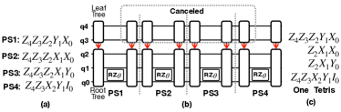
Figure 9: A Tetris with Four Pauli strings. Only six CNOT gates can guarantee to be canceled.

4.3 Circuit Synthesis with Respect to Hardware

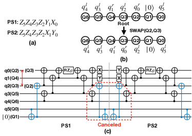
Figure 10: A concrete example of implementing Tetris compiler. (a) Two Pauli strings. (b) The coupling graph and qubit mapping. Physical qubit Q3 is selected as the center for the root tree. (c) The detail of compiled circuit. Six CNOT gates are canceled.

Algorithm 1 Circuit Synthesis

1:procedure Circuit_Synthesis($G_{coupling}$, $\pi$, $q^{r}$,$q^{l}$)

2:     $circuit$ = {}

3:     $tree$ = {}

4:     // Find a center and the shortest path from a $q^{r}_{i}$ to the center.

5:     $center$, $paths$ = findCenter($G_{coupling}$, $\pi$, $q^{r}$)

6:     for $q^{r}_{i}$ $\in$ $q^{r}$ do

7:         circuit.insert(SWAP($\pi(q^{r}_{i})$, paths($\pi(q^{r}_{i})$)))

8:         tree.insert($q^{r}_{i}$)

9:     end for

10:     // Find the shortest path from a $q^{l}_{j}$ to $q^{r}$

11:     $paths$ = findPath($G_{coupling}$, $\pi$, $q^{r}$, $q^{r}$)

12:     for $q^{l}_{j}$ $\in$ $q^{l}$ do

13:         circuit.insert(SWAP($\pi(q^{l}_{j})$, paths($\pi(q^{l}_{j})$)))

14:         tree.insert($q^{r}_{i})$))

15:     end for

16:     for leaf in tree do

17:         $circuit$.insert(CNOT(leaf, tree(leaf).getparent))

18:         tree.remove(leaf)

19:     end for

20:     return $circuit$

21:end procedure

The process of circuit synthesis for a Tetris differs from that of a Pauli string. Due to the division within the logical tree, the connectivity constraints of the root tree must be addressed earlier, even though its corresponding circuit is synthesized later. Prioritizing the synthesis of the circuit for the leaf tree is a logical step. This approach ensures that gate cancellations between successive leaf trees remain unaffected by the root tree.

To guarantee the cancellation between two leaf trees, one way is to make sure all data qubits in the root tree are mapped together, such that the mapping of those qubits would not be moved and avoid interrupting the gate cancellation between leaf trees. For the efficient grouping of all root-tree qubits, we first identify a central point within the hardware coupling graph, $G_{coupling}$, among the qubits $\pi(q^{r}{i})$. Here, $\pi$ represents the current qubit mapping, and $q^{r}$ denotes the set of qubits in the root tree. Subsequently, we introduce SWAP gates to cluster all qubits $q^{r}{i}$ around this center. It’s worth noting that the central point doesn’t necessarily have to be mapped by a data qubit $q^{r}_{i}$, as a data qubit will eventually be swapped into this position. For instance, in Fig. 10(b), we employ a SWAP(Q2, Q3) gate to ensure all $q^{r}$ are mapped in proximity to the root qubit.

Next, we proceed with the synthesis of the circuit for the leaf tree. Initially, we organize the qubits $q^{l}_{j}$ in the leaf tree based on their proximity to the root tree. Following this, we introduce SWAP gates to shift the qubit $q^{l}_{j}$ that has a smaller distance to a root tree qubit. This process continues until all $q^{l}$ qubits are linked to the root tree. Subsequently, as we synthesize the circuit for the leaf tree, we incorporate the CNOT gate. The qubit further from the root tree is selected as the control qubit, while the one closer to the root serves as the target. This procedure is reiterated until CNOT gates have been applied to all $q^{l}_{j}$ qubits. The same steps are then applied to $q^{r}$. The corresponding pseudocode is detailed in Algorithm 1, with a practical illustration provided in Fig. 10.

Bridge insertion

is considered in the process of the circuit synthesis for the leaf tree. As we discussed in Section 3.1, the fast bridging method has the advantage over the SWAP insertion method only when a SWAP gate benefits few Pauli strings. In the process of circuit synthesis for the leaf tree, we already decided on the routing paths that $q^{l}$ will move along with. In these paths, if existing qubits are in state $|0\rangle$, we consider that qubits have a Pauli operator Z on them. Such that, we would apply CNOT gates on those ancilla qubits. For example, we insert bridging CNOT gates in Fig. 10(c) between $q^{l}_{5}$ and $q^{l}_{2}$, highlighted in blue.

5 Evaluation

In this section, we provide a detailed analysis of our method by contrasting it with state-of-the-art approaches, Paulihedral[18] for the VQE and QAOA applications. We analyze the effects of individual passes and make comparisons in various dimensions, including circuit depth, two-qubit gate count, gate cancellation ratio (GCR), and the occurrence of the bridge.

5.1 Experiment Setup

Backend

The compiler framework introduced in this paper focuses on near-term superconducting backends, specifically targeting IBM’s architecture as the backend. The architecture’s size is adjusted according to the size of the input problem.

Metric

We evaluate the effectiveness of our framework using the following metrics: circuit depth, CNOT gate count, total gate count, gate cancellation ratio (GCR), the occurrence of the bridge, and circuit compilation time. Circuit depth refers to the length of the critical path in the compiled circuit, correlating with the overall duration of the circuit. It’s preferable to have a smaller circuit depth, as this can help minimize decoherence error. When calculating circuit depth, we break down a SWAP gate into three CNOT gates. Single-qubit gates are disregarded in this calculation since their duration is much shorter compared to CNOT gates, and they are more likely to be overshadowed by the execution of CNOT gates.

The two-qubit gate count is the total number of CNOT gates in the compiled circuit, encompassing both the original circuit gates, those decomposed from the added SWAP gates, and bridging gates. Since two-qubit gate errors are prevalent in accumulated gate errors, fewer gate counts signify fewer accumulated errors.

At the same time, we also showcase the ratio of original CNOT gates that have been canceled (GCR), along with the number of bridging CNOT gates, to illustrate the effectiveness of our optimization passes. We only apply the bridging method in the leaf tree, more bridging indicates more overall CNOT gate saving compared with the SWAP insertion method. Since our new IR group and simplify a sequence of Pauli strings, we compare the compilation overhead against the baseline.

Baselines

We primarily contrast our method with the specialized framework for quantum simulation kernels, Paulihedral with the gate-count-orientated scheduler [18]. Recognized as the state-of-the-art in VQE problem compilation, Paulihedral not only refines the circuit compilation from the high-level intermediate representation (Pauli string) but also leverages the adaptability of circuit synthesis and gate cancellation. The gate parallelism in Paulihedral compilation relies on the Qiskit with highest optimization level 3.

Benchmarks

We have chosen benchmarks of various sizes and applications, including the VQE UCCSD ansatzes [4] available in six different sizes. These benchmarks were generated using Qiskit. We have constructed the Hamiltonians for ten distinct molecules (LiH, BeH2, CH4, MgH2, LiCl, CO2) utilizing the PySCF software package. The target quantum hardware is ibm_ithaca, with a 65-qubit heavy hexagon structured coupling map. A comprehensive overview of these benchmarks is provided in Table 1.

Table 1: Benchmarks

Benchmarks	#Qubits	#Pauli String	#CNOT	#Single
LiH	12	640	8064	4992
BeH2	14	1488	21072	11712
CH4	18	4240	73680	33600
MgH2	22	8400	173264	66752
LiCl	28	17280	440960	137600
CO2	30	20944	568656	166848

Implementation Details

We implement our compiler with Qiskit library with optimization level 3 on Intel(R) Core(TM) i9-10900 CPU @ 2.80GHz - 20 cores computer. We consider Jordan-Wigner (JW) [4], and Bravyi-Kitaev (BK) [31] transformers. If no declared explicitly, all data shown in the paper is using the Jordan-Wigner transformer. By default, The size of one Tetris is set to one block of Pauli strings. In the Jordan-Wigner transformer, the shape of each Pauli string in a block is the same. The shape means the location of identity Pauli operators. For another transformer, the shape of Pauli strings in a block is similar as well. So, when we increase the size of a Tetris, we add whole blocks to it.

5.2 Overall comparison between Tetris and Paulihedral

The overall comparison with Paulihedral is shown in Table 2. In this table, we conduct the experiments with two different transformers, Jordan-Wigner (JW) [4], and Bravyi-Kitaev (BK) over six benchmarks. The first two columns for each method are compilation time. The first one is the compilation time of the proposed method itself and the second column is the time consumed by Qiskit. Columns #CNOT, #Sinlge, and #Total stand for the number of gate count respectively. #Total is the summation of #CNOT and #Sinlge gate count. Depth is the circuit depth generated by Qiskit. In general, Tetris outperforms Paulihedral. Tetris has up to 26.77% and 20.91% improvement in CNOT gate count; 15.25% and 10.13% improvement in total gate count; and 30.66% and 26.10% improvement in circuit depth.

Table 2: Comparison against Paulihedral

		Paulihedral						Tetris						Tetris +bridging
Trans.	Bench.	Time(s)	Qsk.T(s)	#CNOT	#Single	#Total	Depth	Time(s)	Qsk.T(s)	#CNOT	#Single	#Total	Depth	Time(s)	Qsk.T(s)	#CNOT	#Single	#Total	Depth
JW	LiH	0.56	23.47	5300	3926	9226	6156	0.36	6.76	5457	4324	9781	6325	0.30	6.55	5467	4327	9794	6336
	BeH2	1.17	58.75	15075	10334	25409	16033	0.64	69.17	12489	10518	23007	14313	0.71	28.62	12471	10518	22989	14332
	CH4	4.23	216.72	44901	27009	71910	46493	1.70	85.85	36082	30480	66562	40450	1.92	87.22	35899	30071	65970	40321
	MgH2	8.04	1147.97	90291	52449	142740	97086	3.98	153.38	76527	61112	137639	82043	3.04	154.85	75358	60846	136204	81664
	LiCl	22.10	3061.64	225277	115991	341268	245737	8.38	497.08	169973	124602	294575	175134	8.64	510.54	169823	124590	294413	175856
	CO2	23.94	4590.26	284065	142481	426546	306362	11.13	638.12	208019	153853	361872	212663	8.94	485.89	208622	152892	361514	212420
BK	LiH	0.38	17.28	10074	4689	14763	10790	0.42	17.76	9679	4954	14633	10478	0.36	17.37	9690	4947	14637	10480
	BeH2	0.73	40.16	22057	10845	32902	23140	0.78	32.96	19440	12827	32267	19773	0.79	33.84	19484	12824	32308	19797
	CH4	2.48	158.75	64163	36569	100732	61473	1.73	82.69	61485	40632	102117	57567	2.31	107.89	62228	42800	105028	56438
	MgH2	5.03	393.61	142160	71341	213501	139653	4.54	178.31	127598	81063	208661	121406	4.03	297.98	125441	85066	210507	116989
	LiCl	10.51	743.66	292658	155304	447962	285789	8.94	553.24	256162	173599	429761	234680	8.86	531.26	256336	173027	429363	234058
	CO2	11.75	1143.68	384969	176719	561688	381186	10.85	769.84	305997	201291	507288	283676	9.56	826.43	304458	200358	504816	281702

5.2.1 Gate Cancellation Comparison

Compared with Pauliheral, the main advantage of Tetris is Tetris guarantees the CNOT gate cancellation between Pauli strings. As the result shown in Fig. 11, Tetris has a better CNOT gate cancellation ratio than Paulihedral. The x-axis is the benchmark, from left to right, the size of the molecule is increasing and the size of the corresponding circuit is also increasing. The Y-axis stands for the CNOT gate cancellation ratio, higher is better. The cancellation ratio is calculated by the following:

$$ratio=\frac{canceled\_gate\_count}{original\_circuit\_gate\_count}$$ (4)

From this figure, we can see that with the size of the benchmark growing, the cancellation ratio can reach up to 70%. In terms of CNOT gate count, Tetris could make 119048 CNOT gates canceled.

The single-qubit gate cancellation in Tetris is worse than in Paulihedral, the comparison is shown Fig. 12. This is mainly due to the scheduler in Paulihedal places all Pauli strings in the lexicographic ordering. This increases the similarity between consecutive Pauli strings and maximizes the single-qubit gate cancellation.

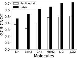
Figure 11: Cancellation Ratio cnot.

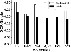
Figure 12: Cancellation Ratio single.

5.3 Effect of Different Transformer

Bravyi-Kitaev transformer is another popular transformer that maps fermionic operators in UCCSD ansatz to Pauli operators. To show the compatibility of Tetris, we conduct experiments with Bravyi-Kitaev transformer against Paulihedral over six benchmarks. The result is shown in Table 3. Each entry in this table represents the improvement over the baseline. For example, the depth of LiH compiled by Tetris is -312. This means the circuit compiled by Tetris has 312 reduction in depth. The same for the number of CNOT reductions. For this transformer, we can achieve up to 99484 depth reduction and 80511 CNOT gate count reduction.

Table 3: Comparison against Paulihedral with BK mapper

	Tetris		Tetris +bridging
Bench.	Depth	#CNOT	Depth	#CNOT
LiH	-312	-395	-310	-384
BeH2	-3367	-2617	-3343	-2573
CH4	-3906	-2678	-5035	-1935
MgH2	-18247	-14562	-22664	-16719
LiCl	-51109	-36496	-51731	-36322
CO2	-97510	-78972	-99484	-80511

5.4 Effect of Size of Tetris

The size of a single Tetris is adjustable. Since the similarity of Pauli strings in one block is high, so we try to include two blocks or three blocks in one Tetris. The corresponding result is shown in Table. 4. In this table, the column GCR Imp. stands for the difference between GCR-CNOT ratio of Tetris-2-blocks with the default Tetris, and the difference between GCR-CNOT ratio of Tetris-3-blocks with the default Tetris. The minus sign means the GCR-CNOT ratio is decreased for that setup. As we expected, once we increase the size of Tetris, the discrepancy between Pauli strings is also increased, resulting in the size of leaf tree decreased and the CNOT gate cancenllation ratio reduced.

Table 4: Size of Tetris Analysis

	Tetris-2-blocks			Tetris-3-blocks
Bench.	Depth	#CNOT	GCR Imp.	Depth	#CNOT	GCR Imp.
LiH	6731	5547	4.1%	7691	6332	-2.1%
BeH2	16726	15195	-6.2%	18156	17173	-0.6%
CH4	45783	41202	-1.5%	50862	44788	-2.1%
MgH2	91648	83550	-1.1%	104392	99320	-0.5%
LiCl	195648	184655	-2.2%	220923	212576	-1.1%
CO2	238780	229364	-2.0%	275455	265024	-0.5%

5.5 Bridging Analysis

In this section, we discuss the performance of bridging optimization. As the result shown in Table, 2, for both transformers, Tetris with bridging has better performance than both Paulihedral and Tetris. However, the improvement is not significant. For the experiment with the Jordan-Wigner transformer, we present the number of bridge gates added in Table 5. Each bridge gate stands for one ancilla qubits is used and two CNOT gate appears in both left and right tree of a single Pauli string. While the larger benchmarks provide more bridging opportunities, the briding gate count is trivial. The main reason is that Pauli strings generated from the UCCSD ansatz have high similarity. This makes SWAP gates inserted can benefit more Pauli strings.

Table 5: Bridging Count Analysis

Bench.	LiH	BeH2	CH4	MgH2	LiCl	CO2
#Bridge	5	19	47	92	126	155

5.5.1 Improvement from Bridging in QAOA

While there are instances where bridging’s effectiveness is limited within the context of UCCSD, owing to significant similarities among individual sets of Pauli strings, the bridging indicates substantial benefits for QAOA, particularly in the case of simple and concise QAOA circuits. These circuits consist of multiple group of ZZ gates, each group displaying minimal resemblance to others. This dissimilarity among groups uniquely positions bridging to excel. Look at Table 6 for example. We generated two distinct graph types utilizing the networkx library: ’power’ and ’random’. Specifically, the ’power’ graph (power(n, m, p)) was crafted using networkx’s powerlaw_cluster_graph(n, m, p) function, wherein ’n’ represents node count, ’m’ signifies the number of randomized edges introduced for each new node, and ’p’ denotes the likelihood of triangular additions following the integration of random edges. On the other hand, the ’random’ graph (random(n)) was generated through networkx’s erdos_renyi_graph(n, p) method, utilizing ’n’ and ’p’ in a similar context.

Starting from the uppermost entry and progressing downwards, we systematically vary the number of nodes n from 15 to 20. Notably, Power(n, 4, 0.05) are the most intricate and deepest circuits among Power(n, 2, 0.05) and Random(n). Conversely, Random(n) are the simplest and shortest circuits. You can see as those QAOA circuits get simpler and shorter in depth, a corresponding CNOT gate count improvement becomes apparent, rising from ~10% to ~30%.

Table 6: Bridge Improvement in QAOA

Bench.	PH	PH + bridging	#CNOT Imp.
Power(15, 4, 0.05)	373	331	11.26%
Power(16, 4, 0.05)	379	343	9.50%
Power(17, 4, 0.05)	389	345	11.31%
Power(18, 4, 0.05)	463	410	11.45%
Power(19, 4, 0.05)	444	403	9.23%
Power(20, 4, 0.05)	513	461	10.14%
Power(15, 2, 0.05)	280	233	16.79%
Power(16, 2, 0.05)	302	259	14.24%
Power(17, 2, 0.05)	297	241	18.86%
Power(18, 2, 0.05)	280	246	12.14%
Power(19, 2, 0.05)	317	267	15.77%
Power(20, 2, 0.05)	318	269	15.41%
Random(15)	56	40	28.57%
Random(16)	47	35	25.53%
Random(17)	156	117	25.00%
Random(18)	73	53	27.40%
Random(19)	182	144	20.88%
Random(20)	93	71	23.67%

5.6 Scalability Analysis

In this section, we represent the scalability analysis over three methods. In Fig. 13, the x-axis is the benchmark and the y-axis is the compilation time in seconds. The compilation time includes the compilation time from the proposed method and the optimization time consumed by Qiskit. In this figure, Tetris compiler is faster than Paulihedral. This is due to Tetris canceling most of the CNOT gates in the leaf trees between two consecutive Pauli strings. It lowers the workload in the qubit routing stage and alleviates the pressure from constant updating the qubit mapping. Subsequently, the optimization time cost from Qiskit is reduced as well.

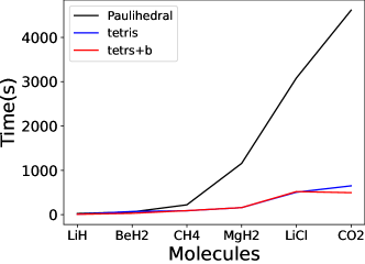
Figure 13: Scalability Analysis.

6 Related Work

Prior compilation techniques [33, 17, 19, 26, 27, 34, 30, 23, 28] were primarily tailored for quantum circuits with predefined structures and logical gates. Their primary objective was to address the qubit mapping challenge by incorporating swap gates, taking into account qubit and gate error rates, without the necessity for gate commutation. This is because, in conventional quantum circuits, altering the gate sequence could easily compromise the program’s semantics. Subsequently, domain-specific compilers [16, 1, 14] emerged to handle QAOA circuits, which permit flexible gate sequencing. However, these compilers overlook the potential advantages offered by the adaptability of circuit synthesis in VQA applications.

Paulihedral [18] stands out as the pioneering framework to employ a Pauli string intermediate representation, effectively maintaining the high-level semantics and constraints inherent in quantum simulation kernels. This framework introduces innovative scheduling passes that seamlessly integrate circuit synthesis, gate cancellation, and qubit mapping, thereby optimizing the performance of quantum simulation kernels. Notably, Paulihedral does not delve deeply into the intricacies arising from simultaneous gate cancellation and circuit synthesis. Recognizing this gap, Tetris identifies the conflict and introduces a novel intermediate representation to address it. Additionally, Tetris leverages the reflection characteristic in circuit synthesis and puts forth an innovative qubit routing approach, complemented by a mid-circuit measurement technique.

Varsaw [5] aims to enhance circuit fidelity by addressing measurement errors in Variational Quantum Algorithms. Building upon the foundation set by JigSaw [6], VarSaw pinpoints and rectifies redundancies inherent in the JigSaw method, specifically targeting spatial overlaps among subsets from varied VQA circuits and temporal overlaps among different VQA iterations. By strategically tackling these overlaps, VarSaw achieves a notable reduction in computational overhead. While Tetris seeks fidelity enhancement by refining gate count and circuit depth, VarSaw’s approach is distinct and complementary to our research.

7 Conclusion

We introduce Tetris, a novel compilation framework designed for quantum simulation kernels. Tetris presents a unique Intermediate Representation (IR) that simultaneously addresses gate cancellation and optimizes circuit synthesis for hardware efficiency. Furthermore, Tetris offers an innovative qubit routing technique, fast bridging, leveraging the reflection characteristic within the circuit of quantum simulation ansatz. The fast bridging method is advocated by the mid-circuit measurement technique to minimize the compilation overhead and improve the qubit utilization.

References

- [1] Mahabubul Alam, Abdullah Ash-Saki, and Swaroop Ghosh. Circuit compilation methodologies for quantum approximate optimization algorithm. In 2020 53rd Annual IEEE/ACM International Symposium on Microarchitecture (MICRO), pages 215–228, 2020.
- [2] Mahabubul Alam, Abdullah Ash Saki, and Swaroop Ghosh. An efficient circuit compilation flow for quantum approximate optimization algorithm. In Proceedings of the 57th ACM/EDAC/IEEE Design Automation Conference, DAC ’20. IEEE Press, 2020.
- [3] Frank Arute, Kunal Arya, Ryan Babbush, Dave Bacon, Joseph C. Bardin, Rami Barends, Andreas Bengtsson, Sergio Boixo, Michael Broughton, Bob B. Buckley, David A. Buell, Brian Burkett, Nicholas Bushnell, Yu Chen, Zijun Chen, Yu-An Chen, Ben Chiaro, Roberto Collins, Stephen J. Cotton, William Courtney, Sean Demura, Alan Derk, Andrew Dunsworth, Daniel Eppens, Thomas Eckl, Catherine Erickson, Edward Farhi, Austin Fowler, Brooks Foxen, Craig Gidney, Marissa Giustina, Rob Graff, Jonathan A. Gross, Steve Habegger, Matthew P. Harrigan, Alan Ho, Sabrina Hong, Trent Huang, William Huggins, Lev B. Ioffe, Sergei V. Isakov, Evan Jeffrey, Zhang Jiang, Cody Jones, Dvir Kafri, Kostyantyn Kechedzhi, Julian Kelly, Seon Kim, Paul V. Klimov, Alexander N. Korotkov, Fedor Kostritsa, David Landhuis, Pavel Laptev, Mike Lindmark, Erik Lucero, Michael Marthaler, Orion Martin, John M. Martinis, Anika Marusczyk, Sam McArdle, Jarrod R. McClean, Trevor McCourt, Matt McEwen, Anthony Megrant, Carlos Mejuto-Zaera, Xiao Mi, Masoud Mohseni, Wojciech Mruczkiewicz, Josh Mutus, Ofer Naaman, Matthew Neeley, Charles Neill, Hartmut Neven, Michael Newman, Murphy Yuezhen Niu, Thomas E. O’Brien, Eric Ostby, Bálint Pató, Andre Petukhov, Harald Putterman, Chris Quintana, Jan-Michael Reiner, Pedram Roushan, Nicholas C. Rubin, Daniel Sank, Kevin J. Satzinger, Vadim Smelyanskiy, Doug Strain, Kevin J. Sung, Peter Schmitteckert, Marco Szalay, Norm M. Tubman, Amit Vainsencher, Theodore White, Nicolas Vogt, Z. Jamie Yao, Ping Yeh, Adam Zalcman, and Sebastian Zanker. Observation of separated dynamics of charge and spin in the fermi-hubbard model, 2020.
- [4] Panagiotis Kl. Barkoutsos, Jerome F. Gonthier, Igor Sokolov, Nikolaj Moll, Gian Salis, Andreas Fuhrer, Marc Ganzhorn, Daniel J. Egger, Matthias Troyer, Antonio Mezzacapo, Stefan Filipp, and Ivano Tavernelli. Quantum algorithms for electronic structure calculations: Particle-hole hamiltonian and optimized wave-function expansions. Physical Review A, 98(2), aug 2018.
- [5] Siddharth Dangwal, Gokul Subramanian Ravi, Poulami Das, Kaitlin N. Smith, Jonathan M. Baker, and Frederic T. Chong. Varsaw: Application-tailored measurement error mitigation for variational quantum algorithms, 2023.
- [6] Poulami Das, Swamit Tannu, and Moinuddin Qureshi. JigSaw: Boosting fidelity of NISQ programs via measurement subsetting. In MICRO-54: 54th Annual IEEE/ACM International Symposium on Microarchitecture. ACM, oct 2021.
- [7] Edward Farhi, Jeffrey Goldstone, and Sam Gutmann. A quantum approximate optimization algorithm. arXiv preprint arXiv:1411.4028, 2014.
- [8] Edward Farhi, Jeffrey Goldstone, Sam Gutmann, and Leo Zhou. The quantum approximate optimization algorithm and the sherrington-kirkpatrick model at infinite size. Quantum, 6:759, 7 2022.
- [9] Edward Farhi and Aram W Harrow. Quantum supremacy through the quantum approximate optimization algorithm. arXiv preprint arXiv:1602.07674, 2016.
- [10] Richard P Feynman. Simulating physics with computers. International Journal of Theoretical Physics, 21(6/7), 1982.
- [11] I. M. Georgescu, S. Ashhab, and Franco Nori. Quantum simulation. Rev. Mod. Phys., 86:153–185, Mar 2014.
- [12] Cornelius Hempel, Christine Maier, Jonathan Romero, Jarrod McClean, Thomas Monz, Heng Shen, Petar Jurcevic, Ben P. Lanyon, Peter Love, Ryan Babbush, Alá n Aspuru-Guzik, Rainer Blatt, and Christian F. Roos. Quantum chemistry calculations on a trapped-ion quantum simulator. Physical Review X, 8(3), jul 2018.
- [13] Fei Hua, Yuwei Jin, Yanhao Chen, Suhas Vittal, Kevin Krsulich, Lev S. Bishop, John Lapeyre, Ali Javadi-Abhari, and Eddy Z. Zhang. Exploiting qubit reuse through mid-circuit measurement and reset, 2023.
- [14] Yuwei Jin, Jason Luo, Lucent Fong, Yanhao Chen, Ari B. Hayes, Chi Zhang, Fei Hua, and Eddy Z. Zhang. A structured method for compilation of qaoa circuits in quantum computing, 2022.
- [15] Stephen P. Jordan, Keith S. M. Lee, and John Preskill. Quantum algorithms for quantum field theories. Science, 336(6085):1130–1133, jun 2012.
- [16] Lingling Lao and Dan E. Browne. 2qan: A quantum compiler for 2-local qubit hamiltonian simulation algorithms. In Proceedings of the 49th Annual International Symposium on Computer Architecture, ISCA ’22, page 351–365, New York, NY, USA, 2022. Association for Computing Machinery.
- [17] Gushu Li, Yufei Ding, and Yuan Xie. Tackling the qubit mapping problem for nisq-era quantum devices. In Proceedings of the Twenty-Fourth International Conference on Architectural Support for Programming Languages and Operating Systems, pages 1001–1014. ACM, 2019.
- [18] Gushu Li, Anbang Wu, Yunong Shi, Ali Javadi-Abhari, Yufei Ding, and Yuan Xie. Paulihedral: a generalized block-wise compiler optimization framework for quantum simulation kernels. In Proceedings of the 27th ACM International Conference on Architectural Support for Programming Languages and Operating Systems, pages 554–569, 2022.
- [19] Prakash Murali, Jonathan M. Baker, Ali Javadi-Abhari, Frederic T. Chong, and Margaret Martonosi. Noise-adaptive compiler mappings for noisy intermediate-scale quantum computers. In Proceedings of the Twenty-Fourth International Conference on Architectural Support for Programming Languages and Operating Systems, ASPLOS ’19, pages 1015–1029, New York, NY, USA, 2019. ACM.
- [20] Michael A. Nielsen and Isaac L. Chuang. Quantum Computation and Quantum Information: 10th Anniversary Edition. Cambridge University Press, 2010.
- [21] Alberto Peruzzo, Jarrod McClean, Peter Shadbolt, Man-Hong Yung, Xiao-Qi Zhou, Peter J. Love, Alán Aspuru-Guzik, and Jeremy L. O’Brien. A variational eigenvalue solver on a photonic quantum processor. Nature Communications, 5(1), jul 2014.
- [22] David Poulin, M. B. Hastings, Dave Wecker, Nathan Wiebe, Andrew C. Doherty, and Matthias Troyer. The trotter step size required for accurate quantum simulation of quantum chemistry, 2014.
- [23] QISKit: Open Source Quantum Information Science Kit. https://https://qiskit.org/.
- [24] Sadegh Raeisi, Nathan Wiebe, and Barry C Sanders. Quantum-circuit design for efficient simulations of many-body quantum dynamics. New Journal of Physics, 14(10):103017, oct 2012.
- [25] Marcos Yukio Siraichi, Vinícius Fernandes dos Santos, Caroline Collange, and Fernando Magno Quintão Pereira. Qubit allocation. Proceedings of the 2018 International Symposium on Code Generation and Optimization, 2018.
- [26] Marcos Yukio Siraichi, Vinícius Fernandes dos Santos, Caroline Collange, and Fernando Magno Quintão Pereira. Qubit allocation as a combination of subgraph isomorphism and token swapping. Proc. ACM Program. Lang., 3(OOPSLA), October 2019.
- [27] Marcos Yukio Siraichi, Vinícius Fernandes dos Santos, Sylvain Collange, and Fernando Magno Quintão Pereira. Qubit allocation. In Proceedings of the 2018 International Symposium on Code Generation and Optimization, pages 113–125. ACM, 2018.
- [28] Seyon Sivarajah, Silas Dilkes, Alexander Cowtan, Will Simmons, Alec Edgington, and Ross Duncan. tket: a retargetable compiler for nisq devices. Quantum Science and Technology, 6(1):14003, nov 2020.
- [29] Masuo Suzuki. General theory of fractal path integrals with applications to many-body theories and statistical physics. Journal of Mathematical Physics, 32(2):400–407, 02 1991.
- [30] Bochen Tan and Jason Cong. Optimal layout synthesis for quantum computing. In 2020 IEEE/ACM International Conference On Computer Aided Design (ICCAD), pages 1–9. IEEE, 2020.
- [31] Andrew Tranter, Peter J. Love, Florian Mintert, and Peter V. Coveney. A comparison of the bravyi–kitaev and jordan–wigner transformations for the quantum simulation of quantum chemistry. Journal of Chemical Theory and Computation, 14(11):5617–5630, sep 2018.
- [32] H. F. Trotter. On the product of semi-groups of operators. Proceedings of the American Mathematical Society, 10(4):545–551, 1959.
- [33] Chi Zhang, Ari Hayes, Longfei Qiu, Yuwei Jin, Yanhao Chen, and Edd Z. Zhang. Time-optimal qubit mapping. In Proceedings of the Twenty-Sixth International Conference on Architectural Support for Programming Languages and Operating Systems, ASPLOS ’21, Virtual, 2021. ACM.
- [34] Alwin Zulehner, Alexandru Paler, and Robert Wille. Efficient mapping of quantum circuits to the IBM QX architectures. In 2018 Design, Automation & Test in Europe Conference & Exhibition (DATE), pages 1135–1138. IEEE, 2018.