Inferring Actual Treatment Pathways from Patient Records

Abstract

Objective: Treatment pathways are step-by-step plans outlining the recommended medical care for specific diseases; they get revised when different treatments are found to improve patient outcomes. Examining health records is an important part of this revision process, but inferring patients’ actual treatments from health data is challenging due to complex event-coding schemes and the absence of pathway-related annotations. The objective of this study is to develop a method for inferring actual treatment steps for a particular patient group from administrative health records — a common form of tabular healthcare data — and address several technique- and methodology-based gaps in treatment pathway-inference research.

Methods: We introduce Defrag, a method for examining health records to infer the real-world treatment steps for a particular patient group. Defrag learns the semantic and temporal meaning of healthcare event sequences, allowing it to reliably infer treatment steps from complex healthcare data. To our knowledge, Defrag is the first pathway-inference method to utilise a neural network (NN), an approach made possible by a novel, self-supervised learning objective. We also developed a testing and validation framework for pathway inference, which we use to characterise and evaluate Defrag’s pathway inference ability, establish benchmarks, and compare against baselines.

Results: We demonstrate Defrag’s effectiveness by identifying best-practice pathway fragments for breast cancer, lung cancer, and melanoma in public healthcare records. Additionally, we use synthetic data experiments to demonstrate the characteristics of the Defrag inference method, and to compare Defrag to several baselines, where it significantly outperforms non-NN-based methods.

Conclusions: Defrag offers an innovative and effective approach for inferring treatment pathways from complex health data. Defrag significantly outperforms several existing pathway-inference methods, but computationally-derived treatment pathways are still difficult to compare against clinical guidelines. Furthermore, the open-source code for Defrag and the testing framework are provided to encourage further research in this area.

1 Introduction

Treatment pathways are step-by-step plans outlining the recommended interventions for treating a group of patients with a particular disease [35]. For example, a breast cancer treatment pathway may specify suitable interventions, such as surgery or chemotherapy, and their order, like pre- or post-surgical chemotherapy [5]. Treatment pathways are a central component of clinical pathway research, a discipline that spans a patient’s entire healthcare journey, from initial screening to end-of-life care. Treatment pathways, which specifically address therapeutic interventions, minimise variability in clinical practice, and ultimately lead to improved patient outcomes [32, 36, 35].

In practice, an individual patient’s actual treatments can deviate from best-practice treatment pathways due to demographic, geographic, and socioeconomic factors [11, 12]. Examining the health records of a patient cohort to determine their actual pathway of treatments offers valuable insights into treatment patterns that can lead to improved treatment pathways [13, 52]. For instance, identifying the most effective cancer treatments can shape treatment pathway recommendations. However, using health records to develop treatment pathways is challenging due to the interplay of many clinical factors [6, 48]. Issues such as patient traits (e.g., comorbidities or genetic predispositions) and environmental factors (e.g., resource availability or practitioner experience) create inconsistencies in health records, making identifying the cohort’s actual treatment pathway tough.

To address these challenges, techniques such as process mining [10, 3, 26, 24, 25] and probabilistic models [55, 56, 21, 19, 46, 47, 20] are commonly used to identify pathway-related concepts in healthcare data. Process mining studies primarily focus on identifying simpler structures like common event sequences (e.g., event B follows event A), but struggle to capture dynamic and unstructured medical processes [50]. Probabilistic methods are capable of inferring more complex patterns (e.g., event B follows event A with a given probability); however, they face limitations in addressing long-range temporal dependencies, high dimensionality, rare or noisy events, and may not accurately portray the influence of past events on future decisions.

This study aims to enhance treatment pathway inference research by introducing a new method, Defrag, to infer actual treatment pathways from administrative health records (AHRs), a common form of tabular healthcare data. Defrag comprises a Transformer neural network (NN) that is trained on AHRs using a novel, self-supervised training objective called the semantic-temporal learning objective (STLO). Defrag infers pathways in two steps: 1) the Transformer generates a joint semantic-temporal encoding of AHR events, and 2) Defrag applies network inference to determine sequential correlations between clusters of encoded events, uncovering actual treatment pathways. Defrag excels at capturing complex, long-range dependencies, modelling non-linear relationships, learning context-aware event representations, and demonstrating robustness to noise. Using self-supervised learning without prior pathway-specific labels or pre-trained encodings, Defrag can adapt to various healthcare settings, accommodate data variations across regions, and remain relevant as medical practices change.

We also present a technique for generating synthetic AHRs, which we utilise for testing pathway inference methods, including Defrag. Synthesising AHRs from ground-truth pathways enables quantitative evaluation of Defrag’s effectiveness in inferring actual treatment pathways. It helps characterise the strengths and weaknesses of Defrag while also allowing benchmarking and comparisons with alternative approaches. This technique also helps assess Defrag’s performance in relation to various data factors, such as treatment consistency, code-set vocabulary size, and pathway complexity. This approach is currently the only method for quantitatively evaluating pathway inference methods.

We demonstrate Defrag by identifying fragments of best-practice treatment pathways for breast cancer [5], lung cancer [41], and melanoma [29] from the publicly available MIMIC-IV dataset [22]. Furthermore, we show in synthetic experiments that Defrag is substantially more accurate than several baselines at inferring synthetic pathways. We also open-source our code to facilitate the reproducibility of our results and research iteration.

We summarise the significance of this paper as follows:

Problem: Inferring actual treatment pathways from complex administrative health records (AHRs) is challenging due to variations in patient comorbidities, responses, and resource availability.

What is Already Known: Existing methods struggle with capturing dynamic and unstructured medical processes, hindering pathway inference. Limited open-source data and evaluation techniques further impede reproducibility and validation.

What this Paper Adds: We introduce Defrag, a novel method utilising a Transformer neural network for inferring treatments in AHRs. We also present a novel method for pathway inference validation using synthetic data. Defrag significantly outperforms existing methods and identifies best-practice treatment patterns for three cancer types in public AHRs.

2 Background and Related Work

Administrative health records (AHRs) are temporal, tabular datasets collected for administrative purposes, such as insurance and billing. These records capture event logs of specific treatment activities, such as diagnoses and procedures. However, numerous clinical factors make pathway inference challenging [6, 48]. Such factors include a patient’s comorbidities, genetic predispositions, and treatment responses, as well as other healthcare factors such as resource availability, practitioner experience, and geographic, socioeconomic, and cultural factors.

Process mining has been investigated for discovering treatment pathways in AHRs [10, 3, 26, 24, 25]. Process mining is a method of uncovering rule-based patterns in event logs which assumes the underlying process occurs in a structured manner [1]. This assumption is a known limitation of process mining in AHRs, particularly for human-centric clinical pathways [17]. AHRs often produce unstructured patterns driven by the decisions of individual patients and healthcare practitioners rather than strict business processes [23, 34, 50]. Other studies have applied related techniques to directly infer temporal patterns between events in AHRs for heart failure and EHR workflow patterns [49, 54]. These approaches struggle to account for semantically similar events or long-range temporal dependencies, which are essential components of treatment pathways, and thus these factors limit the applicability of process mining for pathway inference [50, 17].

Probabilistic models such as Markov chains [55, 56], Latent Dirichlet Allocation (LDA) or other topic models [21, 19, 46, 47], and Hidden Markov Models [20] may better identify clinical pathways in unstructured, human-centric AHRs. Unlike process mining, these methods can capture more abstract processes. However, they often oversimplify AHRs (e.g., removing the temporal component) or impose model constraints (e.g., the Markov condition) [15], limiting their ability to discover non-linear temporal patterns or account for the impact of past events on future decisions in unstructured and noisy AHRs.

The need for open-source data and code limits AHR-based clinical pathway research. Except for one study [10], all research relies on closed-source datasets, and none share their code. Moreover, only some studies validate data-derived clinical pathways against real-world pathways, which is challenging due to the semantic gap between clinically-developed and computationally-derived treatment pathways. Furthermore, AHRs do not capture clinical pathway-related concepts, and clinical pathways need to be computer-interpretable, making inferred pathways difficult to validate [31].

In this study, we apply sequence-based neural networks (NNs) to model AHRs for pathway inference. NN-based methods (e.g., Word2Vec [30] and Transformers [42]) are highly applicable for processing natural language, a form of data that resembles the unstructured sequences of treatment events typically found in AHRs. NN-based methods have been applied successfully to AHR analysis (e.g., Med2Vec [7], and MiME [8]), but they have yet to be used for inferring treatment pathways.

To enhance the accessibility of pathway inference methods, we offer open-source code for our methodology. Additionally, we develop a synthetic data generation method to facilitate performance evaluation and comparison of pathway inference methods. We also demonstrate results on the publicly available MIMIC-IV AHR dataset [22].

3 Method

This section outlines our methodological contributions in two parts. Section 3.1 pertains to the pathway defragmentation approach and Section 3.2 pertains to synthetic AHR data generation.

3.1 Pathway Defragmentation Method

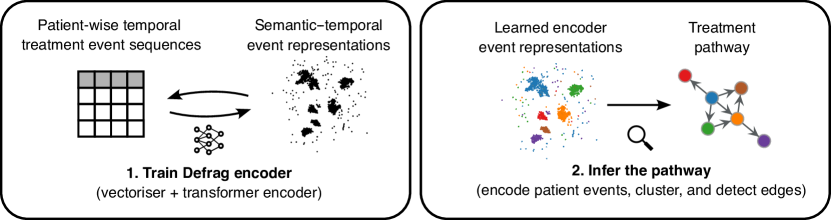
Figure 1: Pathway defragmentation (Defrag) is a 2-step process for inferring actual treatment pathways from administrative health records (AHR). For the first step, we use patients’ health records to train an event encoder that maps categorical treatment event codes to a semantic-temporal numerical representation via a Transformer neural network and a novel self-supervised learning objective. In the second step, we encode the patients’ treatment events, cluster the encoded event representations, and infer a graph of the treatment clusters using the temporal information in the raw event sequences.

We introduce Defrag, a novel technique for identifying treatment pathways in AHRs. Defrag comprises two components, as illustrated in Figure 1. The first component generates a temporally contextualised encoding of AHR events, learning patterns of events frequently occurring in close temporal proximity across numerous patients, resulting in a mapping that preserves temporal closeness. For instance, though distinct, anaesthetic and endoscopy procedures should have similarly encoded representations, as they are often utilised concurrently.

The second component infers a pathway by partitioning the encoded event space into clusters, identifying macro-scale temporal relationships between partitions. An example would be the frequent occurrence of diagnostic procedures before therapeutic procedures. The clustering groups similar events, and the temporal relationships contribute to the pathway graph formation.

3.1.1 AHR Data Representation

AHRs are typically tabular, with rows $i\in\{1,\dots,n\}$ representing different events over time, and columns ${X^{(1)},\dots,X^{(k)}}$ for different variables (e.g., diagnosis codes and procedure codes). We seek to represent $n$ events observations from an arbitrary number of variables $k$ as a single matrix. This process is shown in Figure 2 (left).

For any patient, consider the sequence $x^{(k)}_{1},x^{(k)}_{2},\dots,x^{(k)}_{n}$ of $n$ events (rows) from a single categorical variable $X^{(k)}$. If the cardinality of $X^{(k)}$ is $m^{(k)}$ , then the sequence can be represented as an $n\times m^{(k)}$ matrix $\mathbf{O}^{(k)}$ of $n$ one-hot vectors. Additionally, consider several variables $X^{(1)},X^{(2)},\dots,X^{(k)}$; we represent a sequence of each variable as an $n\times m^{(k)}$ matrix similarly.

For each variable $X^{(1)},X^{(2)},\dots,X^{(k)}$, we use multilayer perceptrons to learn mappings $f_{1},f_{2},\dots,f_{k}$ from the one-hot encoded vectors to vectors of size $D$, which are applied event-wise to $\mathbf{O}^{(1)},\mathbf{O}^{(2)},\dots,\mathbf{O}^{(k)}$ to yield $n\times D$ shaped sequence matrices for each variable, denoted as $\mathbf{S}^{(1)},\mathbf{S}^{(2)},\dots,\mathbf{S}^{(k)}$. By concatenating the vectors for each event in the sequence along the columns, $n$ observations from several variables $k$ can be represented as a single $n\times kD$ matrix. While numerical features are less common in AHRs, they too can be included in the concatenation. Finally, another event-wise mapping $f_{\mathbf{vec}}$ reduces the dimension of the concatenated vectors (length $kD$) to $d$. The result is a single sequence matrix of event vectors $\mathbf{S_{vec}}$ of shape $n\times d$, which numerically represents all $n$ observations from all $k$ variables.

The benefit of this approach is threefold: 1) it significantly reduces the dimensionality of the one-hot encoded features, reducing their redundancy and mitigating the computational burden of the subsequent sequence model (see Section 3.1.2), 2) it enables the conversion of categorical data common in AHRs to numerical data required by NNs, and 3) it does not preclude numerical features or pre-trained encodings (e.g., Med2Vec [7]) from being utilised, which can also be included in the $f_{\mathbf{vec}}$ mapping.

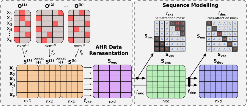
Figure 2: The flow of AHR events’ transformation into encoded/decoded vector representations. Categorical variables are one-hot encoded (red), then mapped to fixed-length vectors by $f_{k}$ and concatenation (orange), then to a vector of size $d$ by $f_{\mathbf{vec}}$ to produce $\mathbf{S_{vec}}$ (purple). Then, the transformer encoder $f_{\mathbf{enc}}$ maps $\mathbf{S_{vec}}$ to $\mathbf{S_{enc}}$ (green), and finally the transformer decoder $f_{\mathbf{dec}}$ maps $\mathbf{S_{vec}}$ and $\mathbf{S_{enc}}$ to $\mathbf{S_{dec}}$ (blue). The attention masks in the encoder and decoder for $n=6$ events are depicted in the upper-right. $w=2$ for the encoder’s windowed mask. “A” and “M” indicate positions which can and cannot attend respectively.

3.1.2 Sequence Modelling

The vectorised events in $\mathbf{S_{vec}}$ only contain semantic information, e.g., a vector representing anaesthesia use in the ICU. This section discusses how to create new vector representations of events that contain both semantic and temporal context. e.g., a patient is anaesthetised in the ICU for an endoscopy. We use the semantic event vectors $\mathbf{X}_{i,\mathbf{vec}}$ in $\mathbf{S_{vec}}$ to learn new event vectors that contain semantic and temporal information using a Transformer encoder-decoder architecture [42]. The encoder $f_{\mathbf{enc}}$ and decoder $f_{\mathbf{dec}}$ are trained to generate new $d$-shaped vectors for all $n$ events in $\mathbf{S_{vec}}$.

We diverge from the original Transformer configuration in [42] in three ways. 1) Defrag’s Transformer is trained with a unique, self-supervised objective that emphasises learning temporal features (Section 3.1.3). 2) We relative (instead of absolute) positional encoding [39, 18]. 3) We adjust the attention masks in the encoder and decoder. Specifically, the encoder uses windowed self-attention mask in the encoder, with each event attending to $w$ of its neighbours on either side. A lower $w$ leads to more event-level encodings, while a higher $w$ results in more patient-level encoding. We also mask diagonal positions in the decoder’s self- and cross-attention masks to prevent information from flowing directly between the model’s input and output and to promote encoder and decoder to learn distinct features. The attention masks are depicted in the upper-right corner of Figure 2, and Appendix A analyses the implications of these decisions, including the effect of $w$ on the learned event representations.

3.1.3 Training and Loss Function

We train the parameters $\theta$ of Defrag’s Transformer to generate joint semantic-temporal representations of events. Supervised learning is not possible since AHRs contain no semantic-temporal labels nor any other treatment pathway-specific attributes or annotations. Instead, we explored several popular self-supervised learning objectives – e.g., auto-encoding, Barlow-twins [53], SimCSE [14] – but all were suboptimal for pathway inference (see Appendix C).

We designed a novel objective called the semantic-temporal learning objective (STLO) to optimise $\theta$. STLO is a contrastive objective that encourages the Transformer to learn encoded representations of events that expose their semantic and temporal qualities . Such information is critical for pathway inference since some events in the sequence will be related to the same treatment (e.g., procedure and anaesthetic events during surgery), while some events in the sequence might be a part of different treatments (e.g., surgery and then chemotherapy).

$\mathcal{L}_{\mathrm{STLO}}$ consists of three components: closeness ($clo$), separation ($sep$), and consistency ($con$). These components are used to separate a sequence of events into two temporally contiguous groups. Clo (Equation 3) measures the within-group distances – it is minimised when the representations of such events are similar. Sep (Equation 4) measures the between-group distance – it is minimised when the representations between the two groups are dissimilar. Finally, con (Equation 5) can be interpreted as a regularisation term – it is minimised when the distribution of representations across groups does not vary significantly.

$\mathcal{L}_{\mathrm{STLO}}$ is computed as follows: for $\mathbf{S_{rep}}$, which can be either $\mathbf{S_{enc}}$ or $\mathbf{S_{dec}}$, the sequence of $n$ event vectors is used to compute a sequence of $n-1$ Euclidean distances $\mathbf{dist}_{\mathrm{rep}}$ between adjacent representations. From these distances, we compute $\mathrm{dist}_{\mathrm{mean}}$ and $\mathrm{dist}_{\mathrm{max}}$ as follows:

$$\mathrm{dist}_{\mathrm{mean}} =\frac{1}{n-1}\sum_{i=1,i\neq\operatorname*{argmax}{\mathbf{dist}}}^{n-1}(\mathbf{dist}_{\mathrm{rep},i}),$$ (1)

$$\mathrm{dist}_{\mathrm{max}} =\max_{i=1}^{n-1}{\left(\mathbf{dist}_{\mathrm{rep},i}\right)}.$$ (2)

where $0<\mathrm{dist}_{\mathrm{mean}}\leq\mathrm{dist}_{\mathrm{max}}$. Then, we compute $clo$, $sep$ and $con$:

$$clo =\mathrm{dist}_{\mathrm{mean}}/\min{(\mathrm{dist}_{\mathrm{max}}+\epsilon,\zeta)}$$ (3)

$$sep =1-\tanh{\left(\left(\mathrm{dist}_{\mathrm{max}}-\mathrm{dist}_{\mathrm{mean}}\right)/\eta\right)}$$ (4)

$$con =\operatorname*{\sigma}_{i=1,i\neq\operatorname*{argmax}{\mathbf{dist}}}^{n-1}{(\mathbf{dist}_{\mathrm{rep},i})}$$ (5)

where $\zeta$ and $\eta$ are constants which are used to equilibrate the scales of $clo$ and $sep$, and $\epsilon$ is a small positive value to prevent division by zero. We find $\zeta=10,\eta=20$, and $\epsilon=10^{-8}$ to be suitable for all our experiments. We choose these specific formulations because they are simple to compute and effective in practice . To combine these components, we compute $\mathcal{L}_{\mathrm{STLO}}$ on $\mathbf{S_{enc}}$ and $\mathbf{S_{dec}}$ separately, and take the loss at each training step as $clo_{\mathbf{dec}}+sep_{\mathbf{dec}}+con_{\mathbf{enc}}$. Figure 3 shows how minimising $clo+sep$ both minimises the within-group distances $\mathrm{dist}_{\mathrm{mean}}$, while simultaneously maximising the between-group distance $\mathrm{dist}_{\mathrm{max}}$, thus separating the sequence into two groups.

Figure 3: A contour plot showing the loss landscape for the sum of the $clo$ and $sep$ components of $\mathcal{L}_{\mathrm{STLO}}$, which vary for different values of $d_{\mathrm{mean}}$ and $d_{\mathrm{max}}$.

During training, contiguous segments from patients’ event logs are sampled as sequences of length $n$. Sequences shorter than $n$ events are padded to the right, but the STLO is computed only on the valid portion of each sequence.

Notably, $\mathcal{L}_{\mathrm{STLO}}$ computes $clo$ and $sep$ using Defrag’s decoded sequence representation $\mathbf{S_{dec}}$, while the semantic-temporal representations used for pathway inference are the encoder’s output $\mathbf{S_{enc}}$. We highlight that $\mathbf{S_{dec}}$ is not used for pathway inference since STLO’s inductive biases may not lead to useful representations. For example, sequences containing more or fewer than two kinds of treatment groups would be valid yet incompatible with STLO. However, these inductive biases are not placed on the encoder; it too must learn both semantic and temporal information since the decoder cannot rely on such information from the source sequence due to its attention mask (as discussed in Section 3.1.2).

Therefore, the role of $\mathbf{S_{dec}}$ is to facilitate learning of semantic-temporal representations in $\mathbf{S_{enc}}$ via $\mathcal{L}_{\mathrm{STLO}}$ despite its inductive biases. We provide further details regarding the design of the STLO and comparisons with alternative self-supervised learning objectives in Appendix C.

3.1.4 Pathway Inference

Pathway inference, which refers to inferring a directed graph $G$ from $\mathbf{X}_{\mathbf{enc}}$, is achieved in four main steps: encoding, clustering, inference, and post-processing. We describe these steps below.

Encoding: The AHR events $X_{i}$ in a patient’s event sequence $S$ are encoded with a trained mapping $f_{\mathbf{enc}}\cdot f_{\mathbf{vec}}\cdot f_{k}$ to obtain the semantic-temporal representations $\mathbf{S_{enc}}$. Note, while the NN is trained with sequences of fixed length $n$, inference can be performed on sequences of any length (i.e., the patient’s entire event sequence). For example, the $k$ features from a patient’s event log of $l$ events are first encoded with each categorical mapping $f_{k}$, then each mapping is merged via $f_{\mathbf{vec}}$, and finally, the $l$ merged mappings are encoded with $f_{\mathbf{enc}}$. The event sequences of individual patients in a cohort are each encoded separately using the same trained mapping, yielding $\mathbf{X}_{\mathbf{enc}}$, a concatenated matrix of sequences $\mathbf{S_{enc}}$ for all patients.

Clustering: The vertices in $G$ are obtained by clustering $C(\mathbf{X}_{\mathbf{enc}})$. We find that hierarchical algorithms like agglomerative clustering or HDBSCAN [28] typically work best; however, the choice of clustering algorithm largely depends on the shape and density of $\mathbf{X}_{\mathbf{enc}}$. Optionally, the clustering can be optimised using a parameter search to optimise an unsupervised clustering metric (e.g., Calinski-Harabasz [4]). Appendix D provides further details on the clustering algorithm and parameter search.

Inference: We construct a directed graph $G=(V,E)$ by interpreting the clusters in $C(\mathbf{X}_{\mathbf{enc}})$ as vertices $V$ and establishing weighted, directed edges $E$ between vertices when adjacent events in a patient’s sequence belong to different clusters, denoting a “from $\to$ to” edge. The cluster of an event $X_{i}$ in a patient’s event sequence is given as $C(\mathbf{X}_{\mathbf{enc},i})$, and the weight $w$ of the directed edge from vertex $p\in V$ to vertex $q\in V$ is given by:

$$w_{p,q,p\neq q}=\sum_{i=1}^{n-1}{\begin{cases}1,&\mathrm{if}~{}C(\mathbf{X}_{\mathbf{enc},i})=p~{}\mathrm{and}~{}C(\mathbf{X}_{\mathbf{enc},{i+1}})=q\\ 0&\mathrm{otherwise}\end{cases}}$$ (6)

where $i$ enumerates the events in a patient’s treatment sequence. Equation (6) is applied per-patient, aggregated by summing the weights for all patients. Furthermore, Equation (6) is applied to all pairwise combinations of vertices to determine the weights between all vertices in $G$.

Post-processing: The edge weights $w$ yield a graph with bidirectional edges $G_{\leftrightarrow}$. A simplified graph with unidirectional edges $G_{\to}$ is obtained by collapsing bidirectional edges to the more strongly-weighted direction. The adjacency matrix $A_{\to}$ of $G_{\to}$ is defined as $A_{\to}=A_{\leftrightarrow}-A_{\leftrightarrow}^{T}$, where $A_{\leftrightarrow}$ is the adjacency matrix of $G_{\leftrightarrow}$. The edge weights are normalised using $A/\max(A)$, and an optional threshold can be used to binarise the edges. $G_{\to}$ is useful for observing the salient relationships in $G$, while $G_{\leftrightarrow}$ is more useful for assessing individual relationships of interest, such as examining the specific weight and direction between two particular vertices.

3.2 Testing and Validation Framework

Defrag cannot be quantitatively validated against evidence-based treatment pathways because AHRs contain no pathway-specific annotations. Instead, we validate Defrag by inferring synthetic pathways, which are used to generate synthetic AHRs. This approach offers three advantages: 1) it allows us to vary the AHR distribution and complexity by configuring the synthetic data generation parameters, 2) it enables us to quantify Defrag’s efficacy by comparing inferred and synthetic pathways, and 3) it can be used to characterise Defrag’s strengths and weaknesses across various synthetic datasets.

Our synthetic data generator requirements differ from other synthetic AHR generation methods in several ways. The traditional goal of synthetic AHR generators is to reproduce variable distributions and inter-variable relationships in existing AHRs without disclosing sensitive subject information [16]; however, we aim to test pathway inference methods, such as Defrag, for identifying pathways and temporal relationships in tabular data. Furthermore, AHRs typically do not capture treatment pathway-related concepts; thus, we cannot generate synthetic AHRs with traditional methods without pathway-related annotations. Finally, because we do not intend to replicate AHRs for redistribution, our synthetic AHRs do not need to align as closely as possible to sampled AHRs.

For these reasons, we design a generative algorithm that produces plausible AHRs based on a randomly generated graph. The synthetic data generation begins by generating a random directed graph $G_{syn}$, which serves as a ground-truth pathway. Vertices $v$ in $G_{\mathrm{syn}}$ which have no outward-directed edges are “end” vertices $v^{\mathrm{end}}$, and ones with no inward-directed edges are “start” vertices $v^{\mathrm{start}}$. We generate patient pathways as random walks through $G_{\mathrm{syn}}$. We use a directed version of the extended Barabási–Albert model graph [2] for all our experiments. We chose this model since it generates graphs with desirable properties such as branching, non-uniform edge frequency in random walks, and possible but infrequent cycles.

We use $G_{syn}$ to generate a sequence of vertices (random walk) and events for each patient. At each index in the sequence, a vertex $v_{i}$ and an event $X_{i}$ are sampled, as well as a vertex advancement probability $p_{i,\mathrm{adv}}\leftarrow\mathrm{Bernoulli}(\delta)$, where $\delta$ controls the transition likelihood. The first vertex is sampled uniformly from the set of starting vertices, while subsequent vertices are sampled as follows:

$$v_{i}=\begin{cases}\mathrm{Uniform}(v_{\mathrm{adv}})&p_{i,\mathrm{adv}}=1\\ v_{i-1}&p_{i,\mathrm{adv}}=0,\\ \end{cases}$$ (7)

where $v_{\mathrm{adv}}$ denotes the set of outward-directed edges from $v$. If $p_{i,\mathrm{adv}}=1$ and $v_{\mathrm{adv}}=\varnothing$, then $i$ is the last index of the sequence.

Events are sampled from the discrete random variable $X$ as follows:

$$X_{i} =P(X\mid v_{i})\sim\mathrm{Zipf}(a_{v_{i}}),$$ (8)

$$\mathrm{supp}(P) =\mathrm{Perm}(\mathbb{X})$$ (9)

where $\mathrm{Perm}(\mathbb{X})$ denotes a random permutation over the set of possible values of $X$, and $a$ is the $\mathrm{Zipf}$ distribution exponent. We choose to model the distribution of events using the $\mathrm{Zipf}$ distribution since, to a good first approximation, the $n^{\mathrm{th}}$ most common event in a large AHR corpus appears with frequency $1/n$; this property is shared with the word frequency in natural language, and other forms of physical and social data [51, 33, 45]. Furthermore, since treatment-related concepts are not captured in AHRs, it is not possible to directly model $P(X\mid v_{i})$. We show that this method yields plausible tabular AHRs in Appendix E by comparing the distribution of generated and authentic AHR events.

4 Experiments and Results

This section explores Defrag’s pathway inference ability. As a case study, we first use MIMIC-IV [22] to identify cancer treatment pathways. Next, we use the testing and validation framework from Section 3.2 to quantify Defrag’s pathway inference performance. We train all models with 32GB RAM, 6-core Intel i7 CPU, and NVIDIA 10-series GPU with 8GB VRAM.

4.1 MIMIC-IV Experiments

We apply Defrag to identify cancer treatment pathway fragments in the MIMIC-IV dataset [22], the largest public AHR dataset. We analyse treatment pathways in cancer cohorts, which are well-suited for pathway inference, as the availability of established treatment pathways from the European Society for Medical Oncology (ESMO) allows for an empirical comparison with data-driven inferences. While MIMIC-IV is not cancer-specific, it contains clinical data from over 40,000 ICU admissions, many of which are from cancer patients. We focus on cancers with a typical surgical component due to the ICU context of MIMIC-IV: breast cancer, lung cancer, and melanoma. Patient cohorts are defined by Clinical Classifications Software (CCS) cancer diagnosis categories. Table 1 shows each dataset’s number of patients, hospital admissions, and unique procedure codes.

Table 1: A summary of each of the MIMIC-IV cancer datasets.

Experiment	Events	Patients	Admissions	Codes
breast	14178	1576	3926	1139
lung	10132	958	2483	787
melanoma	4019	482	1221	689

Each experiment uses $d=128$, $16$ attention heads, $8$ encoder and decoder layers, a feedforward dimension of $64$, and a dropout of $0.2$. Each model is trained for $50k$ steps with a batch size of $128$ and optimised using AdamW [27] with a learning rate of $10^{-4}$. These parameters were determined empirically through extensive experimentation, ensuring consistent performance across each dataset while balancing model complexity and computational efficiency. Events are multivariate features consisting of the hospital admission index of the patient, the ICD9 code, and three levels of the ICD9 code’s hierarchical CCS categorisation. We encode missing values as all-zero in the one-hot encoding. Since MIMIC-IV contains both ICD9 and ICD10 codes, we map each ICD10 code to ICD9 for consistency.

After training Defrag and generating event representations, we use hierarchical clustering with five clusters to classify treatments. Appendix D provides further clustering choice details. We also generate TF-IDF weighted histograms of procedure code frequencies for each cluster based on the original patient sequences to highlight the important codes in each cluster and use the CCS ontology to hierarchically group similar codes for increased interpretability.

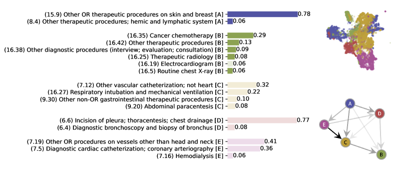
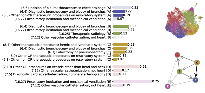
(a) Defrag on the breast cancer dataset.

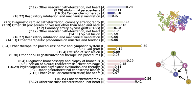
(b) Defrag on the lung cancer dataset.

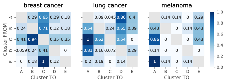
(c) Defrag on the melanoma dataset.

(d) The raw adjacency matrices.

Figure 4: Results from the MIMIC-IV experiments. Figures 4(d)-4(d): Left, TF-IDF-weighted procedure events (non-faded/most relevant, faded/least relevant); Top right: UMAP event embeddings; Lower right: Inferred pathway $G_{\to}$ (less frequent edges appear more faded). Figure 4(d): The raw adjacency matrices of $G_{\leftrightarrow}$ (normalised by the strongest edge weight) for each MIMIC-IV experiment. The y-axis indicates the source cluster, and the x-axis the destination cluster.

Figure 4 depicts the results. We start by analysing the unidirectional graph $G_{\to}$ and the treatment event distributions of each treatment cluster, as shown in Figures 4(d)-4(d). For each cancer type, Defrag identifies modality-specific treatment procedure clusters. For example, it detects cancer-related surgical procedures (clusters: “A” (breast), “C” (lung), and “C” (melanoma)) and adjuvant radio/chemotherapy procedures (clusters: “B” (breast), “B” (lung), and “A” and “E” (melanoma)), which align with ESMO best-practice guidelines [5, 41, 29]. It also uncovers cancer-related diagnostic (non-treatment) procedures and unrelated (non-cancer) clusters. We attribute the unrelated clusters to non-cancer or ICU-related treatments and disease-agnostic procedures such as catheterisation or mechanical ventilation.

Due to limitations of the MIMIC-IV dataset, we expect Defrag to find non-cancer related clusters, as a patient’s cancer diagnosis might not be their primary hospital admission reason. Defrag reliably identifies these clusters as: “C, D, E” (breast), “D, E” (lung), “B, D” (melanoma).

The summary in Figures 4(d)-4(d) depict the simpler unidirectional graph $G_{\to}$ for simplicity; however, bidirectional edges in $G_{\leftrightarrow}$ are also important for observing the relative proportions of adjuvant (after surgery) and neoadjuvant (before surgery) therapies. Figure 4(d) depicts raw adjacency matrices of $G_{\leftrightarrow}$ to emphasise these therapy proportions. In breast cancer, adjuvant (clusters “A” $\to$ “B”) and neoadjuvant (“B” $\to$ “A”) chemotherapy and radiotherapy are equally frequent. For lung cancer, adjuvant (“C” $\to$ “B”) was more common than neoadjuvant (“B” $\to$ “C”) radiotherapy. Finally, for melanoma, adjuvant chemotherapy (clusters “C” $\to$ “E”) was frequently observed, while neoadjuvant chemotherapy (“E” $\to$ “C”) was not detected at all.

Based on these results, we conclude that Defrag can identify clinically meaningful treatment pathways in AHRs. We also note that the inferred pathways are not necessarily the same as the clinical pathways, as the inferred pathways are based on the data, while the clinical pathways are based on expert knowledge. Nonetheless, elements of the inferred pathways investigated in this paper align with best-practice clinical pathways in that they identified the same treatment modalities and their relative temporal ordering (e.g., adjuvant and neoadjuvant chemotherapy in breast and lung cancer, but adjuvant chemotherapy only for melanoma). Furthermore, the inferred pathways also identified the relative proportions of adjuvant and neoadjuvant therapies for each disease within the population analysed, which can provide important insights into the treatment patterns of cancer patients.

4.2 Testing and Validation Experiments

This section tests Defrag and other pathway inference techniques on AHRs with known ground-truth pathways, as described in Section 3.2. We first run two demonstration experiments to establish the task, then conduct numerous experiments to assess the sensitivity of AHR-generation variables and evaluate Defrag’s performance against other methods.

4.2.1 Demonstration Experiments

We run two experiments that differ only in pathway size: $6$ or $12$ vertices. We use a single multinomial AHR variable with fixed support $|X|=100$ and $a=3$. The Barabási–Albert algorithm generates pathways with parameters $m=1$, $n=50$, $p=0.1$, $q=0$, $p_{i,adv}=0.6$, and for $1000$ patients. Defrag is trained with $d=64$, $16$ attention heads, $4$ encoder and decoder layers each, a feedforward dimension of $64$, and dropout of $0.2$. We train the models for $30k$ steps with a batch size of $64$ and optimised using AdamW [27] with learning rate of $10^{-4}$. The encodings are clustered with HDBSCAN [28]. We also binarise the inferred pathway edges using a threshold of $0.2$. These parameters were determined through extensive empirical experiments to balance model complexity and computational efficiency.

Figure 5 presents the results. Defrag’s inferred graph for the $6$-vertex experiment is isomorphic to the ground-truth graph, while in the $12$-vertex experiment, one vertex is disconnected, leading to incomplete inference. We quantify the performance using the adjusted mutual information score (AMI) [43], graph edit distance (GED) [38], and Weisfeiler-Lehman graph kernel (WLGK) [40]. The AMI results are $0.79$ and $0.82$, GED results are $0$ and $1$, and WLGK of $1$ and $0.93$ for the $6$- and $12$-vertex experiments, respectively. Note, it is critical to consider both AMI and GED/WLGK scores when evaluating pathway inference methods, since AMI measures semantic alignment of inferred treatments, while GED and WLGK measure the structural alignment of the inferred and ground-truth pathways. Also, in the remainder of the paper, we report GED-norm, which is the GED score normalised by the number of nodes in the ground-truth graph, enabling fair comparisons across varying graph sizes.

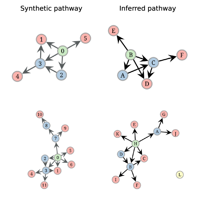
Figure 5: Results of two demonstration experiments with varying pathway sizes. Top row: $6$-vertex experiment; bottom row: $12$-vertex experiment. Left: synthetic, ground-truth pathway. Right: inferred pathway.

4.2.2 Benchmarking and Evaluation

We vary four variables across $192$ experiments to test Defrag’s performance in different circumstances: the number of vertices in the graph (${3,5,7,9}$) to adjust the pathway complexity, the size of the fixed support ($|X|:{100,1000}$) to vary the vocabulary size, the exponent $a$ of the $\mathrm{Zipf}$ variable (${1.5,2,3,4}$) to control the noisiness of events, and the number of variables (${1,2}$) to vary the amount of information available for each event observation. For each permutation of these variables, we run three experiments with different seeds, and test Defrag against several baselines (HMM, LDA, PCA, Non-negative matrix factorisation (NNMF), and Word2Vec (W2V)). For the methods that generate vectors (PCA and W2V), we cluster the vectors with hierarchical clustering to discretise the results. We also report a random baseline that randomly assigns treatments to each event.

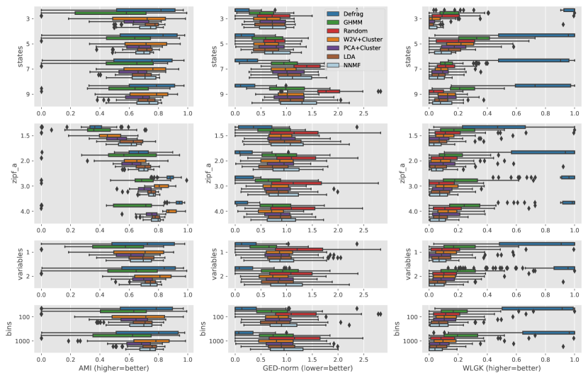
Figure 6: Results of 192 pathway inference experiments comparing Defrag to baselines. AMI (left), GED-norm (middle), and WLGK (right). The rows marginalise data synthesis variables to show how pathway inference is affected.

Table 2: Pathway inference performance of Defrag and other baselines. The mean and standard deviation (in parentheses) of the metrics are reported.

Method	AMI	GED-norm	WLGK
Defrag	$0.70$ ($0.26$)	$0.14$ ($0.28$)	$0.80$ ($0.29$)
GHMM	$0.56$ ($0.24$)	$0.75$ ($0.32$)	$0.20$ ($0.15$)
W2V+Cluster	$0.70$ ($0.19$)	$0.78$ ($0.25$)	$0.12$ ($0.11$)
PCA+Cluster	$0.64$ ($0.12$)	$0.88$ ($0.26$)	$0.09$ ($0.10$)
LDA	$0.70$ ($0.10$)	$0.86$ ($0.27$)	$0.08$ ($0.10$)
NNMF	$0.70$ ($0.09$)	$0.97$ ($0.30$)	$0.06$ ($0.05$)
Random	$0.00$ ($0.00$)	$1.16$ ($0.59$)	$0.12$ ($0.14$)

Table 2 demonstrates Defrag‘s superior ability to infer the structure of the graph, as indicated by the statistically significant improvements in GED-norm and WLGK scores. Figure 6 further explores synthetic data variables’ effects on pathway inference. Results suggest that Defrag performs better with less noisy AHR variables (higher $a$), smaller graphs, more AHR variables, and simpler vocabularies (lower $|X|$).

5 Discussion and Limitations

The pathway inference method introduced in this paper can be used by researchers and clinicians to undertake retrospective analysis of treatment pathways in AHRs. This can be used to identify common pathways and their temporal ordering, as well as to identify the relative frequencies of different pathways and their components across different patient cohorts. However, major gaps remain such as documenting and quantifying the difference between the inferred pathways and the clinical pathways that are based on expert knowledge, and cataloguing the correspondence between observed AHR events and clinically-defined treatment regimens. This is an important area for future research.

We did not explore using pre-trained features (e.g., Med2Vec [7]) – exploring the utility of such features for pathway inference is an imporant area of future work. While we show that Defrag with STLO (Tables 2 and 3) is the most effective method for pathway inference, exploring even more successful approaches is another important area of future work, one which is now enabled thanks to the synthetic data benchmarks and testing and validation framework introduced in this paper.

We reiterate that the most suitable clustering method depends on the dataset and the shape and density of encoded events. We find hierarchical methods effective across our synthetic experiments (likely due to the Barabási–Albert model) and MIMIC experiments, but centroid-based methods may be better for other datasets. Furthermore, since cluster optimisation and graph interpretability are not always correlated, future work should explore other methods of utilising the learned event vectors to enhance pathway inference.

We focus on population-level treatment pathways, but identifying rarer pathways is also essential. While Defrag can be used for this, discerning weakly-weighted edges in $G$ is challenging. Edge weights indicate frequency, not significance; thus, rarer fragments may be overlooked or undetected, as shown in Figure 5. Future work should explore methods for identifying rare but important edges in $G$.

While this study focuses on addressing the major gaps in pathway inference research (sequence modelling and evaluation), a comparitive analysis of the network inference method used in combination with Defrag’s NN is an important area for future research.

Lastly, care should be taken when interpreting the edge weights in $G_{\to}$. These weights signify the relative directional strength of edges, whereas the edge weights in bidirectional $G_{\leftrightarrow}$ signify the relative frequency of edges. $G_{\to}$ offers a high-level summary, while $G_{\leftrightarrow}$ facilitates detailed cluster transition analysis. Thus, $G_{\to}$ should be analysed alongside $G_{\leftrightarrow}$ for a comprehensive view of edge behaviour.

6 Conclusion

This study presents Defrag, an end-to-end, neural network-based method for inferring treatment pathways in administrative healthcare records (AHR). We test Defrag on several AHR datasets, demonstrating its effectiveness in identifying pathway fragments for various cancer treatments and reconstructing pathways using synthetic data. We open-source our method and synthetic data benchmarks to advance clinical pathway inference research.

Future research should focus on interpreting inferred graphs and closing the semantic gap between computationally-inferred and clinically-derived pathways. Future pathway inference research should iterate on and compare to Defrag, utilising established benchmarks in the testing and validation framework. Additionally, examining anomalies in inferred pathways can help to inform clinical pathway development.

CRediT authorship contribution statement

A. Wilkins-Caruana: Conceptualisation, methodology, software, validation, formal analysis, investigation, resources, data curation, writing - original draft, visualisation.

M. Bandara, K. Musial: Writing - review and editing, supervision.

D. Catchpoole, P. J. Kennedy: Writing - review and editing, supervision, project administration, funding acquisition.

Declaration of Competing Interest

The authors declare that they have no known competing financial interests or personal relationships that could have appeared to influence the work reported in this paper.

Appendix A Windowed-Attention

The window size $w$ of the attention mask in the Transformer encoder controls the amount of temporal context for the learned semantic-temporal encodings. Figure 7 shows how the value of $w$ can result in three kinds of learned embedding behaviour. Unlike Figure 4, we omit the TF-IDF-weighted cluster event distributions; these histograms relay semantic meaning, which remains largely unchanged as $w$ varies. Instead, Figure 7 focuses on showing how the temporal meaning of clusters changes as $w$ varies. This is shown via the distribution of encoded events $X_{\mathbf{enc}}$ in Figure 7(b), and the number of cluster transitions in each inferred graph in Figure 7(b), which is given as $\sum_{p\in V}\sum_{q\in V}w_{p,q,p\neq q}$ as per Equation 6.

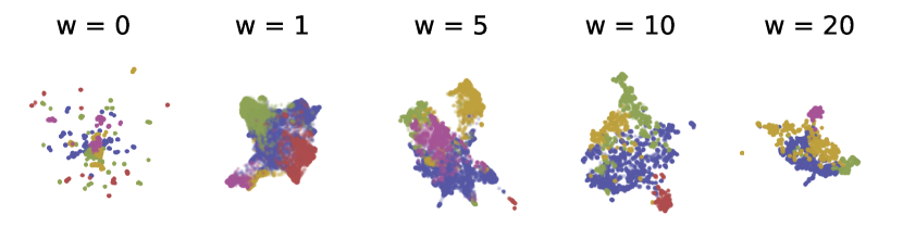
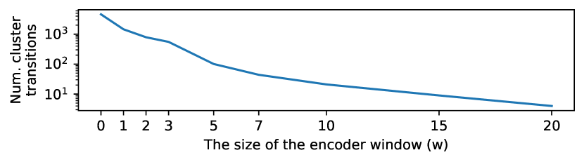
(a) UMAP embedding of $X_{\mathbf{enc}}$ on the breast cancer dataset for different values of $w$ in the windowed-attention.

(b) The number of cluster transitions on the breast cancer dataset for different values of $w$ in the windowed-attention.

Figure 7: This figure uses the breast cancer dataset to show how the behaviour of the learned semantic-temporal encoded event representations (top row) and the number of event-level cluster transitions in the inferred graph vary as the size $w$ of the encoder window varies.

When $w=0$ events can not attend to each other, and thus the learned representations are semantic only (i.e., no temporal information is used), with the representation space containing many regions of high-density. The space must represent a total of $|X|$ possible discrete events.

When $w=1$, each event can attend to both of its neighbours from the sequence, and thus temporal information is utilised which results in a smoother representation space. If we assume that $f_{\mathbf{enc}}$ is not permutation invariant (which is a good approximation when $w$ is small), then the upper bound of unique neighbourhoods ($|X|!/(|X|-(2w+1))!$ or $|X|!/(|X|-3)!$) is significantly larger than the number of events ($|X|$). This has the effect of increasing the utilisation of the representation space, as indicated by the more uniform UMAP embedding. However, since some adjacent events may appear together quite often and thus have similar semantic-temporal representations, the number of cluster transitions between adjacent events decreases.

As $w$ increases further, the neighbourhoods of adjacent events begin to contain a greater proportion of redundant information. For example, if $w=5$, then the neighbourhoods of two adjacent events would contain the same sequence of 10 events, a sequence which becomes increasingly unlikely to belong to more than one patient. This redundancy is an intentional consequence of the relative positional encoding [39] used in the Transformer’s attention, which is required to make $f_{\mathbf{enc}}$ consider the sequence ordering. That is, relative positional encoding makes $f_{\mathbf{enc}}$ translation-invariant. This would not be the case with absolute positional encoding, (as in [42]) which would see the number of event-neighbourhood permutations increase significantly and make the representation space highly inefficient. Thus, as $w$ increases, the representation of individual events emphasises less of the information about any one specific event and more of the information about one specific patient. This all has the effect of making the representation space less smooth, while continuing to reduce the number of cluster transitions between adjacent events.

In practice, the choice of $w$ will depend on the granularity of the AHR dataset used. We found that inferred graphs were quite similar for $1\leq w\leq 5$. As $w$ becomes too large, there is not enough information to infer a graph with sufficient detail for interpretation.

Appendix B Relative Positional Encoding

Figure 8 shows UMAP embeddings of the breast cancer experiment, each run with different positional encoding schemes. While the experiment that used relative positional encoding successfully separates three treatment modalities shown, the absolute positional encoding and no positional encoding experiments do not separate the modalities well at all. Separation of different treatment modalities is critical for generating semantic-temporal representations that are useful for pathway inference.

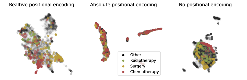
Figure 8: UMAP embeddings for the breast cancer experiment, with relative positional encoding (left), absolute positional encoding (middle), and no positional encoding at all (right). The colours depict events from three breast cancer treatment modalities.

Appendix C STLO Discussion

C.1 Comparison with other self-supervised objectives

We provide pathway inference results for the STLO and other self-supervised objectives in Table 3. Results are reported on the 192 synthetic datasets from Section 4.2.2.

The results indicate that the STLO is the best self-supervised objective for pathway inference. Notably, the next-best objective, SimCSE, is competitive with the STLO in terms of pathway inference ability (GED-norm and WLGK), but its ability to infer semantically accurate clusters is significantly worse (AMI). This demonstrates that the STLO has a unique ability to learn both semantically and temporally meaningful representations of treatments.

Table 3: Pathway inference performance of Defrag when trained with various self-supervised learning objectives. The mean and standard deviation (in parentheses) of the metrics are reported.

Method	AMI	GED-norm	WLGK
Defrag + STLO	$0.70$ ($0.26$)	$0.14$ ($0.28$)	$0.80$ ($0.29$)
Defrag + SimCSE	$0.59$ ($0.23$)	$0.18$ ($0.27$)	$0.74$ ($0.31$)
Defrag + MSE	$0.50$ ($0.27$)	$0.29$ ($0.36$)	$0.66$ ($0.35$)
Defrag + Barlow	$0.48$ ($0.24$)	$0.36$ ($0.43$)	$0.57$ ($0.37$)
Random	$0.00$ ($0.00$)	$1.16$ ($0.59$)	$0.12$ ($0.14$)

Furthermore, Figure 9 depicts the TF-IDF-weighted cluster distributions of the breast cancer experiment, each trained with a different loss function. The information entropy of the STLO-based clusters is 0.9, 2.0, 1.8, 0.9, 1.4 nats (mean: 1.4) while the information entropy of the reconstruction-based clusters is 2.1, 2.2, 2.1, 1.9, 2.1 nats (mean: 2.1). Not only is the information entropy of the STLO-based experiment significantly lower than the same experiment trained with an auto-encoding reconstruction objective on the decoder — indicating that the clusters are not grouping temporally- and semantically-similar treatments — the histograms also show that modality-specific treatments (e.g., “Other OR therapeutic procedures on skin and breast”) are isolated in the STLO-based experiment, but are present in many different clusters in the reconstruction-based experiment.

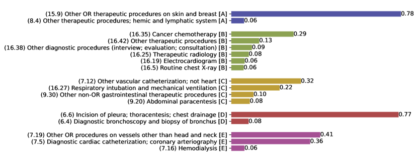
(a) Breast cancer experiment trained with STLO.

(b) Breast cancer experiment trained with an auto-encoding reconstruction objective on the decoder (mean squared error).

Figure 9: TF-IDF-weighted distributions of treatment codes in the breast cancer experiment.

C.2 Two-Treatment Assumption

One inductive bias of the STLO is that it assumes that there are only two treatments in the sequence. This is a pragmatic choice that is made to simplify the training process since it is not possible to know how many treatments there shall be since each patient is different and the data contains no such treatment annotations. Furthermore, it is not practical to determine how many treatments there are in the sequence in an instantaneous, dynamic way during training. . While this choice is not ideal, it is not a significant limitation of the STLO for the specific purpose of learning semantic and temporal information about treatments. Thus, we make the pragmatic choice to pick a static value (two) and pursue several strategies to mitigate the consequences of this decision, which we enumerate below.

1. We train with short patient subsequences rather than entire patient sequences since shorter subsequences are more likely to contain a small number of treatments.

2. The STLO’s two-treatment assumption is not a hard requirement. For example, should the short training subsequence contain three treatments instead of two, then the STLO will group two of the contiguous treatments together, and, to make the least bad decision about which treatments to merge, the model must use its knowledge of the semantic and temporal information of these treatments, which further contributes to the overall objective of learning semantic and temporal treatment information.

3. The ‘treatment’ concept is abstract, not concrete. The STLO loss function is perhaps better conceptualised simply as a contrastive objective – i.e., given a sequence of events, determine the point within the sequence that separates the events into two contiguous groups such that their within-group semantic and temporal similarity is maximised. Furthermore, this abstraction goes beyond the model, since the definition of a ‘treatment’ varies across medical disciplines and data formats. For example, patients will likely receive fewer treatments in a emergency department visit, and more treatments across the course of a cancer treatment.

4. Finally, while the STLO loss at the decoder backpropagates through the encoder during training, it is not the only backpropagation path since the encoder and decoder paths diverge in the network architecture. We refer to [42] for a detailed description of the Transformer architecture. Therefore, the unique paths introduce the opportunity for the encoder and decoder to learn independent features that are relevant to the decoder’s objective. Finally, we reiterate that the encoder’s representations are intermediate in the Transformer and that intermediate features do not need to adhere to the training objective, rather they contribute useful information towards this goal.

C.3 Encoder-decoder setup

We choose the encoder-decoder setup of the Transformer (as opposed to a decoder-only setup) since it allows us to decouple where STLO is applied in the network from where the pathway inference is performed. This is important since STLO is computed on the decoder, but the pathway inference is conducted using the encoder’s representations. Figure 10 shows that the encoder’s naturally clusters the data in alignment with the ground-truth annotations, which demonstrates that the proposed neural network configuration is fit for purpose.

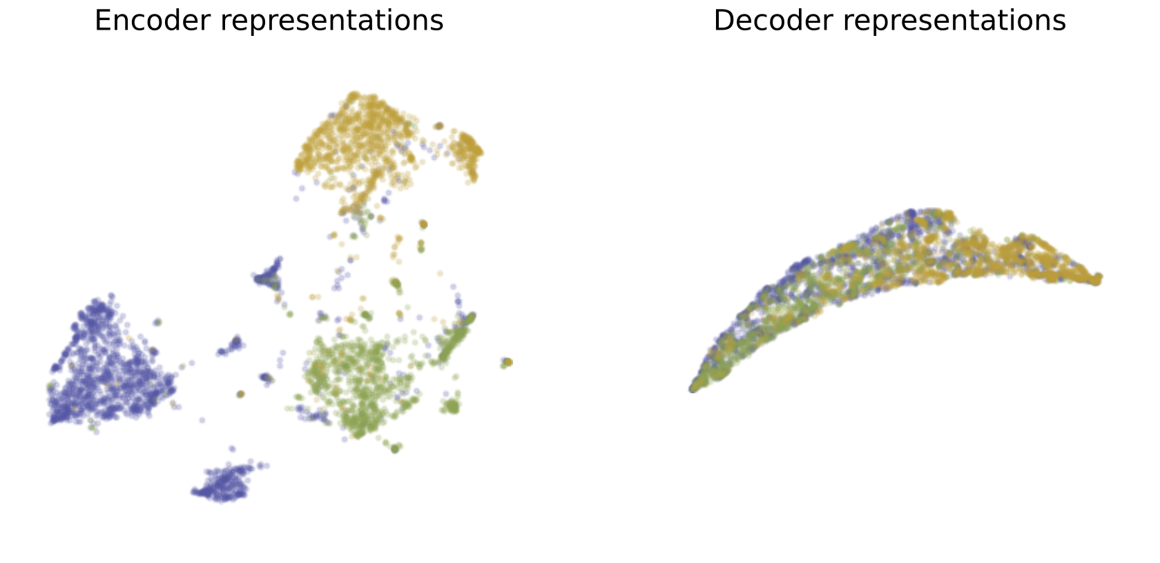
Figure 10: Empirical evidence from a synthetic data experiment containing three distinct treatments. The topology of the generated event representations suggests that clusters in the encoder’s representations naturally align with ground-truth annotations.

Appendix D Cluster Optimisation

In the synthetic data experiments, optimal clustering on encoded events is determined using a grid search, selecting the parameters for the clustering method that optimises an unsupervised metric. No significant practical differences were found among the following metrics: Calinski-Harabasz [4], silhouette [37], and Davies-Bouldin scores [9]. Figure 11 depicts each of the grid-search scores for all experiments in Section 4.2.2. All unsupervised scores roughly correlate with the supervised AMI [43].

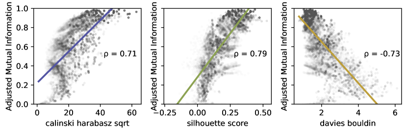
Figure 11: The correlation of unsupervised clustering metrics with AMI is examined. The square root of Calinski-Harabasz is plotted due to its quadratic scaling behaviour.

While automating the selection of clustering parameters was useful for systematic experiments, this approach was not as useful for experiments on MIMIC-IV data. This is because optimal clustering parameters depend on the inductive biases of the metric and model, and are not necessarily correlated with which partition over $X_{\mathbf{enc}}$ yields the most interpretable treatment clusters and inferred pathway $G$. For this reason, we chose to use identical clustering parameters across all MIMIC-IV experiments to minimise the role of parameter selection in influencing our analysis of the results.

In practice, an analysis should carefully examine several clustering algorithms and clustering parameters (i.e., number and shape of clusters) to inform a comprehensive analysis of treatment clusters. For the MIMIC-IV experiments in Section 4.1, we chose to infer 5 clusters for the following reasons: 1) to be consistent across each of the three experiments, 2) five clusters was the minimum needed to infer sufficient granularity of the inferred pathway clusters, 3) inferred pathways containing more than five clusters become increasingly difficult to interpret, and 4) When inferring more than five clusters, we found that the encoded events were ‘over-clustered’, in that a single semantic cluster in the 5-cluster case was separated into two functionally similar clusters in cases where the number of clusters was greater than five. However, other values for the number of clusters may be more suitable for other experiments – to this end, we reiterate that inferring more clusters yields more granular clusters, vise versa.

Appendix E Synthetic AHR Plausibility

Figure 12 compares the distribution of synthetically generated AHR events with the ICD9 procedure codes in the MIMIC-IV breast cancer dataset. Synthetic distributions are more aligned when generated with more code variance (lower $a$) and larger graphs. However, in general, the synthetic data can align or diverge with real AHR datasets depending on the data generation parameters. Alignment and divergence are both desirable properties of such a testing and validation framework, since the goal is to simulate different kinds of AHRs, not align too closely to any specific dataset.

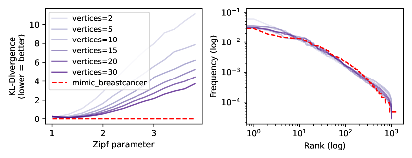
Figure 12: Left: KL-Divergence between synthetic data and MIMIC-IV distributions as the number of vertices in $G$ and Zipf parameter $a$ vary. Right: Rank-frequency distribution of the closest synthesised datasets for different-sized graphs and the MIMIC-IV distribution.

References

- Aalst [2012] Aalst, W.V.D., 2012. Process mining. Communications of the ACM 55, 76–83. URL: https://doi.org/10.1145%2F2240236.2240257, doi:10.1145/2240236.2240257.
- Albert and Barabási [2000] Albert, R., Barabási, A.L., 2000. Topology of evolving networks: local events and universality. Physical review letters 85, 5234.
- Baker et al. [2017] Baker, K., Dunwoodie, E., Jones, R.G., Newsham, A., Johnson, O., Price, C.P., Wolstenholme, J., Leal, J., McGinley, P., Twelves, C., Hall, G., 2017. Process mining routinely collected electronic health records to define real-life clinical pathways during chemotherapy. International Journal of Medical Informatics 103, 32–41. URL: https://doi.org/10.1016%2Fj.ijmedinf.2017.03.011, doi:10.1016/j.ijmedinf.2017.03.011.
- Calinski and Harabasz [1974] Calinski, T., Harabasz, J., 1974. A dendrite method for cluster analysis. Communications in Statistics - Theory and Methods 3, 1–27. URL: https://doi.org/10.1080%2F03610927408827101, doi:10.1080/03610927408827101.
- Cardoso et al. [2019] Cardoso, F., Kyriakides, S., Ohno, S., Penault-Llorca, F., Poortmans, P., Rubio, I., Zackrisson, S., Senkus, E., 2019. Early breast cancer: ESMO clinical practice guidelines for diagnosis, treatment and follow-up. Annals of Oncology 30, 1194–1220. URL: https://doi.org/10.1093%2Fannonc%2Fmdz173, doi:10.1093/annonc/mdz173.
- Chen et al. [2017] Chen, J., Wei, W., Guo, C., Tang, L., Sun, L., 2017. Textual analysis and visualization of research trends in data mining for electronic health records. Health Policy and Technology 6, 389–400. URL: https://doi.org/10.1016%2Fj.hlpt.2017.10.003, doi:10.1016/j.hlpt.2017.10.003.
- Choi et al. [2016] Choi, E., Bahadori, M.T., Searles, E., Coffey, C., Thompson, M., Bost, J., Tejedor-Sojo, J., Sun, J., 2016. Multi-layer representation learning for medical concepts, ACM. URL: https://doi.org/10.1145%2F2939672.2939823, doi:10.1145/2939672.2939823.
- Choi et al. [2018] Choi, E., Xiao, C., Stewart, W.F., Sun, J., 2018. Mime: Multilevel medical embedding of electronic health records for predictive healthcare, in: 32nd Conference on Neural Information Processing Systems, NeurIPS 2018, pp. 4547–4557.
- Davies and Bouldin [1979] Davies, D.L., Bouldin, D.W., 1979. A cluster separation measure. IEEE Transactions on Pattern Analysis and Machine Intelligence PAMI-1, 224–227. URL: https://doi.org/10.1109%2Ftpami.1979.4766909, doi:10.1109/tpami.1979.4766909.
- De Weerdt et al. [2013] De Weerdt, J., Caron, F., Vanthienen, J., Baesens, B., 2013. Getting a grasp on clinical pathway data: An approach based on process mining, in: Washio, T., Luo, J. (Eds.), Emerging Trends in Knowledge Discovery and Data Mining. Springer Berlin Heidelberg, Berlin, Heidelberg, pp. 22–35. doi:10.1007/978-3-642-36778-6_3.
- DiMatteo [2004] DiMatteo, M.R., 2004. Variations in patients’ adherence to medical recommendations. Medical Care 42, 200–209. URL: https://doi.org/10.1097%2F01.mlr.0000114908.90348.f9, doi:10.1097/01.mlr.0000114908.90348.f9.
- Ebben et al. [2013] Ebben, R.H., Vloet, L.C., Verhofstad, M.H., Meijer, S., de Groot, J.A.M., van Achterberg, T., 2013. Adherence to guidelines and protocols in the prehospital and emergency care setting: a systematic review. Scandinavian Journal of Trauma, Resuscitation and Emergency Medicine 21. URL: https://doi.org/10.1186%2F1757-7241-21-9, doi:10.1186/1757-7241-21-9.
- Fauman [2007] Fauman, M., 2007. How do physicians use practice guidelines? Drug Benefit Trends 19, 237.
- Gao et al. [2021] Gao, T., Yao, X., Chen, D., 2021. Simcse: Simple contrastive learning of sentence embeddings. arXiv preprint arXiv:2104.08821 .
- Ghahramini [2001] Ghahramini, Z., 2001. An introduction to hidden markov models and bayesian networks, in: Series in Machine Perception and Artificial Intelligence. World Scientific, pp. 9–41. URL: https://doi.org/10.1142%2F9789812797605_0002, doi:10.1142/9789812797605_0002.
- Goncalves et al. [2020] Goncalves, A., Ray, P., Soper, B., Stevens, J., Coyle, L., Sales, A.P., 2020. Generation and evaluation of synthetic patient data. BMC Medical Research Methodology 20. URL: https://doi.org/10.1186%2Fs12874-020-00977-1, doi:10.1186/s12874-020-00977-1.
- Guzzo et al. [2021] Guzzo, A., Rullo, A., Vocaturo, E., 2021. Process mining applications in the healthcare domain: A comprehensive review. WIREs Data Mining and Knowledge Discovery 12. URL: https://doi.org/10.1002%2Fwidm.1442, doi:10.1002/widm.1442.
- Huang et al. [2018a] Huang, C.Z.A., Vaswani, A., Uszkoreit, J., Shazeer, N., Simon, I., Hawthorne, C., Dai, A.M., Hoffman, M.D., Dinculescu, M., Eck, D., 2018a. Music transformer. arXiv preprint URL: https://arxiv.org/abs/1809.04281, arXiv:1809.04281.
- Huang et al. [2014] Huang, Z., Dong, W., Ji, L., Gan, C., Lu, X., Duan, H., 2014. Discovery of clinical pathway patterns from event logs using probabilistic topic models. Journal of Biomedical Informatics 47, 39--57. URL: https://doi.org/10.1016%2Fj.jbi.2013.09.003, doi:10.1016/j.jbi.2013.09.003.
- Huang et al. [2018b] Huang, Z., Ge, Z., Dong, W., He, K., Duan, H., 2018b. Probabilistic modeling personalized treatment pathways using electronic health records. Journal of Biomedical Informatics 86, 33--48. URL: https://doi.org/10.1016%2Fj.jbi.2018.08.004, doi:10.1016/j.jbi.2018.08.004.
- Huang et al. [2013] Huang, Z., Lu, X., Duan, H., 2013. Latent treatment pattern discovery for clinical processes. Journal of Medical Systems 37. URL: https://doi.org/10.1007%2Fs10916-012-9915-2, doi:10.1007/s10916-012-9915-2.
- Johnson et al. [2020] Johnson, A., Bulgarelli, L., Pollard, T., Horng, S., Celi, L.A., Mark IV, R., 2020. Mimic-iv (version 0.4). PhysioNet .
- Lang et al. [2008] Lang, M., B"urkle, T., Laumann, S., Prokosch, H.U., 2008. Process mining for clinical workflows: challenges and current limitations, in: EHealth beyond the horizon: get it there: proceedings of MIE2008 the XXIst international congress of the european federation for medical informatics, p. 229.
- Lim et al. [2021] Lim, J., Kim, K., Cho, M., Baek, H., Kim, S., Hwang, H., Yoo, S., Song, M., 2021. Deriving a sophisticated clinical pathway based on patient conditions from electronic health record data, in: Leemans, S., Leopold, H. (Eds.), Lecture Notes in Business Information Processing. Springer International Publishing, pp. 356--367. URL: https://doi.org/10.1007%2F978-3-030-72693-5_27, doi:10.1007/978-3-030-72693-5_27.
- Lim et al. [2022] Lim, J., Kim, K., Song, M., Yoo, S., Baek, H., Kim, S., Park, S., Jeong, W.J., 2022. Assessment of the feasibility of developing a clinical pathway using a clinical order log. Journal of Biomedical Informatics 128, 104038. URL: https://doi.org/10.1016%2Fj.jbi.2022.104038, doi:10.1016/j.jbi.2022.104038.
- Litchfield et al. [2018] Litchfield, I., Hoye, C., Shukla, D., Backman, R., Turner, A., Lee, M., Weber, P., 2018. Can process mining automatically describe care pathways of patients with long-term conditions in UK primary care? a study protocol. BMJ Open 8, e019947. URL: https://doi.org/10.1136%2Fbmjopen-2017-019947, doi:10.1136/bmjopen-2017-019947.
- Loshchilov and Hutter [2019] Loshchilov, I., Hutter, F., 2019. Decoupled weight decay regularization. arXiv preprint URL: https://arxiv.org/abs/1711.05101, arXiv:1711.05101.
- McInnes et al. [2017] McInnes, L., Healy, J., Astels, S., 2017. HDBSCAN: Hierarchical density based clustering. The Open Journal 2, 205. URL: https://doi.org/10.21105/joss.00205, doi:10.21105/joss.00205.
- Michielin et al. [2019] Michielin, O., van Akkooi, A., Ascierto, P., Dummer, R., Keilholz, U., 2019. Cutaneous melanoma: ESMO clinical practice guidelines for diagnosis, treatment and follow-up. Annals of Oncology 30, 1884--1901. URL: https://doi.org/10.1093%2Fannonc%2Fmdz411, doi:10.1093/annonc/mdz411.
- Mikolov et al. [2013] Mikolov, T., Sutskever, I., Chen, K., Corrado, G.S., Dean, J., 2013. Distributed representations of words and phrases and their compositionality. Advances in neural information processing systems 26.
- Oliart et al. [2022] Oliart, E., Rojas, E., Capurro, D., 2022. Are we ready for conformance checking in healthcare? measuring adherence to clinical guidelines: A scoping systematic literature review. Journal of Biomedical Informatics 130, 104076. URL: https://doi.org/10.1016%2Fj.jbi.2022.104076, doi:10.1016/j.jbi.2022.104076.
- Panella [2003] Panella, M., 2003. Reducing clinical variations with clinical pathways: do pathways work? International Journal for Quality in Health Care 15, 509--521. URL: https://doi.org/10.1093%2Fintqhc%2Fmzg057, doi:10.1093/intqhc/mzg057.
- Piantadosi [2014] Piantadosi, S.T., 2014. Zipf’s word frequency law in natural language: A critical review and future directions. Psychonomic Bulletin & Review 21, 1112--1130. URL: https://doi.org/10.3758%2Fs13423-014-0585-6, doi:10.3758/s13423-014-0585-6.
- Rebuge and Ferreira [2012] Rebuge, Á., Ferreira, D.R., 2012. Business process analysis in healthcare environments: A methodology based on process mining. Information Systems 37, 99--116. URL: https://doi.org/10.1016%2Fj.is.2011.01.003, doi:10.1016/j.is.2011.01.003.
- Rotter et al. [2011] Rotter, T., Kinsman, L., James, E., Machotta, A., Willis, J., Snow, P., Kugler, J., 2011. The effects of clinical pathways on professional practice, patient outcomes, length of stay, and hospital costs. Evaluation & the Health Professions 35, 3--27. URL: https://doi.org/10.1177%2F0163278711407313, doi:10.1177/0163278711407313.
- Rotter et al. [2010] Rotter, T., Kinsman, L., James, E.L., Machotta, A., Gothe, H., Willis, J., Snow, P., Kugler, J., 2010. Clinical pathways: effects on professional practice, patient outcomes, length of stay and hospital costs. Cochrane Database of Systematic Reviews URL: https://doi.org/10.1002%2F14651858.cd006632.pub2, doi:10.1002/14651858.cd006632.pub2.
- Rousseeuw [1987] Rousseeuw, P.J., 1987. Silhouettes: A graphical aid to the interpretation and validation of cluster analysis. Journal of Computational and Applied Mathematics 20, 53--65. URL: https://doi.org/10.1016%2F0377-0427%2887%2990125-7, doi:10.1016/0377-0427(87)90125-7.
- Sanfeliu and Fu [1983] Sanfeliu, A., Fu, K.S., 1983. A distance measure between attributed relational graphs for pattern recognition. IEEE Transactions on Systems, Man, and Cybernetics SMC-13, 353--362. URL: https://doi.org/10.1109%2Ftsmc.1983.6313167, doi:10.1109/tsmc.1983.6313167.
- Shaw et al. [2018] Shaw, P., Uszkoreit, J., Vaswani, A., 2018. Self-attention with relative position representations. arXiv preprint URL: https://arxiv.org/abs/1803.02155, arXiv:1803.02155.
- Shervashidze et al. [2011] Shervashidze, N., Schweitzer, P., Van Leeuwen, E.J., Mehlhorn, K., Borgwardt, K.M., 2011. Weisfeiler-lehman graph kernels. Journal of Machine Learning Research 12.
- Vansteenkiste et al. [2014] Vansteenkiste, J., Crinò, L., Dooms, C., Douillard, J., Faivre-Finn, C., Lim, E., Rocco, G., Senan, S., Schil, P.V., Veronesi, G., Stahel, R., Peters, S., Felip, E., Stahel, R., Felip, E., Peters, S., Kerr, K., Besse, B., Vansteenkiste, J., Eberhardt, W., Edelman, M., Mok, T., O'Byrne, K., Novello, S., Bubendorf, L., Marchetti, A., Baas, P., Reck, M., Syrigos, K., Paz-Ares, L., Smit, E.F., Meldgaard, P., Adjei, A., Nicolson, M., Crinò, L., Schil, P.V., Senan, S., Faivre-Finn, C., Rocco, G., Veronesi, G., Douillard, J.Y., Lim, E., Dooms, C., Weder, W., Ruysscher, D.D., Pechoux, C.L., Leyn, P.D., Westeel, V., 2014. 2nd ESMO consensus conference on lung cancer: early-stage non-small-cell lung cancer consensus on diagnosis, treatment and follow-up. Annals of Oncology 25, 1462--1474. URL: https://doi.org/10.1093%2Fannonc%2Fmdu089, doi:10.1093/annonc/mdu089.
- Vaswani et al. [2017] Vaswani, A., Shazeer, N., Parmar, N., Uszkoreit, J., Jones, L., Gomez, A.N., Kaiser, L., Polosukhin, I., 2017. Attention is all you need, in: Proceedings of the 31st International Conference on Neural Information Processing Systems, pp. 5998--6008.
- Vinh et al. [2009] Vinh, N.X., Epps, J., Bailey, J., 2009. Information theoretic measures for clusterings comparison, ACM Press. URL: https://doi.org/10.1145%2F1553374.1553511, doi:10.1145/1553374.1553511.
- Wilcoxon [1945] Wilcoxon, F., 1945. Individual comparisons by ranking methods. Biometrics Bulletin 1, 80. URL: https://doi.org/10.2307%2F3001968, doi:10.2307/3001968.
- Wolfram [2002] Wolfram, S., 2002. A New Kind of Science. Wolfram Media. URL: https://www.wolframscience.com.
- Xu et al. [2016] Xu, X., Jin, T., Wei, Z., Lv, C., Wang, J., 2016. TCPM: Topic-based clinical pathway mining, in: 2016 IEEE First International Conference on Connected Health: Applications, Systems and Engineering Technologies (CHASE), IEEE. URL: https://doi.org/10.1109%2Fchase.2016.17, doi:10.1109/chase.2016.17.
- Xu et al. [2017] Xu, X., Jin, T., Wei, Z., Wang, J., 2017. Incorporating topic assignment constraint and topic correlation limitation into clinical goal discovering for clinical pathway mining. Journal of Healthcare Engineering 2017, 1--13. URL: https://doi.org/10.1155%2F2017%2F5208072, doi:10.1155/2017/5208072.
- Yadav et al. [2018] Yadav, P., Steinbach, M., Kumar, V., Simon, G., 2018. Mining electronic health records (EHRs). ACM Computing Surveys 50, 1--40. URL: https://doi.org/10.1145%2F3127881, doi:10.1145/3127881.
- Yan et al. [2016] Yan, C., Chen, Y., Li, B., Liebovitz, D., Malin, B., 2016. Learning clinical workflows to identify subgroups of heart failure patients, in: AMIA Annual Symposium Proceedings, American Medical Informatics Association. p. 1248.
- Yang and Su [2014] Yang, W., Su, Q., 2014. Process mining for clinical pathway: Literature review and future directions, in: 2014 11th International Conference on Service Systems and Service Management (ICSSSM), IEEE. URL: https://doi.org/10.1109%2Ficsssm.2014.6943412, doi:10.1109/icsssm.2014.6943412.
- Yang et al. [2020] Yang, Z., Dehmer, M., Yli-Harja, O., Emmert-Streib, F., 2020. Combining deep learning with token selection for patient phenotyping from electronic health records. Scientific Reports 10. URL: https://doi.org/10.1038%2Fs41598-020-58178-1, doi:10.1038/s41598-020-58178-1.
- Yu et al. [2014] Yu, P., Artz, D., Warner, J., 2014. Electronic health records (EHRs): Supporting ASCO's vision of cancer care. American Society of Clinical Oncology Educational Book , 225--231URL: https://doi.org/10.14694%2Fedbook_am.2014.34.225, doi:10.14694/edbook_am.2014.34.225.
- Zbontar et al. [2021] Zbontar, J., Jing, L., Misra, I., LeCun, Y., Deny, S., 2021. Barlow twins: Self-supervised learning via redundancy reduction, in: International Conference on Machine Learning, PMLR. pp. 12310--12320.
- Zhang et al. [2022] Zhang, X., Zhao, Y., Yan, C., Derr, T., Chen, Y., 2022. Inferring ehr utilization workflows through audit logs, in: AMIA Annual Symposium Proceedings, American Medical Informatics Association. p. 1247.
- Zhang et al. [2015a] Zhang, Y., Padman, R., Patel, N., 2015a. Paving the COWpath: Learning and visualizing clinical pathways from electronic health record data. Journal of Biomedical Informatics 58, 186--197. URL: https://doi.org/10.1016%2Fj.jbi.2015.09.009, doi:10.1016/j.jbi.2015.09.009.
- Zhang et al. [2015b] Zhang, Y., Padman, R., Wasserman, L., Patel, N., Teredesai, P., Xie, Q., 2015b. On clinical pathway discovery from electronic health record data. IEEE Intelligent Systems 30, 70--75. URL: https://doi.org/10.1109%2Fmis.2015.14, doi:10.1109/mis.2015.14.