Constraining scotogenic dark matter and primordial black holes using
gravitational waves

Abstract

The lightest $Z_{2}$ odd particle in the scotogenic model, referred to as scotogenic dark matter (DM), is a widely studied candidate for DM. This scotogenic DM is generated through well-known thermal processes as well as via the evaporation of primordial black holes (PBHs). Recent reports suggested that the curvature fluctuations of PBHs during an epoch dominated by these entities in the early universe can serve as the source of so-called induced gravitational waves (GWs). In this study, we demonstrate that stringent constraints on the mass of scotogenic DM and PBHs can be obtained through the detection of induced GWs using future detectors.

I Introduction

The existence of dark matter (DM) and the minute scale of neutrino masses have been a longstanding mystery in cosmology and particle physics. The scotogenic model offers a unified explanation for the presence of DM and the origin of tiny neutrino masses [1]. In this model, neutrino masses are generated from one-loop interactions mediated by a DM candidate. The DM in the scotogenic model (scotogenic DM) is generated due to the thermal processes in the early universe, which has garnered extensive attention in the literature. [2, 3, 30, 4, 5, 6, 7, 8, 9, 10, 11, 12, 13, 14, 15, 16, 17, 18, 19, 20, 21, 22, 23, 24, 25, 26, 27, 28, 29, 31, 32, 33, 34, 35, 36, 37, 38, 39, 40, 41, 42, 43, 44, 45, 46, 47, 48, 49, 52, 50, 51].

The evaporation of primordial black holes (PBHs) serve as a potential source for the production of scotogenic DM [53, 54]. These PBHs are among the types of black holes formed in the early universe [55, 56, 57, 58]. PBHs emit particles via the Hawking radiation [59]. Owing to the Hawking radiation induced by gravity, PBHs are expected to produce some additional particles in addition to standard model particles, independent of their nongravitational interactions [60, 61, 62, 63, 64, 65, 66, 67, 68, 69, 70, 72, 71, 73, 74, 75, 76, 79, 80, 82, 81, 83, 77, 78]. Thus, given the coexistence of the scotogenic DM and PBHs in the universe, the scotogenic DM should be produced by thermal processes as well as PBH evaporation.

Moreover, PBHs have been identified as a potential source of DMs and gravitational waves (GWs) [84, 85, 86, 87, 88, 89, 90, 91, 92, 93, 94, 95, 96, 97]. In the last stage of the inflation, immediately after horizon reentry, the primordial fluctuations in the curvature perturbation can act as a source of induced GWs. Furthermore, the PBH formation is invariably accompanied by GWs. The induced GWs have garnered considerable research interest as they could be detected by the currently developing future GW observations such as Hanford-Livingstone-Virgo-KAGRA (HLVK, or aLIGO-aVirgo-KAGRA) [98, 99, 100, 101], Einstein Telescope (ET) [102, 103], Cosmic Explorer (CE) [104], Laser Interferometer Space Antenna (LISA) [105], Deci-Hertz Interferometer Gravitational-Wave Observatory (DECIGO) [106, 107] and Big Bang Observer (BBO) [108, 109].

Recent reports indicated that GWs could be induced by sources other than the primordial fluctuation [110]. Immediately after formation, PBHs are randomly distributed in space according to approximate Poisson statistics. Although the PBH gas behaves as pressureless dust, the spatially inhomogeneous distribution leads to isocurvature density fluctuations. At a later time, if the initial fraction of PBHs is sufficiently large, they would eventually overcome the energy density of the radiation component, thereby dominating the universe. During the transition from an early radiation-dominated epoch to a PBH-dominated (in other words, an early matter-dominated) epoch, the initial isocurvature fluctuations are transmuted into curvature perturbations, which consequently act as sources for secondary GWs [111, 110, 112, 113, 114].

In a study reported in Ref. [114], constraints on heavy particles serving as DM in the seesaw mechanism and PBHs are inferred using induced GWs in the PBH-dominated epoch. The seesaw mechanism is a widely acknowledged model for the generation of diminutive neutrino masses [115, 116, 117, 118, 119]. Currently, the seesaw mechanism and the scotogenic model represent the most extensively researched paradigms for neutrino mass production.

In this study, we postulate that scotogenic DM constitutes the DM and that a PBH-dominated epoch was existent in the early universe. By employing a methodology analogous to that reported in Ref.[114], we estimate the constraints on the masses of scotogenic DM and PBHs based on induced GWs. Although Ref. [114] suggests DM production only through PBH evaporation, this study additionally incorporates the freeze-out mechanism for scotogenic DM production. We demonstrate that future GW detectors could impose rigorous constraints on the masses of scotogenic DM and PBHs.

The remainder of this article is organized as follows. In Sec. II, we offer a short review of scotogenic DM and PBHs, emphasizing DM production via the freeze-out mechanism and PBH evaporation, which is one of the primary topics. In addition, we focus on the necessary condition of the initial density of PBHs to establish a PBH-dominated epoch and maintain consistency with Big Bang Nucleosynthesis (BBN). In Sec. III, we present the stringent constraints on the mass of scotogenic DM and PBHs deduced from induced GWs. The article concludes with a summary of the key findings in Sec. IV.

II Scotogenic dark matter and primordial black holes

II.1 Scotogenic model

In the scotogenic model, three new Majorana $SU(2)_{L}$ singlets $N_{k}$ $(k=1,2,3)$ with mass $M_{k}$ and one new scalar $SU(2)_{L}$ doublet $(\eta^{+},\eta^{0})$ are introduced into the standard model [1]. The Lagrangian and scalar potential relevant for this study are expressed as

$$\mathcal{L} = Y_{\alpha k}(\bar{\nu}_{\alpha L}\eta^{0}-\bar{\ell}_{\alpha L}\eta^{+})N_{k}+\frac{1}{2}M_{k}\bar{N}_{k}N^{C}_{k}+h.c.,$$

$$V = \frac{1}{2}\lambda(\phi^{\dagger}\eta)^{2}+h.c.,$$ (1)

where $L_{\alpha}=(\nu_{\alpha},\ell_{\alpha})$ $(\alpha=e,\mu,\tau)$ denotes the left-handed lepton doublet and $\phi=(\phi^{+},\phi^{0})$ indicates the standard Higgs doublet. The new particles are odd under exact $Z_{2}$ symmetry, and although the tree level neutrino mass should disappear, they acquire masses via one-loop interactions.

The flavor neutrino mass matrix $M$ is obtained as

$$M_{\alpha\beta}=\sum_{k=1}^{3}\frac{\lambda v^{2}Y_{\alpha k}Y_{\beta k}M_{k}}{16\pi^{2}(m^{2}_{0}-M^{2}_{k})}\left(1-\frac{M^{2}_{k}}{m^{2}_{0}-M^{2}_{k}}\ln\frac{m_{0}^{2}}{M^{2}_{k}}\right),$$

where $m_{0}^{2}=\frac{1}{2}(m_{R}^{2}+m_{I}^{2})$ and $v$, $m_{R}$, $m_{I}$ denote vacuum expectation value of the Higgs field, the masses of $\sqrt{2}{\rm Re}[\eta^{0}]$ and $\sqrt{2}{\rm Im}[\eta^{0}]$, respectively.

Given that the lightest $Z_{2}$ odd particle is stable, it is a suitable candidate for DM. As reported earlier, if the lightest singlet fermion $N_{1}$ is the DM and $N_{1}$ is nearly degenerated with the subsequently lighter singlet fermions, the observed relic abundance of DM and the upper limit of the branching ratio of the $\mu\rightarrow e\gamma$ process can be simultaneously consistent with the predictions from the scotogenic model [2, 3]. Thus, we assume that the lightest singlet fermion $N_{1}$ is the DM and $M_{1}\simeq M_{2}<M_{3}<m_{0}$. Hereafter, we used a notation of $m_{\rm DM}=M_{1}$.

The branching ratio of flavor violating $\mu\rightarrow e\gamma$ processes is expressed as [30]

$${\rm BR}(\mu\rightarrow e\gamma)=\frac{3\alpha_{\rm em}}{64\pi(G_{\rm F}m_{0}^{2})^{2}}\left|\sum_{k=1}^{3}Y_{\mu k}Y_{ek}^{*}F\left(\frac{M_{k}}{m_{0}}\right)\right|^{2},$$

where $\alpha_{\rm em}$ denotes the fine-structure constant, and $G_{\rm F}$ denotes the Fermi coupling constant and

$$F(x)=\frac{1-6x^{2}+3x^{4}+2x^{6}-6x^{4}\ln x^{2}}{6(1-x^{2})^{4}}.$$ (4)

II.2 DM production by freeze-out mechanism

The scotogenic DM, lightest $Z_{2}$ odd particle $N_{1}$, can reach thermal equilibrium with the thermal bath particles in the early universe through annihilation and pair production processes. When the temperature in the thermal bath particles drops below the mass of scotogenic DM, the density of scotogenic DM is exponentially suppressed by Boltzmann factor until $\Gamma\lesssim H$, where $\Gamma$ and $H$ denote the reaction rate of annihilation and the Hubble parameter, respectively. Accordingly, the comoving number density of scotogenic DM remains constant, which is the so-called freeze-out mechanism. The relic abundance of scotogenic DM produced by the freeze-out mechanism is estimated to be [120, 121]:

$$\Omega_{\rm FO}h^{2}=\frac{1.07\times 10^{9}x_{\rm FO}}{g_{\ast}^{1/2}M_{\rm Pl}(a_{\rm eff}+3b_{\rm eff}/x_{\rm FO})},$$ (5)

where $h=0.674$ denotes the dimensionless Hubble constant [122], $g_{\ast}$ indicates the effective degrees of freedom of the relativistic particles for energy density, $M_{\rm Pl}=1.22\times 10^{19}\ {\rm GeV}=2.18\times 10^{-5}\ {\rm g}$ represents the Plank Mass, $x_{\rm FO}=m_{\rm DM}/T_{\rm FO}\simeq 25$ denotes the freeze-out temperature, and [2, 3, 30]

$$a_{\rm eff}=\frac{a_{11}}{4}+\frac{a_{12}}{2}+\frac{a_{22}}{4},\quad b_{\rm eff}=\frac{b_{11}}{4}+\frac{b_{12}}{2}+\frac{b_{22}}{4},$$ (6)

with

$$a_{ij} = \frac{1}{8\pi}\frac{m_{\rm DM}^{2}}{(m_{\rm DM}^{2}+m_{0}^{2})^{2}}\sum_{\alpha\beta}(Y_{\alpha i}Y_{\beta j}-Y_{\alpha j}Y_{\beta i})^{2},$$

$$b_{ij} = \frac{m_{0}^{4}-3m_{0}^{2}m_{\rm DM}^{2}-m_{\rm DM}^{4}}{3(m_{\rm DM}^{2}+m_{0}^{2})^{2}}a_{ij}$$ (7)

$$+\frac{1}{12\pi}\frac{m_{\rm DM}^{2}(m_{\rm DM}^{4}+m_{0}^{4})}{(m_{\rm DM}^{2}+m_{0}^{2})^{4}}\sum_{\alpha\beta}Y_{\alpha i}Y_{\alpha j}Y_{\beta i}Y_{\beta j}.$$

II.3 Initial density of PBHs

We assume that PBHs are produced by large density perturbations generated from an inflation, and the PBHs form during the radiation-dominated epoch with a monochromatic mass function [123, 124, 125, 126, 127, 128, 129, 130, 131]. The dimensionless parameter can be expressed as

$$\beta=\frac{\rho_{\rm PBH}(T_{\rm in})}{\rho_{\rm rad}(T_{\rm in})},$$ (8)

This is introduced to represent the initial energy density of PBHs at the instant of its formation, $\rho_{\rm PBH}(T_{\rm in})$, where $\rho_{\rm rad}(T_{\rm in})$ indicates the energy density of radiation and $T_{\rm in}$ denotes the temperature of the universe at PBH formation time.

For the PBH evaporation to occur in the PBH-dominated epoch, the initial density of PBHs $\beta$ should be greater than the critical density [65, 132, 70, 72], expressed as follows:

$$\beta_{\rm c}=\frac{T_{\rm evap}}{T_{\rm in}}\simeq 0.129\left(\frac{g_{*}(T_{\rm BH})}{106.75}\right)^{1/2}\left(\frac{M_{\rm PBH}}{M_{\rm Pl}}\right)^{-1},$$ (9)

where $T_{\rm evap}$ and $M_{\rm PBH}$ denote the temperature of the universe at PBH evaporation and the initial PBH mass, respectively.

Furthermore, as any additional relativistic particle species during radiation-dominated epoch at BBN should contribute to at most 20% of the total energy density, the upper limit of the initial density of PBHs can be derived as [122, 133, 112]

$$\beta\lesssim 1.1\times 10^{-6}\left(\frac{M_{\rm PBH}}{10^{4}{\rm g}}\right)^{-17/24}.$$ (10)

II.4 DM production by PBH evaporation

Scotogenic DMs are generated from the Hawking radiation of PBHs when the mass of scotogenic DM is lower than the Hawking temperature of the PBH. The density of scotogenic DM produced by the Hawking radiation of PBHs in the PBH-dominated epoch can be derived as [53, 54, 65, 132, 70, 72].

$$\Omega_{\rm PBH}h^{2} \simeq 1.09\times 10^{7}\left(\frac{g_{*}(T_{\rm BH})}{106.75}\right)^{1/4}$$ (11)

$$\times\frac{3}{4}\frac{g_{\rm DM}}{g_{*}(T_{\rm BH})}\left(\frac{m_{\rm DM}}{{\rm GeV}}\right)\left(\frac{M_{\rm Pl}}{M_{\rm PBH}}\right)^{1/2}.$$

If the PBH evaporates after the freeze-out of the scotogenic DM, the scotogenic DM produced from the PBHs may contribute to the final relic abundance of the DM [73]. In the PBH-dominated epoch, the entropy production via the evaporation of PBHs causes a dilution of the freeze-out-origin scotogenic DM [53, 54, 65, 132, 70, 72, 121]. The final relic abundance of the scotogenic DM is derived as

$$\Omega_{\rm DM}h^{2}=\alpha^{-1}\Omega_{\rm FO}h^{2}+\Omega_{\rm PBH}h^{2}.$$ (12)

The factor $\alpha$ denotes the ratio of the entropy prior and after PBH evaporation, expressed as

$$\alpha=\beta\frac{g_{\ast}(T_{\rm in})}{g_{\ast}(T_{\rm evap})}\frac{g_{\ast s}(T_{\rm evap})}{g_{\ast s}(T_{\rm in})}\frac{T_{\rm in}}{T_{\rm evap}}\simeq\frac{\beta}{\beta_{\rm c}},$$ (13)

where we use the relation $g_{\ast}(T)\simeq g_{\ast s}(T)$ for high temperature, with $g_{\ast s}$ denoting the effective degrees of freedom of the relativistic particles for entropy density.

III Gravitational waves

III.1 Induced GWs in PBH-dominated epoch

As discussed in the introduction, although the PBH gas in the early universe on average behaves like pressure-less dust, its spatially inhomogeneous distribution leads to isocurvature density fluctuations. Should the initial fraction of PBHs be sufficiently large, a transition from the early radiation-dominated epoch to the PBH-dominated epoch would occur, converting the early isocurvature component into curvature perturbations. These curvature perturbations serve as sources of secondary GWs. In case of large density fluctuations on small scales, large GWs are induced [111, 110, 112, 113, 114].

The present-day amplitude (energy density) of the induced GWs is expressed as [112, 114].

$$\Omega_{\rm GW}\simeq\Omega_{\rm GW}^{\rm peak}\left(\frac{f}{f^{\rm peak}}\right)^{11/3}\Theta\left(f^{\rm peak}-f\right),$$ (14)

where

$$\Omega_{\rm GW}^{\rm peak}\simeq 2\times 10^{-6}\left(\frac{\beta}{10^{-8}}\right)^{16/3}\left(\frac{M_{\rm PBH}}{10^{7}{\rm g}}\right)^{34/9},$$ (15)

denotes the peak amplitude and

$$f^{\rm peak}\simeq 1.7\times 10^{3}\left(\frac{M_{\rm PBH}}{10^{4}{\rm g}}\right)^{-5/6}\ {\rm Hz},$$ (16)

denotes the peak frequency. The Heaviside function $\Theta$ is due to the ultraviolet cutoff in the Poisson spectrum of the density fluctuations of PBH [112, 114].

III.2 Constraints without GWs

Figure 1: Top (bottom) panel exhibits the allowed mass of scotogenic DM, $m_{\rm DM}$, and the allowed mass of PBH, $M_{\rm PBH}$, (allowed initial PBH density $\beta$) from particle physics experiments and CMB observations. BP1, BP2, and BP3 are benchmark points that will be used later.

First, we estimate the constraint on the mass of scotogenic DM, $m_{\rm DM}$, and the initial PBH mass, $M_{\rm PBH}$, without considering GWs through numerical calculations

In the numerical calculations, we use the best-fit values of neutrino parameters in Ref. [134]. For simplicity, the normal mass ordering for the neutrinos $m_{1}<m_{2}<m_{3}$ is assumed and the mass of the lightest neutrino is taken as

$$m_{1}=0.001-0.1\ {\rm eV}.$$ (17)

As the relic density of the scotogenic DM depends weakly on CP-violating phases, the Majorana CP phases are neglected [52]. For the remaining four parameters in the scotogenic model, $\{m_{\rm DM},M_{3},m_{0},\lambda\}$, we set the commonly used following range [30, 39, 40]:

$$1.0\ {\rm GeV}\ \leq m_{\rm DM},M_{3},m_{0}\leq 1.0\times 10^{6}\ {\rm GeV},$$

$$1.0\times 10^{-11}\leq\lambda\leq 1.0\times 10^{-6}.$$ (18)

In this model, the Yukawa coupling $Y$ can be obtained using the Casas-Ibarra parametrization [135].

For PBH evaporation after the freeze-out of the DM, the lower limit on the initial PBH is obtained [73, 53]. In addition, the upper limit on the initial PBH mass is derived based on BBN [65, 136, 137]. The upper and lower limits of the initial PBH mass are conservatively set as follows:

$$2\times 10^{12}\left(\frac{{\rm GeV}}{m_{\rm DM}}\right)^{2/3}\leq\frac{M_{\rm PBH}}{M_{\rm Pl}}\leq 2\times 10^{13}.$$ (19)

The predicted physical quantities should be satisfied with the following conditions obtained from particle physics experiments and the cosmic microwave background (CMB) observations,

• $|M_{ee}|<0.066\ {\rm eV}$ from neutrinoless double beta decay experiment [139, 138].

• ${\rm BR}(\mu\rightarrow e\gamma)\leq 4.2\times 10^{-13}$ from the MEG experiment [140].

• $\sum m_{i}<0.12\ {\rm eV}$ and $\Omega_{\rm DM}h^{2}=0.12$ from CMB observations [122].

The top (bottom) panel of Fig. 1 displays the allowed mass of scotogenic DM $m_{\rm DM}$ and the allowed mass of PBH $M_{\rm PBH}$ (allowed initial PBH density $\beta$) from particle physics experiments and CMB observations. BP1, BP2, and BP3 indicate the benchmark points discussed later. The constraint on the mass of scotogenic DM and the initial PBH mass are obtained as

$$\begin{aligned} 1.00\lesssim m_{\rm DM}[{\rm GeV}]\lesssim 3.57,\\ 2.22\lesssim M_{\rm PBH}[10^{7}{\rm g}]\lesssim 23.5,\end{aligned}$$ (20)

$$\qquad{\rm(Particle\ physics\ experiments\ and\ CMB)}.$$

The allowed $m_{\rm DM}$ is restricted to an extremely narrow range in the order of GeV. Notably, the allowed range of $M_{\rm PBH}$ is not substantially wide. The upper bound displayed in the bottom panel in Fig. 1 emerges from the BBN constraints expressed in Eq.(10). The constraints on the masses expressed in Eq. (20) is consistent with the results in Ref. [53, 54].

III.3 Constraints with GWs

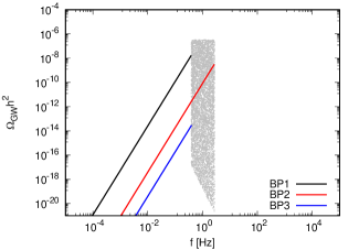
Figure 2: Amplitude $\Omega_{\rm GW}$ and frequency $f$ of the GWs for the benchmark point displayed in Fig. 1. Peak amplitude and peak frequency of the GWs for all allowed $(m_{\rm DM},M_{\rm PBH})$ from particle physics experiments and CMB observations displayed in Fig. 1 are plotted (gray dots).

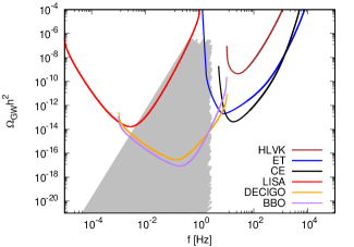
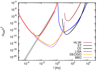
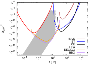
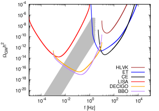
Figure 3: GWs amplitudes and frequencies consistent with the particle physics experiments and CMB observations (gray lines); lines overlapping and appear as filled-in areas. Sensitivity curves of future GW detectors is displayed for comparison. Upper-left panel exhibits all GWs consistent with the particle experiments and CMB observations. Upper-right panel displays only the GWs that can be detected by LISA. Similarly, in the lower-left (lower-right) panel, only GWs detectable by DECIGO and ET are illustrated.

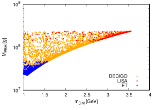
Figure 4: Allowed scotogenic DM and PBH mass ranges upon detecting GWs at DECIGO (orange), LISA (red), and ET (blue).

The constraints on the mass of scotogenic DM and PBH are estimated considering GWs into account.

Figure 2 shows the amplitude $\Omega_{\rm GW}$ and frequency $f$ of the GWs with the peak frequency and peak amplitude

$$(f^{\rm peak}\rm{[Hz]},\Omega_{\rm GW}^{\rm peak})=\begin{cases}(0.387,3.70\times 10^{-8})&\ {\rm BP1}\\ (2.68,6.81\times 10^{-9})&\ {\rm BP2}\\ (0.400,6.41\times 10^{-14})&\ {\rm BP3}\\ \end{cases}$$

at the benchmark point

$$(m_{\rm DM}[{\rm GeV}],M_{\rm PBH}[10^{7}{\rm g}])=\begin{cases}(3.56,23.5)&\ {\rm BP1}\\ (1.06,2.26)&\ {\rm BP2}\\ (1.04,23.4)&\ {\rm BP3}\\ \end{cases}$$

shown in Fig. 1. The peak amplitude and peak frequency of the GWs are plotted for all allowed $(m_{\rm DM},M_{\rm PBH})$ from particle physics experiments and CMB observations (Fig. 1; gray dots).

Recall that the maximum frequency of GWs $f^{\rm peak}$ is determined by $M_{\rm PBH}$ from Eq. (16). Corresponding to the narrow $M_{\rm PBH}$ range in Fig. 1, the allowed maximum frequency $f^{\rm peak}$ shown in Fig. 2 is limited to a narrow range as

$$0.387\lesssim \ f^{\rm peak}\rm{[Hz]}\ \lesssim 2.76,$$

$$2.21\times 10^{-21}\lesssim \Omega_{\rm GW}^{\rm peak} \lesssim 3.25\times 10^{-7}.$$ (23)

Figure 3 illustrates the range of GW amplitudes and frequencies consistent with the particle experiments and CMB observations, represented by gray lines (which overlap to appear as filled-in areas). Not all data from numerical calculations are displayed in the figure; they are selectively thinned to minimize the electronic file size. Additionally, the sensitivity curves of future GW detectors are presented for comparative analysis. The upper-left panel depicts all GWs that are consistent with particle physics experiments and CMB observations, while the upper-right panel isolates only those GWs detectable by the LISA. Similarly, the lower-left and lower-right panels feature GWs solely detectable by the DECIGO and the ET, respectively. These sensitivity curves are plotted based on data from Ref. [141].

The upper-right and lower-right panels of Figure 3 indicate that the GWs observable by LISA and ET are restricted to a narrow frequency range. We will elucidate that the future detection of GWs by these instruments could impose stringent constraints on the masses of scotogenic DM and PBHs, constraints that are hitherto unattained.

Note that in Fig. 3, the GWs under consideration in this study are precluded from existing within the sensitivity regions of the HLVK and the CE. Nevertheless, a plethora of GW sources, other than PBH density fluctuations in the PBH-dominated universe, do exist. Thus, even if GWs were detected in future observations by HLVK and CE, the proposed scenario in this study would not be immediately invalidated. Additionally, GW components originating from sources other than PBH density fluctuations might coexist in the GW region studied herein, rendering the obtained constraints to be conservative.

Figure 4 illustrates the allowed mass ranges for scotogenic DM and PBHs when GWs are detected by DECIGO (depicted in orange), LISA (in red), and ET (in blue). The allowed mass range for BBO closely resembles that for DECIGO and is, therefore, omitted for brevity. In case the GWs are detected by DECIGO, the allowed masses for scotogenic DM and PBHs can be expressed as

$$\begin{aligned} 1.00\lesssim m_{\rm DM}[{\rm GeV}]\lesssim 3.57,\\ 2.22\lesssim M_{\rm PBH}[10^{7}{\rm g}]\lesssim 23.5,\end{aligned}\qquad{\rm(DECIGO)},$$ (24)

which refers to the same constraint derived from particle physics experiments and CMB observations in Eq.(20). Therefore, GWs observations by DECIGO will not provide stringent constraints on the masses of scotogenic DM and PBH.

This DECIGO situation alters dramatically for LISA and ET. The allowed scotogenic DM and PBH mass range can be revised as

$$\begin{aligned} 1.03\lesssim m_{\rm DM}[{\rm GeV}]\lesssim 3.55,\\ 13.2\lesssim M_{\rm PBH}[10^{7}{\rm g}]\lesssim 23.5,\end{aligned}\qquad{\rm(LISA)}$$ (25)

when GWs are detected in LISA. Only the relatively large PBH masses, around $10^{8}$ g, are allowed. By contrast, when GWs are detected by ET, the allowed masses are

$$\begin{aligned} 1.00\lesssim m_{\rm DM}[{\rm GeV}]\lesssim 1.58,\\ 2.22\lesssim M_{\rm PBH}[10^{7}{\rm g}]\lesssim 4.61,\end{aligned}\qquad{\rm(ET)}.$$ (26)

Only the extremely limited regions in which both DM and PBH masses are relatively small are allowed.

IV Summary

The scotogenic DM is a widely studied DM candidate that is produced by thermal processes as well as by the evaporation of PBHs. The mass of scotogenic DM and PBHs could be constrained by particle physics experiments and CMB observations.

Recent reports indicated that the curvature fluctuations of PBHs at the PBH-dominated epoch in the early universe can be a source of the so-called induced GWs.

In this study, we demonstrated that stringent constraints on the mass of scotogenic DM and PBHs can be obtained from the detection of the induced GWs in LISA and ET. Especially, when GWs are detected by ET, the allowed region of mass of scotogenic DM and PBH are stringently limited at $m_{\rm DM}\simeq\mathcal{O}(1)$ GeV and $M_{\rm PBH}\simeq\mathcal{O}(10^{7})$ g.

Finally, we comment that the amplitude of the induced GWs is extremely sensitive to the PBH mass spectrum [114, 112, 142]. The findings presented herein are contingent upon a monochromatic mass spectrum, and might be subject to modification if an extended mass function is considered.

References

- [1] E. Ma, Phys. Rev. D 73, 077301 (2006).
- [2] D. Suematsu, T. Toma, and T. Yoshida, Phys. Rev. D 79, 093004 (2009).
- [3] D. Suematsu, T. Toma, and T. Yoshida, Phys. Rev. D 82, 013012 (2010).
- [4] T. Hambye, K. Kannike, E. Ma, and M. Raidal, Phys. Rev. D 75, 095003 (2007).
- [5] Y. Farzan, Phys. Rev. D 80, 073009 (2009).
- [6] Y. Farzan, Mod. Phys. Lett. A 25, 2111 (2010).
- [7] Y. Farzan, Int. J. Mod. Phys. A 26, 2461 (2011).
- [8] S. Kanemura, O. Seto, and T. Shimomura, Phys. Rev. D 84, 016004 (2011).
- [9] D. Schmidt, T. Schwetz, and T. Toma, Phys. Rev. D 85, 073009 (2012).
- [10] Y. Farzan and E. Ma, Phys. Rev. D 86, 033007 (2012).
- [11] M. Aoki, M. Duerr, J.Kubo, and H.Takano, Phys. Rev. D 86, 076015 (2012).
- [12] D. Hehn and A. Ibarra, Phys. Lett. B 718, 988 (2013).
- [13] P. S. Bhupal Dev and A. Pilaftsis, Phys. Rev. D 86, 035002 (2012).
- [14] P. S. Bhupal Dev and A. Pilaftsis, Phys. Rev. D 87, 053007 (2013).
- [15] S. S. C. Law and K. L. McDonald, J. High Energy Phys. 09, 092 (2013).
- [16] S. Kanemura, T. Matsui, and H. Sugiyama, Phys. Lett. B 727, 151 (2013).
- [17] M. Hirsch, R. A. Lineros, S. Morisi, J. Palacio, N. Rojas, and J. M. F.Valle, J. High Energy Phys. 10, 149 (2013).
- [18] D. Restrepo, O. Zapata, and C. E. Yaguna, J. High Energy Phys. 11, 011 (2013).
- [19] S.-Y. Ho and J. Tandean, Phys. Rev. D 87, 095015 (2013).
- [20] M. Lindner, D. Schmidt, and A. Watanabe, Phys. Rev. D 89, 013007 (2014).
- [21] H. Okada and K. Yagyu, Phys. Rev. D 89, 053008 (2014).
- [22] H. Okada and K. Yagyu, Phys. Rev. D 90, 035019 (2014).
- [23] V. Brdar, I. Picek, and B. Radovčić, Phys. Lett. B 728, 198 (2014).
- [24] T. Toma and A. Vicente, J. High Energy Phys. 01, 160 (2014).
- [25] S.-Y. Ho and J. Tandean , Phys. Rev. D 89, 114025 (2014).
- [26] G. Faisel, S.-Y. Ho and J. Tandean , Phys. Lett. B 738, 380 (2014).
- [27] A. Vicente and C. E. Yaguna, J. High Energy Phys. 02, 144 (2015).
- [28] D. Borah, Phys. Rev. D 92, 075005 (2015).
- [29] W. Wang and Z. L. Han, Phys. Rev. D 92, 095001 (2015).
- [30] J. Kubo, E. Ma, and D. Suematsu, Phys. Lett. B 642, 18 (2006).
- [31] S. Fraser, C. Kownacki, E. Ma, and O. Popov, Phys. Rev. D 93, 013021 (2016).
- [32] R. Adhikari, D. Borah, and E. Ma, Phys. Lett. B 755, 414 (2016).
- [33] E. Ma, Phys. Lett. B 755, 348 (2016).
- [34] A. Arhrib, C. Boehm, E. Ma, and T. C. Yuan, J. Cosmol. Astropart. Phys. 04, 049 (2016).
- [35] H. Okada, N. Okada, and Y. Orikasa, Phys. Rev. D 93, 073006 (2016).
- [36] A. Ahriche, K. L. McDonald, S. Nasri, and I. Picek, Phys. Lett. B 757, 399 (2016).
- [37] W. B. Lu, and P. H. Gu, J. Cosmol. Astropart. Phys. 05, 040 (2016).
- [38] Y. Cai and M. A. Schmidt, J. High Energy Phys. 05, 028 (2016).
- [39] A. Ibarra, C. E. Yaguna, and O. Zapata, Phys. Rev. D 93, 035012 (2016).
- [40] M. Lindner, M. Platscher, and C. E. Yaguna, Phys. Rev. D 94, 115027 (2016).
- [41] A. Das, T. Nomura, H. Okada, and S. Roy, Phys. Rev. D 96, 075001 (2017).
- [42] S. Singirala, Chin. Phys. C 41, 043102 (2017).
- [43] T. Kitabayashi, S. Ohkawa, and M. Yasuè, Int. J. Mod. Phys. A 32, 1750186 (2017).
- [44] A. Abada and T. Toma, J. High Energy Phys. 04, 030 (2018).
- [45] S. Baumholzer, V. Brdar, and P. Schwaller, J. High Energy Phys. 08, 067 (2018).
- [46] A. Ahriche, A. Jueid, and S. Nasri, Phys. Rev. D 97, 095012 (2018).
- [47] T. Hugle, M. Platscher, and K. Schmitz, Phys. Rev. D 98, 023020 (2018).
- [48] T. Kitabayashi, Phys. Rev. D 98, 083011 (2018).
- [49] M. Reig, D. Restrepo, J. W. F. Valle and O. Zapata, Phys. Lett. B 790, 303 (2019).
- [50] A. Ahriche, A. Arhrib, A. Jueid, S. Nasri, and A. de la Puente, Phys. Rev. D 101, 035038 (2020).
- [51] G. Faisel, S.-Y. Ho, and J. Tandean, Phys. Lett. B 738, 380 (2014).
- [52] T. de Boer, M. Klasen, C. Rodenbeck, and S. Zeinstra, Phys. Rev. D 102, 051702 (2020).
- [53] T. Kitabayashi, Int. J. Mod. Phys. A 36, 2150139 (2021).
- [54] T. Kitabayashi, Prog. Theor. Exp. Phys. 2022, 033B02 (2022).
- [55] B. J. Carr, Astrophys. J. 201, 1 (1975).
- [56] B. Carr and F. Kühnel, Annu. Rev. Nucl. Part. Sci. 70, 355 (2020).
- [57] B. Carr, K. Kohri, Y. Sendouda, and J. Yokoyama, Rep. Prog. Phys. 84, 116902 (2021).
- [58] J. Auffinger, Prog. Part. Nucl. Phys. 131, 104040 (2023).
- [59] S. W. Hawking, Commn. Math. Phys. 43, 199 (1975).
- [60] N. F. Bell and R. R. Volkas, Phys. Rev. D 59, 107301 (1999).
- [61] A. M. Green, Phys. Rev. D 60, 063516 (1999).
- [62] M. Y. Kholpov and A. B. J. Grain, Class. Quant. Grav. 23, 1875 (2006).
- [63] D. Baumann, P. Steinhardt, and N. Turok, arXiv:hep-th/0703250 (2007).
- [64] D.-C. Dai, K. Freese and D. Stojkovic, J. Cosmol. Astropart. Phys. 06, 023 (2009).
- [65] T. Fujita, K. Harigaya, M. Kawasaki, and R. Matsuda, Phys. Rev. D 89, 103501 (2014).
- [66] R. Allahverdi, J. Dent, and J. Osinski, Phys. Rev. D 97, 055013 (2018).
- [67] O. Lennon, J. March-Russell, R. Petrossian-Byrne, and H. Tillim, J. Cosmol. Astropart. Phys. 04, 009 (2018).
- [68] L. Morrison, S. Profumo and Y. Yu, J. Cosmol. Astropart. Phys. 05, 005 (2019).
- [69] D. Hooper, G. Krnjaic, and S. D. McDermott, J. High Energy Phys. 08, 001 (2019).
- [70] I. Masina, Eur. Phys. J. Plus 135, 552 (2020).
- [71] N. Bernal and Ó. Zapata, J. Cosmol. Astropart. Phys. 03, 007 (2021).
- [72] I. Baldes, Q. Decant, D. C. Hooper, and L. Lopez-Honorez, J. Cosmol. Astropart. Phys. 08, 045 (2020).
- [73] P. Gondolo, P. Sandick, and B. S. E. Haghi, Phys. Rev. D 102, 095018 (2020).
- [74] N. Bernal and Ó. Zapata, Phys. Lett. B 815, 136129 (2021).
- [75] S. Datta, A. Ghosal, and R. Samanta, J. Cosmol. Astropart. Phys. 08, 021 (2021).
- [76] A. Chaudhuri and A. Dolgov, J. Exp. Theor. Phys 133, 552 (2021).
- [77] T. Kitabayashi, Prog. Theor. Exp. Phys. 2022, 123B01 (2022).
- [78] T. Kitabayashi, Int. J. Mod. Phys. A 37, 2250181 (2022).
- [79] P. Sandick, B. Shams Es Haghi, and K. Sinha, Phys. Rev. D 104, 083523 (2021).
- [80] A, Cheek, L, Heutier, Y. F. P.-Gonzalez, and J. Turner, Phys. Rev. D 105, 015022 (2022).
- [81] S. J. Das, D. Mahanta, and D. Borah, arXiv:2014.14496 (2021).
- [82] M. J. Baker and A. Thamm, SciPost Phys. 12, 150 (2022).
- [83] J. Auffinger, I. Masina, and G. Orlando, Eur. Phys. J. Plus 136, 261 (2021).
- [84] K. Tomita, Prog. Theor. Phys. 37, 831 (1967).
- [85] S. Matarrese, O. Pantano, and D. Saez, Phys. Rev. D 47, 1311 (1993).
- [86] S. Matarrese, O. Pantano, and D. Saez, Phys. Rev. Lett. 72, 320 (1994).
- [87] S. Matarrese, S. Mollerach, and M. Bruni, Phys. Rev. D 58, 043504 (1998).
- [88] H. Noh and J. -c. Hwang, Phys. Rev. D 69, 104011 (2004).
- [89] C. Carbone and S. Matarrese, Phys. Rev. D 71, 043508 (2005).
- [90] K. Nakamura, Prog. Theor. Phys. 117, 17 (2007).
- [91] K. N. Ananda, C. Clarkson, and D. Wands, Phys. Rev. D 75, 123518 (2007).
- [92] D. Baumann, P. J. Steinhardt, K. Takahashi, and K. Ichiki, Phys. Rev. D 76, 084019 (2007).
- [93] B. Osano, C. Pitrou, P. Dunsby, J.-P. Uzan, and C. Clarkson, J. Cosmol. Astropart. Phys. 04, 003 (2007).
- [94] J. R. Espinosa, D. Racco, and A. Riotto, J. Cosmol. Astropart. Phys. 09, 012 (2018).
- [95] K. Kohri and T. Terada, Phys. Rev. D 97, 123532 (2018).
- [96] G. Domènech, Int. J. Mod. Phys. D 29, 2050028 (2020).
- [97] G. Domènech, S. Pi, and M. Sasaki, J. Cosmol. Astropart. Phys. 08, 017 (2020).
- [98] LIGO Scientific collaboration, Class. Quant. Grav. 27, 084006 (2010).
- [99] LIGO Scientific collaboration, Class. Quant. Grav. 32, 074001 (2015).
- [100] VIRGO collaboration, Class. Quant. Grav. 32, 024001 (2015).
- [101] KAGRA collaboration, Class. Quant. Grav. 29, 124007 (2012).
- [102] M. Punturo, et al., Class. Quant. Grav. 27, 194002 (2010).
- [103] M. Maggiore, et al., J. Cosmol. Astropart. Phys. 03, 050 (2020).
- [104] LIGO Scientific collaboration, Class. Quant. Grav. 34, 044001 (2017).
- [105] LISA collaboration, arXiv:1702.00786 (2017).
- [106] N. Seto, S. Kawamura, and T. Nakamura, Phys. Rev. Lett. 87, 221103 (2001).
- [107] S. Kawamura, et al., Class. Quant. Grav. 23, S125 (2006).
- [108] J. Crowder and N. J. Cornish, Phys. Rev. D 72, 083005 (2005).
- [109] G. M. Harry, P. Fritschel, D. A. Shaddock, W. Folkner and E. S. Phinney, Class. Quant. Grav. 23, 4887 (2006) [Erratum ibid. 23 (2006) 7361].
- [110] T. Papanikolaou, V. Vennin, and D. Langlois, J. Cosmol. Astropart. Phys. 03, 053 (2021).
- [111] K. Inomata, K. Kohri, T. Nakamura, and T. Terada, Phys. Rev. D 100, 043532 (2019).
- [112] G. Domènech, C. Lin, and M. Sasaki, J. Cosmol. Astropart. Phys. 04, 062 (2021). [Erratum ibid. 11 (2021) E01].
- [113] G. Domènech, V. Takhistov, and M. Sasaki, Phys. Lett. B 823, 136722 (2021).
- [114] D. Borah, S. J. Das, R. Samanta, and F. R. Urban, J. High Energy Phys. 03, 127 (2023).
- [115] P. Minkowski, Phys. Lett. B 67, 421 (1977).
- [116] T. Yanagida, in Proceedings of the Workshop on the Unified Theory and Baryon Number in the Universe, KEK, 1979, edited by O. Sawada and A. Sugamoto (KEK report 79-18, 1979), p.95.
- [117] M. Gell-Mann, P. Ramond, and R. Slansky, in Supergravity, Proceedings of the Supergravity Workshop, Stony Brook, 1979, edited by P. van Nieuwenhuizen and D.Z. Freedmann (North-Holland, Amsterdam 1979), p.315.
- [118] S. L. Glashow, in Proceedings of the 1979 Cargse Summer Institute on Quarks and Leptons, Cargse, 1979, edited by M. Lvy, J.-L. Basdevant, D. Speiser, J. Weyers, R. Gastmans, and M. Jacob (Plenum Press, New York, 1980), p.687.
- [119] R. N. Mohapatra and G. Senjanovic̀, Phys. Rev. Lett. 44, 912 (1980).
- [120] K. Griest and D. Seckel, Phys. Rev. D 43, 3191 (1991).
- [121] E. W. Kolb and M. S. Turner, Front. Phys. 69, 1 (1990).
- [122] N. Aghanim, et al. (Planck Collaboration), Astron. Astrophys. 641, A6 (2020).
- [123] J. Garcia-Bellido, A. D. Linde, and D. Wands, Phys. Rev. D 54, 6040 (1996).
- [124] M. Kawasaki, N. Sugiyama, and T. Yanagida, Phys. Rev. D 57, 6050 (1998).
- [125] J. Yokoyama, Phys. Rev. D 58, 83510 (1998).
- [126] M. Kawasaki, T. Takayama, M. Yamaguchi, and J. Yokoyama, Phys. Rev. D 74, 043525 (2006).
- [127] T. Kawaguchi, M. Kawasaki, T. Takayama, M. Yamaguchi, and J. Yokoyama, Mon. Not. R. Astron. Soc. 388, 1426 (2008).
- [128] K. Kohri, D.H. Lyth, and A. Melchiorri, J. Cosmol. Astropart. Phys. 04, 038 (2008).
- [129] M. Drees and E. Erfani, J. Cosmol. Astropart. Phys. 04, 005 (2011).
- [130] C.-M. Lin and K.-W. Ng, Phys. Lett. B 718, 1181 (2013).
- [131] A. Linde, S. Mooij, and E. Pajer, Phys. Rev. D 87, 103506 (2013).
- [132] S. Hamdan and J. Unwin, Int. J. Mod. Phys. A 33, 29 (2018).
- [133] C. Caprini and D. G. Figueroa, Class. Quant. Grav. 35, 163001 (2018).
- [134] I. Esteban, M. C. Gonzalez-Garcia, M. Maltoni, T. Schwetz, and A. Zhou, J. High Energy Phys. 09, 178 (2020); “NuFit 5.2 (2022)”, www.nu-fit.org.
- [135] J. A. Casas and A. Ibarra, Nucl. Phys. B 618, 171 (2001).
- [136] K. Kohri and J. Yokoyama, Phys. Rev. D 61, 023501 (1999).
- [137] M. Kawasaki, K. Kohri, and N. Sugiyama, Phys. Rev. D 62, 023506 (2000).
- [138] M. Agostini, et al. (GERDA Collaboration), Science 365, 1445 (2019).
- [139] F. Capozzi, E. D. Valentino, E. Lisi, A. Marrone, A. Melchiorri and A. Palazzo, Phys. Rev. D 101, 116013 (2020).
- [140] A. M. Baldini, et al., (MEG Collaboration), Eur. Phys. J. C 76, 434 (2016).
- [141] K. Schmitz, J. High Energy Phys. 01, 097 (2021).
- [142] T. Papanikolaou, J. Cosmol. Astropart. Phys. 10, 089 (2022).