Soft-Dropout: A Practical Approach for Mitigating Overfitting in Quantum Convolutional Neural Networks

Abstract

Quantum convolutional neural network (QCNN), an early application for quantum computers in the NISQ era, has been consistently proven successful as a machine learning (ML) algorithm for several tasks with significant accuracy. Derived from its classical counterpart, QCNN is prone to overfitting. Overfitting is a typical shortcoming of ML models that are trained too closely to the availed training dataset and perform relatively poorly on unseen datasets for a similar problem. In this work we study the adaptation of one of the most successful overfitting mitigation method, knows as the (post-training) dropout method, to the quantum setting. We find that a straightforward implementation of this method in the quantum setting leads to a significant and undesirable consequence: a substantial decrease in success probability of the QCNN. We argue that this effect exposes the crucial role of entanglement in QCNNs and the vulnerability of QCNNs to entanglement loss. To handle overfitting, we proposed a softer version of the dropout method. We find that the proposed method allows us to handle successfully overfitting in the test cases.

I Introduction

Quantum machine learning (QML) has shown great promise on several prototypes of NISQ devices, presenting significant accuracy over several different datasets, see e.g.,  [1, 2] and references therein. It has been proven effective even on a limited number of available qubits, not only on simulated devices but even when tested on noise-prone quantum information processing devices, as seemingly proven difficult in the case presented in [3]. As most of QML models have been derived from the classical machine learning (ML) models, with adaptations over the functioning being operable on quantum devices, these algorithms pose similar challenges as found in their classical counterparts. One of the setbacks of ML models, classical and quantum included, is overfitting, causing models to underperform on average when presented with external data outside the training set for the same problem. Due to its importance, the problem of overfitting has been studied extensively in the classical ML literature, and several methods have been proposed and implemented to mitigate it, see e.g., [4] and Sec. II for a brief overview. Very generally, there are two ways one can approach the problem of overfitting. In the first approach we combat overfitting before or during the training process. This can be done, for example, by data augmentation or regularization techniques [4]. Complementary to this approach, overfitting can be treated post-training by changing the trained parameters to compensate for overfitting. One such method for handling overfitting in neural networks (NN) architectures is neuron dropout [5]. In this method, a new NN is created from the trained NN by removing (dropping out) a few neurons from the network. Due to its simplicity and proven applicability in a wide range of NNs, dropout became one of the most popular techniques to handle overfitting in the classical ML paradigm. While pre-training methods can be effective to a certain extent, they may not fully eliminate the problem of overfitting since during the training, the model may potentially learn patterns that are specific to that data and may not generalize well. In contrast, post-training methods generally allow for a more comprehensive analysis of the trained model’s behavior and performance, resulting in fine-tuning the models and improving generalization.

In contrast to the classical setting, there has been much less investigation as to how to address the problem of overfitting in QML models. While pre-training methods such as data augmentation or early stopping may have been implemented in the QML setting, to the best of our knowledge there has been no systematic study of the problem of overfitting in QML models. In this paper, we study the problem of overfitting in QML models and propose a post-training method to mitigate it. Specifically, we focus on the dropout method as a deterrent for overfitting and for concreteness, and since it is one of the widely-used QML architectures, we concentrate on quantum convolutional neural networks (QCNNs) [6]. As we discuss in more detail in the following sections, we find that a straightforward generalization of the dropout method to the quantum setting can cause QCNN models to lose their prediction capabilities on the trained data, let alone improving overfitting. As we shall argue, this result can be traced back to the way QCNNs are designed and to the crucial role of entanglement in their performance and success. Therefore, we propose a new method that is based on a “softer” version of the post-training dropout method termed soft-dropout, an overfitting deterrent. This method, as we will show, provides excellent performance for suppressing overfitting in QCNN for the tested cases.

The paper is organized as follows: In Sec. II, we discuss the problem of overfitting and the classical techniques for mitigating it. In Sec. III we present the various techniques we tested and developed to mitigate overfitting in QCNNs. In Sec. IV we present our numerical experimental results using these techniques. We offer conclusions and outlook in Sec. V.

II Overfitting and its mitigation in classical neural networks

Before considering the problem of overfitting in the quantum setting, in the following section, we take a closer look at this problem as it is manifested in the classical setting and the current methods for mitigating it [4].

Overfitting is one of the common problems noticed in ML and statistical modeling, where a model performs exceptionally well on the training data but needs to be generalized to new, unseen data. It occurs when the model learns the noise and random fluctuations in the training data in addition to the underlying patterns and relationships. When a model overfits the training data, it becomes too complex and captures the idiosyncrasies of the training data, leading to poor performance on any new data. In practice, overfitting is manifested as a relatively poor performance of a model, in terms of its prediction accuracy, on validation data. Therefore, model overfitting is a problem that undermines the very essence of the learning task, i.e., generalizability. For this reason, a lot of efforts have been devoted to developing methods and techniques to handle overfitting and make sure that learning models are flexible enough and not overfitted to the training data. We briefly review some of the most popular techniques in what follows, see also [4] and references therein.

Cross-validation is a pre-training technique used to assess the performance and robustness of a model. It involves splitting the data into multiple subsets or folds and training the model on different combinations of these subsets. By evaluating the model’s performance on different folds, cross-validation helps estimate the model’s ability to generalize to new data. It can be easily implemented in classical as well as quantum ML models (we have implemented it in our numerical experiments). Increasing the training data size by augmenting it can also help alleviate overfitting. Data augmentation techniques involve generating additional training samples by applying transformations, such as rotations, translations, or distortions, to the existing data. This introduces more variation and diversity, helping the model to generalize better. This method of avoiding overfitting is highly dependent on the availability of data and is easily transferable to QML since it is not related to the ML aspect but the data prepossessing part and is considered during the experimental process.

Regularization is another popular pre-training overfitting prevention technique. In general terms, it avoids overfitting by adding a penalty term to the loss function during training. In this way, regularization introduces a bias into the model, discouraging overly complex solutions. $L1$ and $L2$ regularization are commonly used methods. $L1$ regularization (Lasso) adds the absolute value of the coefficients to the loss function, promoting sparsity. $L2$ regularization (Ridge) adds the squared value of the coefficients, which tends to distribute the impact across all features. Overfitting can occur when the model has access to many irrelevant or redundant features. Feature selection techniques aim to identify and retain only the most informative and relevant features for model training. This can be done through statistical methods, such as univariate feature selection or recursive feature elimination, or using domain knowledge and expert intuition. Feature selection has been implemented in the QML setting and has proven to be useful [7].

In addition to the aforementioned methods, the complexity of a model plays a crucial role in determining the risk of overfitting. Simplifying the model architecture or reducing the number of parameters can mitigate overfitting. Techniques such as reducing the number of hidden layers, decreasing the number of neurons, or using simpler model architectures, like linear models or decision trees, can help control the complexity and prevent overfitting.

Finally, we mention dropout. Dropout is a regularization technique specific to NNs. It is one of the most popular methods for mitigating overfitting in classical NNs due to its simplicity and performance [4, 5]. Dropout can be implemented in two ways: one is during the training process, and another method would be after getting a trained model. During training, dropout randomly disables a fraction of the neurons in each layer, forcing the network to learn redundant representations and reducing the reliance on specific neurons. For post-training methods of dropout, typically a few percent of neurons are dropped at random from a trained NN. This process is repeated, with different realization, until the least overfitted model is found. The dropout method is known to help to prevent overfitting by making the network more globally robust and less sensitive to individual neurons [5].

In this work, we adjust the dropout method to the QCNNs’ setting and experimentally test it. We find that due to quantum entanglement, the dropout method does not carry over in its simple form to the quantum setting. Rather, we propose a softer version of dropout, as we describe in the next section. We found that the soft-dropout method performs very well in mitigating overfitting in several QCNN numerical experiments. The reason for proposing a post-training method for a QCNN model is as a prevention technique to tackle overfitting even after all previous measures are considered prior to training the model and overfitting is still observed.

III Methods and Techniques

Before presenting the results from our numerical experiments, we devote this section to providing an overview of the main tools and techniques we used and developed in this work.

III.1 The QCNN architecture

QCNNs are essentially variational quantum algorithms [6, 8]. Similar to their classical counterparts, QCNN is designed and used for solving classification problems (supervised and unsupervised paradigms have been studied in this context) [9]. They were proposed to be well-fitted for NISQ computing due to their intrinsically shallow circuit depth. It was shown that due to unique quantum phenomena, such as superposition and entanglement, QCNN can provide better prediction statistics using less training data than classical ones in certain circumstances [10].

Due to the noise and technical challenges of building quantum hardware, the size of quantum circuits that can be reliably executed on NISQ devices is limited. Thus, the encoding schemes for high dimensional data usually require a number of qubits that are beyond the current capabilities of quantum devices. Therefore, classical dimensionality reduction techniques are particularly useful in the near-term application of QML techniques. In this work, the classical data was pre-processed using two dimensionality reduction techniques, namely Principal Component Analysis (PCA) [11] and Autoencoding (AutoEnc) [12]. Autoencoders are capable of modeling complex non-linear functions, whereas PCA is a simpler linear transformation that helps in cheaper and faster computation.

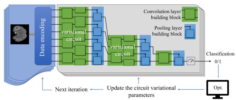
Figure 1: General QCNN architecture. The QCNN includes three key components: A feature map, a parametric quantum circuit that includes concatenated convolution and pooling layers, and a measurement followed by an optimization unit. In this work the convolution and the pooling layers are constructed from two-qubit gates (building blocks). Examples of the building blocks we used are given in Fig. LABEL:fig:conv.

A generic QCNN is composed of a few key components [6, 8], as illustrated in Fig. 1. The first component is data encoding, also known as a quantum feature map. In classical ML, feature maps are used to transform input data into higher-dimensional spaces, where the data can be more easily separated or classified. Similarly, a quantum feature map transforms classical data into a quantum state representation. The main idea is to encode the classical data as an entangled state with the possibility of capturing richer and more complex patterns within the data. The quantum feature map is done in practice by applying a unitary transformation to the initial state (typically the all-zero state). In this work, we implemented two of the main feature encoding schemes, amplitude encoding and qubit encoding [6, 8]. In the former, classical data $(x_{1},\ldots,x_{k})\in\mathrm{R}^{k}$ is represented as, generally, an entangled input quantum state $|\psi_{\rm in}\rangle\sim\sum_{i=1}^{k}x_{i}|i\rangle$ (up to normalization), where $|i\rangle$ is a computational basis ket. Amplitude encoding uses a circuit depth of size ${\cal O}(\log N)$ circuit and $N$ qubits [13]. To evaluate the robustness of our dropout method with respect to the feature map, we also used qubit encoding. In this method the input state is a separable state $|\psi_{\rm in}\rangle=\bigotimes_{i=1}^{k}(\cos\frac{x_{i}}{2}|0\rangle+\sin\frac{x_{i}}{2}|1\rangle)$. As such, it uses a constant-depth circuit given by a product of a single-qubit rotation.

The second key component of a QCNN is a parameterized quantum circuit (PQC) [14, 15]. PQCs are composed of quantum gates whose action is determined by the value of a set of parameters. Using a variational algorithm (classical or quantum), the PQC is trained by optimizing the parameters of the gates to yield the highest accuracy in solving the ML task (e.g., classification) on the input data. Typically, in QCNN architectures, the PQC is composed of a repeated sequence of a (parametric) convolution circuit followed by and a (parametric) pooling circuit. The convolution layer is used as the PQC for training a tree tensor network (TTN) [16]. In this work, we used a specific form of the convolution layer, which was proposed and implemented by Hur et al. [8], and that is constructed out of a concatenation of two-qubit gates (building blocks). In Fig. LABEL:fig:conv(a)-(b) we sketch two of the building blocks that we used for convolution layer in our architecture.

The convolution layer is followed by a pooling layer, which reduces the dimensionality of the input data while preserving important features, i.e., the pooling layer applies parameterized (controlled) quantum gates on the sequence of two qubits. To reduce the dimensionality, the control qubits are traced out (assuming they maintain coherence through the computation) while the target qubits continue to the next convolution layer, see Fig. 1. For the implementation of the pooling layer, we used a parameterized two-qubit circuit that consisting of two controlled rotations $R_{z}(\theta_{1})$ and $R_{x}(\theta_{2})$, respectively, each activated when the control qubit is 1 or 0 (filled and open circle in Fig. LABEL:fig:conv(c)). The PQC is followed by a measurement in the computational basis on the last layer of qubits.

Training the QCNN is obtained by successively optimizing the PQC using the input data and their labels by minimizing an appropriate cost function. Here we use the mean squared error (MSE) between predictions and class labels. Given a set of training data $\{|\psi_{i}\rangle,y_{i}\}$ of size $K$, where $|\psi_{i}\rangle$ denotes an initial state and $y_{i}\in\{0,1\}$ denotes their label, the MSE cost function is given by

$$C(\boldsymbol{\theta})=\frac{1}{K}\sum_{i=1}^{K}\Big{(}y_{i}-f_{\boldsymbol{\theta}}(|\psi_{i}\rangle)\Big{)}^{2}.$$ (1)

Here, $f_{\boldsymbol{\theta}}(|\psi_{i}\rangle)$ is the output of QCNN ($f\in\{0,1\}$) which depends on the set of parameters $\boldsymbol{\theta}$ that define the gates of the PQC.

III.2 Dropout

Once the models had been trained, we tested two dropout approaches to mitigate overfitting: a straightforward generalization of the classical dropout method and a ‘softer’ approach.

In the classical setting, post-training dropout is usually implemented by removing a certain percentage of neurons from the network. In a similar vein, in our first approach, we dropped a certain percentage of single-qubit gates (equivalently, replacing a gate with the identity gate) from the trained network. None of the CNOT gates in the convolution layers or the controlled two-qubit gates in the pooling layers were dropped out. As discussed in length in Sec. IV, we found that this dropout method fails catastrophically. Not only did it not help with mitigating overfitting, it substantially reduced the success rates on the trained data.

The second method we implement to mitigate overfitting in QCNNs we termed soft-dropout. Since setting (random, single-qubit) gates to the identity seemed to have a crucial effect on the network’s performance, we hypothesized that tinkering with the trained parameters to a certain degree might provide enough flexibility to the model without hampering its accuracy and predicting capability. In the soft-dropout method, rather than dropping out gates completely, some of the trained parameters are slightly modified. The performance of the slightly modified model was then tested using testing and validation data. The process of changing the trained parameters was done manually to study the effect of the soft-dropout method and the threshold at which the changing parameter falters. We envision the soft-dropout not as a single technique to deter overfitting but as several collections of techniques that can be utilized individually or in combination. Soft-dropout may consist of techniques such as rounding the trained parameters up to certain decimal places, asserting certain values up to a threshold to a common whole number, and setting certain values close to zero, considering their proximity to the number. For the technique of setting values to zero, all the trained parameter values in the list of parameters below a certain floating number value (generally ranging below $|\pm 0.09|$) were changed to float value $0$ by taking the absolute of all the parameters to cover all the values from the positive and negative spectrum of trained parameters. A similar technique was utilized in the case of threshold whole number conversion instead of setting it up to zero; the threshold depended on the point of mitigating overfitting without loss in accuracy dropping, which was found over several manual iterations of finding the least testing-validation accuracy value and not losing the actual testing value significantly. For the round-off method, a built-in Python function for rounding up values up to certain decimal places was used, while not all values were rounded up to certain decimal places as after a certain threshold, a severe drop in accuracy was observed. The threshold for the round-off method was determined by iterating the method until finding the parameters that yield the highest validation accuracy compared to the unmitigated circuit. Results and observations of the soft-dropout method are discussed for all the datasets in Sec. IV.

IV Numerical experiments and results

IV.1 Datasets

Using multiple datasets in ML, including QML, is very useful to increase generalization, robustness, and reliability. It also helps overcome data limitations, introduces variability and heterogeneity, and allows the exploration of different perspectives. In regards to these ideas, we chose to work with three datasets, two of them being image-based medical datasets, Medical MNIST [17] and BraTS [18], while the third was a Stellar dataset [19] consisting of numerical values.

Each dataset was split into three parts: one for training, another for testing, and the last portion for validation. The validation set is used to test the performance of the (trained) QCNN on an unseen dataset and provide a proxy for determining if the model exhibits overfitting and how well we mitigate this problem. Many variations of percentage split were implemented to find the best option for creating the overfitting conditions. This operation was performed for all three datasets. Later, after the split, the testing data was added to the training data to develop the overfitting conditions more prominently. Subsequently, the data were processed using PCA for dimensionality reduction and fitting it to the limited number of qubits (we used 8, 12, and 12 qubits). The classically-processed data was then sent for training on a (simulated) QCNN.

Medical MNIST.— The Medical MNIST dataset consists of 6 classes: Abdominal CT, Breast MRI, Chest CT, Chest X-ray, Hand X-ray, and Head CT. These classes contained around 10000 images, each of size $64\times 64$ pixels. As we are trying to implement binary classification, all possible permutations of classes were tested, and the similarity between Chest CT and Abdominal CT was considered most of the time. Several QCNNs were created to differentiate between the CT images being a Chest CT image or an Abdominal CT image. These two classes were pretty much alike and, hence, challenging to differentiate and were prone to overfitting, see Fig. 3.

Figure 3: Example of Medical MNIST dataset images. Top row: Abdominal CT, bottom row: Chest CT. The similarity between Chest CT and Abdominal CT images implies that they would be hard to classify and in addition, that the learning model may be prone to overfitting.

BraTS 2019.— To validate the uniformity of the proposed dropout approach on different datasets and models, we used another medical dataset for this implementation. The BraTS 2019 dataset was chosen for classification between High-Grade Gliomas (HGG) and Low-Grade Gliomas (LGG) patient MRI images. The BraTS 2019 training dataset has 259 HGG and 76 LGG images. The BraTS multimodal scans are provided in NIfTI file format (.nii.gz) and include the following components: a) native (T1) scans, b) post-contrast T1-weighted (T1Gd) scans, c) T2-weighted (T2) scans, and d) T2 Fluid Attenuated Inversion Recovery (T2-FLAIR) scans. These scans were obtained using diverse clinical protocols and a variety of scanners from a total of 19 different institutions. Due to resource limitations, only one modality, specifically the T2-FLAIR, was considered for the classification of HGG versus LGG. The images were resized to 64 pixels. As depicted in Fig. 4, the resulting images appeared unclear and pixelated, which was expected given the constraints.

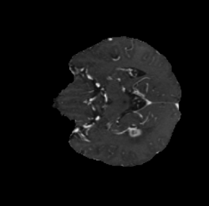
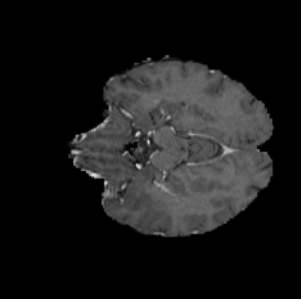
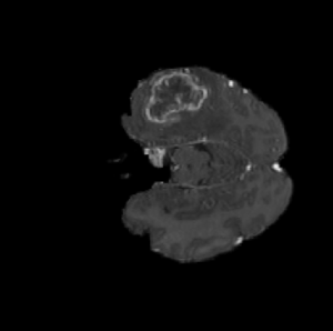
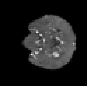
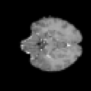
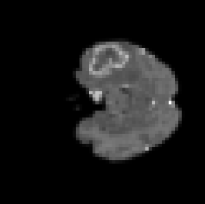
Figure 4: Example of BraTS 2019 dataset brain images The high-resolution brain images at the top row were resized to 64 pixels, bottom row. The resulting images appeared unclear and pixelated which pose a challenge for classification.

Stellar classification dataset (SDSS17).— As both of the prior datasets were image-based, we consider using a dataset in a different format to verify the conclusions devised and ascertain our claims derived from the results. The stellar classification dataset SDSS17 seemingly proved to be a reliable candidate. It consists of 100,000 observations of space taken from the Sloan Digital Sky Survey (SDSS). Every recorded observation was registered in 17 columns defining different values, such as the ultraviolet filter in the photometric system, the green filter in the photometric system, the redshift value based on the increase in wavelength, etc., and one class column identifying the category for being a star, quasar or a galaxy. Out of the 17 available columns, only 8 were used for training the model after the initial data pre-processing (columns containing the ID of equipment and date parameters were removed in order to generalize the object regardless of its position in the sky and the equipment detecting it). Considering the close proximity of the star and quasar data and their difficulty in classifying based on the data available, we considered classifying these two classes using QCNN. As the data consisted of only 8 columns, PCA did not need to be applied to reduce the dimensionality of the data. Hence, all the experiments conducted for the classification of this dataset were limited to 8 qubits. The same process of data splitting was utilized as defined for the previous dataset with few exceptions for the train-test-validation split percentage in order to characterize the overfitting scenario.

IV.2 Results from numerical experiments

All the experimental data generated for this manuscript was generated using the Pennylane software (v0.31) and simulated on a local classical device, considering the total amount of iteration needed to train the QML model and the queuing operations required to complete the process on any of the available quantum computers on the cloud. For optimization purposes, we utilized the Pennylane optimizer Nesterov Momentum Optimizer, considering its merits observed during the initial training of the QML models [20]. The total number of qubits used for this experimentation varied from 8-16 depending upon the dataset used and the complexity of the circuit. PCA, as previously mentioned in Sec. III, was utilized for converting higher dimensionality data onto the number of qubits defined for the QML model.

We verify success in mitigating overfitting in our experiment by two metrics: (1) increasing validation accuracy and (2) reducing the difference between testing and validation accuracy after implementing the dropout method.

IV.2.1 Mitigating overfitting using dropout

The first method we implemented to mitigate overfitting in QCNN is a direct adaptation of (post-training) dropout to the quantum setting, as discussed above. We have applied this method to mitigate overfitting when considering the Medical MNIST dataset. We found that this method has devastating effects on the tested QCNNs. For example, when we implemented this method on an 8-qubit model with a testing accuracy of $95\%$ and validation accuracy of $90\%$, by dropping out only $5\%$ of the single-qubit gates, the accuracy of the QCNN on the testing data was reduced significantly with $77\%$ accuracy being one of the best-performing models and about $2\%$ being the worst-performing. Not only was this method not able to mitigate overfitting by increasing validation accuracy or reducing the gap between the testing and validation accuracy, but it also resulted in dramatically hampering the performance of the network on the trained data. Similar behavior was observed to be robust with respect to the number of single-qubit gates that were dropped out. Particularly, we tested dropping out $1\%$ to $10\%$ of the single-qubit gates and observed a similar drastic drop in performance accuracy. This was contrary to our naïve intuition that a network with many gates, more than the minimum required to accomplish the learning task, should be minimally affected, if at all, by dropping out a few single-qubit gates. To test the effect of the method at its limit, we implemented it by dropping out one (randomly chosen) single-qubit gate out of a model with 78 gates. This experiment resulted in very interesting results. In these cases, the accuracy was plunged to a range of about $46\%$ to $53\%$, which is almost $50-50$ chance in the particular model we have tested. This experimentation bore the conclusion that even deleting a single gate from the circuit of a trained QCNN causes a loss of information gained during the training process.

We hypothesize that entanglement plays a crucial role in this behavior. In classical CNN, where the dropout method is used very successfully, each neuron holds a few bits of information regarding the data it is trained on, and therefore, losing a small fraction of neurons does not affect the overall performance of the entire network. In stark contrast, QCNN is designed to harness entanglement between qubits in our implementation through the concatenation of single-qubit (parameterized) gates and CNOT gates. This means that the information learned about a certain dataset is stored and distributed in the QCNN in a “non-local” way, loosely speaking. Our experiments show that entanglement can be a double-edged sword in quantum NNs: On one hand, it may promote speedup, e.g., in terms of learning rates, but on the other hand, it can lead to a fragile NN, in the sense that removing even a single gate from a trained network may have devastating consequences with respect to its performance. This experiment, therefore, exposes an intrinsic vulnerability of QML, and QCNNs in particular, in comparison to their classical counterpart.

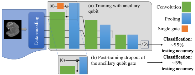
Figure 5: Ancillary qubit dropout experimental setup. The figure depicts the experimental setup used to exemplify the vulnerability of QML models. (a) The QCNN is trained along with an ancillary qubit, which is not part of the feature map. The ancilla qubit takes part in the training via a parameterized rotation ($R_{x}$ or $R_{y}$). We found that this setup results in a testing accuracy of about 95%. (b) After training is completed, removing the single-qubit gate from the ancillary qubit, the model experienced a significant loss in prediction accuracy.

To ascertain the conclusion, we have conducted a set of experiments, schematically shown in Fig. 5. We have constructed a QCNN with 8 qubits and an additional ancillary qubit that does not pass through the feature map but rather is initialized in a computational state (say, $|0\rangle$) as a non-featured attestation to the QCNN circuit. Thus, this qubit does not hold any information about the input data. The ancillary qubit is then passed through a parameterized single-qubit gate (our experiments were done with an $R_{x}$ gate and a $R_{y}$ gate) whose parameters are consistently updated in every iteration of the training cycle along with the rest of the training parameters in the first convolutional layer. The qubit is then entangled with one of the qubits from the circuit with a CNOT gate after the first convolutional layer, and then it is traced out in the following pooling layer. Training this QCNN resulted in 93%-95% testing accuracy (depending on the network building blocks we used). However, by dropping out the parameterized gate of the ancillary qubit, the testing accuracy plunged to order of a few percents. This set of experiments clearly indicates that even though the ancillary qubit was not encoding information about the input data, the mere fact that it is trained and entangled with the rest of the qubits, dropping after training, caused an information loss that resulted in a sharp accuracy drop. These results suggested that while dropping out gates in QCNN may not be a viable method for mitigating overfitting, tinkering with the trained values of the gates parameters may have a more subtle effect and thus can be used for this purpose.

IV.2.2 Mitigating overfitting using soft-dropout

As we discussed above, applying the classically derived method for post-trained dropout resulted in the loss of learned information due dropping of gates. In contrast, encouraging positive results were observed when the soft-dropout method was applied. In these experiments we implemented the method by variations of rounding of the learned parameters and introducing a threshold on the values of the parameters, as prior mentioned in Sec. III.

We summarize our results in Tables 1-3, with respect to the datasets they are associated with. The results clearly indicate that when a model suffers from overfitting (as captured by the lower validation accuracy and also an appreciable difference between test accuracy and validation accuracy), the soft-dropout method not only was successful in reducing the gap between testing and validation accuracy in several test cases, but also helped to increase the model validation accuracy across all of our experiments.

8 qubits
Test Acc.	Validation Acc.	Gap
0.9154	0.7175	0.1979
0.9229	0.8629	0.06
0.9721	0.9136	0.0585
0.9794	0.9447	0.0347
0.9225	0.8770	0.0455
0.9339	0.9039	0.03
0.9675	0.9298	0.0377
0.9464	0.9374	0.009

12 qubits
Test Acc.	Validation Acc.	Gap
0.9008	0.8866	0.0142
0.9545	0.9079	0.0466
0.9560	0.9084	0.0476
0.9620	0.9221	0.0399
0.9345	0.9079	0.0266
0.9360	0.9085	0.0275
0.8450	0.8380	0.0070
0.8637	0.8558	0.0079

Table 1: Results based on Medical MNIST dataset. The table shows the results for the test accuracy, validation accuracy, and the accuracy gap (the difference between the test accuracy and the validation accuracy) for models that were trained with qubits 8 and 12 (in the initial feature map layer). In each pair of rows, the top row (black font) indicates the accuracy obtained from the trained model, while the bottom row (blue/red font) shows the corresponding accuracy when a soft-dropout method was implemented. Blue/red colour indicates success/failure in mitigating overfitting in the corresponding metric. Different pairs of rows correspond to training different models on the same datasets. The results clearly indicate that the soft-dropout method was able to improve validation accuracy on all tested cases and to shrink the accuracy gap by an order of magnitude for certain models.

8 qubits
Test Acc.	Validation Acc.	Gap
0.8728	0.8548	0.018
0.8765	0.8829	-0.0064
0.8543	0.8499	0.0044
0.8655	0.8757	0.0102

12 qubits
Test Acc.	Validation Acc.	Gap
0.8958	0.8859	0.01
0.8996	0.9082	-0.0086
0.8666	0.8645	0.0021
0.8731	0.8793	0.0062

16 qubits
Test Acc.	Validation Acc.	Gap
0.9422	0.9257	0.0165
0.9518	0.9586	-0.0068
0.8972	0.8895	0.0077
0.9127	0.9233	0.0106

Table 2: Results based on BraTS dataset. The format of results is similar to Table 1. for different models that were trained with qubits 8, 12 and 16. For all three numbers of qubits (8, 12, and 16), the validation accuracy after soft-dropout was implemented is higher than without dropout. This suggests that soft-dropout regularization technique helps improve the model’s generalization performance and reduces overfitting.

8 qubits
Test Acc.	Validation Acc.	Gap
0.8866	0.8432	0.0434
0.8890	0.8542	0.0348
0.9456	0.9251	0.0165
0.9456	0.9399	0.0057
0.9500	0.9225	0.0275
0.9455	0.9400	0.0055

Table 3: Results based on Stellar dataset. Results have the same format as in Table 1. The results clearly indicate that soft-dropout was successful in mitigating overfitting, as indicated by higher validation accuracy and smaller gap, as compared to the results with no dropout, across all tested models.

We attempted to devise a systematic way to determine the threshold for rounding up to a number or an absolute value that could be decided for mitigating overfitting after obtaining the trained parameters. Utilizing this method on several trained and overfitted models, we observed that every model had a different threshold which could only be determined after constant testing to find the best fit for tackling the overfitting issue. In addition, a closer observation revealed that the set of parameters which were used to successfully mitigate overfitting were those which fluctuated around a mean value and did not changed much during training. This observation will be explored in more detail in future work.

V Conclusion and Outlook

In this study we focus on addressing the challenge of overfitting in QML setting, specifically, in QCNNs. Overfitting, a common issue in ML models, poses significant obstacles to the generalization performance of QCNNs. To overcome this challenge, we introduced and explored the potential of soft-dropout and compares it to a straightforward application of the dropout method commonly utilized in classical CNNs.

Surprisingly, we found that dropping out even a single parameterized gate from a trained QCNN can results in a dramatic decrease in its performance. This result highlights a vulnerability of QCNNs compared to their classical counterparts. On the other hand the soft-droput approach resulted in encouraging results.

Extensive experimentation is conducted on diverse datasets, including Medical MNIST, BraTS, and Stellar Classification, to evaluate the effectiveness of soft-dropout in mitigating overfitting in QCNNs. Our findings highlight the promising performance of soft-dropout in reducing overfitting and enhancing the generalization capabilities of QCNN models. By fine-tuning the trained parameters through various techniques, notable improvements in accuracy are observed while preserving the integrity of the quantum circuit. Hence, soft-dropout can be considered one of the most viable options to mitigate overfitting in a post-training setting.

We close this section with a few directions for future work. The first direction is developing a systematic approach for determining which, and how, parameters should be tinkered to handle overfitting. Following our initial observation, we believe that identifying those parameters that fluctuate around a mean value during training play an important role for mitigating overfitting.

Another important direction for future work is to investigate the performance of soft-dropout in the presence of experimental noise. Quantum systems are inherently susceptible to noise, which can impact the reliability and effectiveness of quantum operations. Understanding how soft-dropout performs under noisy conditions will contribute to the development of robust QCNN models that can operate in realistic quantum computing environments.

Another aspect that requires further exploration is the scalability and performance of soft-dropout in larger QCNN models. As quantum hardware continues to advance, larger and more complex QCNN architectures become feasible. Evaluating the behavior and effectiveness of soft-dropout in handling larger quantum circuits will provide insights into its scalability and potential challenges in maintaining regularization benefits.

By pursuing these research directions, we can advance the field of QML and enhance the practical deployment of QCNN models. Overcoming overfitting challenges is crucial for ensuring the reliability and effectiveness of QCNNs in real-world applications, unlocking their potential to make significant contributions in various domains.