Extreme first passage times for populations of identical rare events

Abstract

A collection of identical and independent rare event first passage times is considered. The problem of finding the fastest out of $N$ such events to occur is called an extreme first passage time. The rare event times are singular and limit to infinity as a positive parameter scaling the noise magnitude is reduced to zero. In contrast, previous work has shown that the mean of the fastest event time goes to zero in the limit of an infinite number of walkers. The combined limit is studied. In particular, the mean time and the most likely path taken by the fastest random walker are investigated. Using techniques from large deviation theory, it is shown that there is a distinguished limit where the mean time for the fastest walker can take any positive value, depending on a single proportionality constant. Furthermore, it is shown that the mean time and most likely path can be approximated using the solution to a variational problem related to the single-walker rare event.

1 Introduction

Stochasticity is an ingredient used in a mathematical model best used when it imbues a dynamical system with behavior that a simpler deterministic model lacks. This is best seen when the connection between stochastic and deterministic is explicit through a law of large number limit, in which the noise, whatever its sources, vanishes in a so called weak-noise limit. For simplicity, we will suppose that this limit is characterized by a positive nondimensional parameter, $\epsilon>0$, where in the limit $\epsilon\to 0^{+}$, the stochastic process converges to a deterministic dynamical system. For any behavior that exists in the stochastic model but not the deterministic, this limit is singular. The random time over which an event that characterizes this behavior occurs—commonly called a first passage time or hitting time—diverges to infinity as $\epsilon\to 0^{+}$. Events of this type are often called rare events. Their study is informed through exponential asymptotic analysis, namely large deviation theory [6, 4].

There are many situations, particularly those involving exponential proliferation, where it is not the mean first passage time of a single event that is of interest, rather it is the first out of $N$ identical rare events to occur that is relevant [32]. For example, the dynamics of the initial outbreak in an epidemic are highly sensitive to when and where the first infection occurs [36]. For another example, suppose that a tumor is comprised of cells with a single common ancestor. In this case, the first-to-arrive random walker is the first cell to accumulate enough mutations to cause uncontrolled proliferation [9]. Another example is given by predator-prey dynamics where the prey is sufficiently skilled at evading predators that predation is a rare event [13]. In the scenario where a number of predators are introduced to potential prey at the same time (e.g., a school of fish), any given predator would successfully capture a prey a certain way, perhaps skillfully. We might imagine a very different sequence of events for the first predator to eat since this is an event that is doubly rare, in some sense.

Many examples can be found in the calcium signalling literature. The binding of calcium to buffers in exocytosis can be characterized as a first-passage-time problem for a large number of stochastic walkers [33, 23]. Similarly calcium waves in the cell are often kicked off by the stochastic opening of a single channel [30].

There are many examples of bacteria entering a dormant state to avoid the harmful effects of an antibiotic, which kill during cell division. In some cases, switching into and out of the dormant state is governed by a rare event in a certain gene regulatory circuit [26, 25]. Once the antibiotics are no longer present, switching out of this state allows the dormant subpopulation to begin proliferating once again, driven by the first bacterium to make the switch.

The problem can be stated succinctly as follows. Given $N$ independent and identical random walkers (assumed to be continuous time Markov processes) together with a first passage time event characterized by the random variable $\tau>0$, what is the mean of $\tau^{N}_{\rm first}=\min_{n}\{\tau_{n},n=1,\ldots,N\}$? Early work on the statistics of extreme diffusion problems such as these was done by Varadhan [34], and it is known that $\mathbb{E}[\tau^{N}_{\rm first}]$ scales like $C/\log(N)$ as $N\to\infty$, where the constant $C$ depends on the statistics of the single first passage time. This paper focusses on what happens in the dual limit $N\to\infty$ and $\epsilon\to 0^{+}$: i.e. when the mean of the individual first passage times blows up (i.e., $\mathbb{E}[\tau]\to\infty$).

Holcman et al recently proposed extreme first passage times as a useful characterization of biological processes, particularly at the level of cellular physiology, for example, synaptic transmission [23], and the activation of genes by transcription factors [31]. Lawley et al [14, 15, 17] have recently studied the extreme first-passage-time statistics of a large number of random walkers in a range of scenarios. Most of these studies concern situations where $N$ is the dominant asymptotic parameter. That is, it is assumed that the magnitude of the noise experienced by an individual walkers is $O(1)$, and it is determined how the optimal trajectory and first-hitting-time is changes as $N\to\infty$, often using the theory of extreme value statistics [1]. A problem with this approach is that it implies that the first-hitting-particle almost instantaneously hits the target. It goes there so quickly that the effect of advection is negligible. Indeed some scholars have argued that large jumps of Brownian motions such as this are unphysical [12].

In fact, Lawley and Madrid [19] have extended these works to also consider the effect of small noise. Relevant to our paper, they argue that the relative benefit of increased numbers of walkers is relatively weak (scaling as $1/\log(N)$), and so it unclear if many biological systems are in this regime. We also note the work of Weiss [37], who determine first-hitting-time estimates when the walkers are initially uniformly distributed throughout the domain.

Let us assume that the single walker rare event starts at a deterministic attractor and terminates at some set that is well separated from the deterministic attractor but contained within its basin of attraction. One simple example is a 1D OU process, $dX=-\mu X+\sqrt{2\epsilon}dW$, where the attractor is at $x=0$ and the target is at some $x=L>0$. This example is sometimes referred to as escape from a potential well.

One way to describe a rare event is through a so called maximum likelihood trajectory (MLT) [6, 18, 20, 22, 27]. It is often true that a single state space trajectory describes a rare event. That is, if one takes a stochastic system at the terminus of a rare event and follows the process back in time, examining the sequence of events that preceded the final step of the rare event, it is often found that a single trajectory describes this sequence of events. To make this more concrete, we can imagine a distribution of possible trajectories and define the MLT as the mode, or peak, of this distribution. It is possible to formulate asymptotic approximations of MLTs as solutions to a certain variational problem [6, 4].

The single walker rare event can be described in two parts: a lag phase and a transition phase [20]. The rare event begins with an exponentially large (in $\epsilon^{-1}$) lag phase where for the great majority of time the process fluctuates within a $\sqrt{\epsilon}$ domain around the attractor. During the lag phase, there will be brief and rare larger excursions further away from the attractor (but not large enough to attain the target $L$) that are quickly pulled back to the attractor. After the lag phase, there is a transitional phase characterized by a MLT that starts on the boundary of the $\sqrt{\epsilon}$ neighborhood and terminates at the target. The total time of the transitional phase scales like $\log(1/\sqrt{\epsilon})$ as $\epsilon\to 0$. Although the mean time of both phases is infinite in the limit $\epsilon\to 0$, the first phase is comparatively much longer.

In this paper we answer the following question. If we understand the MLT for a single rare event, does this trajectory also describe the minimum of $N$ identical rare events? Perhaps the extreme first passage time is an unlikely deviation from the typical rare event, an event that is doubly rare, in some sense. It is known that (in the limit $N\to\infty$ with $\epsilon$ fixed) the MLT for an extreme event is a geodesic, relative to the geometry induced by the diffusion coefficients [34]. For example, simple additive white noise (constant diffusivity) results in a MLT that is a direct linear path from the starting point to the target. This effectively means that there are so many walkers that the first to arrive is perturbed by Brownian fluctuations that send it straight to the target in a short period of time, and therefore the effect of a "drift velocity" term on the MLT is negligible once there are enough walkers, even if this velocity pushes the process away from the target.

We are left with the general possibility that for $N$ finite the first-to-arrive walker follows the single walker MLT in the limit $\epsilon\to 0$. On the other hand, for $\epsilon$ fixed, the first-to-arrive walker follows a straight line path which will, in general, be very different than the single walker MLT. Is it possible to describe the extreme first passage time MLT in the dual limit $\epsilon\to 0$ and $N\to\infty$? Does the trajectory smoothly transform from the single walker MLT to the straight line path for sufficiently large $N$?

Suppose we have a rare event such that $\tau_{n}\sim\text{Exponential}(\lambda_{\epsilon}),$ asymptotically as $\epsilon\to 0^{+}$. Previous work on this problem identified two regimes [19]. For fixed $N>0$, $\mathbb{E}[\tau^{N}_{\rm first}]\propto\frac{1}{\lambda_{\epsilon}N}$ for $\epsilon\to 0^{+}$. For fixed $\epsilon>0$, We know that $\mathbb{E}[\tau^{N}_{\rm first}]$ scales like $1/\log(N)$ as $N\to\infty$. We are interested in the crossover between the $1/N$ regime and the $1/\log(N)$ regime as $N$ grows.

In this paper, we will show that if we combine these two perspectives, a single picture emerges wherein there are three regimes for $\mathbb{E}[\tau^{N}_{\rm first}]$ in the double limit $\epsilon\to 0$ and $N\to\infty$. For smaller values of $N$ we have the first regime where the first-to-arrive walker follows the single walker MLT. In this case, $\mathbb{E}[\tau^{N}_{\rm first}]$ is decreased like $1/N$ by eliminating time spent in the exponentially long lag phase where the walker fluctuates near the attractor. As $N$ is increased sufficiently to eliminate the lag phase, we enter the second regime. Reducing $\mathbb{E}[\tau^{N}_{\rm first}]$ now requires shortening the duration of the transition phase of the rare event. The extreme MLT smoothly deforms away from the single walker MLT in order to speed up the transition time. Eventually, for $N$ sufficiently large, it is no longer possible to improve $\mathbb{E}[\tau^{N}_{\rm first}]$ by deforming the extreme MLT because it is a straight line from the attractor to the target. In this regime, $\mathbb{E}[\tau^{N}_{\rm first}]$ is reduced like $1/\log(N)$ by a transition path that moves faster and faster along the direct line extreme MLT.

To our knowledge, the second regime described above was previously unknown. Moreover, we find that in the second regime, it is always possible take the double limit $\epsilon\to 0$ and $N\to\infty$ in such a way that $\mathbb{E}[\tau^{N}_{\rm first}]\to\tau_{\infty}$, where $\tau_{\infty}$ can take any positive value.

The remainder of the paper is organized as follows. First, we include some necessary background from large deviation theory in Section 2. We then state our main result in Section 3. Finally, we illustrate our main result in Section 4 with a simple example using an Ornstein-Uhlenbeck process where many exact results are obtainable. We conclude by discussing phenomena that are known to exist in general nonlinear systems along with numerical strategies for computing MLTs.

2 Background on Large Deviations Theory

Consider the diffusion of $N$ independent walkers in $\mathbb{R}^{d}$, each satisfying the stochastic differential equation

$$dX^{j}_{t}=f(X^{j}_{t})dt+\sqrt{2\epsilon}dW^{j}_{t},$$ (1)

with $1\leq j\leq N$. Here $W^{j}_{t}:=(W^{1,j}_{t},\ldots,W^{d,j}_{t})$ is $d$-dimensional Brownian Motion. It is assumed that $0$ is a globally-attracting fixed point of the dynamics (when $\epsilon=0$). The initial condition is assumed to be zero for every walker.

The main goal of this paper is to determine the probabilistic distribution of the first-hitting-time of some target $L\in\mathbb{R}^{d}$. In particular, we wish to understand how the expected first hitting time depends on $\epsilon$ (which is asymptotically small) and $N$ (which is asymptotically large). Concurrently, we wish to understand the most likely trajectory following by the first walker to hit the target.

Define a small ball about $L$ to be

$$B_{\delta}(L)=\big{\{}z\in\mathbb{R}^{d}:\|z-L\|\leq\delta\big{\}},$$ (2)

for some $\delta=\delta(\epsilon,N)$ that converges to zero very slowly as $\epsilon\to 0$ and $N\to\infty$. As long as $\delta$ converges to 0 relatively slow, the leading order asymptotic estimate of the first hitting-time will only depend on $\epsilon$ and $N$. Let $\tau^{N}_{\rm first}$ be the first hitting time of $L$ over all $N$ walkers, and let $\tau_{j}$ be the first hitting time of a single walker. Then, we have

$$\tau_{j} =\inf\big{\{}t\geq 0:X^{j}_{t}\in B_{\delta}(L)\big{\}}$$ (3)

$$\begin{split}\tau^{N}_{\rm first}&=\inf\left\{\tau_{1},\ldots,t_{N}\right\}\end{split}$$ (4)

Classically, the asymptotics of the first-hitting-time of a single walker has been studied using Freidlin-Wentzell Theory (also referred to as the Theory of Large Deviations [4]). We now briefly recap the relevant aspects of this theory (mostly following the treatment in [4]).

First, for some time $T>0$, we must define the rate function $I_{T}$ that gives the asymptotic probability of different trajectories. $I_{T}$ is a map from $\mathcal{C}([0,T],\mathbb{R}^{d})$ to $\mathbb{R}^{+}$. It is stipulated that $I_{T}(z)<\infty$ only if $z\in H_{1}$ (the space of all continuous functions which possess a bounded derivative for Lebesgue-almost-every point) to $\mathbb{R}^{+}$. In this case, the rate function is defined to be

$$I_{T}(y) =\int_{0}^{T}L(y(t),\dot{y}(t))dt\;\;\;\text{ where }$$ (5)

$$L(y,\dot{y}) =\frac{1}{4}\left(\dot{y}-f(y)\right)^{T}\left(\dot{y}-f(y)\right).$$ (6)

$L(y,\dot{y})$ is called the Lagrangian. Formally, the Large Deviations Principle expresses the asymptotics of certain sets in the following manner. Suppose that $\mathcal{A},\mathcal{O}\subset\mathcal{C}\big{(}[0,T],\mathbb{R}^{d}\big{)}$ are (respectively) open and closed subsets of the space of all continuous functions, whose value at time $0$ is $0$. The topology on $\mathcal{C}\big{(}[0,T],\mathbb{R}^{d}\big{)}$ is the topology of uniform convergence - this means that every open set must be able to be written as a union (potentially infinite) of small balls of the form

$$\bigg{\{}z\in\mathcal{C}\big{(}[0,T],\mathbb{R}^{d}\big{)}\;:\;\sup_{t\in[0,T]}\sup_{1\leq j\leq d}\big{|}z^{j}(t)-y^{j}(t)\big{|}<\xi\bigg{\}},$$ (7)

for some $\xi>0$ and $y\in\mathcal{C}\big{(}[0,T],\mathbb{R}^{d}\big{)}$. The Large Deviations results originally due to Freidlin and Wentzell state that [4, 6]

$$\lim_{\xi\to 0^{+}}\sup_{\epsilon\leq\xi}\epsilon\log\mathbb{P}\big{(}x^{j}_{[0,T]}\in\mathcal{A}\big{)}\leq-\inf_{z\in\mathcal{A}}I_{T}(z),$$ (8)

$$\lim_{\xi\to 0^{+}}\inf_{\epsilon\leq\xi}\epsilon\log\mathbb{P}\big{(}x^{j}_{[0,T]}\in\mathcal{O}\big{)}\geq-\inf_{z\in\mathcal{A}}I_{T}(z).$$ (9)

2.1 Large Deviation Theory of maximum likelihood trajectories

Next, we outline how the Large Deviations results can be used to estimate MLTs (for a single walker, in the small noise limit). The theory in this sub-section is already well-established (see [8] for a thorough review). Define the corresponding Hamiltonian $\mathcal{H}:\mathbb{R}^{d}\times\mathbb{R}^{d}\to\mathbb{R}$,

$$\mathcal{H}(x,p)=\sup_{z\in\mathbb{R}^{d}}\left\{z^{T}p-L(x,z))\right\}=p^{T}f(x)+p^{T}p.$$ (10)

Because the Lagrangian is convex in its second argument, Legendre duality implies that

$$L(y,z)=\sup_{p\in\mathbb{R}^{d}}\left\{z^{T}p-\mathcal{H}(x,p)\right\},$$ (11)

which is consistent with (6). Suppose that we wish to estimate (i) the probability of $x^{j}_{t}=z$ for some $z\in\mathbb{R}^{d}$, and (ii) the most likely trajectory followed by the walker in attaining this value. In other words, we wish to minimize the cost function up to time $t$, for $z\in\mathbb{R}^{d}$

$$V(z,t)=\inf_{y\in H_{1}:y(t)=z}I_{t}(y),$$ (12)

and find the trajectory $\varphi\in H_{1}$ that attains this minimum. This means that $V(z,t)$ is such that, for $\delta\ll 1$,

$$\mathbb{P}\big{(}\|X_{t}-z\|\leq\delta\big{)}\simeq\exp\big{(}-\epsilon^{-1}V(z,t)\big{)}$$ (13)

It is well known (see Chapter 5 of Dembo and Zeitouni [4]) that the cost function satisfies the following Hamilton-Jacobi equation,

$$\frac{\partial}{\partial t}V(x,t)=\mathcal{H}(x,\nabla_{x}V).$$ (14)

Finally, taking $t\to\infty$ we obtain the so-called quasi-potential $V:\mathbb{R}^{d}\to\mathbb{R}^{+}$,

$$V(z)=\inf_{t\geq 0}\inf_{\stackrel{{\scriptstyle y\in H_{1}}}{{y(t)=z}}}I_{t}(z)=\lim_{t\to\infty}V(z,t).$$ (15)

The quasipotential is a stationary solution to the Hamilton-Jacobi equation (14). For $\Lambda>0$, we define $\Psi_{x}(\Lambda)$ to be the shortest time that it takes for the cost-function to hit $\Lambda$,

$$\Psi_{x}(\Lambda)=\inf\big{\{}t\geq 0\;:\;V(x,t)=\Lambda\big{\}}.$$ (16)

By Hamilton’s Principle, the path $\varphi_{t|T}$ that minimizes the rate functional (5) satisfies

$$\begin{split}\dot{\varphi}_{t|T}&=\nabla_{p}\mathcal{H}(\varphi_{t|T},p_{t}),\\ \dot{p}_{t|T}&=-\nabla_{x}\mathcal{H}(\varphi_{t|T},p_{t|T}),\end{split}$$ (17)

along with the boundary conditions,

$$\varphi_{0|T}=0,\;\;\varphi_{T|T}=L.$$ (18)

An important property of the ODEs (17) is that the they admit a constant of motion. In particular, we have that $\mathcal{H}(\varphi_{t|T},p_{t|T})\equiv\text{const}$ over any solution of (17). See [8] for a review of numerical methods one may employ to compute solutions of (17).

In addition to satisfying the Hamilton-Jacobi equation (14), the cost function (12) can be integrated along the optimal paths satisfying (17). We define the cost function along an MLT with

$$S_{t|T}=V(\varphi_{t|T},t).$$ (19)

Differentiating the cost function with respect to time along an optimal path yields

$$\begin{split}\dot{S}=\frac{d}{dt}V(\varphi_{t|T},t)&=(\nabla_{x}V(\varphi_{t|T},t))^{T}\frac{\partial\varphi_{t|T}}{\partial t}+\frac{\partial V}{\partial t}(\varphi_{t|T},t)\\ &=p_{t|T}^{T}\nabla_{p}\mathcal{H}(\varphi_{t|T},p_{t|T})-\mathcal{H}(\varphi_{t|T},p_{t|T})\\ &=p_{t|T}^{T}p_{t|T}.\end{split}$$ (20)

Hence, we can supplement the system (17) with the auxiliary equation,

$$\dot{S}_{t|T}=p_{t|T}^{T}p_{t|T},\quad S_{0|T}=0.$$ (21)

Notice that it immediately follows from the above equation that $\frac{d}{dt}V\geq 0$ along optimal paths. The quasi-potential (15) is given by the "zero energy" solutions to (17). In particular, the $\mathcal{H}(\varphi_{t|T},p_{t|T})=0$ solutions to (17) are consistent with the steady state solution to the Hamilton-Jacobi equation (14).

There are several more important properties of the Hamiltonian dynamical system (17) that are relevant in our current setting. For $x$ in a neighborhood of a stable attractor of the deterministic dynamics ($\dot{\varphi}=f(\varphi))$, the quasi-potential is determined by optimal paths that converge backward in time to the stable attractor as $t-t_{0}\to\infty$. To see this we first notice that $\nabla_{p}\mathcal{H}(x,0)=f(x)$, which means that the deterministic flows exist on a manifold of the Hamiltonian dynamical system (17). Since, $\nabla_{x}\mathcal{H}(x,0)\equiv 0$ for all $x$, it follows that deterministic fixed points, $x_{*}$, satisfying $f(x_{*})=0$, are also fixed points of the Hamiltonian dynamical system. (Note that it is a consequence of Liouville’s Theorem that there are no stable or unstable attractors in the Hamiltonian dynamical system, only saddles and centers.) Finally, since $\mathcal{H}(x_{*},0)=0$, the Hamiltonian function must be zero along all trajectories converging to or diverging from $(x,p)=(x_{*},0)$.

Together, these properties lead to the following understanding of the zero-energy optimal paths. If the starting point is the attractor $x_{*}$ and the end point is $L$ (within the basin of attraction) then $\dot{S}_{t|T}\geq 0$ and the optimal paths describe MLTs. If, on the other hand, the starting point $L$ and the end point is $x_{*}$ then $\dot{S}_{t|T}\equiv 0$, $p_{t|T}\equiv 0$, and $\varphi_{t|T}$ is a solution to the deterministic dynamics.

3 Main result

In this section, we consider the first passage time problem (4). We will show that there are three different regimes for $\tau^{N}_{\rm first}$, depending on the relative magnitude of $\epsilon$ and $N$ as they approach their limit. It is the asymptotic value of

$$\Lambda=\epsilon\log(N)$$ (22)

that determines which regime is entered as $\epsilon\to 0^{+}$ and $N\to\infty$. It is assumed throughout this paper that the limit $\lim_{\epsilon\to 0^{+}}\epsilon\log(N)$ exists (and could be infinite).

• Regime 1: Labor shortage. $\Lambda\leq V(L)$ so that $N\leq N_{*}=\exp(V(L)\epsilon^{-1})$. In this regime the trajectory followed by the first-arriving walker is with high probability approximately the same as in the single-walker case (i.e. when $N=1$). The expected time $\mathbb{E}[\tau^{N}_{\rm first}]$ that it takes the first walker to arrive is the expected time for the single-walker case, divided by $N$. Furthermore $\mathbb{E}[\tau^{N}_{\rm first}]$ diverges to $\infty$ as $\epsilon\to 0^{+}$ and $N\to\infty$.

• Regime 2. Balanced labor. $V(L)<\Lambda<\infty$ so that $N>N_{*}=\exp(V(L)\epsilon^{-1})$. In this regime, the trajectory followed by the first-arriving walker is with high probability different from the trajectory in the single-walker case. Furthermore the expected time that it takes the first walker to arrive does not diverge as $N\to\infty$ and $\epsilon\to 0^{+}$. Indeed, the expected time $\mathbb{E}[\tau^{N}_{\rm first}]$ that it takes the first walker to arrive is $\mathbb{E}[\tau^{N}_{\rm first}]=\Psi_{L}(\Lambda)$, where $\Psi_{L}(\Lambda)$ is defined in (16).

• Regime 3. Labor surplus. $\Lambda\to\infty$. In this regime, there are so many walkers that the first-to-arrive walker almost instantaneously travels straight to the target. The expected first hitting-time goes to $0$. The first walker moves to the target so quickly that the advection term $f$ has a negligible effect on its trajectory.

3.1 Proof in the case of a diverging first-hitting-time

Lets first consider the case that $\Lambda<V(L)$, and we recall that the number of walkers $N$ is scaled according to (22). The main result of this section is that for any $\zeta>0$,

$$\lim_{\delta\to 0^{+}}\underset{\epsilon\to 0}{\overline{\lim}}\epsilon\log\mathbb{P}\big{(}|\epsilon\log(\tau^{N}_{\rm first})-\Lambda+V(L)|>\zeta\big{)}<0.$$ (23)

Once (23) has been demonstrated, it follows immediately (thanks to the Borel Cantelli Lemma) that with probability one,

$$\epsilon\log(\tau^{N}_{\rm first})\to V(L)-\Lambda$$ (24)

as one (first) asymptotes $\epsilon\to 0^{+}$ and then (second) asymptotes $\delta\to 0$.

To show (23), it suffices to demonstrate the following identities

$$\lim_{\delta\to 0^{+}}\underset{\epsilon\to 0}{\overline{\lim}}\epsilon\log\mathbb{P}\big{(}\epsilon\log(\tau^{N}_{\rm first})-\Lambda+V(L)>\zeta\big{)} <0,$$ (25)

$$\lim_{\delta\to 0^{+}}\underset{\epsilon\to 0}{\overline{\lim}}\epsilon\log\mathbb{P}\big{(}\epsilon\log(\tau^{N}_{\rm first})-\Lambda+V(L)<-\zeta\big{)} <0.$$ (26)

First, we recap some known results concerning the asymptotics of the first hitting time of a single walker (see Freidlin and Wentzell [6] for the original proof, and also [4, Section 5.7]). For any $0\leq b\leq V(L)$ and any $a>0$ (and typically $a\ll 1$),

$$\lim_{\delta\to 0^{+}}\lim_{\zeta\to 0^{+}}\lim_{\epsilon\to 0}\left|\epsilon\log\mathbb{P}\big{(}\epsilon\log(\tau_{1})\in[b-\zeta,b+\zeta]\big{)}-b+V(L)\right| =0$$ (27)

$$\lim_{\delta\to 0}\lim_{\epsilon\to 0}\epsilon\log\mathbb{P}\big{(}\epsilon\log(\tau_{1})<b-a\big{)} <b-V(L)$$ (28)

$$\lim_{\delta\to 0}\lim_{\epsilon\to 0}\epsilon\log\mathbb{P}\big{(}\epsilon\log(\tau_{1})>b+a\big{)} <b-V(L).$$ (29)

Next we consider multiple walkers, exploiting the fact that they are identically distributed. To prove (25), using a union of events bound,

$$\mathbb{P}\big{(}\epsilon\log(\tau^{N}_{\rm first})<V(L)-\Lambda-\zeta\big{)} \leq\sum_{j=1}^{N}\mathbb{P}\big{(}\epsilon\log(\tau_{j})<V(L)-\Lambda-\zeta\big{)}$$ (30)

$$=N\mathbb{P}\big{(}\epsilon\log(\tau_{1})<V(L)-\Lambda-\zeta\big{)},$$ (31)

since the walkers are identically distributed. It thus follows from (28) and (31) that

$$\underset{\epsilon\to 0}{\overline{\lim}}\epsilon\log\mathbb{P}\big{(}\epsilon\log(\tau^{N}_{\rm first})<V(L)-\Lambda-\zeta\big{)}<0,$$ (32)

and therefore (25) holds. Next, to prove (26), using the fact that the walkers are independent and identically distributed, for any $\zeta>0$,

$$\mathbb{P}\big{(}\epsilon\log(\tau^{N}_{\rm first})>V(L)-\Lambda+\zeta\big{)} =\prod_{j=1}^{N}\big{\{}1-\mathbb{P}\big{(}\epsilon\log(\tau_{j})\leq V(L)-\Lambda+\zeta\big{)}\big{\}}$$ (33)

$$\leq\big{\{}1-\exp\big{(}-\epsilon^{-1}(-\Lambda-\xi)\big{)}\big{\}}^{N},$$ (34)

for some $\xi>0$, as long as $\delta$ is sufficiently small, thanks to the bound in (29). Taking logarithms of both sides, before multiplying both sides by $\epsilon$, we thus find that (making use of the inequality $\log(1-u)\leq u$ for any $u>0$ in the second line)

$$\underset{\epsilon\to 0}{\overline{\lim}}\epsilon\log\mathbb{P}\big{(}\epsilon\log(\tau^{N}_{\rm first})>V(L)-\Lambda+\zeta\big{)} \leq\underset{\epsilon\to 0}{\overline{\lim}}\epsilon N\log\big{\{}1-\exp\big{(}-\epsilon^{-1}(\Lambda-\xi)\big{)}\big{\}}$$ (35)

$$\leq-\underset{\epsilon\to 0}{\overline{\lim}}\epsilon N\exp\big{(}-\epsilon^{-1}(\Lambda-\xi)\big{)}$$ (36)

$$=-\underset{\epsilon\to 0}{\overline{\lim}}\epsilon\exp\big{(}\epsilon^{-1}\xi)\big{)}$$ (37)

$$=-\infty,$$ (38)

making use of the scaling of $N$ in (22).

3.2 Proof in the case of a non-diverging first-hitting-time

We now consider the case that $\Lambda>V(L)$. In this case, the average first-hitting-time does not diverge as $\epsilon\to 0^{+}$. Let $T_{\Lambda}=\Psi_{L}(\Lambda)$ (as defined in (16)), which means that

$$\Lambda=V(L,T_{\Lambda}).$$ (39)

Indeed, it must be the case that if $0<S<T$, then necessarily $V(L,S)\geq V(L,T)$.

We are going to show that for any $\zeta>0$,

$$\lim_{\delta\to 0}\underset{\epsilon\to 0}{\overline{\lim}}\epsilon\log\mathbb{P}\big{(}|\tau^{N}_{\rm first}-T_{\Lambda}|>\zeta\big{)}<0.$$ (40)

Applying the Borel-Cantelli Lemma to (40) one obtains that

$$\tau^{N}_{\rm first}\to T_{\Lambda}$$ (41)

as (firstly) (i) $\epsilon\to 0^{+}$, and then (secondly) (ii) $\delta\to 0^{+}$.

Large Deviations estimates imply that for any $a>0$ (and typically $a\ll 1$),

$$\lim_{\delta\to 0}\lim_{\zeta\to 0}\lim_{\epsilon\to 0}\bigg{|}\epsilon\log\mathbb{P}\big{(}\tau_{1}\in[T_{\Lambda}-\zeta,T_{\Lambda}+\zeta]\big{)}+\Lambda\bigg{|} =0$$ (42)

$$\lim_{\delta\to 0}\lim_{\epsilon\to 0}\epsilon\log\mathbb{P}\big{(}\tau_{1}<T_{\Lambda}-a\big{)} <-\Lambda$$ (43)

$$\lim_{\delta\to 0}\lim_{\epsilon\to 0}\epsilon\log\mathbb{P}\big{(}\tau_{1}>T_{\Lambda}+a\big{)} <-\Lambda$$ (44)

We are going to demonstrate that for any $\zeta>0$ (typically $\zeta\ll 1$),

$$\lim_{\delta\to 0}\underset{\epsilon\to 0}{\overline{\lim}}\epsilon\log\mathbb{P}\big{(}\tau^{N}_{\rm first}-T_{\Lambda}>\zeta\big{)}<0,$$ (45)

$$\lim_{\delta\to 0}\underset{\epsilon\to 0}{\overline{\lim}}\epsilon\log\mathbb{P}\big{(}\tau^{N}_{\rm first}-T_{\Lambda}<-\zeta\big{)}<0.$$ (46)

To prove (46), by a union-of-events bound,

$$\mathbb{P}\big{(}\tau^{N}_{\rm first}-T_{\Lambda}<-\zeta\big{)} \leq\sum_{j=1}^{N}\mathbb{P}\big{(}\tilde{\tau}^{j}-T_{\Lambda}<-\zeta\big{)}$$ (47)

$$\leq N\mathbb{P}\big{(}\tau^{1}-T_{\Lambda}<-\zeta\big{)}$$ (48)

$$\leq N\exp\big{(}-\epsilon^{-1}\Lambda-\epsilon^{-1}\delta_{\zeta}\big{)}$$ (49)

for some $\delta_{\zeta}>0$, thanks to (43). Since $N\simeq\exp(\epsilon^{-1}\Lambda)$, we may conclude (46). For (45), since the walkers are independent,

$$\mathbb{P}\big{(}\tau^{N}_{\rm first}-T_{\Lambda}>\zeta\big{)}= \prod_{j=1}^{N}\mathbb{P}\big{(}\tau^{j}-T_{\Lambda}>\zeta\big{)}$$ (50)

$$\leq \big{(}\exp(-\epsilon^{-1}\Lambda-\epsilon^{-1}\delta_{\zeta})\big{)}^{N},$$ (51)

for some $\delta_{\zeta}>0$, thanks to (44). Since $N\to\infty$ as $\epsilon\to 0$, it is immediate that

$$\lim_{\epsilon\to 0^{+}}\epsilon\log\mathbb{P}\big{(}\tau^{N}_{\rm first}-T_{\Lambda}>\zeta\big{)}=-\infty.$$ (52)

To finish this section, we must also demonstrate that the most likely path follows that implied by the Hamilton’s equations (17). To this end, let $\phi_{T,z}\in\mathcal{C}^{2}([0,T],\mathbb{R}^{d})$ be the optimal path up to time $T$. That is, $\phi_{T,z}$ is such that $\phi_{T,z}(0)=0$, $\phi_{T,z}(T)=z$, and it satisfies the Euler-Lagrange equations (17) for all times in $[0,T]$. Next, we note that the solution of the Euler-Lagrange equations is indeed optimal (in the single-walker case). For any $\upsilon>0$, it holds that

$$\lim_{\epsilon\to 0}\epsilon\log\mathbb{P}\bigg{(}x^{j}_{T}=z,\sup_{t\in[0,T]}\|X^{j}_{t}-\phi_{T,z}(t)\|\geq\upsilon\bigg{)}<\lim_{\epsilon\to 0}\epsilon\log\mathbb{P}\bigg{(}X^{j}_{T}=z\bigg{)}.$$ (53)

4 Example: Ornstein-Uhlenbeck process

Consider a 2D Ornstein-Uhlenbeck (OU) process given by

$$dX_{t}=AX_{t}dt+\sqrt{2\epsilon}dW,\quad X_{0}=0,$$ (54)

where

$$A=\begin{bmatrix}-\mu&-\omega\\ \omega&-\mu\end{bmatrix},$$

and $\mu>0$. With this choice of matrix $A$, the dynamics are rotational; that is, the origin is a stable spiral for the deterministic dynamics. We consider the single walker rare event

$$\tau=\inf\{t>0\mid\|X_{t}-X_{0}\|=\|L\|\},$$ (55)

for $L\neq 0$. Because the probability law is invariant under a rotation of the axes, the large deviations rate function and MLT are also invariant under a rotation of the axes. In other words, any MLT for any point $\tilde{L}$ (where $\|\tilde{L}\|=\|L\|$, and $\tilde{L}$ can be obtained by rotating $L$ by some angle $\alpha$) up to some time $t$, can be obtained by taking the MLT for $L$ up to time $t$, and rotating it uniformly by $\alpha$.

The linearity of the OU dynamics facilitates analytic formulae. Indeed, given our initial condition, the process can be described as a multivariate normal random variable for any countable set of times. The eigenvalues of $A$ are $-\mu\pm i\omega$.

The solution to (54) can be written as

$$X_{t}=\sqrt{2\epsilon}\int_{0}^{t}e^{-\mu(t-s)}R_{t-s}dW_{s}.$$ (56)

where

$$R_{t} =\begin{bmatrix}\cos(\omega t)&-\sin(\omega t)\\ \sin(\omega t)&\cos(\omega t)\end{bmatrix}.$$ (57)

The Hamiltonian defined by (10) is given by

$$\mathcal{H}(x,p)=p^{T}Ax+\|p\|^{2}$$ (58)

For our problem (17) and (21) become

$$\begin{split}\dot{\varphi}_{t|T}&=A\varphi_{t|T}+2p_{t|T},\\ \dot{p}_{t|T}&=-A^{T}p_{t|T},\\ \dot{S}_{t|T}&=\|p_{t|T}\|^{2},\end{split}$$ (59)

with

$$\varphi_{0|T}=0,\,\varphi_{T|T}=L,\,S_{0|T}=0.$$ (60)

The initial condition $p_{0|T}$ determines the constant of motion $H$, which in turn, determines the final time $T$. In general, suboptimal MLTs can be computed by increasing $H$ from zero. The quantity $p_{t|T}$ is sometimes referred to as the conjugate momentum, and the initial value $p_{0|T}$ can be thought of as some initial "momentum" to "push" the transition trajectory in finite time. If there is no initial "momentum" ($p_{0|T}=0$) then the transition trajectory will reach the exit point $L$ in infinite time. Since all paths considered here will start with $\varphi_{0|T}=0$, it follows from (58) that the function $\mathcal{H}$ is constant on any circle centered at $p=0$; i.e., $\mathcal{H}(0,p)=H$ for $p\in\mathbb{R}^{2}$ such that $\|p\|^{2}=H$.

Rather than solve (59) numerically, we can take advantage of the linear OU dynamics and solve it exactly. One can verify that the ($T<\infty$) suboptimal MLTs are given by

$$\varphi_{t|T} =\frac{e^{\mu t}-e^{-\mu t}}{e^{\mu T}-e^{-\mu T}}R_{t-T}L,$$ (61)

$$p_{t|T} =\frac{\mu e^{\mu t}}{e^{\mu T}-e^{-\mu T}}R_{t-T}L,$$ (62)

$$S_{t|T} =\frac{\mu\|L\|^{2}}{2}\left(\frac{e^{-2\mu T}}{\left(1-e^{-2\mu T}\right)^{2}}\right)(e^{2\mu t}-1).$$ (63)

In fact, one can further verify (see Appendix A) that $\varphi_{t|T}$ is the exact conditional mean $\mathbb{E}[X_{t}\mid X_{T}=L,X_{0}=0]$, which happens to be independent of $\epsilon$ in this example.

To complement the exact formulae for the ($T<\infty$) suboptimal MLTs $\varphi_{t|T}$, we next derive the ($T\to\infty$) optimal MLT $\varphi_{s|\infty}$ as a special case. Recall that the optimal MLT starts at a critical point of (59), namely $x=p=0$. Hence, it is necessary to consider the solution converging to the critical point in the limit $t\to-\infty$. We can write the optimal MLT in backward time $s<0$ so that $\varphi_{0|\infty}=L$ and $\lim_{s\to-\infty}\varphi_{s|\infty}=0$. We find

$$\varphi_{s|\infty} =e^{\mu s}R_{s}L,\quad-\infty<s<0,$$ (64)

$$p_{s|\infty} =\mu e^{\mu s}R_{s}L,$$ (65)

$$S_{s|\infty} =\frac{\mu}{2}e^{2\mu s}\|L\|^{2}.$$ (66)

We note that

$$V(L)=S_{0|\infty}=\frac{\mu}{2}\|L\|^{2},$$

where $V$ is the quasi potential (15).

For our example, it is possible to exactly sample the conditional transition paths $X^{\epsilon}_{t|T}$. It is well-known that the the OU process over a finite set of time indices is a multivariate normal random variable [11]. Furthermore if one conditions a multivariate normal random variable on the values of a subset of the variables, then one obtains another multivariate normal random variable (with a different mean and covariance matrix) [16]. Let $U_{ts|T}\in\mathbb{R}^{2\times 2}$ be the scaled conditional auto covariance matrix, i.e.

$$U_{ts|T} =\epsilon^{-1}\mathbb{E}\left[X_{t}X_{s}^{T}\mid X_{T}=L,\,X_{0}=0\right]$$ (67)

$$=U_{ts}-U_{tT}U_{TT}^{-1}U_{Ts},$$ (68)

where the scaled auto covariance matrix is given by, [7, Ch. 4, p. 109]

$$U_{sr} =2\epsilon^{-1}\mathbb{E}\left[X_{s}X_{r}^{T}\right]$$ (69)

$$=\frac{2}{\mu}\left(e^{-\mu|s-r|}-e^{-\mu|s+r|}\right)R_{s-r}.$$ (70)

Suppose we discretize $[0,T]$ into $n+2$ equally space points $t_{i}$, $i=0,\ldots,n+1$, where $t_{0}=0$ and $t_{n+1}=T$.

One would like to illustrate the analytic results of this paper by sampling $N$ iid copies of the single walker hitting time (55). However this is not computationally feasible since $N\gg 1$. However we can still accurately compute random MLT trajectories by exploiting the known Gaussian expression for the conditional Ornstein-Uhlenbeck process. To do this we discretize the times upto time $T$ into $n$ points. We then define the $2n$-dimensional random variable representing a sampled conditional path with

$$X_{1:n|T}^{\epsilon}=\{X_{t_{1}|T}^{\epsilon},\ldots,X_{t_{n}|T}^{\epsilon}\}.$$ (71)

Since (61) is the conditional mean, combined with (67) they define

$$X_{1:n|T}^{\epsilon}:\sim\text{MultivariateNormal}(\varphi_{1:n|T},\epsilon U_{1:n,\,1:n|T}),$$ (72)

where $U_{1:n,\,1:n|T}$ can be thought of as a $2n\times 2n$ symmetric matrix according to (67) ( $U_{1:n,\,1:n|T}$ is known as the conditional covariance matrix). The most likely first-hitting-time can be determined using the rigorous relationship, $\epsilon\log(N)=V(L,T)$ between $T$ and $N$ to illustrate our results (as proved in the previous section).

We also note that for an OU process (see Appendix A for derivation), the cost function (12) and solution to the Hamilton-Jacobi equation (14) is given by the quadratic form

$$V(x,t)=\frac{1}{2}x^{T}U_{tt}^{-1}x=\frac{\mu}{2}\|x\|^{2}\left(\frac{1}{1-e^{-2\mu t}}\right).$$ (73)

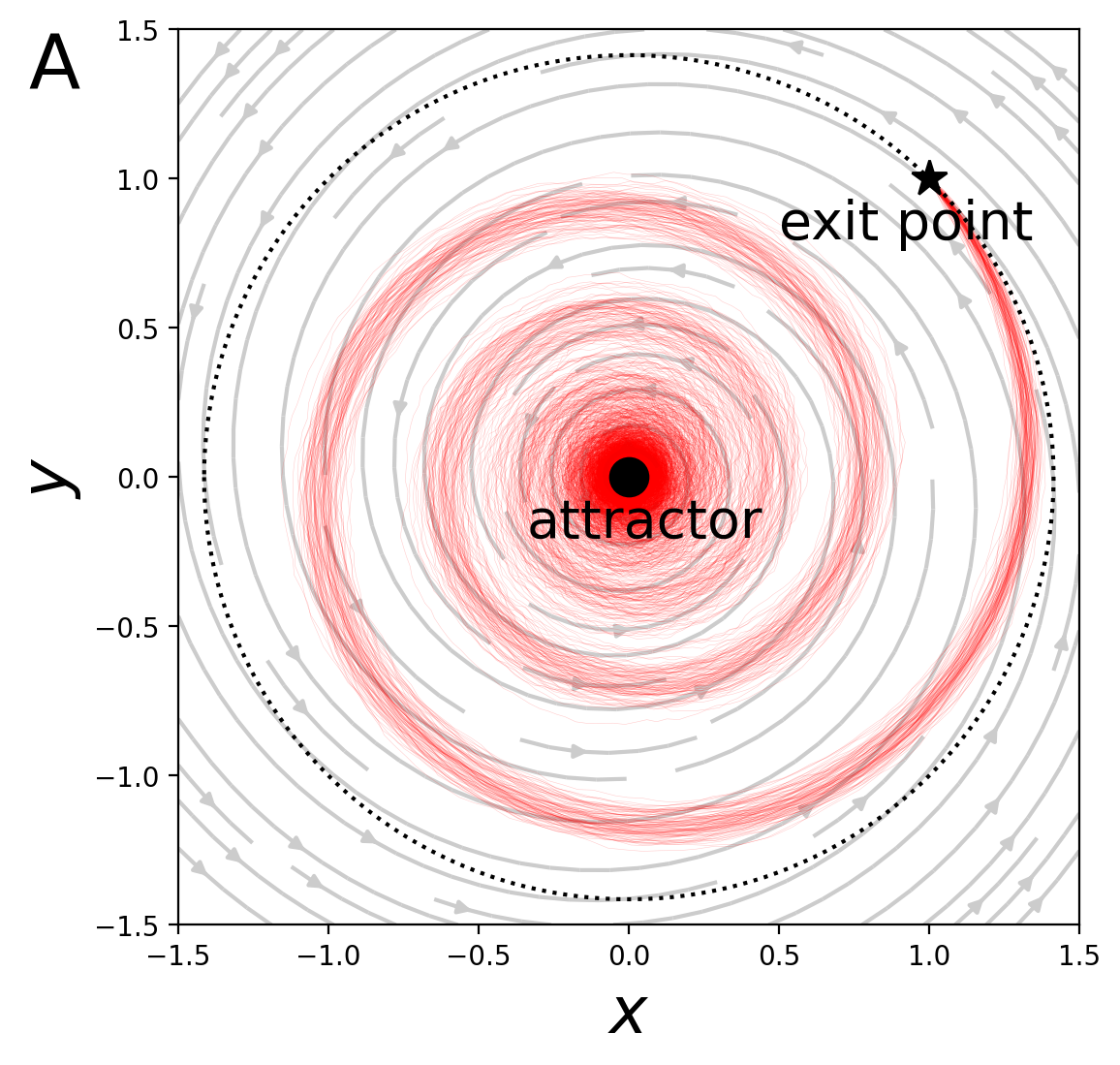
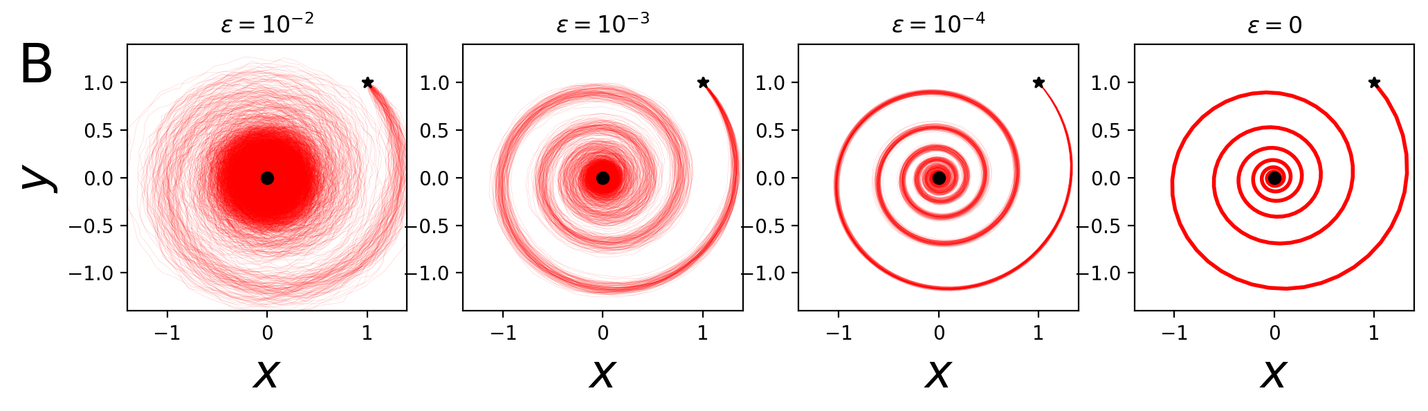
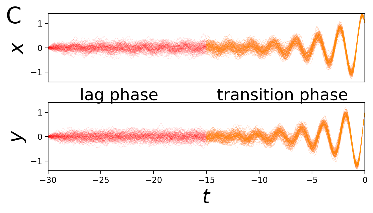
Figure 1: Single walker rare event. (A) Samples of the optimal escape trajectory (72) (red) for $\epsilon=10^{-3}$, with streamlines showing the deterministic flows ($\dot{x}=Ax$) for reference. (The optimal trajectory $T=\infty$ is approximated with $T=30$.) (B) The escape trajectories follow a "tube". As the noise magnitude $\epsilon$ goes to zero, the width of the "tube" goes to zero. (C) sampled conditional transition paths with $\epsilon=5\times 10^{-3}$ are shown as functions of time. The paths are separated into two segments or phases. The lag phase is shown as red and the transition phase is shown as orange. Other parameters are $\mu=0.25$, $\omega=3$.

To illustrate the exit trajectories, we focus on a single exit point $L=(1,1)$, but we note that any of the points on the circle $\|L\|=\text{const}$ (dashed line in Fig. 1A) are equally likely.

Several samples of conditional transition trajectories (72) are shown in Fig. 1. As the noise amplitude is decreased, the sampled trajectories condense into a tube like path, the center of which is the MLT (61). Several sample conditional paths are shown in Fig. 1C illustrating the two phases of a given rare event path: the exponentially long lag phase (shown in red) and the transition phase (shown in orange). Note that in general, the lag phase is likely to be much longer than shown.

Recall that we assume the distinguished limit $\epsilon\to 0$, $N\to\infty$ with $\epsilon\log(N)=\Lambda$. In regime 1, there is a labor shortage. If $\Lambda<V(L)$ then there are not enough walkers to overcome the exponentially long (in $\epsilon^{-1}$) lag phase (see Fig. 1C) and $\mathbb{E}[\tau^{N}_{\rm first}]\to\infty$ as $\epsilon\to 0$. The MLT is essentially described by the globally optimal $T\to\infty$ MLT (64) (see Fig. 1A,B). Increasing the number of walkers in this regime has the strongest effect on reducing the extreme first hitting time; that is, $\mathbb{E}[\tau^{N}_{\rm first}]\propto N^{-1}$. One can define a critical labor supply,

$$N_{*}=\exp(V(L)/\epsilon)=\exp\left(\frac{\mu}{2\epsilon}\|L\|^{2}\right),$$

which serves as a boundary between the regime 1 and 2.

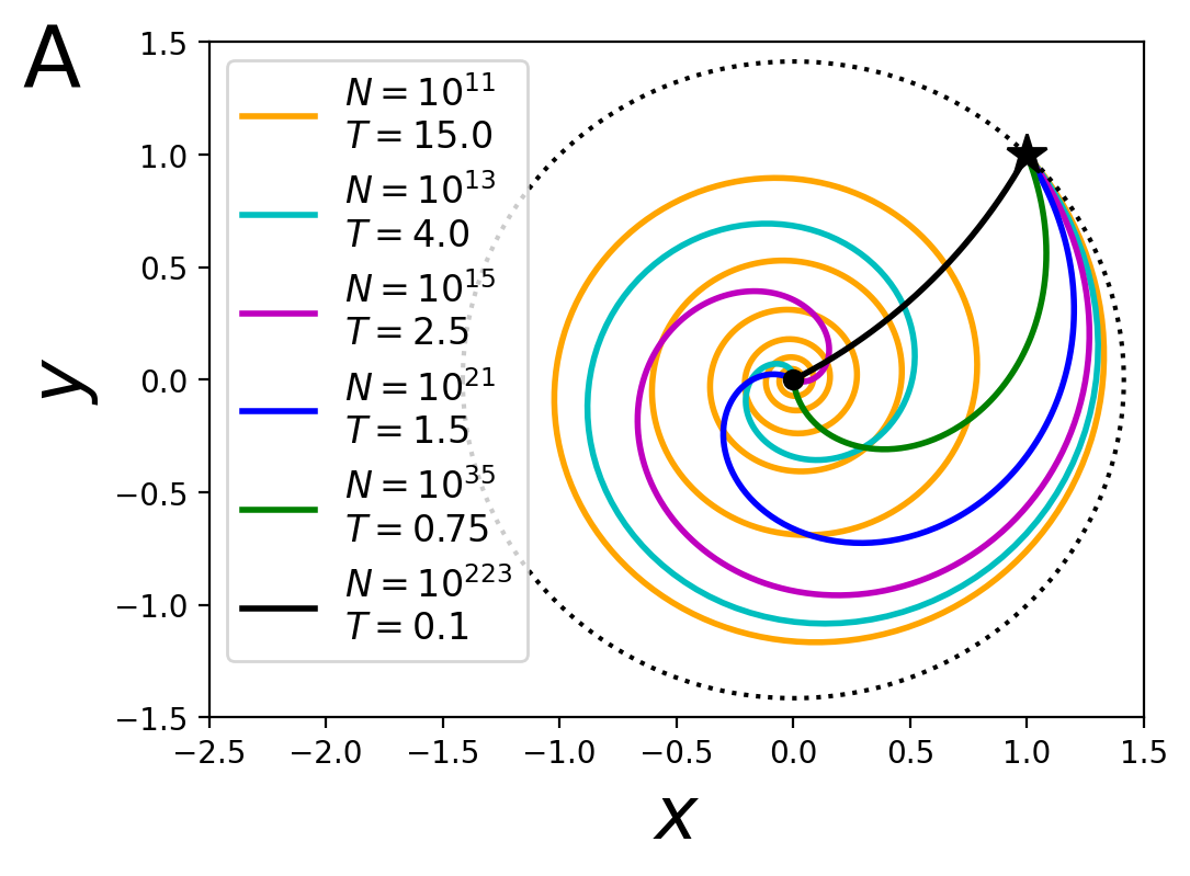
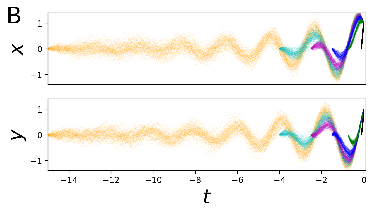
Figure 2: Trajectories in regime 2: balanced labor. In Regime 2, the MLTs are deformed as $N$ is increased ($T$ is decreased), with $N=\exp(S_{T|T}/\epsilon)$, $\epsilon=10^{-2}$. (A) Multiple suboptimal MLTs conditioned on the final time $T$. (B) Sampled transition paths for $\epsilon=10^{-2}$. For comparison, the trajectories are aligned at the end and shown backward in time. Other parameters are $\mu=0.25$, $\omega=3$.

In regime 2, the labor supply is balanced against the single-walker rare event time $\tau$. If $V(L)<\Lambda<S_{T|T}<\infty$ then $N>N_{*}$ and there is a sufficient number of walkers to accomplish the rare event in finite time as $\epsilon\to 0^{+}$. The MLT duration $T$ is finite and does not follow the same path as the globally optimal MLT. We have that $\mathbb{E}[\tau^{N}_{\rm first}]\sim T=\Psi_{L}(\Lambda)$, where $\Psi_{L}(\Lambda)$ is given by (16). The conditional mean $\varphi_{t|T}$ (61) is plotted in Fig. 2A for several values of $N$ (We also note the corresponding value of $T$). Sample paths are shown in Fig. 2B as functions of time. Increasing the number of walkers is equivalent to reducing $T$, which results in an MLT that moves more directly toward the exit point $L$. For exceedingly large $N$ (e.g., $N=10^{223}$ or equivalently $T=0.1$), the path is nearly a straight line (see the black curves in Fig. 2).

In regime 3, there is a labor surplus. As $\Lambda\to\infty$ we reach a regime where adding more walkers has the smallest effect on the extreme first hitting time; namely $\mathbb{E}[\tau^{N}_{\rm first}]\propto 1/\log(N)$. One way we could have the limit $\Lambda\to\infty$ is taking $N\to\infty$ with $\epsilon$ fixed. We know that we have a labor surplus when the cost function begins to scale like $S_{T|T}\sim MT^{-1}$, as $T\to 0^{+}$, for some constant $M>0$. The small $T$ asymptotics of the cost function has been studied for a large class of nonlinear SDEs [5, Ch. 11, p. 407], and it is known that the constant $M$ depends on the Riemannian length between the origin and $L$. With this scaling, we have that $\mathbb{E}[\tau^{N}_{\rm first}]=T\sim\frac{M}{\epsilon\log(N)}$, as $T\to 0^{+}$. We therefore conclude that the crossover timescale can be determine by the precise small $T$ asymptotics of $S_{T|T}$. In our simple example, expanding (63) around $T=0$ yields

$$S_{T|T}\sim\frac{\|L\|^{2}}{4}\left(T^{-1}+\mu+O(T)\right),\quad T\to 0^{+}.$$ (74)

Notice that the leading order term is independent of $\mu$ and $\omega$. The above expansion suggests that the crossover timescale is $T\ll 1/\mu$ which in turn identifies,

$$N>N_{**}=\exp\left(\frac{V(L,\mu^{-1})}{\epsilon}\right)$$ (75)

where the scaling of the extreme hitting time is $1/\log(N)$. The factor $M/\epsilon=\|L\|^{2}/(4\epsilon)$ is the mean first passage time for a single Brownian walker to reach the boundary of the circle of radius $L$, starting from the center. It is this time that is reduced by a factor of $1/\log(N)$ as $N\to\infty$ so that

$$\mathbb{E}[\tau^{N}_{\rm first}]\sim\frac{\left(\frac{\|L\|^{2}}{4\epsilon}\right)}{\log(N)},\quad N\to\infty.$$ (76)

5 Discussion

Our results start with the establishment of a connection between the number of walkers, $N$, and the duration of the MLT, $T$. This means that adding more walkers is equivalent to conditioning on a faster MLT. It has long been known in the Large Deviation Theory literature that, given a fixed exit point, the globally optimal MLT is given by $T\to\infty$, and it is these paths that determine the asymptotics of the single walker mean exit time. Hence, the $T\to\infty$ MLTs have received the most attention in the literature. By establishing a link between $N$ and $T$, we have identified a new application for the sub-optimal, finite $T$, MLTs.

The example in Section 4 involved a linear SDE. For general nonlinear problems, the best course of action is to employ numerical methods [10, 3, 27] and dynamical systems techniques [20, 21, 22, 27] to study the problem. The deterministic ($\epsilon=0$) dynamics should be studied first. The stochastic dynamics can then be understood through (17). Notable features that can occur in general nonlinear problems include the possibility that optimal ($T\to\infty$) MLTs are not unique [21, 27] and the behavior of MLTs near unstable critical points of the deterministic dynamics [22, 27]— particularly saddles, which often serve as boundaries between basins of attraction.

Finally, we note that our choice of using a continuous Markov process is purely for the sake of brevity. The theory of large deviations, including the characterization of rare events in terms of MLTs, has been extended to many other types of Markov process, including continuous time jump processes [5], piece-wise deterministic Markov processes [5, 26, 2], mixtures [27, 25, 35], and spatially extended Markov processes [4]. We emphasize that the results presented here should be generalized by applying LDT directly to the full process in question and not by employing an intermediate diffusion approximation. This is particularly true for the case where fast variables are averaged out [5, ch. 7], since this constrains the resulting MLT and leads to a characterization of the rare event using suboptimal trajectories [29, 28, 24]. A general strategy for applying a large deviation analysis to a given weak-noise Markov process is to start by calculating the Hamiltonian function analogous to Eqn. (10). The most straightforward way to accomplish this is with a WKB expansion [27]. Once the Hamiltonian is known, one can utilize numerical methods to solve the Hamilton-Jacobi equation (14) via (17).

Appendix A Appendix

We provide some extra details on the Ornstein-Uhlenbeck process of Section 4. It is well-known that $X_{t}$ is Gaussian [11, Section 5.6], and hence one can immediately infer that, writing $B_{\delta}(L)\subset\mathbb{R}^{2}$ to be a closed ball of radius $\delta$ about $L$,

$$\epsilon\log\mathbb{P}\big{(}x_{t}\in B_{\delta}(L)\big{)}=-\frac{1}{4}L^{T}U_{tt}^{-1}L+o(\epsilon,\delta),$$ (77)

where the corrections terms are negligible in taking $\epsilon\to 0^{+}$ (first), and then $\delta\to 0^{+}$ (second). We now claim that the above quadratic form is in fact the cost-function, and that the solution of (59) - (60) is in fact just the conditional mean (defined just below in (78).

To see this, for any $s\in[0,t]$, define $m_{s|t}\in\mathbb{R}^{2}$ to be the conditional mean, that is

$$m_{s|t} =\mathbb{E}\left[x_{s}\mid x_{t}=L,\,x_{0}=0\right]$$ (78)

$$=U_{st}U_{tt}^{-1}L$$ (79)

In fact one easily checks that both $m_{s|t}$ and $U_{rs|t}$ are independent of $\epsilon$.

Next, we claim that the cost-function assumes the form (for any $L\in\mathbb{R}^{2}$ and any $t>0$)

$$V(L,t)=\frac{1}{2}L^{T}U_{tt}^{-1}L.$$ (80)

To see why this holds, for any finite subset $\pi\subset[0,t]$, define the event

$$\mathcal{A}_{\pi,\tilde{\delta}}=\big{\{}y\in\mathcal{C}([0,t],\mathbb{R}^{2}),\;\sup_{s\in\pi}\|y_{s}-m_{s|t}\|\geq\tilde{\delta}\big{\}}$$ (81)

We can thus conclude that for any $\tilde{\delta}>0$,

$$\underset{\delta\to 0}{\overline{\lim}}\underset{\epsilon\to 0}{\overline{\lim}}\epsilon\log\mathbb{P}\big{(}x_{t}\in B_{\delta}(L)\big{)}-\underset{\delta\to 0}{\overline{\lim}}\underset{\epsilon\to 0}{\overline{\lim}}\epsilon\log\mathbb{P}\big{(}x_{t}\in B_{\delta}(L),x\in\mathcal{A}_{\pi,\tilde{\delta}}\big{)}\\ =\frac{1}{2}\sup_{y\in\mathcal{A}_{\pi,\tilde{\delta}}}\sum_{r,s\in\pi}\sum_{a,b\in\{1,2\}}y_{r}(a)y_{s}(b)\tilde{V}_{rs}(a,b)>0$$ (82)

where $\tilde{V}=\big{(}\tilde{V}_{rs}(a,b)\big{)}_{r,s\in\pi,a,b\in\{1,2\}}\in\mathbb{R}^{2|\pi|\times 2|\pi|}$ is the covariance matrix with elements $\big{(}U_{rs|t}(a,b)\big{)}_{r,s\in\pi,a,b\in\{1,2\}}$. Indeed the RHS of (82) is strictly positive because $\tilde{V}$ must be strictly positive definite (the inverse of a positive definite symmetric matrix is codiagonal with the original matrix, with each eigenvalues the inverse of one of the original eigenvalues).

It follows from (82) that

$$\lim_{\delta\to 0^{+}}\lim_{\epsilon\to 0^{+}}\epsilon\log\mathbb{P}\big{(}x_{t}\in B_{\delta}(L)\big{)}=\lim_{\delta\to 0^{+}}\lim_{\epsilon\to 0^{+}}\epsilon\log\mathbb{P}\big{(}\sup_{s\in[0,t]}\|x_{s}-\phi_{s|t}\|\leq\delta\big{)}.$$ (83)

Because the Large Deviations Rate Function $I_{T}$ is lower-semi-continuous, this implies that

$$\inf_{z\in H_{1}\;:z_{t}=L}I_{T}(z)=I_{T}(\phi)$$ (84)

which immediately implies (80).

It is also known that [11] the covariance matrix satisfies the ODE

$$\frac{d}{dt}U_{tt} =AU_{tt}+U_{tt}A^{T}+2\mathbb{I}$$ (85)

$$U_{00} =0\mathbb{I}.$$ (86)

Because the eigenvalues of $A$ have negative real parts, there must exist a unique invariant distribution to the stochastic dynamics (54). This distribution is centered and Gaussian, with covariance matrix $U_{*}\in\mathbb{R}^{2\times 2}$ satisfying the identity

$$AU_{*}+U_{*}A^{T}+2\mathbb{I}=0.$$ (87)

That is, there is a unique positive-definite symmetric matrix $U_{*}$ satisfying the above identity, and $U_{tt}$ converges to $U_{*}$ as $t\to\infty$. We thus find that the quasi-potential is

$$V(L)=\frac{1}{2}L^{T}U_{*}^{-1}L.$$ (88)

References

- [1] Alan J Bray, Satya N Majumdar, and Grégory Schehr. Persistence and first-passage properties in nonequilibrium systems. Advances in Physics, 62(3):225–361, 2013.
- [2] Paul C Bressloff and Jay M Newby. Path integrals and large deviations in stochastic hybrid systems. Physical Review E, 89(4):042701, 2014.
- [3] MK Cameron. Finding the quasipotential for nongradient sdes. Physica D: Nonlinear Phenomena, 241(18):1532–1550, 2012.
- [4] Amir Dembo and Ofer Zeitouni. Large deviations techniques and applications. Second Edition, volume 38. Springer Science & Business Media, 2009.
- [5] Mark I Freidlin and Alexander D Wentzell. Random Perturbations of Dynamical Systems, volume 260. Springer Science & Business Media, 2012.
- [6] Mark Iosifovich Freidlin, Alexander D Wentzell, MI Freidlin, and AD Wentzell. Random perturbations. Springer, 1998.
- [7] Crispin Gardiner. Stochastic methods, volume 4. Springer Berlin, 2009.
- [8] Tobias Grafke and Eric Vanden-Eijnden. Numerical computation of rare events via large deviation theory. Chaos: An Interdisciplinary Journal of Nonlinear Science, 29(6):063118, 2019.
- [9] Magnus J Haughey, Aleix Bassolas, Sandro Sousa, Ann-Marie Baker, Trevor A Graham, Vincenzo Nicosia, and Weini Huang. First passage time analysis of spatial mutation patterns reveals sub-clonal evolutionary dynamics in colorectal cancer. PLOS Computational Biology, 19(3):e1010952, 2023.
- [10] Matthias Heymann and Eric Vanden-Eijnden. The geometric minimum action method: A least action principle on the space of curves. Communications on Pure and Applied Mathematics: A Journal Issued by the Courant Institute of Mathematical Sciences, 61(8):1052–1117, 2008.
- [11] Ioannis Karatzas, Steven E Shreve, Ioannis Karatzas, and Steven E Shreve. Brownian motion. Brownian motion and stochastic calculus, pages 47–127, 1998.
- [12] Joseph B Keller. Diffusion at finite speed and random walks. Proceedings of the National Academy of Sciences, 101(5):1120–1122, 2004.
- [13] Venu Kurella, Justin C Tzou, Daniel Coombs, and Michael J Ward. Asymptotic analysis of first passage time problems inspired by ecology. Bulletin of mathematical biology, 77(1):83–125, 2015.
- [14] Sean D Lawley. Distribution of extreme first passage times of diffusion. Journal of Mathematical Biology, 80(7):2301–2325, 2020.
- [15] Sean D Lawley and Jacob B Madrid. A probabilistic approach to extreme statistics of brownian escape times in dimensions 1, 2, and 3. Journal of Nonlinear Science, 30(3):1207–1227, 2020.
- [16] Georg Lindgren, Holger Rootzén, and Maria Sandsten. Stationary stochastic processes for scientists and engineers. CRC press, 2013.
- [17] Samantha Linn and Sean D Lawley. Extreme hitting probabilities for diffusion. Journal of Physics A: Mathematical and Theoretical, 55(34), 2022.
- [18] Donald Ludwig. Persistence of dynamical systems under random perturbations. Siam Review, 17(4):605–640, 1975.
- [19] Jacob B Madrid and Sean D Lawley. Competition between slow and fast regimes for extreme first passage times of diffusion. Journal of Physics A: Mathematical and Theoretical, 53(33):335002, 2020.
- [20] Robert S Maier and Daniel L Stein. Escape problem for irreversible systems. Physical Review E, 48(2):931, 1993.
- [21] Robert S Maier and Daniel L Stein. A scaling theory of bifurcations in the symmetric weak-noise escape problem. Journal of statistical physics, 83:291–357, 1996.
- [22] Robert S Maier and Daniel L Stein. Limiting exit location distributions in the stochastic exit problem. SIAM Journal on Applied Mathematics, 57(3):752–790, 1997.
- [23] Victor Matveev. Comparison of deterministic and stochastic approaches for calcium dependent exocytosis. Biophysical Journal, 114(3):283a–284a, 2018.
- [24] J Newby and J Chapman. Metastable behavior in markov processes with internal states: breakdown of model reduction techniques. J. Math. Biol., 10, 2013.
- [25] Jay Newby. Bistable switching asymptotics for the self regulating gene. Journal of Physics A: Mathematical and Theoretical, 48(18):185001, 2015.
- [26] Jay M Newby. Isolating intrinsic noise sources in a stochastic genetic switch. Physical biology, 9(2):026002, 2012.
- [27] Jay M Newby. Spontaneous excitability in the morris–lecar model with ion channel noise. SIAM Journal on Applied Dynamical Systems, 13(4):1756–1791, 2014.
- [28] Jay M Newby, Paul C Bressloff, and James P Keener. Breakdown of fast-slow analysis in an excitable system with channel noise. Physical Review Letters, 111:128121, 2013.
- [29] Jay M Newby and James P Keener. An asymptotic analysis of the spatially inhomogeneous velocity-jump process. Multiscale Modeling & Simulation, 9(2):735–765, 2011.
- [30] Lukas Ramlow, Martin Falcke, and Benjamin Lindner. An integrate-and-fire approach to ca2+ signaling. part i: Renewal model. Biophysical Journal, 122(4):713–736, 2023.
- [31] Jürgen Reingruber and David Holcman. Computational and mathematical methods for morphogenetic gradient analysis, boundary formation and axonal targeting. Seminars in Cell & Developmental Biology, 35:189–202, 2014. Regulated Necrosis & Modeling developmental signaling pathways & Development of connective maps in the brain.
- [32] Z Schuss, K Basnayake, and D Holcman. Redundancy principle and the role of extreme statistics in molecular and cellular biology. Physics of life reviews, 28:52–79, 2019.
- [33] Gregory D Smith, Joel E Keizer, Michael D Stern, W Jonathan Lederer, and Heping Cheng. A simple numerical model of calcium spark formation and detection in cardiac myocytes. Biophysical journal, 75(1):15–32, 1998.
- [34] Srinivasa RS Varadhan. Diffusion processes in a small time interval. Communications on Pure and Applied Mathematics, 20(4):659–685, 1967.
- [35] Benjamin L Walker and Katherine A Newhall. Numerical computation of effective thermal equilibria in stochastically switching langevin systems. Physical Review E, 105(6):064113, 2022.
- [36] George H. Weiss and Menachem Dishon. On the asymptotic behavior of the stochastic and deterministic models of an epidemic. Mathematical Biosciences, 11(3):261–265, 1971.
- [37] George H Weiss, Kurt E Shuler, and Katja Lindenberg. Order statistics for first passage times in diffusion processes. Journal of Statistical Physics, 31:255–278, 1983.