Effective Hamiltonian approach to the kinetic infinitely long-range Ising (the Husimi-Temperley) model

Abstract

The linear master equation (ME) describing the stochastic kinetics of Ising-type models has been transformed into a nonlinear ME (NLME) for a time-dependent effective Hamiltonian (EH). It has been argued that for models with large number of spins ($N$) NLME is easier to deal with numerically than ME. The reason is that the non-equilibrium probability distribution entering ME scales exponentially with the system size which for large $N$ causes numerical under- and overflow problems. NLME, in contrast, contains quantities scaling with $N$ not faster than linearly.

The advantages of NLME in numerical calculations has been illustrated on the problem of decay of metastable states in the kinetic Husimi-Temperley model (HTM) previously studied within ME approach by other authors. It has been shown that the use of NLME makes possible to extend by orders of magnitude the ranges of numerically accessible quantities, such as the system size $N$ and the lifetimes of metastable states, as well as the accuracy of the calculations. An excellent agreement of numerical results with previous studies has been found.

It has been shown that in the thermodynamic limit EH for HTM exactly satisfies a nonlinear first order differential equation. The system of characteristic equations for its solution has been derived and it has been shown that the conventional mean field equation is one of them.

I Introduction

The equilibrium statistics of a classical many-body system at a fixed temperature can be described by the canonical probability distribution (CPD) [1]. In this paper we will deal with the spin-lattice models frequently used to describe statistics of uniaxial magnets, lattice gases, and binary alloys [1, 2, 3]. In these models CPD depends only on the configuration energy which is conventionally called the Hamiltonian. The CPD is proportional to the Boltzmann factor which is the exponential function of the Hamiltonian divided by $-k_{B}T$—the absolute temperature in energy units with the minus sign [1]. In models with short-range interactions the energy scales linearly with the system size $N$. So if exact analytic solution is unknown, the straightforward use of CPD in approximate calculations would necessitate numerical calculation of the exponential function with the argument scaling as $O(N)$ which can be difficult or even impossible for large $N$. To deal with this problem sophisticated combinatorial techniques have been developed to make possible the calculation of quantities of interest without resorting to the numerical exponentiation and using only $O(1)$ quantities, such as the specific magnetization and the energy density per site [1].

From the standpoint of out of equilibrium statistics CPD is a particular case of more general non-equilibrium probability distribution (NPD) which coincides with CPD in thermal equilibrium. This is conveniently formalized in the effective Hamiltonian (EH) approach [4, 5, 6] where the dependence of NPD on EH is posited to be the same as that of CPD on the equilibrium Hamiltonian. This is achieved by defining EH as the logarithm of NPD multiplied by $-k_{B}T$. This trick allows one to use the approximate techniques of equilibrium statistics [1] also in the non-equilibrium case.

This, however, does not fully solve the problem because unlike the equilibrium case where the Hamiltonian is constant and is supposed to be known, when the system is out of equilibrium EH should be determined separately. In the case of the kinetic Ising models [7, 8, 9], EH evolves with time according to the master equation (ME) for NPD [7]. Because NPD depends on EH and $N$ exponentially, the numerical solution of ME for large $N$ encounters the same over- and underflow difficulties as in the statistical averaging.

The aim of the present paper is to suggest a modification of ME along the lines of Ref. [4] such that in the case of homogeneous systems with short range interactions the resulting evolution equation contained only quantities $O(1)$. It will be shown that this can be achieved at the cost of transforming the linear ME into a nonlinear evolution equation which will be abbreviated as NLME. Its derivation will be given in Sec. II. NLME for the kinetic Husimi-Temperley model (HTM) (also known as the infinitely long-range Ising-, the mean field- (MF), the Curie-Weiss-, and the Weiss-Ising model [10, 11, 12, 13, 14]) evolving under the Glauber dynamics [8] will be derived in Sec. III. The advantages of NLME will be illustrated on the problem of decay of metastable states in HTM. The decay problem was previously investigated in Refs. [10, 11, 13] in the framework of ME, the Fokker-Planck equation, and the Monte Carlo simulations. A scaling law for the lifetime of metastable states was suggested and shown to be valid for large absolute values of a scaling parameter [13]. In Secs. IV and VI it will be shown that the use of NLME allows one to extend the testing range of the scaling law as well as the accuracy of the calculated lifetimes of the metastable states by orders of magnitude. Finally, In Sec. V it will be shown that NLME for HTM in the thermodynamic limit reduces to a nonlinear differential equation of the first order. The characteristic equations will be derived and it will be shown that the conventional MF kinetic equation of Refs. [15, 12, 3] describes a characteristic passing through the minimum of a free energy function. In concluding Sec. VII a brief summary will be presented and further arguments given to support the suggestion that NLME is a prospective approach to the solution of stochastic models of the Ising type.

II Effective Hamiltonian approach to the kinetic Ising models

For brevity, the set of $N$ Ising spins $\sigma_{i}=\pm 1$, $i=1,N$, will be denoted as $\pmb{\sigma}=\{\sigma_{i}\}$. In the stochastic approach to non-equilibrium kinetics the statistical properties of an out of equilibrium system can be described by the time-dependent NPD $P(\pmb{\sigma},t)$ which satisfies the ME [7]

$${P}_{t}(\pmb{\sigma},t)=\sum_{\pmb{\sigma}^{\prime}}[r(\pmb{\sigma}^{\prime}\to\pmb{\sigma},t)P(\pmb{\sigma}^{\prime},t)-r(\pmb{\sigma}\to\pmb{\sigma}^{\prime},t).P(\pmb{\sigma},t)],$$ (1)

Here and in the following by subscript $t$ we will denote the partial time derivative; the transition rates $r$ in the kinetic Ising models will be chosen according to Refs. [8, 9] as

$$r(\pmb{\sigma}\to\pmb{\sigma}^{\prime},t)=\frac{1}{\tau_{0}}\frac{e^{{-\cal H}^{0}(\pmb{\sigma}^{\prime},t)}}{e^{-{\cal H}^{0}(\pmb{\sigma}^{\prime},t)}+e^{-{\cal H}^{0}(\pmb{\sigma},t)}}.$$ (2)

where $1/\tau_{0}$ is the rate of transition $\pmb{\sigma}\to\pmb{\sigma}^{\prime}$ and the dimensionless Hamiltonian ${\cal H}^{0}$ is assumed to include the Boltzmann factor $\beta=1/k_{B}T$ as one of the parameters. ${\cal H}^{0}$ may depend on time which is necessary, for example, in modeling hysteretic phenomena [12]. The dependence of the Hamiltonian on $\pmb{\sigma}$ can be arbitrary but in this study we will assume that ${\cal H}^{0}$ is an extensive quantity, that is, it scales linearly with the system size $N$ [1]. In this case the exponential functions in Eq. (2) scale with $N$ as

$$e^{-{\cal H}^{0}(\pmb{\sigma},t)}=e^{-u^{0}(\pmb{\sigma},t)N},$$ (3)

where $u^{0}=O(1)$ is the Hamiltonian density. The exponential behavior in Eq. (3) may hinder numerical solution of ME (1) because the terms on the right hand side (rhs) of Eq. (2) will suffer from the problem of numerical over- and underflow at sufficiently large $N$. However, when the transition $\pmb{\sigma}\to\pmb{\sigma}^{\prime}$ is local, this difficulty is easily overcome. Multiplying the numerator and denominator in Eq. (2) by $\exp\{\tfrac{1}{2}[{\cal H}^{0}(\pmb{\sigma},t)+{\cal H}^{0}(\pmb{\sigma}^{\prime},t)]\}$ one arrives at

$$r(\pmb{\sigma}\to\pmb{\sigma}^{\prime})=\frac{1}{2\tau_{0}}\frac{\exp{[\tfrac{1}{2}\Delta^{{\cal H}^{0}}(\pmb{\sigma},\pmb{\sigma}^{\prime},t)}]}{\cosh[{\tfrac{1}{2}\Delta^{{\cal H}^{0}}(\pmb{\sigma},\pmb{\sigma}^{\prime},t)}]}$$ (4)

where

$$\Delta^{{\cal H}^{0}}(\pmb{\sigma},\pmb{\sigma}^{\prime},t)={\cal H}^{0}(\pmb{\sigma},t)-{\cal H}^{0}(\pmb{\sigma}^{\prime},t).$$ (5)

In lattice models with local spin interactions the $O(N)$ scaling of ${\cal H}^{0}$ is a consequence of the summation over $N$ lattice sites. If configurations $\pmb{\sigma}$ and $\pmb{\sigma}^{\prime}$ differ only locally, the difference in Eq. (5) in such models vanishes at large distances from the region of the flipping spins so the summations over sites will be spatially restricted leading to $\Delta^{{\cal H}^{0}}=O(1)$, hence, all terms in Eq. (4) will be of order unity.

We note that Eq. (5) is antisymmetric under the exchange of spin arguments so the denominator in Eq. (4) is the same for both terms in Eq. (1). Replacing it by a constant can simplify ME while preserving its qualitative features [4, 12]. In the present paper, however, more complex Glauber prescription (2) will be used for compatibility with the majority of literature on the kinetic HTM (see, e.g., Refs. [16, 13] and references therein).

Another source of the undesirable behavior briefly discussed in the Introduction comes from NPD $P$ which should depend on $N$ similar to CPD because it would coincide with it in thermal equilibrium

$$P(\pmb{\sigma},t)|_{t\to\infty}\to P^{0}(\pmb{\sigma})=e^{-{\cal H}^{0}(\pmb{\sigma})}/Z$$ (6)

where $Z$ is the partition function and ${\cal H}^{0}$ in Eq. (6) is assumed to be time-independent because otherwise the equilibrium would not be attainable. It is easily checked that $P^{0}$ is a stationary solution of Eq. (1) which means that at least for large $t$ NPD $P$ in Eq. (1) behaves similar to $P^{0}$. This can be formalized in the EH approach [4, 6, 3] where by analogy with Eqs. (6) and (3) NPD is depends on EH ${\cal H}$ as

$$P(\pmb{\sigma},t)=e^{-{\cal H}(\pmb{\sigma},t)}\equiv e^{-Nu(\pmb{\sigma},t)},$$ (7)

where ${\cal H}|_{t\to\infty}\to{\cal H}^{0}+\ln Z$ and $u$ is the EH density. In Eq. (7) it has been assumed that the normalization constant similar to $\ln Z$ is included in ${\cal H}$. This is convenient in many cases because ME (1) preserves normalization so whenever possible the initial ${\cal H}(\pmb{\sigma},t=t_{0})$ is reasonable to choose in such a way that $P(t_{0})$ in Eq. (7) was easily normalizable. This would eliminate the necessity to calculate an equivalent of the partition function $Z$ at later stages of evolution because in general this is a nontrivial task.

In Ref. [4] a simple way to eliminate the undesirable exponential behavior from ME is suggested which was implemented as follows. Dividing both sides of Eq. (1) by $P$ from Eq. (7) one arrives after trivial rearrangement at the evolution equation for EH

$${\cal H}_{t}(\pmb{\sigma},t)=\sum_{\pmb{\sigma}^{\prime}}\frac{\exp\left(-\tfrac{1}{2}\Delta^{{\cal H}^{0}}\right)-\exp\left(\tfrac{1}{2}\Delta^{{\cal H}^{0}}-\Delta^{{\cal H}}\right)}{2\tau_{0}\cosh(\tfrac{1}{2}\Delta^{{\cal H}^{0}})}$$ (8)

where $\Delta^{\cal H}$ is defined as in Eq. (5) and by similar reasoning it should be an $O(1)$ quantity. The arguments of deltas in Eq. (8) have been omitted for brevity; they are the same as in Eq. (5). As is seen, all terms on the rhs are $O(1)$ but because of the summation over $\pmb{\sigma}^{\prime}$ the equation scales linearly with $N$.

However, if the system is spatially homogeneous, Eq. (8) can be further reduced to an $O(1)$ equation. For example, if the sites are organized in a Bravais lattice, all sites are equivalent and summations over sites implicit on both sites of the equation can be lifted. Presumably, this can be achieved with the use of the formalism developed in the cluster approach to equilibrium alloy theory [2]. In this approach Eq. (8) should be formally expanded over a complete set of orthonormal polynomial functions of $\pmb{\sigma}$ characterized by the clusters of lattice sites of all possible configurations and positions [17]. The total number of the basis functions is exponentially large ($\sim 2^{N}$) but in the spatially homogeneous case the coefficients of clusters differing only by their position on the lattice will be the same. Therefore, only clusters in the vicinity of a single lattice site need be taken into account. Further, if the interactions in the system are local, i.e., cluster sizes are bounded by a maximum radius, the size of the system of equations can also be bounded. In practice in the alloy thermodynamics the number of clusters to keep in the expansion was found to be rather moderate in many cases [18, 19]. Hopefully, similarly simple approximations will be possible to develop in the non-equilibrium statistics as well. This case, however, is more difficult because in the EH long range interactions may arise due to kinetics [4].

III Application to HTM

The HTM is an Ising-type model in which all spin pairs interact with the same strength $J/N$ so the dimensionless Hamiltonian can be express in terms of the total spin [13]

$$M=\sum_{i=1}^{N}\sigma_{i}\equiv Nm$$ (9)

as

$${\cal H}^{0} = -\frac{\beta J}{2}M^{2}-\beta{H(t)}M$$ (10)

$$= -N\left[\frac{\beta}{2}m^{2}-h(t)m\right]\equiv Nu^{0}(m,t),$$

where $m=O(1)$ is the specific magnetization and to simplify notation we have chosen $J$ as our energy unit $J=1$ so that the HTM critical temperature will satisfy $k_{B}T_{c}=\beta_{c}^{-1}=1$; $h(t)=\beta H(t)$ is the external magnetic field which can depend on time, though in the present study we will be interested mainly in constant-$h$ case. In Eq. (10) $u^{0}(m,t)$ is the physical Hamiltonian density which we will distinguish from the equilibrium Hamiltonian density because the equilibrium is incompatible with the time-dependence.

The physical picture is easier visualized in terms of function [13]

$$f^{0}(m,t)=u^{0}(m,t)-s(m)$$ (11)

where

$$s(m)=-\sum_{\genfrac{(}{)}{0.0pt}{2}{up}{lo}}\frac{1\pm m}{2}\ln\frac{1\pm m}{2}$$ (12)

is the dimensionless entropy in the Stirling approximation. We will call $f^{0}$ the fluctuating free energy (FFE) because unlike the true free energy it is not convex. A typical FFE for HTM that will be studied below is shown in Fig. 1.

Figure 1: Equilibrium FFE Eq. (11) for $T=0.8T_{c}$ and $h=0.015$. A, B, and C denote, respectively, the two local minima and a local maximum appearing in $f^{0}(m)$ when $T<T_{c}$ and $|h|<|h_{SP}|$ where $h_{SP}$ is $h$ at the spinodal point (further explanations are given in the text).

$h_{SP}$ in Fig. 1 and magnetization $m_{SP}$ below in Eq. (45) are the values of $h$ and $m$ at the spinodal point defined by conditions

$$f^{0}_{m}=0\mbox{\ and\ }f^{0}_{mm}=0.$$ (13)

The explicit expressions can be found in Ref. [13]. In Eq. (13) and in the following the subscript $m$ will denote the symmetric discrete derivative defined for an arbitrary function $g(m)$ as

$$g_{m}(m)=\frac{g(m+\epsilon)-g(m-\epsilon)}{2\epsilon},$$ (14)

where $\epsilon=1/N$. For example, from Eq. (10) one gets

$$u_{m}^{0}(m,t)=-\beta m-h(t).$$ (15)

III.1 NLME for HTM

The choice of the kinetic HTM for the present study has been motivated mainly by its simplicity but also because it has been extensively studied previously within the linear master- and the Fokker-Planck equation approach in Refs. [10, 11, 13]. Most pertinent to our study will be the numerical data of Ref. [13] so to facilitate comparison we will try to follow the notation of that paper.

NLME for HTM can be derived straightforwardly from Eq. (8) using explicit expression for the physical Hamiltonian Eq. (10). However, in order to facilitate comparison with Ref. [13], below we derive it departing from Eq. (7) of that reference. To this end we first note that in Ref. [13] the authors considered the probability distribution of the magnetization $M$ as the fluctuating quantity. We will denote it as $P^{(M)}$. Our $P$, however, describes the distribution of the fluctuating Ising spins; $M$ and $m$ in our formulas should be considered as a shorthand for the sum of spins Eq. (9). The configuration space in the latter case consists of $2^{N}$ points while $M$ takes only $N+1$ values from $-N$ to $N$ with step 2 (a spin flip changes $M$ by 2). This is because many spin configurations correspond to one $M$ value which can be accounted for by a combinatorial factor ${}_{N}C_{N_{\pm}}$

$$P^{(M)}(M,t)=\frac{N!}{N_{+}!N_{-}!}P(M,t),$$ (16)

where $N_{+}=(N+M)/2$ and $N_{-}=(N-M)/2$) are the numbers of, respectively, spins +1 and -1 in the configuration.

In our notation Eq. (7) of Ref. [13] reads

$$P^{(M)}_{t}(M,t)=-\frac{1}{2\tau_{0}}\sum_{\genfrac{(}{)}{0.0pt}{2}{up}{lo}}\left(N_{\pm}\frac{\exp[\mp\beta(M\mp 1)/N\mp h]}{\cosh[\beta(M\mp 1)/N+h]}P^{(M)}(M)-(N_{\mp}+1)\frac{\exp[\pm\beta(M\mp 1)/N\pm h]}{\cosh[\beta(M\mp 1)/N+h]}P^{(M)}(M\mp 2)\right),$$ (17)

where the time arguments on the right hand side have been omitted for brevity and the sum consists of two terms: one with all lower signs and the other one with all upper signs. It should be noted that one of the terms disappears at the end points $M=\pm N$ because $|M|>N$ is not allowed.

Now substituting Eqs. (16) and (7) into Eq. (17) one obtains NLME containing only intensive quantities :

$$u_{t}(m,t)=\frac{1}{4\tau_{0}}\sum_{\genfrac{(}{)}{0.0pt}{2}{up}{lo}}(1\pm m)\left(\frac{\exp[\pm u_{m}^{0}(m\mp\epsilon,t)]}{\cosh[u_{m}^{0}(m\mp\epsilon,t)]}-\frac{\exp[\mp u_{m}^{0}(m\mp\epsilon,t)]}{\cosh[u_{m}^{0}(m\mp\epsilon,t)]}e^{\pm 2u_{{m}}(m\mp\epsilon,t)}\right).$$ (18)

As expected, each term on the rhs of Eq. (18) turns to zero for $u_{m}(m,t)=u_{m}^{0}(m)$ which is a direct consequence of the detailed balance condition satisfied by $r$ in Eq. (2). An important observation is that Eq. (18) contains only derivatives of $u$ with respect to $t$ and $m$ so the constant contribution to EH do not change during the evolution which makes possible normalization of the solution either in the initial condition or at any time during the evolution. It should be noted that in the derivation no approximations have been made so Eq. (18) is exact.

IV Metastable state evolution

To test NLME in concrete calculations we have numerically simulated the decay of a metastable state in the vicinity of minimum A in Fig. 1 which was investigated in Ref. [13]. Following that study the initial condition has been chosen as the Gaussian distribution

$$P^{(M)}(Nm,t=0)=\sqrt{\frac{aN}{2\pi}}\exp\left[-\frac{aN}{2}(m-m_{A})^{2}\right].$$ (19)

The initial condition for $u$ needed in Eq. (18) is obtained from an approximate equation

$$P^{(M)}(M,t=0)\simeq e^{-Nf(m,t=0)}$$ (20)

where in complete analogy with Eq. (11)

$$f(m,t)=u(m,t)-s(m).$$ (21)

The approximation consists in using Strling’s formula for the combinatorial factor in Eq. (16). This is admissible in the case of sufficiently deep metastable minima that we are going to consider because the initial condition $u(m,t_{0})$ can be arbitrary so the slight difference with Ref. [13] is unimportant, as discussed in detail below.

In all calculations parameter $a$ in Eq. (19) has been fixed at the same arbitrarily chosen value $a=1$. Obviously that in general the initial value should strongly influence the outcome of the evolution. However, in our case this will not be significant for the following reason. As was pointed out in Refs. [10, 11, 13], the problem of decay of a metastable state in HTM is akin to the problem of escape over the potential barrier in a two-well potential studied by Kramers [20]. In Ref. [21] the decay is described as follows. At the first stage the arbitrary initial magnetization distribution (in our case) relaxes toward a local quasi-equilibrium state and on the second stage this state slowly (in comparison with the first stage) decays into the stable equilibrium with the magnetic momenta distributed mainly around point B in Fig. 1. In the present study the lifetime $\tau$ has been determined at this second stage in contrast to Ref. [13] where the first stage was also included. Because in our definition the properties of both the minima and the Glauber rates depend only on the parameters of HTM, lifetime $\tau$ does not depend on arbitrariness of the initial distribution. Specifically, similar to Ref. [13] it has been assumed that the probability to find the system at time $t$ in the state with negative magnetization satisfies the conventional exponential decay law

$$n_{A}(t)=\int_{-1}^{0}P^{(M)}(Nm,t)dm\simeq n_{A}^{0}e^{-t/\tau},$$ (22)

the difference being that in the present study the law has been assumed to hold only after the initial relaxation has completed while in Ref. [13] it was considered to be approximately valid throughout the whole decay process. In view of this difference, the comparison of our lifetime $\tau$ with the calculations of Ref. [13] would be legitimate only if the initial fast relaxation time is negligible in comparison with $\tau$. This has been achieved by restricting consideration to sufficiently deep potential wells near the local minimum A which can be easily satisfied in large systems $N\geq 1000$ where the depth of even a shallow well in $f^{0}$ in Fig. 1 is strongly enhanced by the factor $N$ in the expressions of the Arrhenius type satisfied by the lifetime [20, 10, 11, 13]

$$\tau\sim e^{N[f^{0}(C)-f^{0}(A)]}\equiv e^{N\Delta f^{0}}$$ (23)

(we remind that $\beta$ enters the definition of $f^{0}$).

The qualitative picture just described is illustrated in Fig. 2 where it can be seen that the decay law Eq. (22) is satisfied at least within twelve orders of magnitude. The influence of the initial relaxation could not be discerned at the time resolution $100\tau_{0}$. It is to be noted that the lifetime $\tau$ in Fig. 2 is the second smallest in all of our calculations so the influence of the initial relaxation in most of them has been even weaker.

Though the decay law Eq. (22) is only heuristic, in the calculations it has been satisfied with a remarkable accuracy. The specific decay rate

$$\lambda=\tau^{-1}/N$$ (24)

has been found to be equal to $5.550091955(7)\times 10^{-7}$ at $t=200\tau_{0},300\tau_{0},400\tau_{0},500\tau_{0},$ and $5\cdot 10^{4}\tau_{0}$, that is, it had the same value to the accuracy in nine to ten significant digits.

Figure 2: Probability of survival of the metastable states Eq. (22) calculated with the use of Eq. (18) for HTM with $N=10^{3}$, $T=0.8T_{c}$, and $h=0.06$. The points are spaced with time step $100\tau_{0}$ and their size exceeds the accuracy of calculations. The exponential law has been fulfilled better than the accuracy of the drawing (see the text).

The simplicity of the behavior seen in Fig. 2 suggests a simple underlying physics which can be surmised from the behavior of FFE during the decay shown in Fig. 3. As can be seen, at intermediate times ($t=500\tau_{0}$ has been chosen as an example) $f(m,t)$ in the vicinity of local minima A and B in Fig. 1 can be accurately approximated as

$$f(m,t)\approx f^{0}(m)+C_{A(B)}(t).$$ (25)

In terms of NPD this translates into two quasi-equilibrium distributions peaked near A and B and characterized by filling factors $n_{A}(t)$ and $n_{B}(t)$. Their population dynamics can be phenomenologically described by two linear evolution equations as discussed in Sec. II.C.2 in Ref. [21]. The solution for $n_{A}(t)$ found in Ref. [21] is the same as our Eq. (22) except that we have neglected the residual equilibrium contribution which in large-$N$ models is usually small: for the HTM parameters used in the calculations $n_{A}^{(eq)}\approx 10^{-38}$.

Figure 3: Solid line—FFE $f$ corresponding to the solution of Eq. (18) at $t=500\tau_{0}$ when $n_{A}\approx n_{B}$ with the model parameters $\beta=1.25\;(T=0.8T_{c})$ and $h=0.06$ with the initial condition Eqs. (19)–(20); dashed lines correspond to local fits of $f^{0}$ in Eq. (25).

The EH density $u$ and FFE $f$ differ only in time-independent function $s(m)$, therefore, large lifetimes of the metastable states means a slow evolution of both. The behavior of $f$ in Fig. 3 near the minima is easily understood because Eq. (18) has a static solution $u=u^{0}+C_{0}$ where the constant comes from the fact that only derivatives of $u$ with respect to $t$ and $m$ are present in the equation. When $u=u^{0}+C_{0}$ holds for all $m$, $C_{0}$ is fixed by the normalization condition as $C_{0}=\ln Z$. But when the equality is only local, as in the figure,—both minima contribute to the normalization via $C_{A}$ and $C_{B}$ in Eq. (25).

Still, the cause of the quasi-static behavior of the roughly horizontal line that connects the two regions near the minima in Fig. 3 needs clarification. The qualitative analysis simplifies in the thermodynamic limit where one of the parameters ($N$) disappears from NLME and its solutions simplify because the escape over barrier is completely suppressed.

V Thermodynamic limit and the MF equation

For our purposes in taking the limit $N\to\infty$ in NLME it is convenient, besides setting $\epsilon=0$, to interchange in Eq. (18) the second terms in the sum over the upper and the lower signs as

$$u_{t}(m,t)=\frac{1}{4}\sum_{\genfrac{(}{)}{0.0pt}{2}{up}{lo}}\frac{e^{\pm[u^{0}_{m}(m,t)-u_{{m}}(m,t)]}}{\cosh u^{0}_{m}(m,t)}\left[{e^{\pm u_{{m}}(m,t)}(1\pm m)}-{e^{\mp u_{{m}}(m,t)}(1\mp m)}\right]$$ (26)

where use has been made of the explicit form of $u^{0}$ Eq. (10); besides, henceforth we will choose $\tau_{0}$ as our time unit and will omit it in evolution equations.

Now it is easily seen that terms in the large brackets are nullified by

$$u_{m}=-\frac{1}{2}\ln\frac{1+m}{1-m}=-\operatorname{artanh}m=s_{m}(m)\equiv u_{m}^{1}$$ (27)

where the penultimate equality follows from Eq. (12). Thus, there exists a locally stationary solution independent of the Hamiltonian parameters which in terms of FFE reads

$$f^{1}(m)=C_{1}$$ (28)

where $C_{1}$ as a constant. Further, after some rearrangement Eq. (26) takes the form

$${u}_{t}=\cosh^{2}u_{m}\,(m+\tanh u_{m})(\tanh{u}^{0}_{m}-\tanh u_{m})$$ (29)

where for brevity the arguments $(m,t)$ of all functions have been omitted. As is seen, if $u^{0}$ is time-independent the locally stationary solution satisfying $u_{t}(m,t)=0$ is given either by $u=u^{0}+Const$ due to the last factor on the rhs or by $u^{1}$ Eq. (27) because of to the second factor.

Now the structure of $f$ seen in Fig. 3 becomes qualitatively transparent. In the thermodynamic limit the two segments of $f$ near the minima are given by Eq. (25) with the approximate equality becoming exact and with time-independent $C_{A(B)}$, $n_{A(B)}$ remaining unchanged with time because of the infinitely high barrier separating the minima. At finite but sufficiently large $N$ the solution becomes weakly time-dependent but the qualitative picture becoming the more accurate the larger $N$.

In the Kramers approach to escape over the potential barrier a crucial role plays the diffusivity which is proportional to $\epsilon=1/N$ [20, 10, 11, 13] and thus can be neglected when the system is very large or the processes studied, such as the high-frequency hysteresis [16, 12, 22], are fast in comparison with the lifetime of metastable states. In such cases the simple Eq. (29) should be easier to use than the system of equations (18) which may become unmanageable at large $N$. However, the method of solution of Eq. (29) should be chosen wisely. The problem is that many numerical techniques are based on a finite difference approximation of the derivative over $m$ consisting in division of interval $m\in[-1,1]$ into, say, $L$ discretization steps. In the case of large systems (e.g., $N\sim 10^{23})$ $L$ will be much smaller than $N$. This would effectively reduce the system size to $\sim L$ which may introduce a nonphysical time evolution, such as the decay of metastable states. A method of characteristics is devoid of such difficulties [23, 24]. The characteristic equations for Eq. (29) has been derived in Appendix A.

V.1 MF equation

In the Stirling approximation Eq. (16) can be written as

$$P^{(M)}(M,t)\simeq e^{-N[u(m,t)-s(m)]}=e^{-Nf(m,t)}.$$ (30)

When $h\not=0$ the symmetry $m\rightleftarrows-m$ is broken so in general case there is only one global minimum in $f(m,t)$ at some $m_{0}(t)$ which can be found from the condition

$$\left.f_{m}(m,t)\right|_{m=m_{0}(t)}=\left(u_{m}+\operatorname{artanh}m\right)|_{m=m_{0}}=0$$ (31)

where use has been made of Eqs. (21) and (12). For our purposes the condition is convenient to cast in the form

$$\left(m+\tanh u_{m}\right)|_{m=m_{0}}=0$$ (32)

which in terms of the canonical variables of Appendix A can be written as a constraint

$$\chi(m,q)=m+\tanh q=0.$$ (33)

Assuming the FFE minimum in the initial condition is at $m_{0}(t_{0})$ the equation for the characteristic passing through this point is obtained from Eqs. (52), (50), (10), and (32) as [15]

$$\dot{m}_{0}=-m_{0}+\tanh[\beta m_{0}+h(t)].$$ (34)

It is straightforward to verify that characteristic Eqs. (53) and (54) are also satisfied provided constraint Eq. (33) is fulfilled along the characteristic. This is indeed the case because the total time derivative of $\chi$ according to Eq. (51) is

$$\dot{\chi}(m,q)=\{\chi,\mathbf{H}\}\propto\chi(m,q).$$ (35)

Thus, Eq. (33) will be fulfilled along the characteristic if, as we have assumed, it is satisfied at the initial point $t=t_{0}$.

MF Eq. (34) is a closed equation for the average magnetization $m_{0}$ which has been widely used in the studies of the hysteretic behavior (see, e.g., [16, 12, 22, 14]). In the context of the present study a useful observation is that in the case of constant $h$ its variables can be separated and a closed-form solution obtained.

Despite this, Eq. (29) is not superfluous in thermodynamic limit. As we saw in previous section, the initial condition Eq. (19) had only one extremum but during the evolution two new extrema appeared (see Fig. 3). This behavior cannot be described by MF Eq. (34) but is present in Eq. (29), as illustrates the finite-$N$ example.

In the thermodynamic limit such a behavior can be illustrated by the problem of coarsening in a binary alloy [25]. In symmetric ($h=0$) supercritical ($T>T_{c}$) phase $f^{0}_{>}$ has one extremum—the minimum at $m_{0}=0$. If quenched to a subcritical temperature $T<T_{c}$ the system will evolve toward the equilibrium state with $f^{0}_{<}$ having a double-well structure with two symmetric minima at A and B in Fig. 1 with $h=0$. This evolution can be described by Eq. (29) while MF equation will remain stuck at point C which will turn into a local maximum at the end of the evolution.

VI Lifetimes of metastable states

From the derivations of the previous section it can be seen that MF Eq. (34) should be valid for all extrema $m_{e}$ satisfying $f_{m}|_{m=m_{e}}=0$, not only for the absolute minimum. Thus, the positions of the minima A and B in Fig. 3 will stay immobile throughout the evolution and MF evolution will not contribute to the decay. So only the diffusion mechanism [10, 11, 13] will be operative which presumably underlies the simplicity of Eq. (22).

Straightforward calculation of the lifetime $\tau$ via solution of NLME Eq. (18) and the fit to Eq. (22) has been performed for HTMs of two sizes $N=10^{3}$ and $2\cdot 10^{3}$, two temperatures $T=0.5T_{c}$ and $0.8T_{c}$, and variety of $h<h_{SP}$ values. The results are shown in Fig. 4 by open symbols. Larger sizes were not used because in order to achieve higher accuracy in Eq. (22) the integration over $m$ has been replaced by the sum over the discrete values

$$m=-1+2n\epsilon,\quad n=0,1,2,\dots$$ (36)

in order to use the exact combinatorial factor in $P^{(M)}$ Eq. (16). But this necessitated calculation of $N!$ which was found to be numerically difficult for $N=4\cdot 10^{3}$ and $10^{4}$ studied in Ref. [13]. The use of the Stirling approximation would be sufficient from practical standpoint but to substantiate a heuristic technique suggested below by numerical arguments high precision calculations were necessary.

Figure 4: Comparison of the lifetime values as found from the solution of Eqs. (18) (open symbols) and (39) (filled symbols and crosses) with the expression Eq. (45) [13]. Circles correspond to $T=0.5T_{c}$, squares to $T=0.8T_{c}$; smaller (larger) symbols correspond to $N=10^{3}$ ($N=2\cdot 10^{3}$). The cross at larger (smaller) $\tau$ is for $N=10^{5}$ ($N=10^{6}$); the straight line corresponds to $\tilde{\tau}=\tau$. The symbol sizes do not reflect the accuracy of the data which is higher than the drawing resolution.

Though the use of NLME has made possible to extend the range of calculated lifetimes about 30 times in comparison with Ref. [13], the simulation time grew very quickly with $\tau$ so determination of much larger values would have required prohibitively long calculations. A much more efficient, though heuristic, technique will be described below.

VI.1 Recurrence relation

To clarify the origin of the exponential law Eq. (22) in NLME solutions, let us consider the evolution of FFE shown in Fig. 3 in more detail. We first note that because the configurational entropy Eq. (12) does not depend on time, the time derivative of EH in Eq. (18) is equal to the time derivative of FFE so using the available solution for $u$ the derivative could be calculated numerically, as shown in Fig. 5.

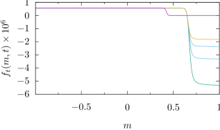
Figure 5: Time derivative of FFE found numerically from Eq. (18) for HTM with the same parameters as in Fig. 2 and for the same five values of evolution time (from bottom to top) as in the text following Eq. (24).

As is seen, the time derivative is constant in the region $m\leq 0$ needed in Eq. (22). Furthermore, it is easy to see that in this range it should be equal to specific rate $\lambda$ from Eq. (24) which means that the distribution of $m$ remains the same throughout the evolution and only the total density of metastable states changes with time according to the exponential law Eq. (22). In fact, because the evolution is very slow it is reasonable to expect that the magnetization distribution should be close to the equilibrium one Eq. (6) as illustrated in Fig. 3. In other words, at negative values of $m$ an accurate solution to EH density should be feasible with the ansatz

$$u(m,t)\simeq\lambda t+v(m,\lambda).$$ (37)

After substitution in Eq. (18) one sees that the time variable disappears from the equation. Also, the two terms in the sum would contain $v_{m}$ at two successive points $m-\epsilon$ and $m+\epsilon$, so if the leftmost $m=-1$ value is known, the rest can be found successively by recursion [26]. But at $m=-1$ only one term remains on the rhs of Eq. (18), so $v(m=-1+\epsilon)$ can be expressed through $\lambda$ and the HTM parameters. Next introducing

$$x_{n+1}=e^{-2[v_{m}(m+\epsilon)-u^{0}_{m}(m+\epsilon)]}-1,$$ (38)

Eq. (18) for $x_{n}$ can be cast in the form of a nonlinear recurrence relation

$$x_{n+1}=a_{n}\frac{x_{n}}{1+x_{n}}+b_{n}$$ (39)

where

$$a_{n}=\frac{1+m}{1-m}e^{2u_{m}^{0}(m+\epsilon)}\frac{1+\exp[-2u_{m}^{0}(m+\epsilon)]}{1+\exp[-2u_{m}^{0}(m-\epsilon)]}$$ (40)

and

$$b_{n}=-\frac{2\lambda}{1-m}\left(1+e^{2u_{m}^{0}(m+\epsilon)}\right).$$ (41)

(Note that in the above equations only subscript $m$ stands for the discrete derivative, all other being just integer numbers.) Thus, from the recurrence relation Eq. (39) all $v(m,\lambda)$ can be found provided a suitable value of $\lambda$ is chosen in Eq. (41). To understand how this can be done, a more careful analysis of Eqs. (39)–(41) is in order.

To this end we first introduce a useful formal rearrangement of the recurrence. As can be seen from Eq. (40), $a_{0}$ is equal to zero so that according to Eq. (39) $x_{1}$ is equal to $b_{0}$. Thus, the recurrence can be initiated by $x_{1}$ which, as can be seen from Eq. (36), has the lowest physically allowed subscript. However, a simpler solution of the linear recurrence in Appendix B is obtained if it is initiated by $x_{0}=0$ and $a_{0}=1$. This is admissible because for $m=-1$ ($n=0$) the first term on the rhs of Eq. (39) vanishes, so with $x_{0}=0$ $a_{0}$ may be ascribed any value.

A trivial solution of the recurrence is obtained with the choice $\lambda=0$. Then from Eqs. (39) and (41) follows that $x_{n}=0$. According to Eq. (38) this means that $v_{m}=u^{0}_{m}$, that is, the equilibrium solution is recovered. This ought to be expected because $\lambda=0$ corresponds to a stationary state. Solutions of Eq. (39) will be convenient to visualize with the use of FFE

$$\tilde{f}(m,\lambda)=v(m,\lambda)-s(m).$$ (42)

Curve 1 in Fig. 6 corresponds to the fully decayed state (barring the remainder $n_{A}\sim 10^{-38}$), i.e., to the equilibrium state $v=u^{0}$.

Figure 6: (Color online) FFE Eq. (42) calculated with the use of Eqs. (39) and (38) for values of $\lambda$ given in Table 1.

Table 1: Values of parameter $\lambda$ for curves shown in Fig. 6 and the fit of data in Fig. 2 to Eq. (22).

Curve	$\lambda\cdot 10^{7}$
1	0.0
2	6.0
3	5.6
4	5.551
5	5.5501
6	5.550092
7	5.5500919602
8	5.5500919601
Fit	5.55009

A less trivial solution can be obtained for small $x_{n}$ satisfying

$$\max|x_{n}|\ll 1$$ (43)

in which case $x_{n}$ in the denominator in Eq. (39) can be neglected and a closed-form solution obtained (see Appendix B)

$$x_{n}=\sum_{l=0}^{n-1}b_{l}\exp\left(\sum_{k=l+1\leq n-1}^{n-1}\ln a_{k}\right).$$ (44)

Using Eq. (41) two immediate conclusions can be made: (i) $x_{n}\propto\lambda$ and (ii) all $x_{n}$ for $n\geq 1$ are negative. Thus, when $\max|x_{n}|\to 1$ or $x_{n}\to-1$ a singularity at a finite $m=-1+2n\epsilon$ will arise in $x_{n}$, hence, also in EH and FFE Eq. (42) which means that the solution is unphysical at this value of $\lambda$.

Thus, the physical values should be sought in the interval $0\leq\lambda\leq\lambda_{max}$ with the upper limit found as the largest $\lambda$ at which the solution does not diverge. This has been done via a trial and error process for the same HTM parameters as in Fig. 2. The results are presented in Fig. 6 and Table 1. The range of calculations has been extended beyond $m=0$ into the region where according to Fig. 5 solution Eq. (37) is still valid. It has been found that $v(m,\lambda)$ is very sensitive to the precise value of $\lambda$ near $\lambda_{max}$. For example, curves 7 and 8 correspond to $\lambda$ values that differ on a unit in the eleventh significant digit. Yet curve 7 shows that the value is still too large (the solution diverges) while curve 8 already goes deep down and if assumed to be correct predicts $n_{A}\sim 10^{-27}$, that is the decay is practically terminated. In fact, the curve is drawn farther than the range of validity of Eq. (39) as can be seen by comparing Figs. 5 and 6. But even at the upper end of the region of validity $m\leq 0.4$ the value of $\tilde{f}$ is such that $n_{A}\sim 10^{-10}$. This, however, is an overestimation because the negative derivative of curve 8 indicates that the true value of $\tilde{f}$ near minimum B should be noticeably smaller. Anyway, we are going to compare the calculated lifetimes with those of Ref. [13] defined as the weighted time averages so the contributions of small $n_{A}(t)$ were insignificant. Thus, in our case a single value of $\lambda_{max}$ should be sufficient to determine the lifetime from Eq. (24). This is consistent with the data shown in Figs. 2 and 5 where $\lambda\approx 5.55009\cdot 0^{-7}$ (see Table 1) was sufficient to describe the decay from $n_{A}\approx 0.9$ to $10^{-12}$. The agreement of $\lambda$ found from the recurrence relation with that determined in a fit to the solution of the exact evolution equation to all six significant digits provided by the fitting software supports the suggestion that the heuristic technique based on recurrence Eq. (39) does make possible an accurate determination of lifetimes of the metastable states in HTM. Similar agreement between the two techniques has been found for several additional sets of HTM parameters.

The values of $\tau$ calculated in this way are shown in Fig. 4 by filled symbols. The excellent agreement with the results of Ref. [13] is illustrated by comparison with the analytic expression Eq. (45) suggested in that paper

$$\tilde{\tau}=\frac{\pi}{\sqrt{|m_{SP}|(h_{SP}-h)}}e^{N\Delta f^{0}}.$$ (45)

where $\Delta f^{0}$ has been defined in Eq. (23). In our calculations the notion of scaling in the vicinity of the spinodal has not been used because in some cases, such as the one depicted in Fig. 1, the simulated systems were quite far from it. Therefore, in order to make comparison with Eq. (41) of Ref. [13] $\Delta f^{0}$ for the barrier height has been used instead of the scaling expression. The comparison with the latter has also been performed with the agreement being only slightly worse than in Fig. 4, arguably, for the above mentioned reason. The upper limit of the data presented in Fig. 4 has been defined by the fact that in order for the calculations were meaningful the second term in the denominator of Eq. (39) $1+x_{n}$ should contribute to the recursion from $n=1$ onward. Therefore, $n_{1}=O(\lambda)$ should exceed the smallest number able to change the result when added to unity. In the double precision arithmetic used in calculations it should be larger than $\sim 2\cdot 10^{-16}$. The use of software with this quantity being much smaller would make possible to predict much larger lifetimes.

In principle, analytical expression of the type of Eq. (45) should be possible to derive from the condition

$$\max|x_{n}|\to 1.$$ (46)

However, this would necessitate knowledge of an analytical expression for $x_{n}$ which is difficult to obtain for $x_{n}\to-1$ where Eq. (39) is strongly nonlinear. However, the leading exponential in $N$ behavior can be estimated in the linear approximation Eq. (44). To this end in the expression Eq. (41) for $b_{n}$ we retain only factor $\lambda$ which needs to be determined and in the summation over $k$ only the first two factors in the expression Eq. (40) will be kept because the last factor does not contribute to the logarithm in the limit $\epsilon\to 0$. With the use of Eq. (12) the first two factors in Eq. (40) can be unified in $\exp[2f^{0}_{m}(m_{k})]$; here and below $m_{n},m_{l}$ and $m_{k}$ are connected to $n,l,k$ via Eq. (36). Next, approximating $2\sum_{l(k)}\approx N\int dm_{l(k)}$ ($dm_{l(k)}\simeq 2/N$) and integrating over $dm_{k}$ one arrives at an estimate

$$\max_{n}|x_{n}| \sim \max_{m_{n}}\lambda e^{Nf^{0}(m_{n})}\int_{-1}^{m_{n}}dm_{l}e^{-Nf^{0}(m_{l})}$$ (47)

$$\sim \lambda e^{N[f^{0}(C)-f^{0}(A)]}\equiv\lambda e^{N\Delta f^{0}}\simeq 1.$$

where the integration over $m_{l}$ for large $N$ has been estimated by Laplace’s method, and within the range of validity of Eq. (39) the maximum is attained at $m_{n}=m_{C}$. The estimate Eq. (23) now follows from Eq. (24).

To conclude this section, a few words about the decay of unstable states when $h>h_{SP}$ (in the geometry of Fig. 1) which was also studied in Ref. [13]. This case has not been detailed in the present paper because of its complexity. While the decay of metastable states has a clear underlying physics of the escape over the energy barrier, the unstable case is governed by at least two competing mechanisms. First, because there is no local minimum in $f^{0}$ at $m_{A}$, at large $h\gg h_{SP}$ the minimum in Eq. (19) will be moving toward $m_{B}$ according to MF Eq. (34) in which case the time dependence of $n_{A}$ will be close to the step function $\theta(-m_{0}(t))$. However, near the spinodal when $h$ approaches $h_{SP}$ from above the MF evolution slows down [13] and the diffusion mechanism starts to dominate. The exponential behavior similar to Eq. (22) has been observed for $h\to h_{SP}^{+}$ but in the absence of the double-well structure of $f^{0}$ its origin is obscure. The second minimum at $m_{B}$ has been formed which presupposes the existence of the barrier in FFE $f$ but whether this kinetically induced shape may play the same role as the double-well structure of equilibrium $f^{0}$ for $h>h_{SP}$ is not clear. Besides, because the initial NPD is to a large extent arbitrary the FFE shape will strongly depend on it. Therefore, additional insights are needed to explain the complexities of the decay of unstable states.

VII Conclusion

In this paper a nonlinear master equation (NLME) describing time evolution of the effective Hamiltonian (EH) density has been suggested to overcome the numerical difficulties caused by the presence in the conventional linear ME [7] of quantities exponentially depending on the system size $N$. In contrast, NLME scales at most as $O(N)$. In the Ising models with short range interactions NLME is strongly nonlinear hence, difficult to solve. However, this should not be surprising because NLME is supposed to describe all possible non-equilibrium phenomena that may arise during the evolution starting from any of the uncountable number of possible initial conditions.

To illustrate some salient features of NLME in a simple framework, the problem of decay of metastable states in the kinetic Husimi-Temperley model (HTM) has been considered. The problem was previously studied in the framework of linear equations in Refs. [10, 11, 13] which data have been used for comparison purposes. An excellent agreement has been found between numerical NLME results and the asymptotic analytic expression for the lifetime of the metastable state of Ref. [13]. With the use of NLME it has been possible to cover much broader range of HTM parameters and to achieve much better accuracy.

The exponential dependence of lifetime on the system size ensures that in macroscopic systems the lifetime will reach values so large that from physical standpoint the metastable states will behave as effectively stable ones. Because of this, for large $N$ it is reasonable to take the thermodynamic limit $N\to\infty$. It has been shown that in this case NLME simplifies to a nonlinear first-order differential equation possessing, in particular, two locally stable solutions which can be combined to construct stationary EHs different from the equilibrium one. To solve the differential equation a system of characteristic equations has been derived which, in particular, reduces to the conventional MF equation [15] for magnetizations corresponding to the fluctuating free energy extrema.

It seems counterintuitive to switch from a linear equation to a nonlinear one. However, this seems to be a common way of dealing with many-body problems. In the case of ME this was discussed in Ref. [7] (see Remark in Ch. V.8) where it was argued that a linear/nonlinear dichotomy is purely mathematical and does not reflect the underlying physics. For example, the linear Liouville equation is equivalent to Newton’s equations which in the case of interacting particles are nonlinear, yet it is the latter that are used in practical calculations.

A promising example of NLME use was discussed in Ref. [4]. In a simple pair approximation to EH which was also successfully used in Ref. [27] it was found that NLME leads to a qualitatively more sound description of the spinodal decomposition than the MF approximation to ME used, e.g., in Ref. [3]. Namely, NLME predicted a power-law growth of the volumes of separating phases while the MF approximation produces an exponential behavior. The latter is incompatible with the relaxational nature of the stochastic dynamics where the growth exponents cannot be positive [7]. Besides, the characteristic length scale in the MF solution remains constant throughout the growth while NLME predicts a coarse-graining behavior in accordance with experiment.

Yet another example is the BBGKY hierarchy of an infinite number of linear equations which in practical calculations is usually approximated by a finite number of nonlinear equations, such as the Boltzmann transport equation.

Thus, it is quite plausible that NLME is a proper way of dealing with stochastic kinetics of Ising-type models.

Appendix A The Hamilton-Jacobi formalism

Because Eq. (29) contains only derivatives of $u$ but not the function itself, according to Ref. [24] it can be cast in the form of the Hamilton–Jacobi equation [28]

$$u_{t}+\mathbf{H}(m,q,t)=0,$$ (48)

where

$$q=u_{m}(m,t)$$ (49)

and

$$\mathbf{H}=-\cosh^{2}q\,(m+\tanh q)[\tanh{u}^{0}_{m}(m,t)-\tanh q]$$ (50)

is the rhs of Eq. (29) with minus sign. In the Hamiltonian formalism the total time derivative of any function $g(m,q,t)$ of the “coordinate” $m$ and “momentum” $q$ can be calculated as

$$\dot{g}\equiv\frac{dg}{dt}=\frac{\partial g}{\partial t}+\{g,\mathbf{H}\},$$ (51)

where the Poisson bracket is defined as $\{a,b\}=a_{m}b_{q}-a_{q}b_{m}$. Now the canonical Hamiltonian equations are easily found as

$$\dot{m} = \mathbf{H}_{q}$$ (52)

$$\dot{q} = -\mathbf{H}_{m}.$$ (53)

Further assuming that at some $t=t_{0}$ an initial Hamiltonian density $u(m,t_{0})$ is known, by choosing any admissible value $m_{0}$ and setting $q(t_{0})$ equal to $u_{m}(m_{0},t_{0})$ one can find $m(t)$ and $q(t)$ from the solution of the initial value problem for Eqs. (52) and (53). Next integrating equation

$$\dot{u}=q\mathbf{H}_{q}-\mathbf{H}$$ (54)

obtained from Eqs. (51), (52), (49), and (48) one arrives at a solution for $u(m,t)$ in parametric form where at each $t$ the values of $u$ at different $m$ are found from the solution of the above initial-value problem for all possible $m_{0}=m(t_{0})$. Such a solution is a particular case of the general method of characteristics [23].

A rigorous derivation of the Hamiltonian-Jacobi formalism in the general case of many variables can be found in Ref. [24] but for our Eq. (48) the following heuristic arguments should suffice. First we observe that the partial derivative $u_{m}$ in Eq. (29) couples the values of function $u(m,t)$ at neighbor points $m\pm\epsilon$ so by using, e.g., the method of lines one should solve a system of $N\to\infty$ coupled ordinary evolution equations. In the method of characteristics one tries to reduce the problem to only a few such equations. To this end one may observe that by taking the total time derivative of Eq. (49) in the conventional way one gets

$$\dot{q}=u_{mt}+u_{mm}\dot{m}=-\mathbf{H}_{m}-\mathbf{H}_{q}u_{mm}+u_{mm}\dot{m}$$ (55)

where the second equality has been obtained by differentiating Eq. (48) with respect to $m$ by considering $q$ in $\mathbf{H}$ as just another notation for $u_{m}$. Now if we demand that Eq. (52) was satisfied, than Eq. (53) would follow from Eq. (55). Eq. (54) also is easily obtained by differentiating $u(m,t)$, using Eq. (48 and applying the chain rule. Next assuming $m=m(t)$ on the characteristic line, substituting it in Eqs. (52), (53), and (54) one arrives at a system of three evolution equations for three unknown functions. It is to be noted that Eqs. (52) and (53) are sufficient to derive Eq. (51) which shows the consistency of our assumptions.

Appendix B Linear recurrence [26]

Let us consider a linear recurrence relation

$$x_{n+1}=a_{n}x_{n}+b_{n}$$ (56)

initiated by $x_{0}$; $a_{n}$ and $b_{n}$, $n=0,N$ are presumed to be known. Now by introducing

$$X_{n}=\frac{x_{n}}{\prod_{k=0}^{n-1}a_{k}}$$ (57)

and dividing both sides of Eq. (56) by $\prod_{k=0}^{n}a_{k}$ one arrives at a linear difference equation

$$X_{n+1}-X_{n}=b_{n}/\prod_{k=0}^{n}a_{k}$$ (58)

which can be solved as

$$X_{n}=X_{0}+\sum_{l=0}^{n-1}\frac{b_{l}}{\prod_{k=0}^{l}a_{k}}.$$ (59)

In the main text it was assumed that $x_{0}=0$ which in combination with Eq. (57) gives $X_{0}=0$ and

$$x_{n}=\sum_{l=0}^{n-1}b_{l}\prod_{k=l+1\leq n-1}^{n-1}a_{k}=\sum_{l=0}^{n-1}b_{l}\exp\left(\sum_{k=l+1\leq n-1}^{n-1}\ln a_{k}\right).$$ (60)

References

- Huang [1987] K. Huang, Statistical Mechanics, 2nd ed. (John Wiley & Sons, 1987).
- Ducastelle [1991] F. Ducastelle, Order and Phase Stability in Alloys (North-Holland, Amsterdam, 1991).
- Gouyet et al. [2003] J.-F. Gouyet, M. Plapp, W. Dieterich, and P. Maass, Description of far-from-equilibrium processes by mean-field lattice gas models, Adv. Phys. 52, 523 (2003).
- Tokar [1996] V. I. Tokar, Hamiltonian approach to the kinetic Ising models, Phys. Rev. E 53, 1411 (1996).
- Vaks [1996] V. G. Vaks, Master equation approach to the configurational kinetics of nonequilibrium alloys: exact relations, -theorem, and cluster approximations., JETP Lett. 63, 471 (1996).
- Nastar et al. [2000] M. Nastar, V. Dobretsov, and G. Martin, Self-consistent formulation of configurational kinetics close to equilibrium: The phenomenological coefficients for diffusion in crystalline solids, Phil. Mag. A 80, 155 (2000).
- Van Kampen [1992] N. Van Kampen, Stochastic Processes in Physics and Chemistry (Elsevier Science, 1992).
- Glauber [1963] R. J. Glauber, Time‐dependent statistics of the Ising model, J. Math. Phys. 4, 294 (1963).
- Kawasaki [1966] K. Kawasaki, Diffusion constants near the critical point for time-dependent Ising models. I, Phys. Rev. 145, 224 (1966).
- Tomita et al. [1976] H. Tomita, A. Itō, and H. Kidachi, Eigenvalue problem of metastability in macrosystem, Prog. Theo. Phys. 56, 786 (1976).
- Matkowsky et al. [1984] B. J. Matkowsky, Z. Schuss, C. Knessl, C. Tier, and M. Mangel, Asymptotic solution of the Kramers-Moyal equation and first-passage times for Markov jump processes, Phys. Rev. A 29, 3359 (1984).
- Chakrabarti and Acharyya [1999] B. K. Chakrabarti and M. Acharyya, Dynamic transitions and hysteresis, Rev. Mod. Phys. 71, 847 (1999).
- Mori et al. [2010] T. Mori, S. Miyashita, and P. A. Rikvold, Asymptotic forms and scaling properties of the relaxation time near threshold points in spinodal-type dynamical phase transitions, Phys. Rev. E 81, 011135 (2010).
- Carinci [2013] G. Carinci, Random hysteresis loops, Ann. Inst. H. Poincaré Probab. Statist. 49, 307 (2013).
- Suzuki and Kubo [1968] M. Suzuki and R. Kubo, Dynamics of the Ising model near the critical point. I, J. Phys. Soc. Jpn. 24, 51 (1968).
- Tomé and de Oliveira [1990] T. Tomé and M. J. de Oliveira, Dynamic phase transition in the kinetic Ising model under a time-dependent oscillating field, Phys. Rev. A 41, 4251 (1990).
- Sanchez et al. [1984] J. Sanchez, F. Ducastelle, and D. Gratias, Generalized cluster description of multicomponent systems, Physica A 128, 334 (1984).
- Asta et al. [1991] M. Asta, C. Wolverton, D. de Fontaine, and H. Dreyssé, Effective cluster interactions from cluster-variation formalism. I, Phys. Rev. B 44, 4907 (1991).
- Wolverton and Zunger [1997] C. Wolverton and A. Zunger, Ni-Au: A testing ground for theories of phase stability, Comput. Mater. Sci. 8, 107 (1997), proceedings of the joint NSF/CNRS Workshop on Alloy Theory.
- Kramers [1940] H. A. Kramers, Brownian motion in a field of force and the diffusion model of chemical reactions, Physica 7, 284 (1940).
- Hänggi et al. [1990] P. Hänggi, P. Talkner, and M. Borkovec, Reaction-rate theory: fifty years after Kramers, Rev. Mod. Phys. 62, 251 (1990).
- Zhu et al. [2004] H. Zhu, S. Dong, and J.-M. Liu, Hysteresis loop area of the Ising model, Phys. Rev. B 70, 132403 (2004).
- Whitham [2011] G. Whitham, Linear and Nonlinear Waves, Pure and Applied Mathematics: A Wiley Series of Texts, Monographs and Tracts (Wiley, 2011).
- Kamke [1959] E. Kamke, Differentialgleichungen Lösungsmethoden und Lösungen. Band II: Partielle Differentialgleichungen erster Ordnung für eine gesuchte Funktion (Akademische Verl. Ges., Leipzig, 1959).
- Cugliandolo [2015] L. F. Cugliandolo, Coarsening phenomena, C. R. Phys. 16, 257 (2015).
- Wikimedia Foundation [2023a] Wikimedia Foundation, Recurrence relation, https://en.wikipedia.org/wiki/Recurrence_relation (2023a), Last accessed 08/05/2023.
- Nastar [2005] M. Nastar, A mean field theory for diffusion in a dilute multi-component alloy: a new model for the effect of solutes on self-diffusion, Phil. Mag. 85, 3767 (2005).
- Wikimedia Foundation [2023b] Wikimedia Foundation, Hamilton–jacobi equation, https://en.wikipedia.org/wiki/Hamilton-Jacobi_equation (2023b), Last accessed 05/21/2023.