Inverse Dynamics Trajectory Optimization for Contact-Implicit Model Predictive Control

Abstract

Robots must make and break contact with the environment to perform useful tasks, but planning and control through contact remains a formidable challenge. In this work, we achieve real-time contact-implicit model predictive control with a surprisingly simple method: inverse dynamics trajectory optimization. While trajectory optimization with inverse dynamics is not new, we introduce a series of incremental innovations that collectively enable fast model predictive control on a variety of challenging manipulation and locomotion tasks. We implement these innovations in an open-source solver and present simulation examples to support the effectiveness of the proposed approach. Additionally, we demonstrate contact-implicit model predictive control on hardware at over 100 Hz for a 20-degree-of-freedom bi-manual manipulation task. Video and code are available at https://idto.github.io.

I Introduction

Contact is critical for legged locomotion and dexterous manipulation, but most optimization-based controllers assume a fixed contact sequence [1]. Contact-Implicit Trajectory Optimization (CITO) aims to relax this assumption by solving jointly for the contact sequence and a continuous motion. A sufficiently performant CITO solver would enable Contact-Implicit Model Predictive Control (CI-MPC), allowing robots to determine contact modes on the fly and perform more complex tasks.

Despite growing interest in CITO, fast and reliable CI-MPC remains elusive. Most existing methods take either a direct approach [2, 3, 4, 5, 6, 7, 8, 9], in which decision variables represent state and control at each time step, or a shooting approach [10, 11, 12, 13, 14, 15, 16], where control inputs are the only decision variables. Both work well for smooth dynamical systems, but struggle to handle contact. The large number of additional constraints used to model contact, rank deficiency, and ill conditioning have a large impact on numerics, which degrades robustness, convergence, and ultimately, performance. Other issues include the difficulty of initializing and/or warm-starting variables, locally optimal solutions that do not obey physics, and high sensitivity to problem parameters. Much active research focuses on solving these problems.

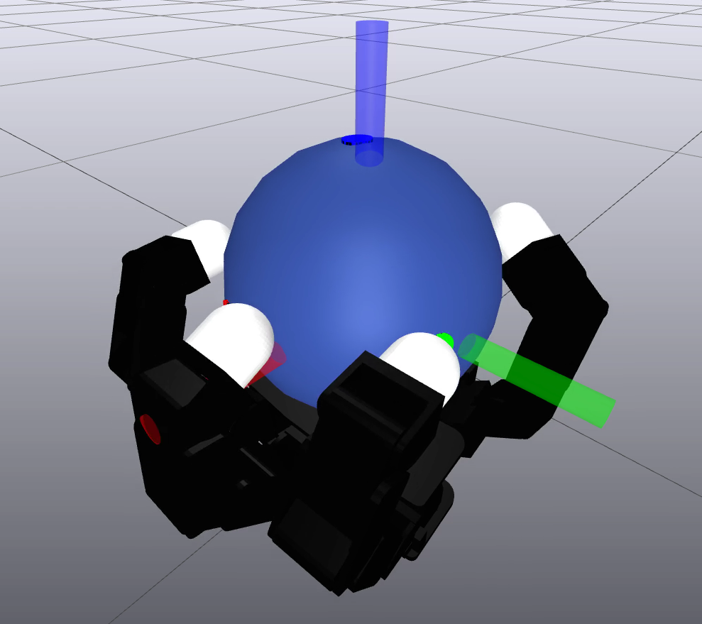
(a) Dexterous Hand: 10 Hz

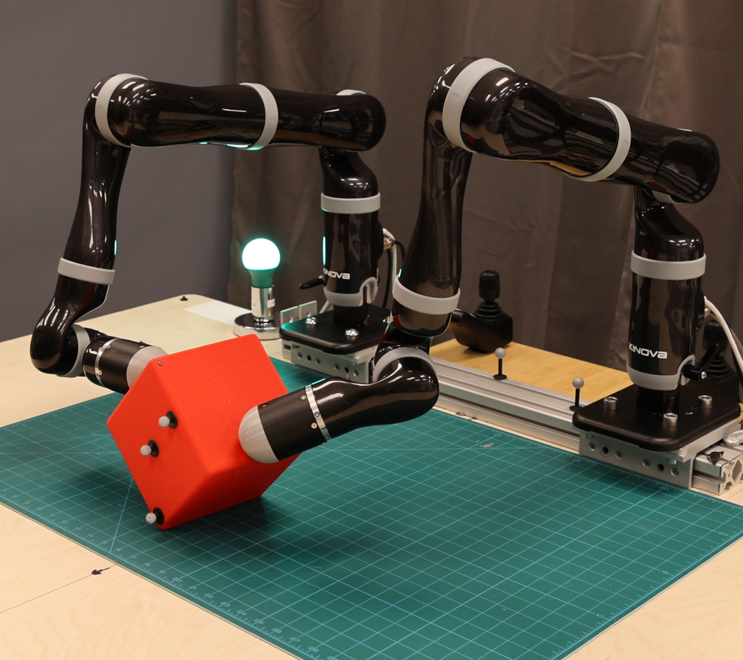
(b) Bi-manual Manip.: 100 Hz

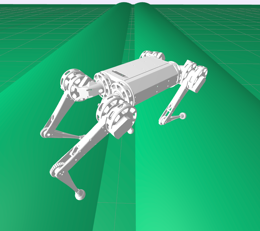
(c) Quadruped: 60 Hz

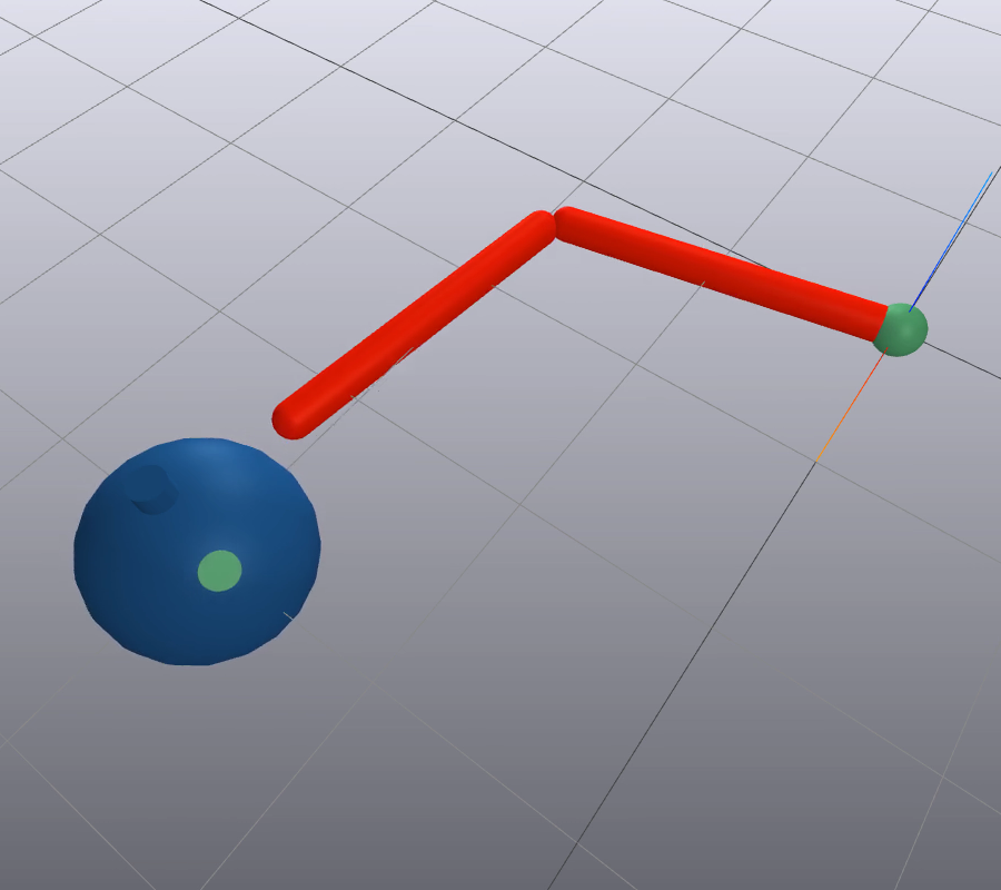
(d) Spinner: 200 Hz

Figure 1: IDTO enables real-time CI-MPC on a variety of challenging manipulation and locomotion tasks. Contact sequences, locations, and timings are all determined automatically by the solver over a horizon of 1-2 seconds.

Here, we adopt a less popular approach, Inverse Dynamics Trajectory Optimization (IDTO) [17, 18], and show that it enables fast and effective CI-MPC. Instead of constraints, IDTO uses compliance and regularized friction to formulate an optimization problem where generalized positions are the only decision variables. We cast this optimization as a least squares problem, for which we develop a custom trust-region solver. This solver leverages a series of small innovations—a smooth and compliant contact model, scaling, sparse Hessian factorization, and an equality-constrained dogleg method—to achieve state-of-the-art performance. Our IDTO solver enables real-time CI-MPC on various challenging tasks, including on hardware, as illustrated in Fig. 1.

II Related Work

This section reviews related literature, categorizing methods based on offline CITO versus online CI-MPC.

II-A Offline Contact-Implicit Trajectory Optimization

CITO aims to optimize the robot’s trajectory, contact forces, and actuation. Different formulations exist.

Direct methods introduce decision variables for both state and control, and enforce the dynamics with constraints [2, 3, 4, 5, 6, 7]. This results in a large but sparse nonlinear program. Direct methods support arbitrary constraints and infeasible initializations. However, the large number of nonlinear constraints used to model dynamics and contact lead to a large optimization problem, which is difficult to solve efficiently. Moreover, these formulations can fall into local minima that might not obey the laws of physics [19].

Shooting methods like Differential Dynamic Programming (DDP) [20] and iterative LQR (iLQR) [21] introduce decision variables only for the control, and are increasingly popular for CITO [10, 11, 12, 13, 14, 15]. These methods enforce dynamics with forward rollouts, so each iteration is dynamically feasible. On the other hand, designing an informative initial guess can be challenging, and it is difficult to include constraints. Additionally, each rollout simulates contact dynamics to high precision, which usually requires solving an optimization sub-problem for each time step [22]. Combining the flexibility of direct methods with the defect-free integration of shooting is an area of active research [23, 24, 25, 26].

II-B Contact-Implicit Model Predictive Control

The earliest simulated CI-MPC [10] ran in real time for low-dimensional problems, but could not maintain real-time performance for larger systems. The first hardware implementation [27] emerged several years later, though this method required extensive parameter tuning.

Recent years have seen numerous exciting advancements in CI-MPC. MuJoCo MPC [28] enables real-time CI-MPC for a number of larger systems (quadrupeds, humanoids, etc.) using various algorithms, though these methods have not yet been validated on hardware. [9] achieves quadruped CI-MPC on hardware with a bi-level scheme, performing more expensive computations offline about a reference trajectory and solving smaller problems online with a sparse interior-point solver.

A hybrid-systems iLQR method [16], with sophisticated mechanisms for handling unexpected contact mode transitions, enables real-time CI-MPC on a quadruped. Another hybrid MPC approach based on the Alternating Direction Method of Multipliers (ADMM) [8] breaks the dependence of the contact-scheduling problem between time steps, allowing parallelization. The method in [8] is tested on hardware.

II-C Inverse Dynamics Trajectory Optimization

While most existing work treats inputs as the decision variables (shooting methods) or states and inputs as the decision variables (most direct methods), IDTO uses only generalized positions [17].

This offers several advantages. Inverse dynamics are faster to compute than the forward dynamics needed in shooting methods [29]. Unlike typical direct methods, IDTO does not require complex dynamics constraints, and uses compliant contact to eliminate the need for contact constraints. Early CITO work used IDTO and simplified physics to synthesize contact-rich behaviors for animated characters [30, 31]. [17] proposed a physically consistent version, and Emo Todorov described a more mature implementation in Optico, an unreleased software package, in several talks [18, 32]. Our work is heavily inspired by Optico, though we believe our solver differs in a number of important respects. We use trust region rather than linesearch, for example, and handle underactuation differently.

III Contribution

In this paper, we show that IDTO enables real-time CI-MPC for complex systems like those shown in Fig. 1. We detail design choices for the formulation as a least-squares problem and a custom solver for that problem.

Our implementation is available at https://idto.github.io. We describe implementation details, characterize numerics and convergence, and evaluate performance. We validate our solver in simulation for a variety of dexterous manipulation and legged locomotion tasks, as well as on hardware for bi-manual manipulation.

Our approach is not perfect, nor is it the ultimate CI-MPC solution. We strove to make simple design choices whenever possible, with the hope that this will illuminate key challenges and enable better solutions in the future. To this end, we provide an extensive discussion of the limitations of our approach in Section VIII.

IV Nonlinear Least-Squares Formulation

We closely follow the notation of our previous work on contact modeling for simulation [33, 22]. We use $\bm{x}=[\bm{q}~{}\bm{v}]$ to describe the state of a multibody system, consisting of generalized positions $\bm{q}\in\mathbb{R}^{n_{q}}$ and generalized velocities $\bm{v}\in\mathbb{R}^{n_{v}}$. Time derivatives of the positions relate to velocities by the kinematic map $\bm{N}(\bm{q})\in\mathbb{R}^{n_{q}\times n_{v}}$,

$$\dot{\bm{q}}=\bm{N}(\bm{q})\bm{v}.$$ (1)

$\bm{N}(\bm{q})$ is the identity matrix in most cases, though not for quaternion Degrees of Freedom (DoFs).

We consider CITO problems of the form

$$\min_{\bm{x},\bm{u}}~{} \int_{t=0}^{T}\ell\big{(}\bm{x}(t),\bm{u}(t),t\big{)}dt+\ell_{f}\big{(}\bm{x}(T)\big{)},$$ (2a)

$$\mathrm{s.t.~{}} \bm{M}(\bm{q})\dot{\bm{v}}+\bm{k}(\bm{q},\bm{v})=\bm{B}\bm{u}+\bm{J}^{T}\bm{f},$$ (2b)

$$\bm{x}(0)=\bm{x}_{0}.$$ (2c)

The cost (2a) encodes the task and penalizes actuation, where $\ell$ and $\ell_{f}$ are running and terminal costs respectively. The problem is constrained to satisfy the equations of motion (2b), where $\bm{M}$ is the mass matrix, $\bm{k}$ collects gyroscopic terms, gravitational forces and joint damping, and $\bm{B}$ maps actuation inputs $\bm{u}\in\mathbb{R}^{n_{u}}$ to actuated DoFs. The dynamics (2b) include both the robot and objects in the environment. For a set of $n_{c}$ contact constraints, contact forces $\bm{f}\in\mathbb{R}^{3n_{c}}$ are applied through the contact Jacobian $\bm{J}\in\mathbb{R}^{3n_{c}\times n_{v}}$. Finally, (2c) provides the initial condition at time $t=0$.

IV-A Contact Kinematics

Given a configuration $\bm{q}$, our contact engine reports a set of $n_{c}$ contact pairs. We characterize the $i\text{-th}$ pair by its location, signed distance $\phi_{i}(\bm{q})\in\mathbb{R}$ and contact normal $\widehat{\bm{n}}_{i}$, see [22] for details. The relative velocity at the contact point is denoted $\bm{v}_{c,i}$, and relates to generalized velocities via the $i\text{-th}$ row of the contact Jacobian. We split the contact velocity into its normal component $v_{n,i}=\widehat{\bm{n}}_{i}\cdot\bm{v}_{c,i}$ and tangential component $\bm{v}_{t,i}=\bm{v}_{c,i}-v_{n,i}\widehat{\bm{n}}_{i}$, so that $\bm{v}_{c,i}=[v_{n,i}~{}\bm{v}_{t,i}]$. For brevity, we omit the contact subscript $i$ from now on.

IV-B Contact Modeling

Many CITO formulations augment (2) with additional decision variables and constraints to model contact forces that satisfy Coulomb friction and the principle of maximum dissipation. Building on our experience in contact modeling for simulation [33, 22], we adopt a simpler approach based on compliant contact with regularized friction. With this approach, contact forces are a function of the state. Unlike the accurate and often stiff models used for simulation, however, here we focus on algebraic forms that are continuously differentiable and thus more suitable for trajectory optimization.

As with the contact velocity, we split the contact force at each contact point into its normal $f_{n}$ and tangential $\bm{f}_{t}$ components such that $\bm{f}_{c}=[f_{n}~{}\bm{f}_{t}]$.

We model the normal force as

$$f_{n}=c(\phi)d(v_{n}),$$ (3)

where

$$c(\phi)=\sigma k\log\left(1+\exp(-\phi/\sigma)\right)$$ (4)

provides a smooth model of compliance that approximates a linear spring of stiffness $k$ in the limit to zero smoothing parameter $\sigma$. While $\sigma$ can be thought of as the scale parameter of a logistic distribution over signed distances $\phi$ [34], here we use it to trade off smoothness and force at a distance.

We model dissipation as

$$d(v_{n})=\begin{cases}1-\frac{v_{n}}{v_{d}}&\text{if }\frac{v_{n}}{v_{d}}<0,\\ (\frac{v_{n}}{v_{d}}-2)^{2}/4&\text{if }0\leq\frac{v_{n}}{v_{d}}<2,\\ 0&\text{if }2\leq\frac{v_{n}}{v_{d}},\end{cases}$$ (5)

a smoothed Hunt and Crossley model [35] with dissipation velocity $v_{d}=1/d_{HC}$ defined as the reciprocal of the Hunt and Crossley dissipation parameter $d_{HC}$.

We model the tangential component $\bm{f}_{t}$ with a regularized model of Coulomb friction

$$\bm{f}_{t}=-\mu\frac{\bm{v}_{t}}{\sqrt{v_{s}^{2}+\|\bm{v}_{t}\|^{2}}}\,f_{n},$$ (6)

where $\mu$ is the friction coefficient and $v_{s}$ is the stiction tolerance. This model satisfies both the model of Coulomb friction ($\|\bm{f}_{t}\|\leq\mu f_{n}$) and the principle of maximum dissipation (friction opposes velocity) at the expense of drift during stiction at speeds lower than $v_{s}$.

IV-C Inverse Dynamics Trajectory Optimization

In this section, we approximate (2) as a nonlinear least squares problem. The key idea is to use generalized positions $\bm{q}$ as the only decision variables and enforce dynamic feasibility with inverse dynamics.

We will focus on quadratic cost terms of the form

$$\ell(\bm{x},\bm{u},t)=\frac{1}{2}\|\bm{x}(t)-\bar{\bm{x}}(t)\|^{2}_{\bm{Q}}+\frac{1}{2}\|\bm{u}(t)\|^{2}_{\bm{R}},$$

$$\ell_{f}(\bm{x})=\frac{1}{2}\|\bm{x}(T)-\bar{\bm{x}}(T)\|^{2}_{\bm{Q}_{f}},$$ (7)

where $\bm{Q}$, $\bm{R}$, and $\bm{Q}_{f}$ are diagonal scaling matrices and $\bar{\bm{x}}(\cdot)$ is a nominal trajectory. $\bar{\bm{x}}(\cdot)$ provides a rough description of the desired behavior and is not necessarily dynamically feasible.

We discretize the time horizon into $N$ steps of size $\delta t$ and approximate (2a) using a first-order quadrature rule

$$L(\bm{x},\bm{u})=\sum_{k=0}^{N}\ell_{k}(\bm{x}_{k},\bm{u}_{k}),$$ (8)

where for convenience we define the total cost $L(\bm{x},\bm{u})$, $\ell_{k}=\delta t\ell(\bm{x}_{k},\bm{u}_{k})$, and $\ell_{N}=\ell_{f}(\bm{x}_{N})$.

We then proceed to write (8) in terms of generalized positions $\bm{q}$. Velocities $\bm{v}$ are a function of $\bm{q}$ as follows,

$$\bm{v}_{k}(\bm{q})=\bm{N}^{+}(\bm{q}_{k})\frac{\bm{q}_{k}-\bm{q}_{k-1}}{\delta t}\quad\forall k=1\dots N,$$ (9)

where $\bm{N}^{+}(\bm{q}_{k})$ is the left pseudoinverse of the kinematic mapping matrix (1). $\bm{v}_{0}=\bm{v}(0)$ is given by (2c).

Similarly, we approximate accelerations $\bm{a}$ as

$$\bm{a}_{k}(\bm{q})=\frac{\bm{v}_{k+1}(\bm{q})-\bm{v}_{k}(\bm{q})}{\delta t}\quad\forall k=0\dots N-1.$$ (10)

Note that we use $k+1$ and $k$ for accelerations, while we use $k$ and $k-1$ for velocities. This leads to $\bm{a}_{k}$ that depend symmetrically on $\bm{q}_{k-1}$, $\bm{q}_{k}$, and $\bm{q}_{k+1}$.

We write contact forces $\bm{f}$ as a function of $\bm{q}$ using the compliant contact model outlined in Section IV-B,

$$\bm{f}_{k}(\bm{q})=\bm{f}(\bm{q}_{k+1},\bm{v}_{k+1}(\bm{q}))\quad\forall k=0\dots N-1.$$ (11)

Finally, we use inverse dynamics to define the generalized forces $\bm{\tau}_{k}$ needed to advance the state from time step $k$ to time step $k+1$,

$$\bm{\tau}_{k}(\bm{q})=\bm{M}(\bm{q}_{k+1})\bm{a}_{k}+\bm{k}(\bm{q}_{k+1},\bm{v}_{k+1})\\ -\bm{J}^{T}(\bm{q}_{k+1})\bm{f}_{k}(\bm{q}_{k+1},\bm{v}_{k+1}).$$ (12)

When compared to a time-stepping scheme for simulation [22], all terms are evaluated implicitly. We make this choice based on the intuition that implicit time-stepping schemes are stable even for stiff systems of equations. Whether this intuition is accurate or useful in the IDTO setting is an area for future study.

For fully actuated systems, generalized forces equal control torques, $\bm{\tau}_{k}=\bm{u}_{k}$. In the more typical underactuated case, we have $\bm{\tau}_{k}=\bm{B}\bm{u}_{k}$, and some entries of $\bm{\tau}_{k}$ must be zero.

Substituting both $\bm{\tau}_{k}$ and $\bm{x}_{k}=[\bm{q}_{k}~{}\bm{v}_{k}]$ as functions of $\bm{q}$ in (8), we can approximate (2) as,

$$\min_{\bm{q}}~{} L(\bm{q}),$$ (13a)

$$\mathrm{s.t.~{}} \bm{h}(\bm{q})=0,$$ (13b)

where $\bm{h}(\bm{q})$ collects unactuated rows of $\bm{\tau}_{k}(\bm{q})$.

Remark 1.

This is a nonlinear least squares problem with equality constraints. To see this, define the residual

$$\bm{r}(\bm{q})=\begin{bmatrix}\bm{\tilde{Q}}^{1/2}(\bm{x}(\bm{q})-\bar{\bm{x}})\\ \bm{\tilde{R}}^{1/2}\bm{\tau}(\bm{q})\end{bmatrix}$$ (14)

where $\bm{\tilde{Q}}$ and $\bm{\tilde{\bm{R}}}$ denote the diagonal matrices that result from stacking $\bm{Q}$ and $\bm{R}$. We can then write the cost in standard least squares form: $L(\bm{q})=1/2\|\bm{r}(\bm{q})\|^{2}$.

V Gauss-Newton Trust-Region Solver

In this section, we develop a solver tailored to (13).

V-A The Unconstrained Problem

We start by considering the unconstrained problem, for which we choose a trust-region method. At each iteration $i$, this method finds an update $\bm{q}^{i+1}=\bm{q}^{i}+\bm{p}$ by solving a quadratic approximation of (13) around $\bm{q}^{i}$,

$$\min_{\bm{p}}~{} L^{i}+\bm{g}^{T}\bm{p}+\frac{1}{2}\bm{p}^{T}\bm{H}\,\bm{p}$$ (15a)

$$\mathrm{s.t.}~{} \|\bm{D}^{-1}\bm{p}\|\leq\Delta,$$ (15b)

where $L^{i}=L(\bm{q}^{i})$ and $\bm{g}=\nabla L(\bm{q}^{i})$ are the cost and its gradient. Matrix $\bm{H}$ is a Gauss-Newton approximation of the Hessian, see Section V-C for details. At each iteration, the trust-region constraint (15b) limits the size of the step $\bm{p}$. We use a diagonal matrix $\bm{D}$ to scale the problem and improve numerical conditioning. Stiff contact dynamics result in a cost landscape with narrow valleys and steep walls. This makes scaling critical for good performance, as illustrated in Fig. 2. We tried various strategies outlined in [36], and found that $\mathrm{diag}(\bm{D})=\mathrm{diag}(\bm{H})^{-1/4}$ gave the best results.

Since solving (15) exactly would be computationally expensive, we use the dogleg method [37, §4.1] to find an approximate solution. This requires a single update and factorization of $\bm{H}$ per iteration. After each iteration, we update the trust-region radius $\Delta$ according to the strategy outlined in [37, Algorithm 4.1].

Figure 2: Convergence plot for the Allegro hand example with and without scaling.

Remark 2.

We chose trust region over linesearch for several reasons. One is speed: each evaluation of the cost $L(\bm{q})$ is expensive, and trust region requires us to compute $L(\bm{q})$ only once per iteration. Trust region is also appealing because $\bm{H}$ is poorly conditioned. In some extreme instances, this can lead to Gauss-Newton search directions ($\bm{p}=-\bm{H}^{-1}\bm{g}$) that are not actually descent directions. Trust-region methods turn toward gradient descent as the trust radius is reduced, which helps avoid this issue.

V-B Handling Equality Constraints

For systems of practical interest with unactuated DoFs, enforcing (13b) is critical for dynamic feasibility. We consider two methods to handle this constraint.

V-B1 Quadratic Penalty

This method adds a penalty of the form $\frac{w}{2}\|\bm{h}(\bm{q})\|^{2}$ to the cost $L(\bm{q})$, where $w$ is a large scalar weight. In practice we implement this by placing $w$ at elements of $\bm{R}$ that correspond to unactuated DoFs.

V-B2 Lagrange Multipliers

The penalty method is simple to implement, and worked well in many cases. However, it cannot entirely drive unactuated torques to zero without high penalties that worsen numerics.

As an alternative, we developed a constrained dogleg method based on Lagrange multipliers. We start with a constrained Newton step

$$\begin{bmatrix}\bm{H}&\bm{A}^{T}\\ \bm{A}&\bm{0}\end{bmatrix}\begin{bmatrix}\bm{p}\\ \bm{\lambda}\end{bmatrix}=\begin{bmatrix}-\bm{g}\\ -\bm{h}\end{bmatrix},$$ (16)

where $\bm{A}$ is the Jacobian of $\bm{h}$ and $\bm{\lambda}$ is a vector of Lagrange multipliers. Since our Hessian approximation is invertible, we can eliminate $\bm{p}$ from (16) and solve for

$$\bm{\lambda}=(\bm{A}\,\bm{H}^{-1}\bm{A}^{T})^{-1}(\bm{h}-\bm{A}\bm{H}^{-1}\bm{g}).$$ (17)

We then solve (16) for the Newton step

$$\bm{p}=-\bm{H}^{-1}(\bm{A}^{T}\bm{\lambda}+\bm{g}).$$ (18)

We can view this step as the unconstrained minimizer of a quadratic model of the merit function

$$L(\bm{q})+\bm{h}(\bm{q})^{T}\bm{\lambda}.$$ (19)

This observation motivates a trust-region variant, where we minimize a quadratic model of (19) subject to bounds on the step size. More formally, the new trust-region subproblem is given by

$$\min_{\bm{p}}~{} L+(\bm{g}+\bm{A}^{T}\bm{\lambda})^{T}\bm{p}+\frac{1}{2}\bm{p}^{T}\bm{H}\bm{p}$$ (20a)

$$\mathrm{s.t.}~{} \|\bm{D}^{-1}\bm{p}\|\leq\Delta,$$ (20b)

which we can solve with the dogleg method. This approach is similar to Fletcher’s smooth exact penalty method [37], albeit with a slightly different approximation of the Lagrange multipliers $\bm{\lambda}$.

Computing $\bm{\lambda}$ efficiently does take some care. We use our sparse factorization of $\bm{H}$ to compute $\bm{H}^{-1}\bm{A}^{T}$ one column at a time. We then form a dense $\bm{A}\bm{H}^{-1}\bm{A}^{T}$ matrix and solve for $\bm{\lambda}$ with a dense Cholesky factorization. It should be possible to exploit the sparse structure of $\bm{A}\bm{H}^{-1}\bm{A}^{T}$ to perform this inversion more efficiently, but we have not done so for this work.

V-C Sparse Gauss-Newton Hessian Approximation

Note that $\ell_{k}$ does not depend on the full configuration sequence $\bm{q}$ but only on the stencil $\bm{q}_{k-1}$, $\bm{q}_{k}$, $\bm{q}_{k+1}$,

$$\ell_{k}(\bm{x}_{k}(\bm{q}),\bm{\tau}_{k}(\bm{q}))=\ell_{k}(\bm{q}_{k-1},\bm{q}_{k},\bm{q}_{k+1}).$$ (21)

Therefore the $k\text{-th}$ segment of the gradient, $\bm{g}_{k}$, can be computed as

$$\frac{\partial L(\bm{q})}{\partial\bm{q}_{k}} =\bm{g}_{k}(\bm{q}_{k-2},\bm{q}_{k-1},\bm{q}_{k},\bm{q}_{k+1},\bm{q}_{k+2})$$

$$=\frac{\partial\ell_{k-1}}{\partial\bm{q}_{k}}+\frac{\partial\ell_{k}}{\partial\bm{q}_{k}}+\frac{\partial\ell_{k+1}}{\partial\bm{q}_{k}}.$$ (22)

Using the chain rule through the quadratic costs in (7), we can write the terms in (22) as

$$\frac{\partial\ell_{k}}{\partial\bm{q}_{s}}=(\bm{x}_{k}-\bar{\bm{x}}_{k})^{T}\bm{Q}\frac{\partial\bm{x}_{k}}{\partial\bm{q}_{s}}+\bm{\tau}_{k}^{T}\bm{R}\frac{\partial\bm{\tau}_{k}}{\partial\bm{q}_{s}},$$ (23)

for $s=k-1\dots k+1$.

Given that the gradient in (22) involves a stencil with five time steps, the Hessian inherits a pentadiagonal sparsity structure

$$\bm{H}_{k,s}=\frac{\partial\bm{g}_{k}}{\partial\bm{q}_{s}}\quad\forall s=k-2\dots k+2.$$ (24)

We exploit this structure by factorizing $\bm{H}$ with a block-sparse variation of the Thomas algorithm [38].

While it is possible to compute the first and second derivatives of inverse dynamics analytically [39, 40], obtaining analytical derivatives through contact is significantly more challenging given the complex kinematics involved [41]. This motivates a Gauss-Newton approximation. Applying the chain rule through (23) and neglecting second-order derivatives leads to an approximation in terms of generalized velocity and inverse dynamics gradients,

$$\bm{H}(\bm{q})\approx\bm{H}\left(\frac{\partial\bm{v}}{\partial\bm{q}},\frac{\partial\bm{\tau}}{\partial\bm{q}}\right),$$ (25)

with the full expression given in Appendix A.

We approximate the velocity gradients as

$$\frac{\partial\bm{v}_{k}}{\partial\bm{q}_{k}}=\frac{1}{\delta t}\bm{N}^{+}(\bm{q}_{k}^{i}),$$

$$\frac{\partial\bm{v}_{k+1}}{\partial\bm{q}_{k}}=-\frac{1}{\delta t}\bm{N}^{+}(\bm{q}_{k+1}^{i}),$$

where we have frozen $\bm{N}^{+}$ at the previous iteration $i$.

For the inverse dynamics gradients we use finite differences. This is computationally intensive since it requires many inverse dynamics evaluations and geometry queries. These derivatives are the most time-consuming portion of IDTO, as shown by the profiling in Section VI.

Remark 3.

Computing gradients through contact requires a contact engine at least as accurate as the finite difference step size. We found that queries based on iterative methods [42] do not provide the required accuracy and lead to inaccurate gradients. Furthermore, geometries with sharp corners (e.g., boxes) induce discontinuous jumps in the contact normal $\widehat{\bm{n}}$, rendering finite difference derivatives useless. We therefore restricted ourselves to analytical queries accurate to machine precision, and replaced collision geometries with inscribed spheres or half-spaces.

VI Results

Here we characterize the performance of our IDTO solver on the four systems shown in Fig. 1.

VI-A Test Cases

VI-A1 Spinner

The spinner is a 3-DoF system shown in Fig. 1(d). The two finger links are 1 m long and mass 1 kg, with a diameter of 0.05 m. The spinner itself is a 1 kg sphere with a 0.25 m radius. The target trajectory $\bar{\bm{x}}$ rotates the spinner 2 radians while the finger remains stationary at the initial position, with the finger tip 0.08 m from the spinner.

VI-A2 Mini Cheetah Quadruped

Mini Cheetah (Fig. 1(c)) is a 9 kg quadruped with 18 DoFs (12 actuated joints and a floating base) [43]. The robot is tasked with moving in a desired direction and matching a desired orientation. We model hills as 1 m diameter cylinders in the ground.

Unlike most existing work on CI-MPC for quadrupeds [4, 9, 16, 28], we do not specify a preferred gait sequence. Rather, the robot is merely asked to move in the desired direction, with a small terminal cost encouraging the legs to end the trajectory in a standing configuration. Similarly, there are no cost terms that explicitly encourage balance.

VI-A3 Allegro Dexterous Hand

Our highest-DoF example is a dexterous manipulation task with the simulated Allegro hand shown in Fig. 1(a). The ball is a 50 g sphere with a 6 cm radius. The overall system has 22 DoFs—16 actuated in the hand and 6 unactuated for the ball.

The hand is to rotate the ball so that the colorful marks on the ball line up with a target set of axes, shown as a transparent triplet in Fig. 1(a) and the accompanying video. The nominal trajectory $\bar{\bm{x}}$ consists of the ball rotating while the hand remains stationary in a nominal “holding” configuration.

VI-A4 Bi-Manual Manipulator

Finally, we consider the bi-manual manipulation task shown in Fig. 1(b). This consists of two Kinova Jaco arms and a 550 g uniform density cube with 15 cm sides. The system has 20 DoFs: 14 actuated joints in the arms plus the box’s floating base. As discussed in Remark 3, finite differences impose smoothness and accuracy requirements on the geometry queries, so we model the box with 9 inscribed spheres: one in the center and one at each corner.

The target trajectory $\bar{\bm{x}}$ moves the box to a desired pose while keeping the arms stationary in their initial configuration. We consider three tasks, each defined by a different target pose: moving the box along the table, lifting the box up, and balancing the box on its edge.

VI-B Parameters

Table I reports contact and planning parameters for each example system. Contact stiffness scales with the expected magnitude of contact forces, as well as the amount of penetration we are willing to accept. The smoothing factor is determined primarily by the size of the system, with smaller systems requiring a smaller smoothing length scale. Numerical considerations dominate the choice of stiction velocity: small values model stiction more accurately, but large values result in a smoother problem for the optimizer.

	Spinner	Quadruped	Allegro	Bi-Manual
Stiffness (N/m)	200	2000	100	1000
Smoothing (cm)	1.0	1.0	0.1	0.5
Friction Coeff.	0.5	1.0	1.0	0.2
Stiction (m/s)	0.05	0.5	0.1	0.05
Time Step (s)	0.05	0.05	0.05	0.05
Horizon (s)	2.0	1.0	2.0	1.0

TABLE I: Contact and Planning Parameters

	Spinner			Quadruped			Allegro			Bi-Manual
	$\bm{Q}$	$\bm{R}$	$\bm{Q}_{f}$	$\bm{Q}$	$\bm{R}$	$\bm{Q}_{f}$	$\bm{Q}$	$\bm{R}$	$\bm{Q}_{f}$	$\bm{Q}$	$\bm{R}$	$\bm{Q}_{f}$
actuated positions	1	-	10	0	-	1	0.01	-	1	0	-	0.1
unactuated positions	1	-	10	10 (pos.), 1 (ori.)	-	10	10	-	100	10	-	10
actuated velocities	0.1	-	0.1	0.1	-	0.1	0.001	-	10	0.1	-	1
unactuated velocities	0.1	-	0.1	1	-	1	1	-	10	0.1	-	1
actuated forces/torques	-	0.1	-	-	0.01	-	-	0.1	-	-	0.001	-
unactuated forces/torques	-	1000	-	-	100	-	-	1000	-	-	1000	-

TABLE II: Cost Weights

For the cost weights ($\bm{Q},\bm{R},\bm{Q}_{f}$), we use diagonal matrices with values reported in Table II. The final row specifies a quadratic penalty on torques applied to unactuated DoFs. Note that for the quadruped, we apply a different weight for the floating base position and orientation in the running cost.

VI-C Open-Loop Trajectory Optimization

For each of the examples described above, we performed open-loop optimization with both the penalty method and the Lagrange multipliers (LM) method (see Section V-B). Convergence plots are shown in Fig. 3. This figure shows the cost and constraint violations (sum of squared generalized forces on unactuated DoFs) at each iteration. Since underactuation constraints are the only dynamics constraints in IDTO, constraint violations provide a measure of dynamic feasibility.

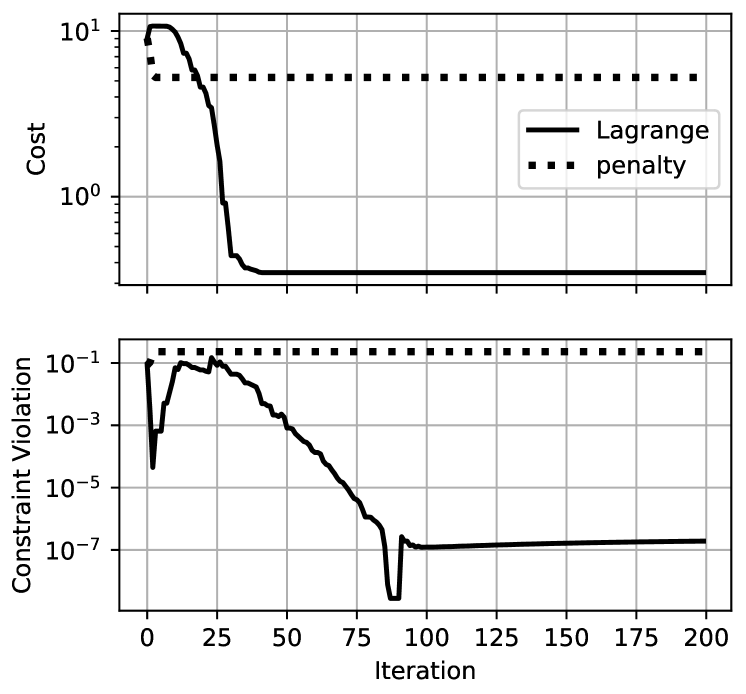
(a) Spinner

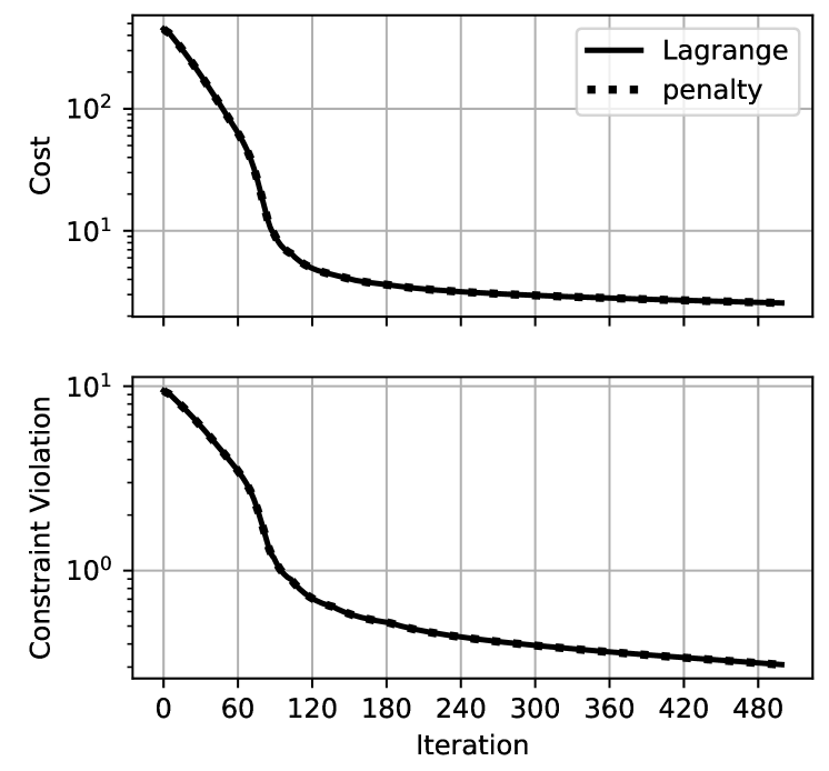
(b) Quadruped

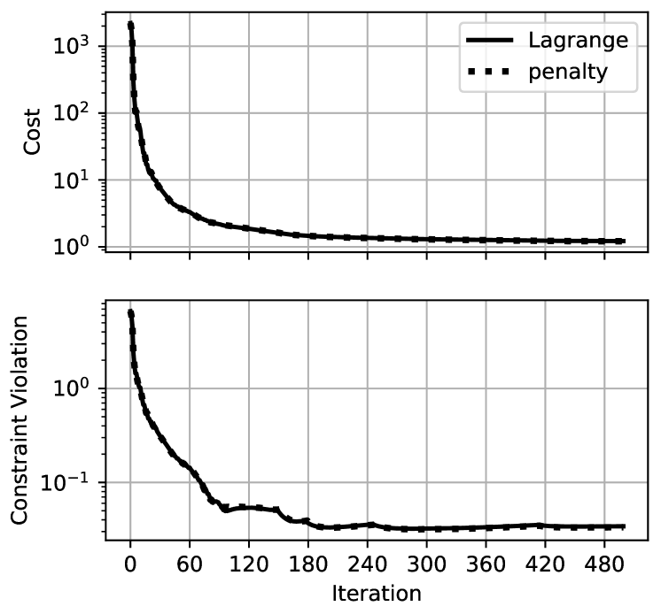
(c) Dual-Arm

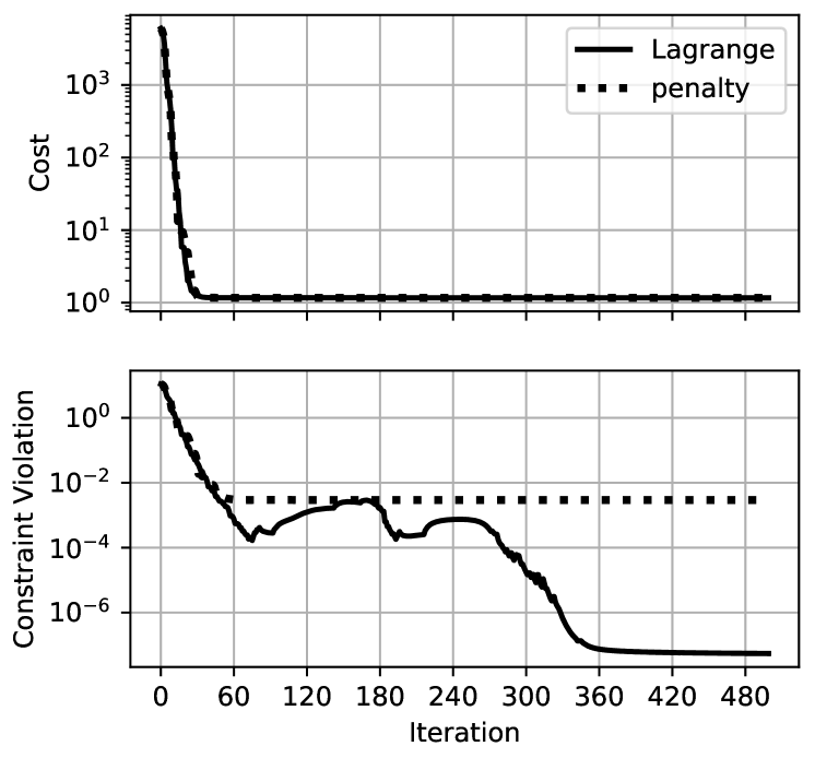
(d) Allegro Hand

Figure 3: Convergence with quadratic penalty and Lagrange multipliers for each of the four examples.

The LM method sometimes performed much better than the penalty method (spinner and Allegro hand), and occasionally found higher-quality local minima. This is shown in the spinner example, where the penalty was not able to drive the finger to touch the spinner, leading to a high cost and large constraint violations.

For the quadruped and bi-manual manipulation cases, the two methods produced nearly identical results. In these cases, the penalty method is preferable due to the cost of solving $\bm{\lambda}$ from (17). This additional cost is illustrated in Fig. 4, which plots the average wall-clock time per iteration for different planning horizons. With the penalty method, complexity is linear in the planning horizon and cubic in the number of DoFs, similar to iLQR/DDP. Scalability is worse with the LM method: our current implementation solves (17) using dense algebra, rendering complexity cubic in the planning horizon.

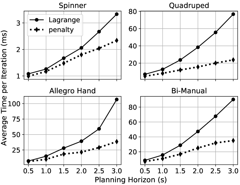
Figure 4: Average wall-clock time per iteration for various planning horizons. All examples used a 50 ms time step, with cost and gradient computations parallelized across 4 threads.

We emphasize that the convergence shown in Fig. 3 is not particularly good: for many of the examples, constraint violations are still large and the cost is still slowly decreasing even after 500 iterations. However, we found these solutions to be informative in offline CITO computations, particularly with the quick user interaction cycles enabled by the speed of these computations. For MPC, we found that high control rates compensate for poor convergence accuracy.

Figure 5 shows a breakdown of the computational cost, using a 2 s (40 step) horizon for all of the examples. Inverse dynamics derivatives (orange) are the most expensive component. Fortunately, derivatives and cost calculations are easily parallelized.

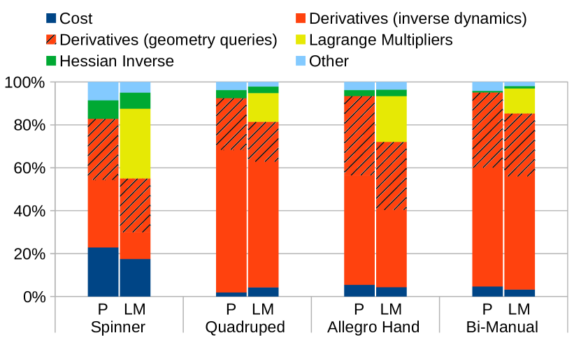
Figure 5: Percent of CPU time dedicated to major computational elements, using the penalty method (P) or Lagrange multipliers (LM) to handle equality constraints. Derivative and cost calculations (blue, orange, striped orange) can be trivially parallelized.

VI-D Model Predictive Control

We applied our solver to CI-MPC for all four example scenarios. As suggested by [27], we did not run the solver to convergence, but rather performed a single iteration before returning the solution. We then warm-started each subsequent solve from the previous solution.

Between iterations, we tracked the latest solution with a higher-frequency feed-forward PD controller,

$$\bm{u}=\bm{u}_{ff}+\bm{K}_{P}(\bm{q}_{d}-\hat{\bm{q}})+\bm{K}_{D}(\bm{v}_{d}-\hat{\bm{v}}),$$ (26)

where feedforward torques $\bm{u}_{ff}$, desired positions $\bm{q}_{d}$, and desired velocities $\bm{v}_{d}$ were obtained from a cubic spline interpolation of IDTO solutions, with the latest solution as the knot points. $\hat{\bm{q}}$ and $\hat{\bm{v}}$ are state estimates, and $\bm{K}_{P}$ and $\bm{K}_{D}$ are gain matrices.

VI-D1 Spinner

The goal is to move the spinner 2 radians past its starting position. For MPC, the starting position was constantly updated to match the current position, such that the spinner keeps spinning. Damping in the spinner joint means that the robot must constantly interact with the spinner to accomplish this task.

With the LM method and parallelization across 4 threads on a laptop (Intel i7-6820HQ, 32 GB RAM), MPC ran in real time at about 200 Hz. A “finger gaiting” cycle emerged from the optimization, as shown in the accompanying video. While the optimizer’s contact model allows some force at a distance, simulations with Drake’s contact model did not [33].

The spinner is inspired by an example in [2], which reports around 30 seconds of offline computation to generate similar behavior.

VI-D2 Mini Cheetah Quadruped

As for the spinner, we updated the quadruped’s goal at each iteration to move the robot forward at about 0.4 m/s. Again, while the planner’s compliant contact model allows force at a distance and included very large friction regularization, the simulator used Drake’s contact model with tight regularization of friction, physics-based compliance, and no action at a distance.

With the penalty method and parallelization across 4 threads on a laptop, MPC ran in real time at about 60 Hz. Over flat portions of the terrain, a trot-like gait emerged, with opposite pairs of legs working together. The robot deviated from this gait to cross two small hills. Screenshots from the generated trajectory are shown in Fig. 6, and the full simulation is shown in the supplemental video.

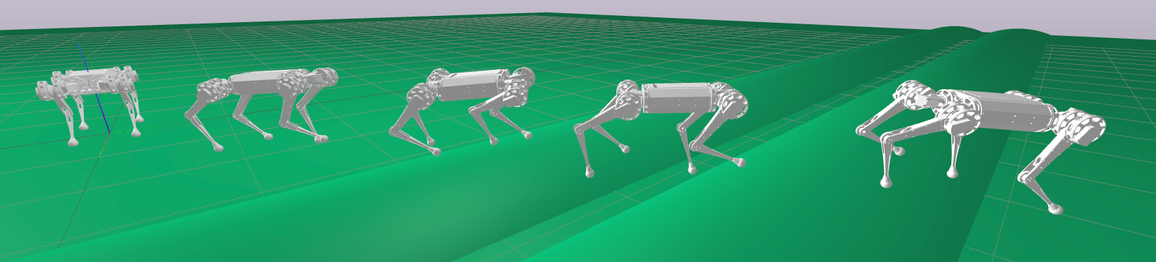
Figure 6: A simulated Mini Cheetah quadruped traverses two small hills. The simulation runs in real time while IDTO acts as an MPC controller at about 60 Hz. We do not specify a preferred contact sequence, only a quadratic cost defining the desired direction of travel. Nonetheless, a trot-like gait emerges in the flat sections.

VI-D3 Allegro Dexterous Hand

The robot was to rotate the ball 180 degrees in its hand. Unlike IDTO’s point contact, the simulation used a hydroelastic model of surface patches [44, 45] to simulate the rich interactions between the hand and the ball.

We found that the LM method was essential to obtaining good performance. With parallelization across 4 threads on a laptop, MPC ran in real time at 10 Hz. We found that the robot could perform different rotations merely by changing the desired orientation: no further parameter tuning was needed.

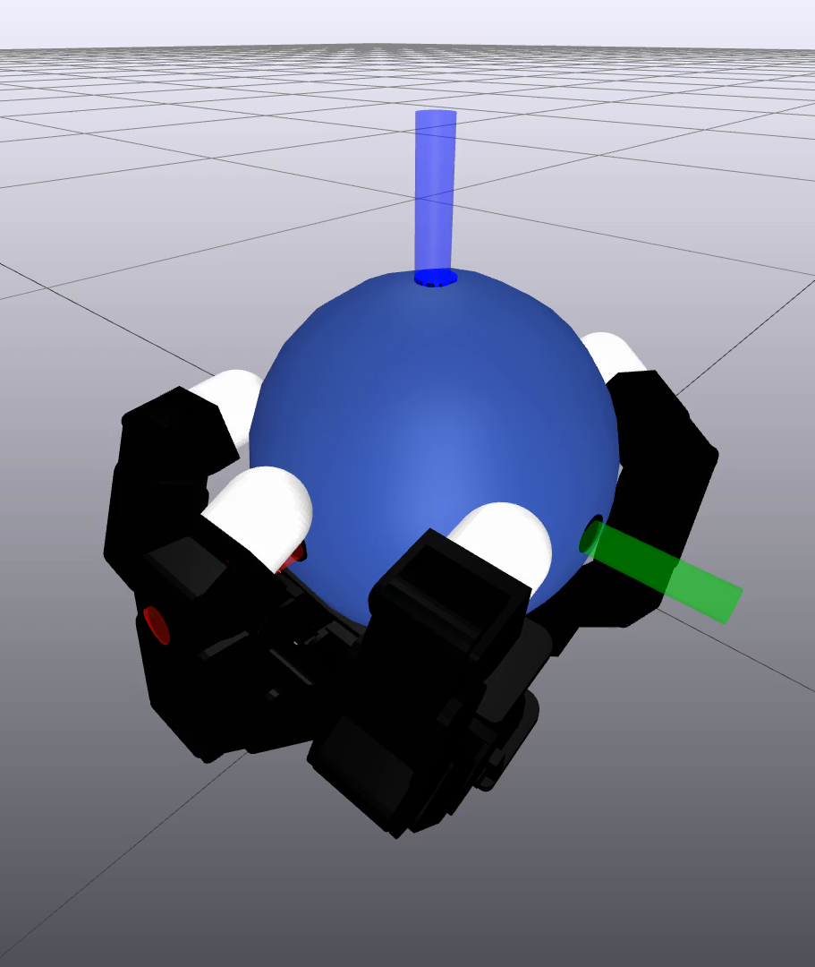
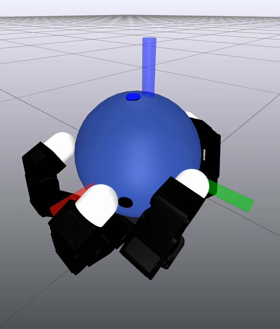
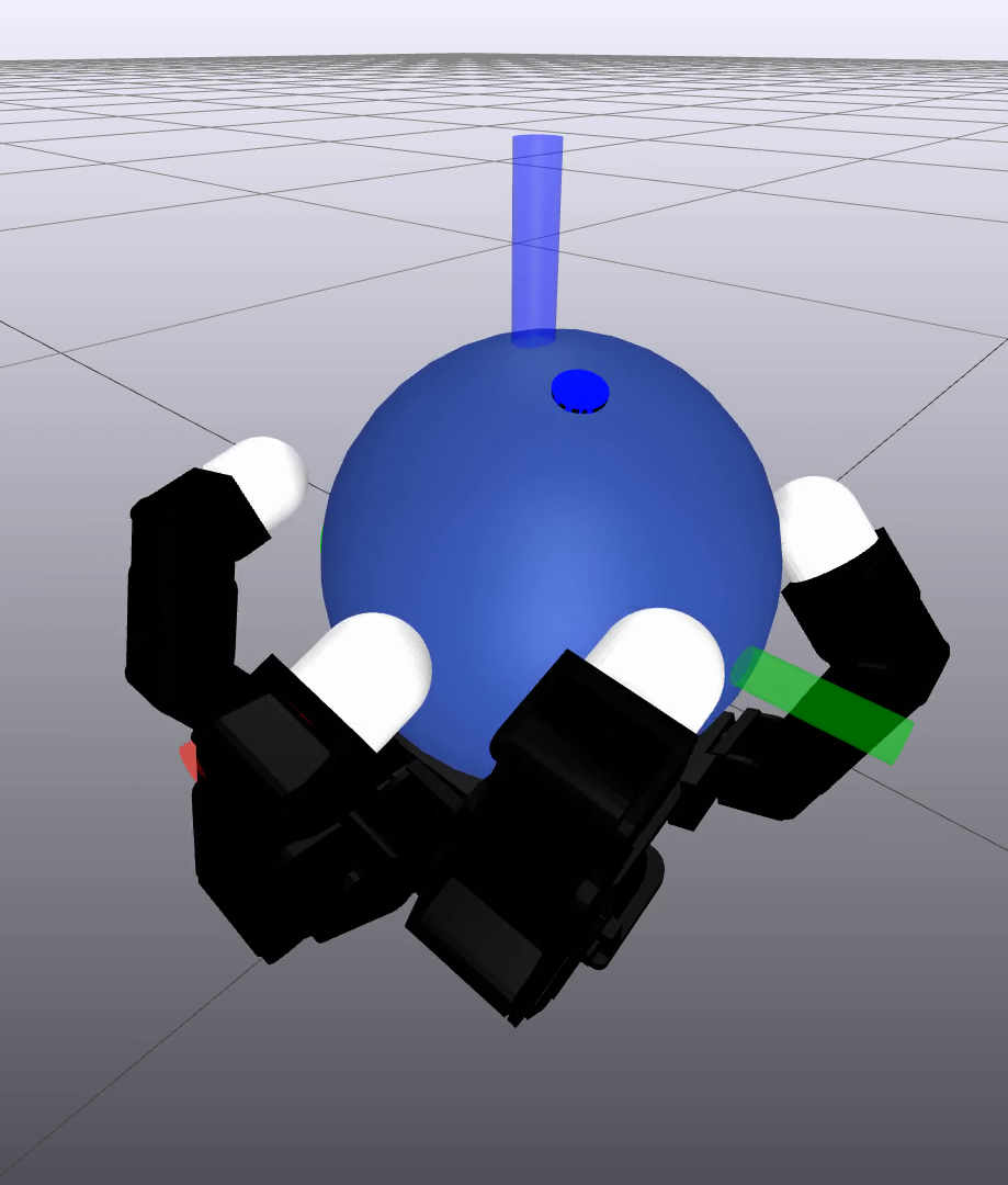
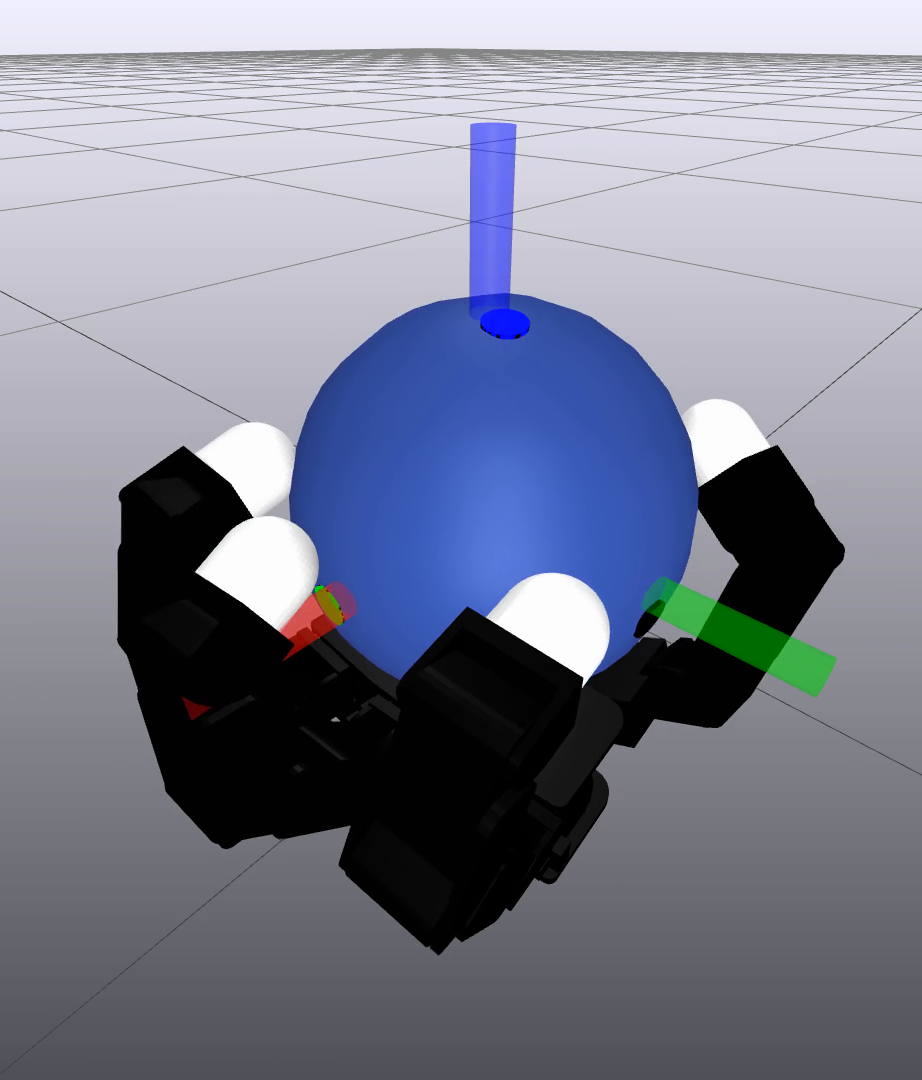
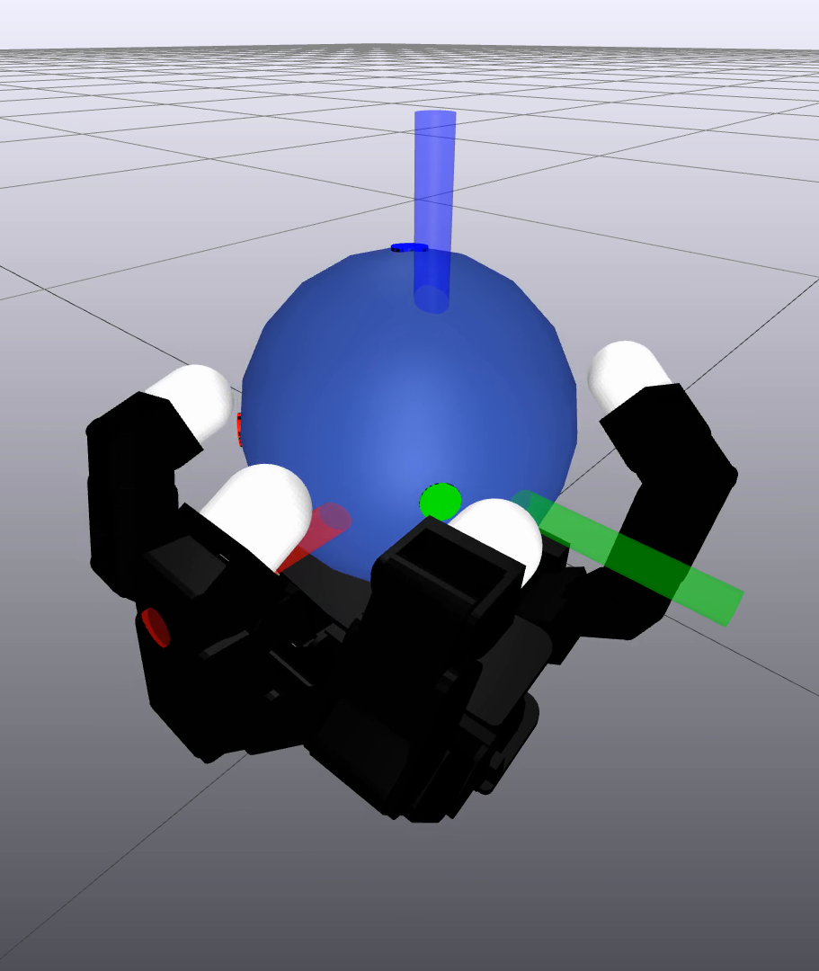
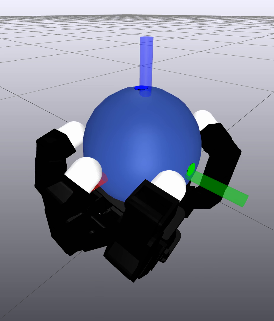
Figure 7: A simulated Allegro dexterous hand rotates a sphere 180 degrees. IDTO determines when and where to make and break contact at about 10 Hz. The planner uses the simple point contact model described in Section IV-B, while the simulator uses a hydroelastic model based on contact patches rather than contact points [44, 45].

The robot completed the 180-degree rotation shown in Fig. 7 in about 15 seconds, without any offline computation. The resulting trajectory is comparable to that obtained by [34], which uses a quasi-dynamic model and requires around a minute of offline compute to perform a similar 180-degree in-hand rotation.

VI-D4 Bi-Manual Manipulator

Finally, we validated our approach on hardware with two Jaco arms. We first designed several behaviors—push a box on the ground, pick up the box, and balance the box on its edge—in simulation. We used hydroelastic contact for the simulation, and ran MPC at around 15 Hz on a laptop.

For the hardware experiments, we used a system with a 24-core processor (AMD Ryzen Threadripper 3960x, 64 GB RAM). We parallelized derivative computations across 20 threads (one per time step). Together with the fact that the computer did not need to simultaneously run a simulation, this allowed us to perform MPC between 100-200 Hz. The exact rate varied through the experiments, depending on the contact configuration.

With a few exceptions, we used the same contact parameters in simulation and on hardware. The exceptions primarily had to do with friction, since we did not have accurate friction measurements available. We also used a larger friction coefficient (1.0 rather than 0.2) for the planner in the lifting task, as this encouraged the robot to squeeze the box more gently, and we wanted to push the box out of the robot’s grasp, as shown in Fig. 8.

The hardware setup differed slightly from that of the simulation. We operated the robot in position-control mode using Jaco’s proprietary controller with default gains. For the box, an Optitrack motion capture system measured pose, and we assumed zero velocity.

Footage of the hardware experiments can be found in the accompanying video. Screenshots of the picking-up task are shown in Fig. 8. These experiments highlight the usefulness of CI-MPC: our solver was able to recover from significant external disturbances, making and breaking contact, changing between sticking and sliding modes, and adjusting contact configurations on the fly.

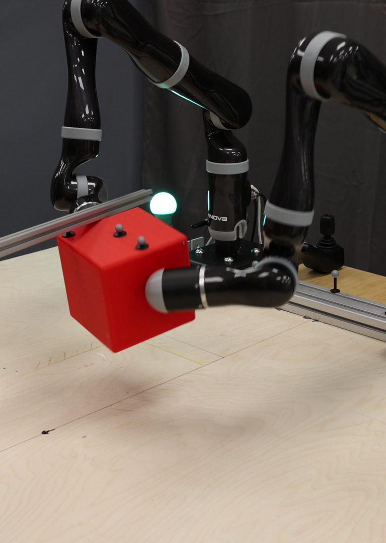
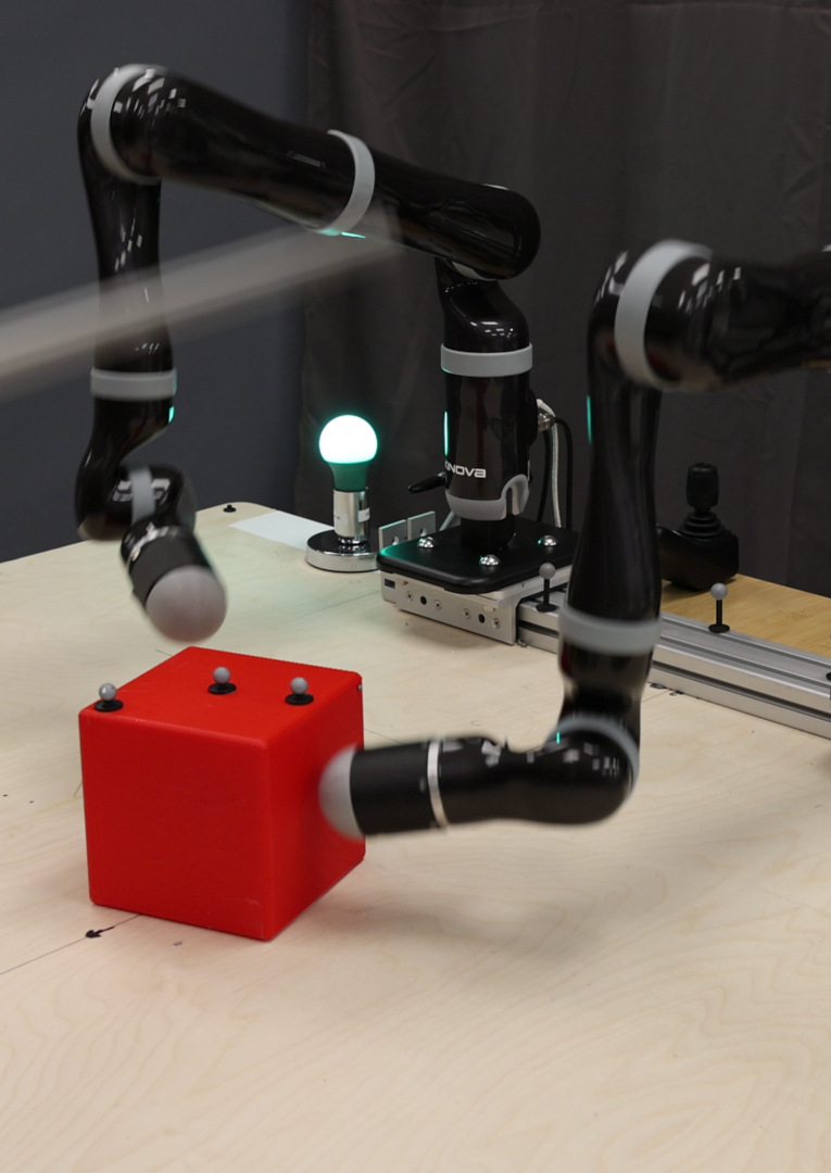
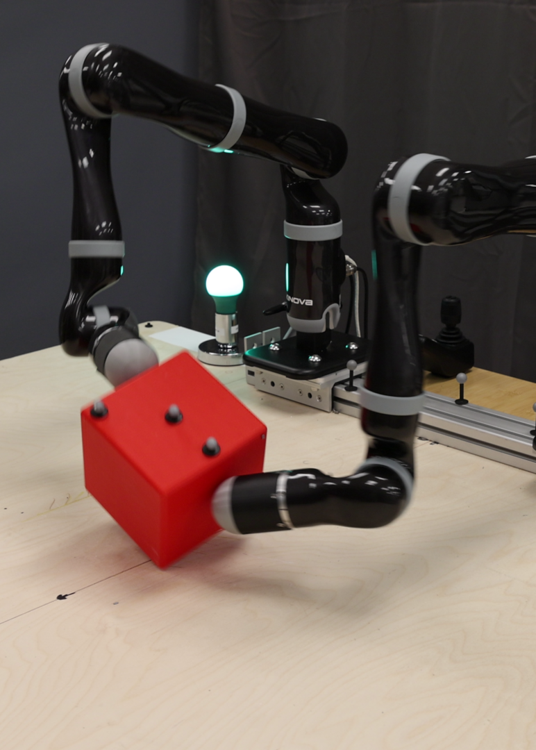
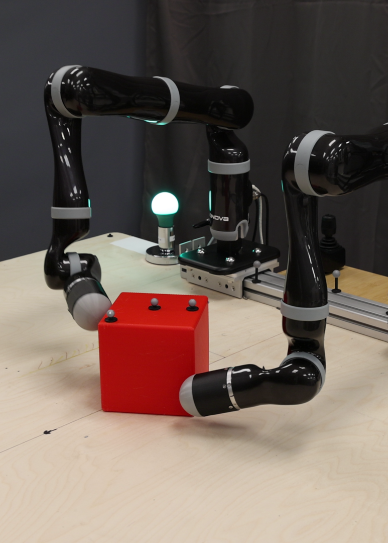
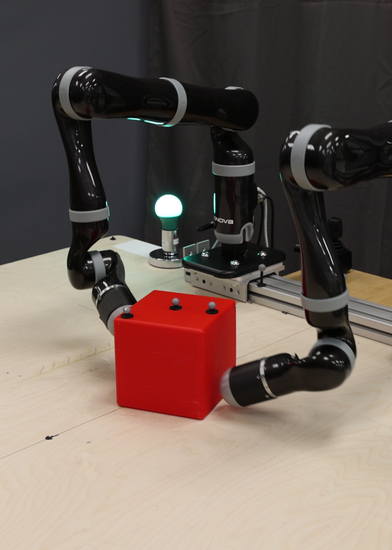
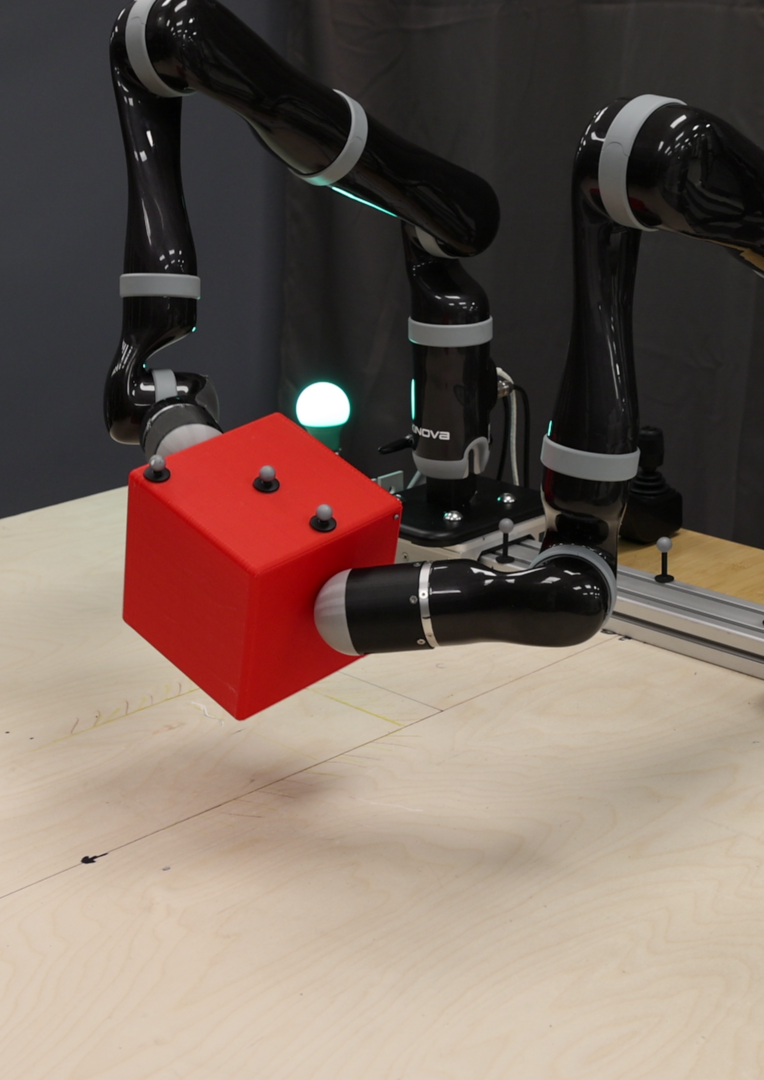
Figure 8: Two 7-DoF Kinova Jaco arms tasked with lifting a box recover from an external disturbance (push with a stick from above). After dropping the box, the robot attempts to re-grasp, but fails. The robot then selects a new contact configuration and succeeds on the second attempt.

Our experiments also illustrate some limitations of IDTO, particularly with respect to local minima. This is especially evident in the pushing example, where the robot is tasked with pushing the box on the table to a desired pose. The robot responds quickly and effectively to small disturbances, but is not able to recover from a large disturbance that takes the box far from the arms. With the box far away, there are no gradients that indicate to the solver that the arms should reach around the box to push it back: the system is stuck in a local minimum where the arms do not move.

The severity of such local minima can be reduced by increasing the smoothing parameter $\sigma$, but there is a tradeoff: with a very large $\sigma$ the planner expects a considerable amount of force at a distance, and may fail to actually make contact. A more problem-specific solution would be to add cost terms that encourage the end-effector to move to the side of the manipuland opposite the target pose [8].

VII Comparison with Existing Work

Table III compares IDTO to results reported in the literature. Due to space constraints, we focus on recent results that run CI-MPC in real time. We encourage the reader to read the cited references for further details. Notice that the oldest work is from 2018, with most from 2022 or newer, so major performance differences cannot be attributed to differences in processing power.

[b] Method System DoFs Horizon (s) $\delta t$ (s) MPC Iters. Freq. Simplified Dynamics Pref. Contact Sequence Hardware Neunert ’18 [27] Quadruped 18 0.5 0.004 1 190 Hz No Yes Yes Kong ’22 [16] Quadruped 18 0.5 0.01 1 ? No Yes Yes Howell ’22 [28] Quadruped 18 0.25 0.01 N/A¹ 100 Hz No Yes No Howell ’22 [28] Shadow Hand 26 0.25 0.01 N/A¹ 100 Hz No No No Le Cleach’h ’23 [9] Push Bot 2 1.6 0.04 ? 70 Hz No No No Le Cleach’h ’23 [9] Quadruped 18 0.15 0.05 ? 100 Hz Yes Yes Yes Aydinoglu ’23 [8] Finger Pivot 5 0.1 0.01 5 45 Hz No No No Aydinoglu ’23 [8] Ball Roll 9 0.5 0.1 2 80 Hz Yes No Yes Park ’23 [46] Quadruped 18 0.5 0.025 ? 40 Hz No Yes Yes IDTO (ours) Spinner 3 2.0 0.05 1 200 Hz No No No IDTO (ours) Hopper 5 2.0 0.05 1 100 Hz No No No IDTO (ours) Quadruped 18 1.0 0.05 1 60 Hz No No No IDTO (ours) Bi-Manual 20 1.0 0.05 1 100 Hz No No Yes IDTO (ours) Allegro Hand 22 2.0 0.05 1 10 Hz No No No

TABLE III: Comparison with real-time CI-MPC in the literature. Data marked with ? was not reported.

• We cannot talk about iterations for predictive sampling.

Nonetheless, hardware and software quality do significantly impact performance, and most methods in Table III would perform better with further optimization. This includes our own approach: while Drake is currently undergoing significant performance improvements, IDTO would benefit from faster multibody algebra. For example, MuJoCo can simulate a humanoid with 4000 timesteps per second on a single CPU [28]. By contrast, Drake runs a comparably sized model at around 800 timesteps per second.

Table III shows that IDTO allows longer planning horizons than many existing methods, a fact that is enabled by relatively large time steps. We do not simplify the system dynamics, though we do simplify collision geometries (see Remark 3). We are particularly proud of the fact that IDTO does not require a preferred contact sequence for the quadruped example, though specifying one is possible in the IDTO framework and might improve performance in practice.

VIII Limitations

In this section, we highlight the weaknesses of our approach, with an eye toward future CI-MPC research.

First, IDTO only guarantees dynamic feasibility at convergence due to the constraint (13b). In practice, non-converged solutions include forces on unactuated DoFs. For example, the spinner might spin without anything pushing it. With the quadratic penalty method these non-physical forces can exist even at convergence. The LM method helps, but does not mitigate the problem completely. In particular, LM is more costly than the penalty method and reduces the impact of parallelization (Fig. 5). Furthermore, equality constraints are still only enforced at convergence. Performance of LM could be improved with the use of sparse algebra in the computation of (17).

Solver convergence can be slow, as shown in Fig. 3. This is an inevitable result of the Gauss-Newton approximation — problem (13) is a large-residual problem, for which Gauss-Newton methods converge linearly [37]. Accelerating convergence with second-order techniques is a potentially fruitful area for future research.

Our solver does not currently support arbitrary constraints, such as input torque or joint angle limits. While approximating such constraints with a penalty method would be straightforward, this may not be suitable for athletic behaviors at the limit of a robot’s capabilities.

Computationally, the biggest bottleneck is computing derivatives. This is shown in orange and striped orange in Fig. 5. Recent advances in analytical derivatives of rigid-body dynamics algorithms [40, 47] could potentially alleviate this bottleneck, but such results would first need to be extended to include differentiation through contact.

Practically, our solver’s reliance on spherical collision geometries, as discussed in Remark 3, presents a major limitation. While inscribed spheres enabled basic box manipulation on hardware, this approximation introduces modeling errors that could be problematic for more complex tasks. A better long-term solution could be a model like hydroelastics [44, 45] that avoids discontinuous artifacts for objects with sharp edges.

As for most CITO solvers, cost weights and contact parameters determine IDTO’s performance in practice. While we found that IDTO was not particularly sensitive to changes in the cost weights, as evidenced by the multiples of 10 in Table II, IDTO is sensitive to contact modeling parameters, particularly the smoothing factor and stiction velocity. Nonetheless, we found that a fast solver made contact parameter tuning easier. This could be further improved with a graphical interface [28].

Finally, IDTO is a fundamentally local optimization method and as such is vulnerable to local minima. A more systematic “virtual force” framework [24, 32] could help reduce the severity of these local minima.

IX Conclusion

IDTO is a simple but surprisingly effective tool for planning and control through contact. Even with a basic contact model and simple quadratic costs, IDTO enables real-time CI-MPC in simulation and on hardware, and is competitive with the state of the art.

Areas for future research include improving contact discovery with virtual forces, developing faster (analytical) derivatives for inverse dynamics with contact, considering convex contact models [22], and extracting a local feedback policy in the style of iLQR/DDP. Further improvements could stem from proper handling of $SE(3)$ structure in the dynamics and second-order methods for faster convergence. Finally, to mitigate the local nature of IDTO, our solver could be combined with a higher-level global planner based on sampling [34], graph search [48], learning [49], or combinatorial motion planning [50].

X Acknowledgements

Thanks to Sam Creasey for helping with the Jaco hardware, and Jarod Wilson for 3D printing parts.

Appendix A Computing the Hessian Approximation

As outlined in Section V-C, we compute a Gauss-Newton approximation of the Hessian. This approximation neglects second-order time derivatives of the inverse dynamics when propagating derivatives through (23).

Separating the weight matrix $\bm{Q}=\text{diag}([\bm{Q}_{\bm{q}}~{}\bm{Q}_{\bm{v}}])$ into position and velocity components and noting the symmetry of $\bm{H}$, we compute nonzero blocks as follows:

$$\bm{H}_{k,k-2}=\left[\frac{\partial\bm{\tau}_{k-1}}{\partial\bm{q}_{k-2}}\right]^{T}\bm{R}\frac{\partial\bm{\tau}_{k-1}}{\partial\bm{q}_{k}},$$

$$\bm{H}_{k,k-1}=\left[\frac{\partial\bm{v}_{t}}{\partial\bm{q}_{k-1}}\right]^{T}\bm{Q}_{\bm{v}}\frac{\partial\bm{v}_{t}}{\partial\bm{q}_{k}}\\ +\left[\frac{\partial\bm{\tau}_{k-1}}{\partial\bm{q}_{k-1}}\right]^{T}\bm{R}\frac{\partial\bm{\tau}_{k-1}}{\partial\bm{q}_{k}}+\left[\frac{\partial\bm{\tau}_{k}}{\partial\bm{q}_{k-1}}\right]^{T}\bm{R}\frac{\partial\bm{\tau}_{k}}{\partial\bm{q}_{k}},$$

$$\bm{H}_{k,k}=\bm{Q}_{\bm{q}}+\left[\frac{\partial\bm{v}_{t}}{\partial\bm{q}_{t}}\right]^{T}\bm{Q}_{\bm{v}}\frac{\partial\bm{v}_{t}}{\partial\bm{q}_{t}}+\left[\frac{\partial\bm{v}_{k+1}}{\partial\bm{q}_{t}}\right]^{T}\bm{Q}_{\bm{v}}\frac{\partial\bm{v}_{k+1}}{\partial\bm{q}_{t}}+\\ \left[\frac{\partial\bm{\tau}_{k-1}}{\partial\bm{q}_{t}}\right]^{T}\bm{R}\frac{\partial\bm{\tau}_{k-1}}{\partial\bm{q}_{k}}+\left[\frac{\partial\bm{\tau}_{k}}{\partial\bm{q}_{t}}\right]^{T}\bm{R}\frac{\partial\bm{\tau}_{k}}{\partial\bm{q}_{k}}+\left[\frac{\partial\bm{\tau}_{k+1}}{\partial\bm{q}_{t}}\right]^{T}\bm{R}\frac{\partial\bm{\tau}_{k+1}}{\partial\bm{q}_{k}}.$$

Constructing this Hessian approximation requires only velocity and inverse dynamics derivatives — $\frac{\partial\bm{v}_{k}}{\partial\bm{q}_{k}}$, $\frac{\partial\bm{v}_{k+1}}{\partial\bm{q}_{k}}$, $\frac{\partial\bm{\tau}_{k-1}}{\partial\bm{q}_{k}}$, $\frac{\partial\bm{\tau}_{k}}{\partial\bm{q}_{k}}$, and $\frac{\partial\bm{\tau}_{k+1}}{\partial\bm{q}_{k}}$ — as discussed in Section V-C. Our solver calculates these derivatives once per iteration and caches them for computational efficiency.

References

- [1] P. M. Wensing, M. Posa, Y. Hu, A. Escande, N. Mansard, and A. Del Prete, “Optimization-based control for dynamic legged robots,” arXiv preprint arXiv:2211.11644, 2022.
- [2] M. Posa and R. Tedrake, “Direct trajectory optimization of rigid body dynamical systems through contact,” in Algorithmic foundations of robotics. Springer, 2013, pp. 527–542.
- [3] Z. Manchester, N. Doshi, R. J. Wood, and S. Kuindersma, “Contact-implicit trajectory optimization using variational integrators,” The International Journal of Robotics Research, vol. 38, no. 12-13, pp. 1463–1476, 2019.
- [4] A. W. Winkler, C. D. Bellicoso, M. Hutter, and J. Buchli, “Gait and trajectory optimization for legged systems through phase-based end-effector parameterization,” IEEE Robotics and Automation Letters, vol. 3, no. 3, pp. 1560–1567, 2018.
- [5] A. Patel, S. L. Shield, S. Kazi, A. M. Johnson, and L. T. Biegler, “Contact-implicit trajectory optimization using orthogonal collocation,” IEEE Robotics and Automation Letters, vol. 4, no. 2, pp. 2242–2249, 2019.
- [6] J. Moura, T. Stouraitis, and S. Vijayakumar, “Non-prehensile planar manipulation via trajectory optimization with complementarity constraints,” in 2022 International Conference on Robotics and Automation (ICRA). IEEE, 2022, pp. 970–976.
- [7] M. Wang, A. Ö. Önol, P. Long, and T. Padır, “Contact-implicit planning and control for non-prehensile manipulation using state-triggered constraints,” in Robotics Research. Springer, 2023, pp. 189–204.
- [8] A. Aydinoglu, A. Wei, and M. Posa, “Consensus complementarity control for multi-contact mpc,” arXiv preprint arXiv:2304.11259, 2023.
- [9] S. L. Cleac’h, T. Howell, M. Schwager, and Z. Manchester, “Fast contact-implicit model-predictive control,” arXiv preprint arXiv:2107.05616, 2023.
- [10] Y. Tassa, T. Erez, and E. Todorov, “Synthesis and stabilization of complex behaviors through online trajectory optimization,” in 2012 IEEE/RSJ International Conference on Intelligent Robots and Systems. IEEE, 2012, pp. 4906–4913.
- [11] M. Neunert, F. Farshidian, A. W. Winkler, and J. Buchli, “Trajectory optimization through contacts and automatic gait discovery for quadrupeds,” IEEE Robotics and Automation Letters, vol. 2, no. 3, pp. 1502–1509, 2017.
- [12] J. Carius, R. Ranftl, V. Koltun, and M. Hutter, “Trajectory optimization with implicit hard contacts,” IEEE Robotics and Automation Letters, vol. 3, no. 4, pp. 3316–3323, 2018.
- [13] I. Chatzinikolaidis and Z. Li, “Trajectory optimization of contact-rich motions using implicit differential dynamic programming,” IEEE Robotics and Automation Letters, vol. 6, no. 2, pp. 2626–2633, 2021.
- [14] G. Kim, D. Kang, J.-H. Kim, and H.-W. Park, “Contact-implicit differential dynamic programming for model predictive control with relaxed complementarity constraints,” in 2022 IEEE/RSJ International Conference on Intelligent Robots and Systems (IROS). IEEE, 2022, pp. 11 978–11 985.
- [15] T. A. Howell, S. Le Cleac’h, S. Singh, P. Florence, Z. Manchester, and V. Sindhwani, “Trajectory optimization with optimization-based dynamics,” IEEE Robotics and Automation Letters, vol. 7, no. 3, pp. 6750–6757, 2022.
- [16] N. J. Kong, C. Li, and A. M. Johnson, “Hybrid iLQR model predictive control for contact implicit stabilization on legged robots,” arXiv preprint arXiv:2207.04591, 2022.
- [17] T. Erez and E. Todorov, “Trajectory optimization for domains with contacts using inverse dynamics,” in 2012 IEEE/RSJ International Conference on Intelligent Robots and Systems. IEEE, 2012, pp. 4914–4919.
- [18] E. Todorov, “Acceleration based methods,” 2019, https://youtu.be/uWADBSmHebA.
- [19] M. Posa, S. Kuindersma, and R. Tedrake, “Optimization and stabilization of trajectories for constrained dynamical systems,” in 2016 IEEE International Conference on Robotics and Automation (ICRA). IEEE, 2016, pp. 1366–1373.
- [20] D. Mayne, “A second-order gradient method for determining optimal trajectories of non-linear discrete-time systems,” International Journal of Control, vol. 3, no. 1, pp. 85–95, 1966.
- [21] W. Li and E. Todorov, “Iterative linear quadratic regulator design for nonlinear biological movement systems.” in ICINCO (1). Citeseer, 2004, pp. 222–229.
- [22] A. M. Castro, F. N. Permenter, and X. Han, “An unconstrained convex formulation of compliant contact,” IEEE Transactions on Robotics, vol. 39, no. 2, pp. 1301–1320, 2022.
- [23] A. Ö. Önol, P. Long, and T. Padır, “Contact-implicit trajectory optimization based on a variable smooth contact model and successive convexification,” in 2019 International Conference on Robotics and Automation (ICRA). IEEE, 2019, pp. 2447–2453.
- [24] A. Ö. Önol, R. Corcodel, P. Long, and T. Padır, “Tuning-free contact-implicit trajectory optimization,” in 2020 IEEE International Conference on Robotics and Automation (ICRA). IEEE, 2020, pp. 1183–1189.
- [25] H. J. T. Suh, T. Pang, and R. Tedrake, “Bundled gradients through contact via randomized smoothing,” IEEE Robotics and Automation Letters, vol. 7, no. 2, pp. 4000–4007, 2022.
- [26] M. Giftthaler, M. Neunert, M. Stäuble, J. Buchli, and M. Diehl, “A family of iterative gauss-newton shooting methods for nonlinear optimal control,” in 2018 IEEE/RSJ International Conference on Intelligent Robots and Systems (IROS). IEEE, 2018, pp. 1–9.
- [27] M. Neunert, M. Stäuble, M. Giftthaler, C. D. Bellicoso, J. Carius, C. Gehring, M. Hutter, and J. Buchli, “Whole-body nonlinear model predictive control through contacts for quadrupeds,” IEEE Robotics and Automation Letters, vol. 3, no. 3, pp. 1458–1465, 2018.
- [28] T. Howell, N. Gileadi, S. Tunyasuvunakool, K. Zakka, T. Erez, and Y. Tassa, “Predictive sampling: Real-time behaviour synthesis with mujoco,” arXiv preprint arXiv:2212.00541, 2022.
- [29] H. Ferrolho, V. Ivan, W. Merkt, I. Havoutis, and S. Vijayakumar, “Inverse dynamics vs. forward dynamics in direct transcription formulations for trajectory optimization,” in 2021 IEEE International Conference on Robotics and Automation (ICRA). IEEE, 2021, pp. 12 752–12 758.
- [30] I. Mordatch, Z. Popović, and E. Todorov, “Contact-invariant optimization for hand manipulation,” in Proceedings of the ACM SIGGRAPH/Eurographics symposium on computer animation, 2012, pp. 137–144.
- [31] I. Mordatch, E. Todorov, and Z. Popović, “Discovery of complex behaviors through contact-invariant optimization,” ACM Transactions on Graphics (TOG), vol. 31, no. 4, pp. 1–8, 2012.
- [32] E. Todorov, “Optico: A framework for model-based optimization with mujoco physics,” Invited Talk, Neural Information Processing Systems, 2019, https://slideslive.com/38922729/.
- [33] A. M. Castro, A. Qu, N. Kuppuswamy, A. Alspach, and M. Sherman, “A transition-aware method for the simulation of compliant contact with regularized friction,” IEEE Robotics and Automation Letters, vol. 5, no. 2, pp. 1859–1866, 2020.
- [34] T. Pang, H. T. Suh, L. Yang, and R. Tedrake, “Global planning for contact-rich manipulation via local smoothing of quasi-dynamic contact models,” IEEE Transactions on Robotics, 2023.
- [35] K. Hunt and F. Crossley, “Coefficient of restitution interpreted as damping in vibroimpact,” Journal of Applied Mechanics, vol. 42, no. 2, pp. 440–445, 1975.
- [36] J. J. Moré, “The levenberg-marquardt algorithm: implementation and theory,” in Numerical analysis: proceedings of the biennial Conference held at Dundee, June 28–July 1, 1977. Springer, 2006, pp. 105–116.
- [37] J. Nocedal and S. J. Wright, Numerical optimization, 2nd ed. New York: Springer, 2006.
- [38] K. Benkert and R. Fischer, “An efficient implementation of the thomas-algorithm for block penta-diagonal systems on vector computers,” in International Conference on Computational Science. Springer, 2007, pp. 144–151.
- [39] J. Carpentier and N. Mansard, “Analytical derivatives of rigid body dynamics algorithms,” in Robotics: Science and systems (RSS 2018), 2018.
- [40] S. Singh, R. P. Russell, and P. M. Wensing, “Efficient analytical derivatives of rigid-body dynamics using spatial vector algebra,” IEEE Robotics and Automation Letters, vol. 7, no. 2, pp. 1776–1783, 2022.
- [41] L. Cui and J. Dai, “Geometric kinematics of rigid bodies with point contact,” in Advances in Robot Kinematics: Motion in Man and Machine: Motion in Man and Machine. Springer, 2010, pp. 429–436.
- [42] E. G. Gilbert, D. W. Johnson, and S. S. Keerthi, “A fast procedure for computing the distance between complex objects in three-dimensional space,” IEEE Journal on Robotics and Automation, vol. 4, no. 2, pp. 193–203, 1988.
- [43] B. Katz, J. Di Carlo, and S. Kim, “Mini cheetah: A platform for pushing the limits of dynamic quadruped control,” in 2019 international conference on robotics and automation (ICRA). IEEE, 2019, pp. 6295–6301.
- [44] R. Elandt, E. Drumwright, M. Sherman, and A. Ruina, “A pressure field model for fast, robust approximation of net contact force and moment between nominally rigid objects,” in 2019 IEEE/RSJ International Conference on Intelligent Robots and Systems (IROS). IEEE, 2019, pp. 8238–8245.
- [45] J. Masterjohn, D. Guoy, J. Shepherd, and A. Castro, “Velocity level approximation of pressure field contact patches,” IEEE Robotics and Automation Letters, vol. 7, no. 4, pp. 11 593–11 600, 2022.
- [46] H.-W. Park, “Model predictive control for legged robots,” 2023, seminar, IEEE RAS Technical Committee on Model Based Optimization for Robotics. [Online]. Available: https://youtu.be/ivfQNhxEjAw
- [47] J. Carpentier, G. Saurel, G. Buondonno, J. Mirabel, F. Lamiraux, O. Stasse, and N. Mansard, “The pinocchio c++ library: A fast and flexible implementation of rigid body dynamics algorithms and their analytical derivatives,” in 2019 IEEE/SICE International Symposium on System Integration (SII). IEEE, 2019, pp. 614–619.
- [48] R. Natarajan, G. L. Johnston, N. Simaan, M. Likhachev, and H. Choset, “Torque-limited manipulation planning through contact by interleaving graph search and trajectory optimization,” in 2023 IEEE International Conference on Robotics and Automation (ICRA), 2023.
- [49] C. Chi, S. Feng, Y. Du, Z. Xu, E. Cousineau, B. Burchfiel, and S. Song, “Diffusion policy: Visuomotor policy learning via action diffusion,” arXiv preprint arXiv:2303.04137, 2023.
- [50] T. Marcucci, J. Umenberger, P. A. Parrilo, and R. Tedrake, “Shortest paths in graphs of convex sets,” arXiv preprint arXiv:2101.11565, 2021.