Neural-Singular-Hessian: Implicit Neural Representation of Unoriented Point Clouds by Enforcing Singular Hessian

Abstract.

Neural implicit representation is a promising approach for reconstructing surfaces from point clouds. Existing methods combine various regularization terms, such as the Eikonal and Laplacian energy terms, to enforce the learned neural function to possess the properties of a Signed Distance Function (SDF). However, inferring the actual topology and geometry of the underlying surface from poor-quality unoriented point clouds remains challenging. In accordance with Differential Geometry, the Hessian of the SDF is singular for points within the differential thin-shell space surrounding the surface. Our approach enforces the Hessian of the neural implicit function to have a zero determinant for points near the surface. This technique aligns the gradients for a near-surface point and its on-surface projection point, producing a rough but faithful shape within just a few iterations. By annealing the weight of the singular-Hessian term, our approach ultimately produces a high-fidelity reconstruction result. Extensive experimental results demonstrate that our approach effectively suppresses ghost geometry and recovers details from unoriented point clouds with better expressiveness than existing fitting-based methods.

Figure 1. Starting with an unoriented point cloud (left), our approach proposes an implicit neural representation by enforcing the Hessian of the implicit function to be singular for points in close proximity to the surface. By gradually reducing the weight of the singular-Hessian term, it works in a coarse-to-fine fashion and can ultimately produce a high-fidelity reconstruction result (right).

1. Introduction

In recent years, numerous learning-based approaches have been developed to recover the implicit representation of underlying surfaces from point clouds, a fundamental task in computer graphics and computer vision. Despite significant progress (Gropp et al., 2020; Sitzmann et al., 2020; Yifan et al., 2021; Xu et al., 2022) in surface reconstruction from high-quality point clouds with reliable normals, predicting a faithful surface from an unoriented point cloud remains a challenging and intriguing research problem due to the lack of sufficient geometric priors.

\begin{overpic}[width=433.62pt]{figures/top.pdf} \par\put(10.5,-3.0){PCP~{}\cite[citeyearpar]{(\@@bibref{Year}{PCP}{}{})}} \par\put(43.0,-3.0){DiGS~{}\cite[citeyearpar]{(\@@bibref{Year}{DiGS}{}{})}} \par\put(79.0,-3.0){{Ours}} \end{overpic}

Figure 2. Our approach can reconstruct rich geometric details from unoriented point clouds while PCP (Baorui et al., 2022b) and DiGS (Ben-Shabat et al., 2022) cannot.

Relevant research on reconstructing unoriented point clouds includes both traditional approaches (Hou et al., 2022; Lin et al., 2022) and learning-based approaches (Park et al., 2019; Mescheder et al., 2019; Songyou et al., 2020; Erler et al., 2020; Boulch and Marlet, 2022; Atzmon and Lipman, 2020; Baorui et al., 2021, 2022a, 2022b; Ben-Shabat et al., 2022). Traditional approaches typically involve repeatedly adjusting normals to be orthogonal to the zero isosurfaces of an implicit representation, such as a signed distance function (SDF) or an occupancy field. Learning-based approaches can be further categorized into supervised and fitting-based methods. Supervised learning approaches involve fitting data samples using ground-truth implicit representations as a guide (Park et al., 2019; Mescheder et al., 2019; Songyou et al., 2020; Erler et al., 2020; Boulch and Marlet, 2022). However, these approaches may not generalize well to shapes or point distributions not present in the training set (Sulzer et al., 2023). Fitting-based approaches (Atzmon and Lipman, 2020; Baorui et al., 2021, 2022a, 2022b; Ben-Shabat et al., 2022), instead, employ different combinations of regularization terms to ensure specific properties of a signed distance function (SDF) in order to solve an optimization problem for each input point cloud, such as the Eikonal term (Gropp et al., 2020) and the Laplacian energy term (Ben-Shabat et al., 2022). While these approaches have strong generalization capabilities, their performance may be compromised when normals are unavailable. Despite the use of the Eikonal term to suppress vanishing gradients, controlling the overall shape to adapt to the geometry and topology complexity of an input point cloud remains challenging. On the one hand, it is essential to accurately capture geometric details. On the other hand, unnecessary shape variations and ghost geometry must be eliminated.

In this paper, we address this problem based on the shape operator (O’Neill, 2006) from differential geometry. Given a smooth surface, there must exist a narrow thin-shell space surrounding it where the signed distance function (SDF) is differentiable everywhere. For a point $x$ in the thin-shell space whose projection onto the surface is $x^{\prime}$, the Hessian of the SDF at $x$ has three eigenvectors, two of which align with principal curvature directions at $x^{\prime}$, and the other aligns with normal vector at $x^{\prime}$ with a corresponding eigenvalue of zero, making the Hessian singular. In other words, by enforcing the Hessian to own a zero determinant for points near the surface, it helps align the gradient at $x$ with the normal vector at $x^{\prime}$. Based on this observation, we regularize the direction of the gradient of the SDF by enforcing the Hessian to own a zero determinant for points near the surface.

Making the Hessian singular differs from enforcing smoothness energy, such as Hessian energy (Calakli and Taubin, 2011; Zhang et al., 2022) or Laplacian energy (Ben-Shabat et al., 2022). The main difference is that the former can align the gradients of a near-surface point and its corresponding on-surface point, effectively suppressing surplus shape variations and adapting the implicit function to the inherent complexity of the input point cloud. Smoothness energy, on the other hand, tends to reduce the volatility of the implicit function so that the resulting surface is not overly complicated. Additionally, while the theoretical minimum value of smoothness energy cannot be zero (otherwise, the implicit function degenerates to a globally constant or linear field), the determinant of the Hessian of the implicit function can be reduced as far as possible. Finally, the singular-Hessian constraint can effectively eliminate critical points of the target implicit function near the surface and avoid unnecessary variations (e.g., ghost geometry). This can be explained by Morse theory (Audin et al., 2014), which reveals the deep link between the geometry and topology complexity of the surface and the number of critical points of the implicit function.

In implementation, we use sinusoidal activation (Sitzmann et al., 2020) to enable the computation of the first-order and the second-order derivatives of the implicit function. Our approach first generates a rough but faithful shape by emphasizing the singular-Hessian constraint and then anneals the constraint to gradually capture fine details and real topology in a coarse-to-fine fashion. Extensive experimental results demonstrate that our approach can eliminate ghost geometry while remaining expressive enough to recover geometric details and sharp features. Compared to state-of-the-art methods, our approach has superior performance in both fitting a single unoriented point cloud and learning a shape space from a group of point data. It can be seen from Fig. 2 that the reconstructed result by our approach has richer geometric details and higher fidelity than recently proposed methods such as PCP (Baorui et al., 2022b) and DiGS (Ben-Shabat et al., 2022).

2. Related Work

In recent decades, numerous surface reconstruction algorithms have been proposed (Jin et al., 2020; Huang et al., 2022b; Sulzer et al., 2023). While most existing research assumes the presence of normals, there has been growing interest in surface reconstruction from unoriented point clouds. This section provides an overview of implicit surface reconstruction methods, including both traditional and learning-based approaches.

2.1. Traditional Implicit Methods

The earliest implicit method computes the signed distance to the tangent plane of the closest point (Hoppe et al., 1992). After that, radial basis function (RBF) based methods (Carr et al., 2001; Li et al., 2016; Huang et al., 2019) represent the underlying SDF as a weighted combination of radial basis kernels, resulting in higher smoothness. Besides, the implicit moving least-square methods (IMLS) (Shen et al., 2004; Kolluri, 2008; Öztireli et al., 2009; Schroers et al., 2014) approximates the underlying SDF by linearly blending local smooth planes. The MPU method (Ohtake et al., 2003) models shape by blending piecewise quadratic functions that fit the local shape. Poisson reconstruction (Kazhdan et al., 2006) and its variants (Kazhdan et al., 2013, 2020; Vizzo et al., 2021; Sellán and Jacobson, 2022) formulate the occupancy field as the solution to Poisson’s equation. The SSD method (Calakli and Taubin, 2011) computes the smooth signed distance by minimizing least-square style energy with a multi-grid solver. Recently, iPSR (Hou et al., 2022) iteratively runs the Poisson reconstruction solver to produce a reconstructed surface from an unoriented point cloud, using the normals of the reconstructed surface from the previous iteration as input for the next iteration. PGR (Lin et al., 2022) infers the occupancy field based on Gauss’s formula in potential theory by considering surface element areas and normals as unknown parameters.

2.2. Learning-based Methods

Learning-based approaches can be further categorized into supervised and fitting-based methods, which are briefly introduced as follows.

Supervised Learning-based Reconstruction

Supervised learning-based reconstruction involves learning the SDF or occupancy field using a dataset containing precomputed ground-truth field values. The neural model adjusts its weights as input data is fed into it until the model is appropriately fitted. Thanks to the data prior provided by the ground-truth data, these methods generally produce impressive reconstruction results. Early works encode a global shape into a fixed-length latent code and recover the underlying surface through a decoding operation (Park et al., 2019; Mescheder et al., 2019). While these methods can encode the overall representation for a group of similar shapes, they struggle to generalize from training examples to unseen shapes and to encode shape details with the global code. To capture the richness of geometry for generality, some research subdivides 3D space according to surface occupancy and encodes each part separately, using voxel grid (Jiang et al., 2020; Chabra et al., 2020; Songyou et al., 2020), k-nearest neighbors (Erler et al., 2020; Boulch and Marlet, 2022), or octrees (Tang et al., 2021a; Wang et al., 2022; Huang et al., 2022a). In the context of open surface reconstruction (e.g., clothes), unsigned distance field (UDF) based surface reconstruction has attracted increasing attention in recent years (Chibane et al., 2020; Ye et al., 2022).

Fitting-based Implicit Neural Representation

To increase generalization ability, directly fitting the implicit representation from raw point clouds has been extensively studied in recent years, enabling end-to-end prediction of the target surface. Most methods apply different regularization techniques to accomplish this task. SAL/SALD (Atzmon and Lipman, 2020, 2021) performs sign agnostic regression to obtain a signed version from the unsigned distance function. IGR (Gropp et al., 2020) directly applies the Eikonal term to encourage the predicted implicit function to have unit gradients. Inspired by the definition of the SDF, Neural-Pull (Baorui et al., 2021) trains a neural network to predict the signed distance and gradients simultaneously so that a query point can be pulled to the closest point on the underlying surface. Based on Neural-Pull, PredictableContextPrior (Baorui et al., 2022b) first trains a local context prior and then specializes it in the predictive context prior to learning predictive queries at inference time. OnSurfacePrior (Baorui et al., 2022a) improves the reconstruction quality for sparse point clouds with the help of a pre-trained unsigned distance network. Recently, CAP-UDF (Zhou et al., 2022) extends Neural-Pull to learn UDFs directly from raw point clouds. SIREN (Sitzmann et al., 2020) shows that ReLU-MLPs bias toward low-frequency implicit representations, and then it introduces periodic activation functions to preserve high frequencies. Based on SIREN, Iso-Points (Yifan et al., 2020) constrains the hybrid representation grouped by explicit point clouds and implicit neural representation simultaneously to improve the reconstruction quality. DiGS (Ben-Shabat et al., 2022) incorporates Laplacian energy as a soft constraint of the SDF to enable unoriented point cloud reconstruction for SIREN. In general, most existing approaches require oriented normals to produce high-quality results. However, the absence of normals may compromise their performance, resulting in over-smoothed shapes lacking rich geometric details.

Figure 3. Visualizing the differential properties of an SDF for a circle. In contrast to the divergence of the gradient (i.e., Laplacian energy) utilized by (Ben-Shabat et al., 2022), the determinant of the Hessian matrix of the SDF remains consistently zero. This is due to the mathematical fact that, in the differentiable region near the surface, there exists a zero eigenvalue associated with an eigenvector aligned with the gradient.

3. PRELIMINARIES

Given an unoriented point cloud $\mathcal{P}$, our goal is to find an implicit representation ${f}:\mathbb{R}^{3}\mapsto\mathbb{R}$ such that the zero level set of ${f}$ accurately encodes the target surface $\mathcal{S}$:

(1) $$\mathcal{S}=\left\{\boldsymbol{x}\in\mathbb{R}^{3}\mid f(\boldsymbol{x})=0\right\}.$$

The discrete surface representation can be extracted from ${f}$ using contouring algorithms. It is important to note that our work requires $f$ to be $C^{2}$ continuous.

In previous research, it has been considered a suitable choice to encourage the neural implicit function $f$ to approximate the signed distance function (SDF). To achieve this, $f$ must satisfy three boundary conditions: (1) Dirichlet condition: $f(p)=0$ for $p\in\mathcal{P}$, which encourages any given point to lie on the target surface. (2) Eikonal condition: $\lVert\nabla f\rVert=1$, which enforces $f$ to have a unit gradient norm or, at the very least, not to vanish as much as possible. (3) Neumann condition: $\nabla f=\mathcal{N}$, which aligns the gradients with the normal field $\mathcal{N}$ if the normals are available. Existing implicit neural functions leverage the above boundary conditions as constraints, either explicitly (Gropp et al., 2020; Sitzmann et al., 2020) or implicitly (Baorui et al., 2021; Atzmon and Lipman, 2020). In this paper, our method leverages the same network architecture as SIREN (Sitzmann et al., 2020).

Figure 4. The illustration of the difference between the signed distance field and the relaxing signed distance field in terms of distance sign and gradient.

For the point cloud $\mathcal{P}$, let $\mathcal{Q}_{\text{far}}$ be a query point set uniformly sampled from its bounding box. SIREN formulates these requirements into loss terms as below.

(2) $$L_{\text{manifold}}=\int_{\mathcal{P}}\lVert f(x)\rVert_{1}dx$$

(3) $$L_{\text{non-manifold}}=\int_{\mathcal{Q}_{\text{far}}}\exp(-\alpha\lVert f(x)\rVert_{1})dx,\alpha=100$$

(4) $$L_{\text{Eikonal}}=\int_{\mathcal{P}\cup\mathcal{Q}_{\text{far}}}\lVert\lVert\nabla f(x)\rVert_{2}-1\rVert_{1}dx$$

(5) $$L_{\text{Neumann}}=\int_{\mathcal{P}}(1-\langle\nabla f(x),\mathcal{N}(x)\rangle)dx.$$

The overall loss is thus given by

(6) $$\begin{split}L^{\text{oriented}}_{\text{SIREN}}=&\lambda_{\text{manifold}}L_{\text{manifold}}+\lambda_{\text{non-manifold}}L_{\text{non-manifold}}+\\ &\lambda_{\text{Eikonal}}L_{\text{Eikonal}}+\lambda_{\text{Neumann}}L_{\text{Neumann}},\end{split}$$

where the four weights are respectively 3000, 100, 50, and 100. If the normals are not available, the loss reduces to

(7) $$\begin{split}L^{\text{unoriented}}_{\text{SIREN}}=&\lambda_{\text{manifold}}L_{\text{manifold}}+\lambda_{\text{non-manifold}}L_{\text{non-manifold}}+\\ &\lambda_{\text{Eikonal}}L_{\text{Eikonal}}.\end{split}$$

Despite the fact that the loss terms of SIREN establish meaningful constraints, optimizing SIREN presents a significant challenge. As indicated by IDF (Yifan et al., 2021), even when provided with normals, SIREN may generate numerous surplus parts. This problem is compounded when working with unoriented inputs. If the quality of the point cloud is poor, accurately estimating reliable normals or orientations can be notoriously difficult (Xu et al., 2023). In addressing the challenges associated with optimizing SIREN, it is important to recognize that there are an infinite number of candidate Eikonal solutions when enforcing the eikonal constraint at a limited number of sampled points, as discussed in DiGS (Ben-Shabat et al., 2022). Only eikonal constraint may result in the neural network optimization becoming trapped in a local minimum with the emergence of ghost geometry, which is far removed from the optimal solution. Additionally, over-parametrized neural networks (Sagun et al., 2017) often possess a large number of parameters, which can further complicate the optimization process. Some approaches employ a form of smoothness energy, such as Dirichlet energy (Lipman, 2021), Laplacian energy (Ben-Shabat et al., 2022) and Hessian energy (Calakli and Taubin, 2011; Schroers et al., 2014; Zhang et al., 2022), to guide the neural implicit function towards simplicity, enabling it to adapt to the inherent complexity of the geometry and topology of the given point cloud. However, enforcing smoothness can result in the loss of geometric detail. This motivates us to define a new loss function that facilitates the identification of the optimal solution, rather than relying on smoothness energy.

Figure 5. For SIREN (only Eikonal) and DiGS (Eikonal + Laplacian Energy), the resulting neural implicit function has unnecessary critical points, leading to ghost geometry near the underlying circle (black). Our singular-Hessian term can suppress critical points near the surface, thus allowing for high-fidelity reconstruction either combined with Eikonal loss or Relaxed Eikonal loss. It’s worth noting that there are 100 data points (white).

4. Neural Singular Hessian

4.1. Singular Hessian Term

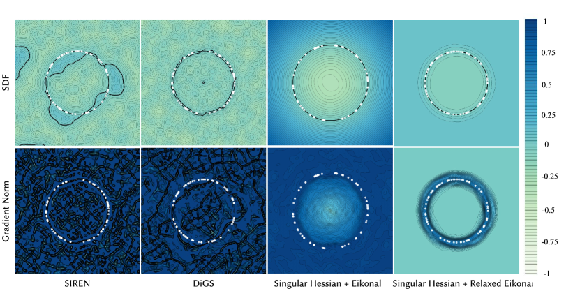
Given that the neural implicit function ${f}:\mathbb{R}^{3}\mapsto\mathbb{R}$ is utilized to approximate the SDF and our primary interest lies in the zero level set of $f$, our focus is on learning $f$ in the vicinity of the surface where the function value is close to 0, rather than approximating the SDF everywhere. This is illustrated in Fig. 4. The real SDF may not be differentiable for a smooth surface at all points. However, there must exist a narrow thin-shell space surrounding the surface within which the SDF is differentiable. This differentiable region is denoted by $\Omega$. Consider a point $x\in\Omega$ whose projection onto the surface is $x^{\prime}$. The Hessian matrix of the SDF at $x$, $\mathbf{H}_{\text{SDF}}(x)$, has a zero eigenvalue, with the gradient at $x$, $\boldsymbol{g}_{\text{SDF}}(x)$, being the corresponding eigenvector. Additionally, the direction aligns with the normal vector at $x^{\prime}$. As a result, we have $\mathbf{H}_{\text{SDF}}(x)\boldsymbol{g}_{\text{SDF}}(x)=\boldsymbol{0}$ and $\text{Det}(\mathbf{H}_{\text{SDF}}(x))=0$, which holds for any point in the differentiable region $\Omega$, see Fig. 3. This property can be easily derived with the Eikonal condition by differentiating both sides of the Eikonal equation $\lVert\nabla f\rVert=1$, refer to the reader (Mayost, 2014). This observation has led us to regularize the neural implicit function by enforcing a singular Hessian.

Suppose that $f$ is $C^{2}$ smooth, its Hessian $\mathbf{H}_{f}(x)$ is defined as the Jacobian of the gradient of $f$:

(8) $$\mathbf{H}_{f}(x)=\left[\begin{array}[]{lll}f_{xx}(x)&f_{xy}(x)&f_{xz}({x})\\ f_{yx}({x})&f_{yy}({x})&f_{yz}({x})\\ f_{zx}({x})&f_{zy}({x})&f_{zz}({x})\end{array}\right].$$

In general, it is desirable for $f$ to approach the real SDF as accurately as possible, at least in $\Omega$. Therefore, it is necessary to enforce $\mathbf{H}_{f}(x)\boldsymbol{g}_{\text{SDF}}(x)=\boldsymbol{0}$ or $\text{Det}(\mathbf{H}_{f}(x))=0$ for any point in $\Omega$. We utilize $\text{Det}(\mathbf{H}_{f}(x))=0$ for points in close proximity to the surface, since (1) the ground-truth gradient $\boldsymbol{g}_{\text{SDF}}(x)$ is unknown and (2) $\mathbf{H}_{f}(x)\boldsymbol{g}_{\text{SDF}}(x)=\boldsymbol{0}$ implies $\text{Det}(\mathbf{H}_{f}(x))=0$ but not vice versa. In implementation, we use $\mathcal{Q}_{\text{near}}$ to denote the query point set near the surface (sampling details will be given in Section 5). The singular-Hessian loss is formulated as follows:

(9) $$L_{\text{singularH}}=\int_{\mathcal{Q}_{\text{near}}}\lVert\text{Det}(\mathbf{H}_{f}(x))\lVert_{1}dx.$$

Figure 6. Unexpected critical points (red points) near the surface, result in undesired surface variations (left). To address this, we utilize the singular-Hessian term to suppress these variations and eliminate ghost geometry (right).

4.2. How singular Hessian works

Algebraic viewpoint.

According to the Taylor expansion,

(10) $$f(x)=f(x_{0})+\boldsymbol{g}_{f}^{\text{T}}(x-x_{0})+\frac{1}{2}(x-x_{0})^{\text{T}}\mathbf{H}_{f}(x)(x-x_{0}),$$

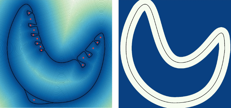
the utilization of $\text{Det}(\mathbf{H}_{f}(x))=0$ permits variation in the second-order term $\frac{1}{2}(x-x_{0})^{\text{T}}\mathbf{H}_{f}(x)(x-x_{0})$, but with fewer degrees of freedom. It is important to note that the Hessian energy is defined as $\|\mathbf{H}_{f}(x)\|_{2}^{2}$. When the Hessian energy is reduced to 0, all entries of $\mathbf{H}$ become 0, causing $f$ to become a linear field and diminishing its ability to accurately represent geometric details. In contrast to the Hessian energy, our singular Hessian term still allows $f$ to be sufficiently expressive even if the term is reduced to 0. See Fig. 5 for an illustration.

Morse theory.

The points in $\Omega$ (a thin-shell space surrounding the underlying surface) can be classified as either regular or critical, based on whether the gradient of function $f$ vanishes. The critical points can be further divided into (1) minimum points ($\mathbf{H}_{f}(x)$ does not have negative eigenvalues), (2) 1-saddle points (one negative eigenvalue), (3) 2-saddle points (two negative eigenvalues), and (4) maximum points (three negative eigenvalues). Let the numbers be respectively $c_{\text{min}},c_{\text{1-saddle}}$, $c_{\text{2-saddle}}$, and $c_{\text{max}}$. By taking $f$ as a Morse function defined in $\Omega$, the Euler characteristic of $\Omega$ is given by

(11) $$\chi(\Omega)=c_{\text{min}}-c_{\text{1-saddle}}+c_{\text{2-saddle}}-c_{\text{max}}.$$

Unnecessary surface variations are generally caused by an overly complicated function $f$ containing redundant critical points in $\Omega$, see Fig. 6. The enforcement of $\text{Det}(\mathbf{H}_{f}(x))=0$ drives $f$ toward simplicity by removing critical points in $\Omega$, but has no side effects for regular points satisfying $\text{Det}(\mathbf{H}_{f}(x))=0$. In other words, $\text{Det}(\mathbf{H}_{f}(x))=0$ helps eliminate a minimum point and a 1-saddle point, or a maximum point and a 2-saddle point, or a minimum point and a maximum point, or a 1-saddle point and a 2-saddle point, until the minimum number of critical points exist and precisely conforms to the Euler characteristic of $\Omega$. In contrast, the enforcement of the Hessian energy has side effects on regular points and results in a linear field whose Euler characteristic may be independent of $\Omega$. Therefore, $\text{Det}(\mathbf{H}_{f}(x))=0$ is a more relaxed constraint that still preserves the topology of $\Omega$.

Table 1. Quantitative comparison on Surface Reconstruction Benchmark (Williams et al., 2019). Note that the methods marked with ‘*’ require point normals. In each column, the best scores are highlighted in bold with underline, while the second best scores are highlighted with bold.

	Chamfer $\downarrow$		F-Score $\uparrow$
	mean	std.	mean	std.
SPSR∗ (Kazhdan et al., 2013)	4.36	1.56	75.87	18.57
DGP∗ (Williams et al., 2019)	4.87	1.64	73.34	18.56
SIREN (Sitzmann et al., 2020)	18.24	17.09	38.74	31.26
SAP (Peng et al., 2021)	6.19	1.75	57.21	11.66
iPSR (Hou et al., 2022)	4.54	1.78	75.07	19.18
PCP (Baorui et al., 2022b)	6.53	1.75	47.97	14.50
CAP-UDF (Zhou et al., 2022)	4.54	1.82	74.75	18.84
DiGS (Ben-Shabat et al., 2022)	4.16	1.44	76.69	18.15
Ours	3.76	0.98	81.38	13.73

Figure 7. We select two point clouds from Surface Reconstruction Benchmark (Williams et al., 2019) and give a visual comparison among SPSR (Kazhdan et al., 2013), CAP-UDF (Zhou et al., 2022), DiGS (Ben-Shabat et al., 2022) and ours. ‘*’ means that the approach requires normals. It can be seen from the highlighted differences that our algorithm can produce a surface with high fidelity.

Figure 8. Visual comparison of surface reconstruction under ShapeNet (Chang et al., 2015). The methods marked with ‘^∗’ require normals, and the methods marked with ‘⁺’ are supervision-based. Our method can faithfully recover the thin plates/tubes even if the input point cloud is only with 1K points.

4.3. Relaxing Eikonal Term

The Eikonal equation, denoted as $\|\nabla{f}\|_{2}=1$, is commonly used to characterize the first-order property of the SDF. Several research works have mimicked this condition by requiring $\|\nabla{f}\|_{2}=1$. However, for the surface reconstruction problem, the focus is solely on the zero-level set of $f$. It is sufficient to require that the gradient of $f$ does not vanish near the surface. Therefore, we relax the Eikonal constraint of $\|\nabla{f}\|=1$ into $\|\nabla{f}\|>\sigma_{\min}$:

(12) $$L_{\text{Eikonal}}^{\text{relax}}=\int_{\mathcal{P}}\text{ReLU}\left(-(\|\nabla f(x)\|-\sigma_{\min})\right)dx,$$

where ReLU is the operator of $\max(0,\cdot)$ and $\sigma_{\min}$ represents the minimum gradient norm that must be retained by the field. We set $\sigma_{\min}=0.8$ by default. Additionally, the condition is enforced exclusively for points belonging to the input point cloud.

Remark: Although $f$ is intended to approach the real SDF, they cannot be exactly identical. Relaxing the Eikonal constraint accommodates a wider range of possible candidates, allowing for the identification of the most desirable solution. In summary, by relaxing this condition, other terms can play a more significant role, providing $f$ with sufficient expressiveness.

4.4. Total loss

To this end, our total loss is formulated below:

(13) $$\begin{split}L_{\text{ours}}=&\lambda_{\text{manifold}}L_{\text{manifold}}+\lambda_{\text{non-manifold}}L_{\text{non-manifold}}+\\ &\lambda_{\text{Eikonal}}^{\text{relax}}L_{\text{Eikonal}}^{\text{relax}}+\lambda_{\text{singularH}}\tau L_{\text{singularH}}.\end{split}$$

where the parameter $\tau$ is an annealing factor, allowing for a coarse-to-fine learning process that learns geometric details gradually. The annealing factor $\tau$ remains 1 during the first 20% iterations, then linearly decreases to 0.0003 during the 20% to 40% iterations, and finally decreases to 0.00003 at the termination. We tune weights to our preferred setting ($\lambda_{\text{manifold}}$= $7000$, $\lambda_{\text{non-manifold}}$ = $600$, $\lambda_{\text{Eikonal}}^{\text{relax}}$ = $50$) and use consistent hyperparameters over the different datasets.

Table 2. Quantitative comparison on ShapeNet (Chang et al., 2015). Note that the methods marked with ‘*’ require point normals, and the methods marked with ‘⁺’ are supervision based. In each column, the best scores are highlighted in bold, while the second best scores are highlighted in bold with underlining.

	1K points						3K points
	Normal C. $\uparrow$		Chamfer $\downarrow$		F-Score $\uparrow$		Normal C. $\uparrow$		Chamfer $\downarrow$		F-Score $\uparrow$
	mean	std.	mean	std.	mean	std.	mean	std.	mean	std.	mean	std
SPSR∗ (Kazhdan et al., 2013)	91.89	4.76	9.35	7.66	46.91	26.06	95.50	3.30	4.66	4.64	75.28	25.76
NSP∗ (Williams et al., 2021)	87.05	6.05	12.51	7.29	36.17	21.56	90.74	5.48	8.85	6.96	52.42	28.55
SAL (Atzmon and Lipman, 2020)	82.99	11.11	47.46	50.57	18.16	19.15	86.69	9.66	29.98	31.86	25.76	22.43
IGR (Gropp et al., 2020)	79.26	12.27	77.68	59.55	22.48	32.08	80.85	11.88	62.54	48.44	26.28	35.91
SIREN (Sitzmann et al., 2020)	79.91	8.87	38.04	46.02	25.02	23.52	83.79	10.20	34.19	46.77	32.34	30.13
DiGS (Ben-Shabat et al., 2022)	92.67	6.03	7.01	5.52	58.72	29.77	95.82	4.44	4.59	4.94	78.87	27.34
OSP (Baorui et al., 2022a)	91.89	5.52	8.77	6.76	47.57	23.45	94.73	3.94	6.80	6.61	59.12	25.82
iPSR (Hou et al., 2022)	87.88	7.26	13.16	11.78	39.36	25.11	93.22	5.26	5.95	5.97	68.42	26.36
PGR (Lin et al., 2022)	89.53	5.35	10.49	6.52	37.61	19.14	91.90	4.93	7.34	4.81	51.44	23.12
SAP+ (Peng et al., 2021)	94.92	3.60	4.64	3.71	73.50	25.02	96.33	3.24	3.75	4.16	84.79	20.94
POCO+ (Boulch and Marlet, 2022)	94.79	4.15	4.53	4.05	75.56	26.46	96.41	3.53	3.62	4.21	85.42	23.13
Ours	95.10	4.04	4.26	3.11	80.51	21.48	97.05	2.91	3.08	2.64	90.71	16.28

Figure 9. Visual comparison of surface reconstruction under ABC (Koch et al., 2019). Our method can effectively recover the CAD features (e.g., small holes and thin plates).

5. EXPERIMENTS

In this section, the details regarding parameter selection are first presented, followed by an explanation of the metrics and evaluation protocol, more details can be checked in our supplementary material. The proposed approach is then evaluated on various datasets, including both synthetic and real scans. Additionally, the approach is tested in shape space learning for human body scans.

5.1. Implementation Details

Experiments were conducted using an NVIDIA GeForce RTX 3090 graphics card with 24GiB video memory and an AMD EPYC 7642. A SIREN-based MLP with its initialization method was used for the network (Sitzmann et al., 2020). Inputs were first normalized to the range $\left[-1,1\right]^{3}$ for SIREN-based MLP. $\mathcal{Q}_{\text{far}}$ is uniformly sampled within the bounding box of the input point cloud $\mathcal{P}$, while $\mathcal{Q}_{\text{near}}$ is sampled following (Gropp et al., 2020; Baorui et al., 2021; Zhou et al., 2022) based on Gaussians distribution centered on each input point. For a point in $p\in\mathcal{P}$, the Gaussian function is centered at $p_{i}$ with the mean and standard deviation set to the distance to its $k$-th ($k=50$ by default). We sample one point for each distribution. The number of points in both $\mathcal{Q}_{\text{near}}$ and $\mathcal{Q}_{\text{far}}$ complies with the batch size (15K by default).

5.2. Metrics

Comparison indicators include normal consistency, chamfer distances, and F-Score. Normal consistency (expressed as a percentage and abbreviated as ‘Normal C.’) reflects the degree of agreement between the normals of the reconstructed surface and those of the ground-truth surface. Chamfer distance (scaled by $10^{3}$ and using $L_{1}$-norm) measures the fitting tightness between the two surfaces, and F-Score (expressed as a percentage) indicates the harmonic mean of precision and recall (completeness). The default threshold for F-Score is set to 0.005. All meshes are uniformly scaled to $\left[-0.5,0.5\right]^{3}$, with 100K points sampled from each mesh for evaluation.

Table 3. Quantitative comparison on ABC (Koch et al., 2019) and Thingi10K (Zhou and Jacobson, 2016). Each raw point cloud has 10K points. The methods marked with ‘*’ require point normals, and the methods marked with ‘⁺’ are supervision-based. In each column, the best scores are highlighted in bold, while the second best scores are highlighted in bold with underlining.

	ABC						Thingi10K
	Normal C. $\uparrow$		Chamfer $\downarrow$		F-Score $\uparrow$		Normal C. $\uparrow$		Chamfer $\downarrow$		F-Score $\uparrow$
	mean	std.	mean	std.	mean	std.	mean	std.	mean	std.	mean	std
SPSR∗ (Kazhdan et al., 2013)	95.16	4.48	4.39	3.05	74.54	26.65	97.15	2.95	3.93	1.79	77.03	23.71
SAL (Atzmon and Lipman, 2020)	86.25	8.39	17.30	14.82	29.60	18.04	92.85	5.01	13.46	7.97	27.56	14.64
IGR (Gropp et al., 2020)	82.14	16.12	36.51	40.68	43.47	40.06	90.20	10.61	27.80	34.8	54.28	39.99
SIREN (Sitzmann et al., 2020)	82.26	9.24	17.56	15.25	30.95	22.23	88.30	6.53	17.69	13.47	26.20	19.74
Neural-Pull (Baorui et al., 2021)	94.23	4.57	6.73	5.15	42.67	10.75	96.15	2.80	5.89	1.12	46.44	8.53
SAP (Peng et al., 2021)	81.59	10.61	15.18	16.60	45.88	33.67	92.60	7.03	10.61	13.84	53.32	31.91
DiGS (Ben-Shabat et al., 2022)	94.48	6.12	6.91	6.94	66.22	32.01	97.25	3.30	5.36	5.59	74.45	27.11
iPSR (Hou et al., 2022)	93.15	7.47	4.84	4.06	71.59	24.96	96.46	3.57	4.41	2.94	74.88	22.72
PGR (Lin et al., 2022)	94.11	4.63	4.52	2.13	68.91	27.86	96.80	3.25	4.22	2.01	72.86	22.98
POCO+ (Boulch and Marlet, 2022)	92.90	7.00	6.05	6.80	68.29	26.05	95.16	5.00	5.61	9.42	73.92	25.79
NG+ (Huang et al., 2022a)	95.88	3.88	3.60	1.38	81.38	20.39	97.71	2.68	3.16	1.07	86.29	17.39
Ours	97.42	2.37	3.27	1.78	88.62	13.87	98.23	1.98	3.00	2.62	93.50	11.84

Figure 10. Visual comparison of surface reconstruction under Thingi10K (Zhou and Jacobson, 2016). Our method can recover high-fidelity geometric details.

5.3. Overfitting Surface Reconstruction

A SIREN network consisting of 4 hidden layers with 256 units was used to conduct experiments. The discrete mesh of the zero-level set of the implicit function was extracted using the marching cubes algorithm (Lewiner et al., 2003) from scikit-image (van der Walt et al., 2014) with $256^{3}$ grids. For overfitting experiments, the Adam optimizer (Kingma and Ba, 2014) was used with a learning rate of $5\times 10^{-5}$ and a total of 10K iterations by default.

5.3.1. Surface Reconstruction Benchmark (SRB)

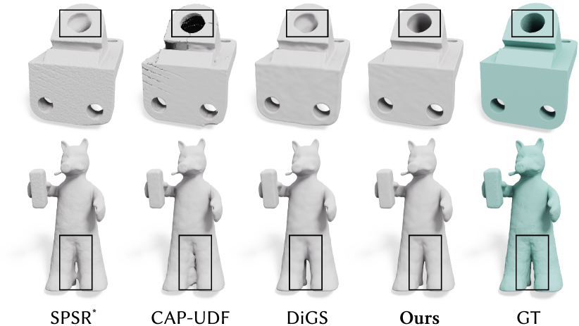
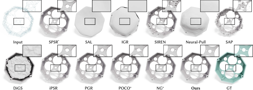
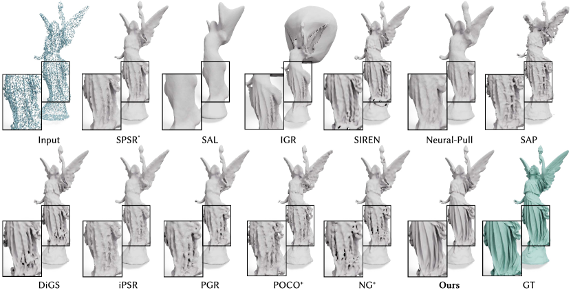
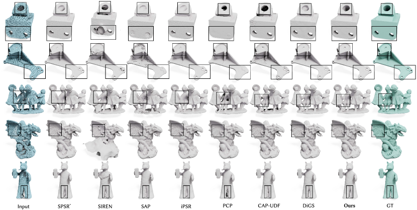
The Surface Reconstruction Benchmark (SRB) (Williams et al., 2019) comprises five shapes, each with challenging features such as missing parts and rich details. Approaches for comparison include screened Poisson surface reconstruction (SPSR) (Kazhdan et al., 2013), SIREN (Sitzmann et al., 2020), DGP (Williams et al., 2019), Shape as points (SAP) (Peng et al., 2021), iPSR (Hou et al., 2022), Predictive Context Priors (PCP) (Baorui et al., 2022b), CAP-UDF (Zhou et al., 2022) and DiGS (Ben-Shabat et al., 2022). It should be noted that SPSR and DGP leverages normals provided by the input scans. As demonstrated in Tab. 1 and Fig. 7, our method outperforms existing methods in terms of both Chamfer distance and F-score. In particular, the visual comparison in Fig. 7 shows that our method can recover the hole feature of the Anchor model despite the lack of points on the inner wall and preserve the nearby gaps of the Lord Quas model.

Figure 11. Visual comparison of real raw scans from (Huang et al., 2022b) and Aim@Shape Shape Repository. Our method can deal with real scans and recover the details.

5.3.2. ShapeNet

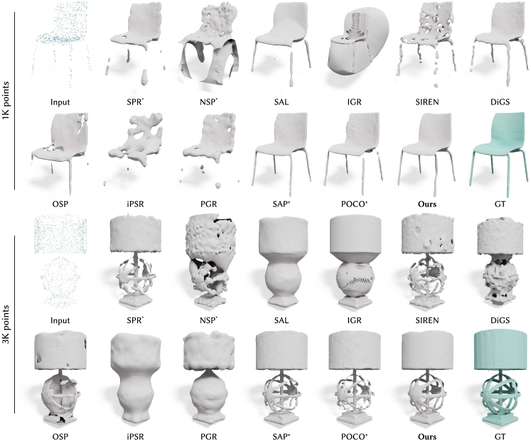
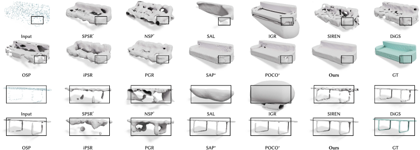
The ShapeNet (Chang et al., 2015) comprises a diverse range of CAD models. We follow the splitting of (Williams et al., 2021) for the 13 categories of shapes with totally 260 shapes. We perform the comparison under two settings, i.e., “1K points” and “3K points”. Baseline approaches include the screened Poisson surface reconstruction (SPSR) (Kazhdan et al., 2013), NSP (Williams et al., 2021), SAL (Atzmon and Lipman, 2020), IGR (Gropp et al., 2020), SIREN (Sitzmann et al., 2020), DiGS (Ben-Shabat et al., 2022), OnSurfacePrior (OSP) (Baorui et al., 2022a), iPSR (Hou et al., 2022) and PGR (Lin et al., 2022). It should be noted that SPSR and NSP need to input normals. To make the comparison more convincing, we provide ground-truth normals to those methods that require normals. Additionally, learnable baselines such as Points (SAP) (Peng et al., 2021) and POCO (Boulch and Marlet, 2022) are included for comparison and re-trained from scratch on the ShapeNet dataset with 1K points and 3K points settings, respectively. Based on the quantitative comparison in Tab. 2 and the visual comparison in Fig. 8, it is evident that the majority of existing methods are unable to effectively handle data sparsity. This issue is particularly pronounced when thin-walled plates and tubes are present, as it significantly increases the difficulty of reconstruction. In contrast, our method is able to effectively suppress unnecessary variations near the surface and adapt the implicit representation to the inherent complexity encoded by the point cloud. Furthermore, our reconstruction accuracy surpasses even that of supervision-based methods SAP and POCO.

5.3.3. ABC and Thingi10K

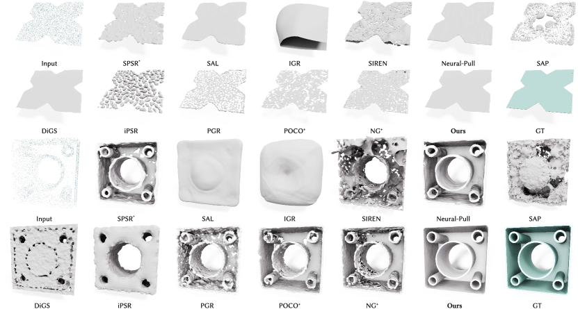
The ABC dataset (Koch et al., 2019) comprises a diverse collection of CAD meshes, while the Thingi10K dataset (Zhou and Jacobson, 2016) contains a variety of shapes with intricate geometric details. We follow (Erler et al., 2020) to perform splitting that 100 shapes for each dataset and randomly sample 10K points from each mesh. The baseline approaches include the screened Poisson surface reconstruction (SPSR) (Kazhdan et al., 2013), SAL (Atzmon and Lipman, 2020), IGR (Gropp et al., 2020), SIREN (Sitzmann et al., 2020), Neural-Pull (Baorui et al., 2021), SAP (Peng et al., 2021), DiGS (Ben-Shabat et al., 2022), iPSR (Hou et al., 2022) and PGR (Lin et al., 2022). It is important to note that we find the supervision version of SAP does not generalize well on the shape not present on the trainset (ShapeNet) when using the global PointNet-based encoder. As such, we compare against the unsupervised version of SAP. Additionally, We include supervision methods POCO (Boulch and Marlet, 2022) and Neural Galerkin (NG, the version without normals) (Huang et al., 2022a) for comparison. In order to assess the generalization capabilities of the supervised methods, we retrained them using a setting of 10K points on the ShapeNet dataset. The quantitative comparison statistics are recorded in Tab. 3. Furthermore, visual comparisons conducted using the ABC dataset (Koch et al., 2019) (as shown in Fig. 9) demonstrate that our method is capable of effectively recovering CAD features such as small holes and thin plates. Similarly, visual comparisons conducted using the Thingi10K dataset (Zhou and Jacobson, 2016) (as shown in Fig. 10) demonstrate that our method is capable of recovering high-fidelity geometric details.

5.3.4. Real Scans

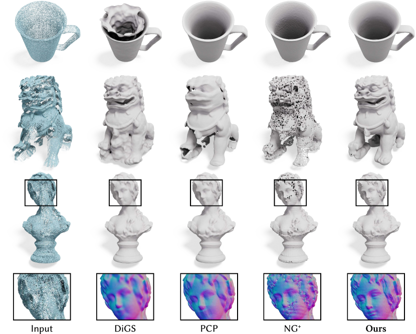
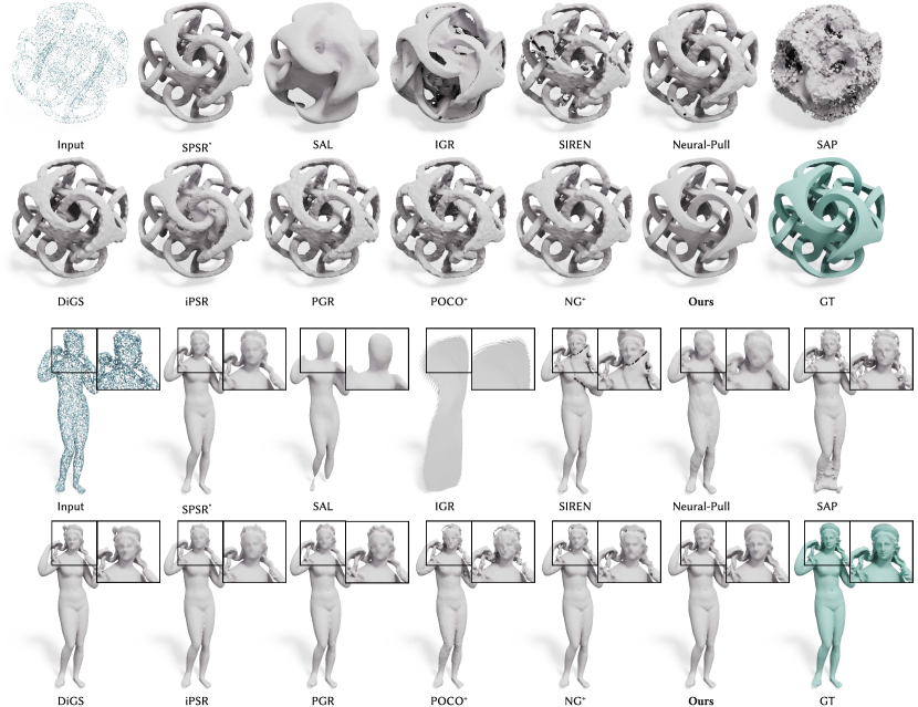
We also evaluated our method on real scans with various artifacts from (Huang et al., 2022b) and AIM@SHAPE-VISIONAIR. The point clouds from (Huang et al., 2022b) were scanned using a SHINING 3D Einscan SE scanner and exhibit noise and non-uniform densities. The point clouds from AIM@SHAPE-VISIONAIR were scanned using a Kreon scanner and exhibit highly non-uniform line distributions and unnatural scanner noise. We included DiGS (Ben-Shabat et al., 2022), PCP (Baorui et al., 2022b), and supervised method Neural Galerkin (NG, without normals) (Huang et al., 2022a) as baselines for comparison. Qualitative results can be seen in Fig. 11. Our method effectively recovers the details and concave parts of the shapes, while other methods do not. In particular, the supervised method Neural Galerkin performs poorly when applied to real scans that have point distributions not present in its training dataset (as shown in the second row of Fig. 11).

5.3.5. Large Scans

We evaluated the ability of our method to handle large-sized point clouds using three shapes from the ThreedScans dataset (Laric, 2012), randomly sampling approximately 300K points from each shape. For comparison, we include SIREN (Sitzmann et al., 2020) with ground truth oriented normals, PCP (Baorui et al., 2022b), DiGS (Ben-Shabat et al., 2022), and the learnable method of Neural Galerkin (NG, without normals) (Huang et al., 2022a). For this experiment, the final mesh is extracted at a resolution of $512^{3}$ rather than $256^{3}$. Additionally, we sampled 1M points to analyze the distance between two surfaces and set the F-Score threshold to 0.001 (denoted as F-Score^△). Quantitative comparison statistics are provided in Tab. 4, while visual comparisons can be seen in Fig. 12. It is important to note that we trimmed surplus parts from SIREN’s results. PCP and DiGS tend to produce smooth results without geometric details, with DiGS’ smoothing energy weakening geometric details. Neural Galerkin is a supervised method and thus exhibits weaker generalization capabilities. In summary, for large-sized point clouds, our method outperforms existing unoriented approaches and is even superior to the “with normals” version of SIREN.

Figure 12. Tests on large scans (about 30K points) from  ThreedScans (Laric, 2012) (CC BY-NC-SA). We include SIREN (Sitzmann et al., 2020) (with ground-truth normals), DiGS (Ben-Shabat et al., 2022), PCP (Baorui et al., 2022b) and NG (Huang et al., 2022a) (supervision-based) for comparison. In contrast to the SOTA methods, our approach can recover high-fidelity geometry details from unoriented point clouds, and our results are comparable to SIREN trained with ground-truth normals.

Figure 13. Visual comparison of shape space learning under DFAUST (Bogo et al., 2017). Our method can learn shape space without normals or additional supervision. By a fine-turning operation at the inference stage, our method can produce faithful shapes with great details.

Table 4. Quantitative comparison on large scans (Laric, 2012). The methods marked with ‘^∗’ require normals, and the methods marked with ‘⁺’ are supervision based.

	Normal C. $\uparrow$		Chamfer $\downarrow$		F-Score${}^{\vartriangle}~{}\uparrow$
	mean	std.	mean	std.	mean	std.
SIREN∗ (trimmed) (Sitzmann et al., 2020)	98.38	0.30	0.96	0.17	63.61	19.62
PCP (Baorui et al., 2022b)	94.32	2.58	4.44	1.41	11.83	9.41
DiGS (Ben-Shabat et al., 2022)	97.41	0.62	0.92	0.22	63.78	21.91
NG+ (Huang et al., 2022a)	85.97	9.10	3.02	2.09	31.01	20.67
Ours	98.44	0.15	0.74	0.09	79.77	9.90

5.4. Learning Shape Space

Dataset

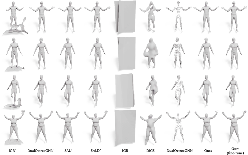
The D-Faust dataset (Bogo et al., 2017) contains high-resolution raw scans (triangle soups) of 10 humans in various poses. We followed the methodology outlined in DualOctreeGNN (Wang et al., 2022) to perform splitting, using 6K scans for training and 2K scans for testing. The raw point clouds used as input are incomplete and noisy due to occlusion during the scanning process and the limited precision of scanners.

Training details

During the training phase, we utilized an encoder based on Convolutional Occupancy Networks (Songyou et al., 2020) to encode shapes that enable shape space learning. Specifically, we projected sparse on-surface point features obtained using a modified PointNet (Qi et al., 2017) onto a regular 3D grid and used a convolutional module to propagate these features to the off-surface area. The query feature was then obtained using trilinear interpolation. Additionally, we employed FiLM conditioning (Chan et al., 2021), which applies an affine transformation to the network’s intermediate features, as SIREN struggles with handling high-dimensional inputs (Chan et al., 2021; Mehta et al., 2021). Furthermore, inspired by (Tang et al., 2021b), we fine-tuned the network during the inference phase to perform accurate geometry learning for high-fidelity surface reconstruction using our novel loss. Our models were trained for 200 epochs using the AMSGrad optimizer (Reddi et al., 2018) with an initial learning rate of $10^{-4}$, which was decayed to $10^{-6}$ using cosine annealing (Loshchilov and Hutter, 2017). The training set was divided into mini-batches containing 32 different shapes (with accumulated gradients), with each shape being randomly sampled as 10K points.

Table 5. Quantitative comparison on DFAUST (Bogo et al., 2017). The methods marked with ‘^∗’ require normals, and the methods marked with ‘⁺’ are supervision based. In each column, the best scores are highlighted in bold, while the second best scores are highlighted in bold with underlining.

	Normal C. $\uparrow$		Chamfer $\downarrow$		F-Score $\uparrow$
	mean	std.	mean	std.	mean	std.
IGR∗ (2020)	92.02	3.34	29.01	33.61	73.32	14.05
DualOctreeGNN∗ (2022)	97.65	0.34	1.78	3.70	97.48	1.03
SAL+ (2020)	96.77	0.81	2.82	4.67	91.35	9.15
SALD∗+ (2021)	97.04	0.92	3.06	1.32	88.56	12.73
IGR (2020)	57.93	3.40	48.56	2.35	6.54	0.11
DiGS (2022)	87.60	1.91	11.87	4.56	37.77	7.11
DualOctreeGNN (2022)	92.42	0.45	3.02	2.38	85.77	3.50
Ours	96.22	0.55	2.50	0.51	94.45	1.48
Ours (fine-tune)	97.05	0.50	1.96	0.27	96.46	0.93

Results

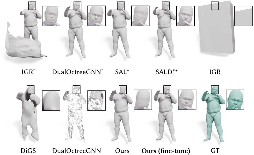
The baseline approaches we compared against include IGR (Gropp et al., 2020), SAL (Atzmon and Lipman, 2020), SALD (Atzmon and Lipman, 2021), DualOctreeGNN (Wang et al., 2022), and DiGS (Ben-Shabat et al., 2022). We also demonstrated the results of IGR and DualOctreeGNN trained without normals. As shown in Fig. 13 and Tab. 5, while IGR is capable of generating detailed results, it also produces spurious planes away from the input. SAL, which is supervised using unsigned distance, can only produce smooth results. SALD, with the support of normal supervision, can generate more detailed results but its reconstruction accuracy is worse than that of SAL due to a large systematic misalignment that does not respect input poses. In contrast, DualOctreeGNN produces the most impressive results due to its well-designed octree network’s ability to capture local priors for details. However, the performance of both IGR and DualOctreeGNN is compromised without normals. In particular, the resulting surfaces of DualOctreeGNN for point clouds without input normals are not watertight, despite the small Chamfer distances. While DiGS also being based on SIREN, it cannot produce reliable results. In summary, our method is capable of learning shape space without requiring input normals or additional supervision and still produces faithful shapes. It is important to note that we did not fine-tune other auto-encoder-based methods (except for IGR and DiGS, which leverage auto-decoder and have to be optimized during the inference stage) as our method consistently outperformed unoriented input even without fine-tuning.

Table 6. Comparison about different gradient constraints.

	Normal C. $\uparrow$		Chamfer $\downarrow$		F-Score $\uparrow$
	mean	std.	mean	std.	mean	std.
$\text{Eikonal}_{\text{all}}$	97.33	2.75	3.74	2.86	88.04	15.36
$\text{Eikonal}_{\text{half}}$	97.52	2.98	3.42	2.80	89.07	15.22
$\sigma_{\text{min}}={0.6}$	97.55	2.84	3.34	2.47	89.92	14.58
$\sigma_{\text{min}}={0.8}$ (Ours)	97.82	2.18	3.13	2.20	91.06	12.85
$\sigma_{\text{min}}={1.0}$	97.48	3.18	3.35	2.57	89.42	14.70

5.5. Ablation Studies

We conducted ablation studies using two datasets: ABC (Koch et al., 2019) and Thingi10K (Zhou and Jacobson, 2016). Each dataset comprised 100 shapes, discretized into 10K points. To examine the effects of hyper-parameters, we also utilized the SRB (Williams et al., 2019) dataset and five shapes from the Stanford 3D Scanning Repository: Armadillo, Bunny, Dragon, Asian Dragon, and Thai Statue. More ablation studies can be found in our supplementary material.

Table 7. Comparison about different smooth energy forms: Dirichlet Energy ($E_{D}$), Hessian Energy ($E_{H_{2}}$), and Hessian Energy based-$L_{1}$ ($E_{H_{1}}$).

	Normal C. $\uparrow$		Chamfer $\downarrow$		F-Score $\uparrow$
	mean	std.	mean	std.	mean	std.
$E_{D}$	94.42	3.71	8.13	6.75	64.45	31.23
$E_{H_{2}}$	97.62	2.58	3.33	2.28	87.94	17.70
$E_{H_{1}}$	97.45	2.74	3.85	3.90	87.92	18.48
Ours	97.82	2.18	3.13	2.20	91.06	12.85

Figure 14. Visual comparison of different smooth energy forms. Our method is superior to the other approaches in terms of the ability to recover geometry details.

5.5.1. Relaxing Eikonal Constraint

In the following, we will demonstrate the effectiveness of relaxing the Eikonal constraint. Our relaxation technique is two-fold. First, we hope that the gradients do not vanish, rather than be exactly a unit vector. Second, the gradient constraint is specified around the surface rather than in the whole space. For the ablation study purpose, we test the effect of substituting the traditional Eikonal condition for our relaxed gradient constraint. The first setting named $\text{Eikonal}_{\text{all}}$, requires the gradients at all points, i.e., the input points and the query points, to be unit vectors. The second setting, named $\text{Eikonal}_{\text{half}}$, is to specify the Eikonal constraint at the input points. At the same time, we test different choices of $\sigma_{min}$ for our approach, i.e., $0.6,0.8,\text{and}\ 1$. The statistics in Tab. 6 show that (1) it seems better to specify the Eikonal constraint at the input points than at all the points, and (2) the inequality of $\|\nabla f\|_{2}\geq\sigma_{min}$ is easier to solve compared with $\|\nabla f\|_{2}=1$.

5.5.2. Comparison to Smooth Energy Forms

The commonly used Dirichlet energy is as follows:

(14) $$E_{D}=\frac{1}{2}\int_{\mathcal{P}\cup\mathcal{Q}_{\text{far}}}\|\nabla f(x)\|_{2}^{2}dx,$$

where $\Omega$ is the space of the whole bounding box. The commonly used Hessian energy is as follows:

(15) $$E_{H_{2}}=\int_{\mathcal{P}\cup\mathcal{Q}_{\text{far}}}\|\mathbf{H}_{f}(x)\|_{2}^{2}dx.$$

Zhang et al. (2022) leveraged $L_{1}$-based Hessian:

(16) $$E_{H_{1}}=\int_{\mathcal{P}\cup\mathcal{Q}_{\text{far}}}\|\mathbf{H}_{f}(x)\|_{1}dx.$$

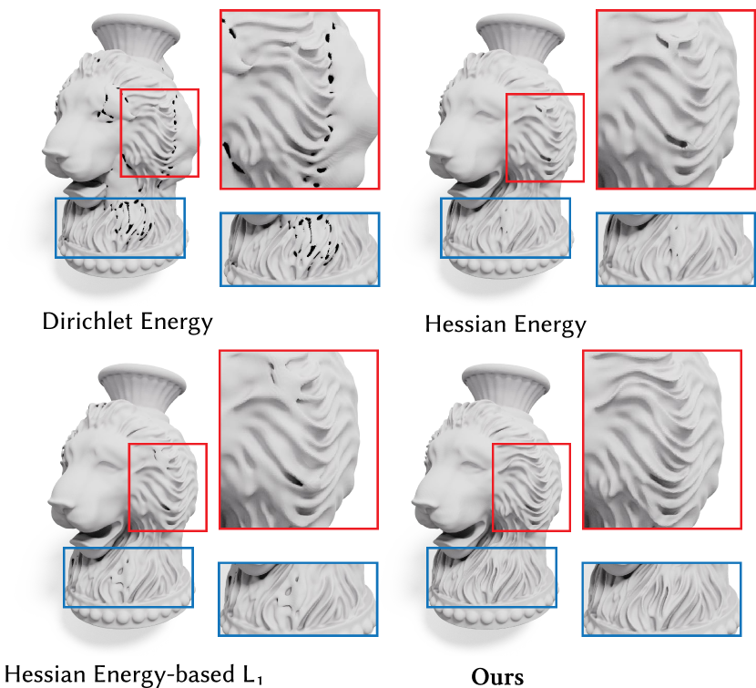
To ensure fairness in our evaluation, we combined the smoothness energy with relaxed Eikonal conditions (as described in Eq. 12) to demonstrate the effectiveness of $L_{\text{singularH}}$. As shown in Tab. 7 and Fig. 14, our method not only suppresses ghost geometry but also recovers high-fidelity geometric details. This demonstrates its superiority over both the Dirichlet energy, which produces ghost geometry, and the Hessian energy, which produces over-smoothed results possibly with adhesion in the area of sharp, thin features. It is important to note that when the Hessian energy becomes zero, all entries of $\mathbf{H}$ become zero, causing the SDF to degenerate into a linear function and diminishing its ability to accurately represent geometric details. In contrast, our term $L_{\text{singularH}}:\text{Det}(\mathbf{H}_{f})=0$ is more conservative, allowing for flexibility and capacity to recover geometric details. DiGS (Ben-Shabat et al., 2022) utilizes another smoothness energy form, Laplacian energy of the Hessian matrix, we compare against it in the next subsection.

Table 8. Quantitative comparison with DiGS (Ben-Shabat et al., 2022). Based on the comparison, our method exhibits a bigger advantage under different settings.

	Ours Weights	SIREN Init.	Eikonal Relax	Normal C. $\uparrow$		Chamfer $\downarrow$		F-Score $\uparrow$
				mean	std.	mean	std.	mean	std.
DiGS				95.86	4.71	6.13	6.26	70.34	29.56
			✓	96.15	4.94	5.08	4.65	75.10	27.96
		✓		95.59	5.06	5.89	7.03	76.02	30.48
		✓	✓	96.51	4.48	5.00	6.19	81.40	26.11
	✓	✓	✓	96.32	3.35	4.71	5.27	79.71	26.32
Ours	✓		✓	95.36	4.39	5.79	4.81	74.57	25.60
	✓	✓		97.33	2.75	3.74	2.86	88.04	15.36
		✓	✓	96.55	4.60	4.52	5.06	84.50	20.94
	✓	✓	✓	97.82	2.18	3.13	2.20	91.06	12.85

5.5.3. Comparison with DiGS

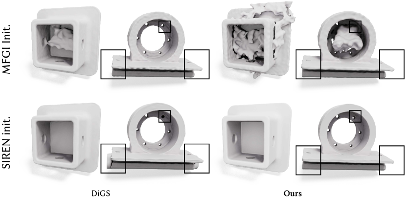
DiGS (Ben-Shabat et al., 2022) is another unoriented point cloud reconstruction method based on SIREN (Sitzmann et al., 2020). Notably, DiGS leverages the well-known smoothness of Laplacian energy based on the Hessian matrix for reconstruction. We conduct comprehensive experiments with DiGS and present the results in Tab. 8, which demonstrate that our method outperforms DiGS. Our observations are three-fold. First, we relax the Eikonal constraint in DiGS using our gradient constraint and found that DiGS produced better results with our proposed gradient constraint. Second, as shown in Fig. 15, the MFGI-based initialization, which initializes the SIREN network as an approximate sphere, is unable to reconstruct the concave parts of CAD shapes. In contrast, initializing SIREN directly appears to produce better results. However, unlike our approach, DiGS does not consistently yield better results when switching to direct SIREN initialization.

Finally, even when using the weighting scheme of DiGS $(\lambda_{\text{manifold}}$, $\lambda_{\text{non-manifold}},\lambda_{\text{Eikonal}})=(3000,100,50)$, our method still outperforms all variants of DiGS. If the weights are adjusted to our preferred setting ($\lambda_{\text{manifold}}$= $7000$, $\lambda_{\text{non-manifold}}$ = $600$, $\lambda_{\text{Eikonal}}^{\text{relax}}$ = $50$), our method exhibits an even greater advantage, while the performance of DiGS variants diminishes.

Figure 15. The ablation studies for initiation methods. DiGS (Ben-Shabat et al., 2022) is more sensitive to initiation. Both initiation methods cannot produce reliable results.

6. Conclusions

Learning the implicit neural representation from an unoriented point cloud is a fundamental task. In this paper, we propose to regularize the implicit function by enforcing singular Hessian near the surface. Extensive experimental results demonstrate that our approach exhibits the superior ability to recover high-fidelity geometric details in the presence of various imperfections.

Appendix A Additional Ablation Studies

Table 9. Ablation studies on the loss functions.

Eikonal Relax	Singular Hessian Term	Our weights	Normal C. $\uparrow$		Chamfer $\downarrow$		F-Score $\uparrow$
			mean	std.	mean	std.	mean	std.
			85.28	6.53	17.62	14.37	28.58	20.99
✓			88.54	6.71	15.55	11.33	36.64	31.15
	✓		96.34	3.44	4.25	5.06	84.38	20.08
		✓	93.74	4.85	9.45	8.35	61.68	32.83
✓	✓		96.55	4.60	4.52	4.17	84.50	20.94
✓		✓	94.85	3.54	6.53	3.99	70.92	25.21
	✓	✓	97.33	2.75	3.74	2.86	88.04	15.36
✓	✓	✓	97.82	2.18	3.13	2.20	91.06	12.85

Table 10. Comparison of the weights of $L_{\text{singularH}}$ and procedure of coarse-to-fine under SRB (Williams et al., 2019) dataset.

	Chamfer $\downarrow$		F-Score $\uparrow$
	mean	std.	mean	std.
$\lambda_{\text{singularH}}=0.3$ no-decay	4.29	1.38	75.36	15.99
$\lambda_{\text{singularH}}=3$ no-decay	5.02	1.83	70.76	15.12
$\lambda_{\text{singularH}}=30$ no-decay	7.41	2.78	56.90	11.56
$\lambda_{\text{singularH}}=0.3$ & decay	3.88	1.12	78.94	16.45
$\lambda_{\text{singularH}}=3$ & decay (Ours)	3.76	0.98	81.38	13.73
$\lambda_{\text{singularH}}=30$ & decay	4.01	1.37	77.14	14.07

A.1. Loss functions

We conduct experiments to observe the effects of the loss functions in Tab. 9. Compared with the original unoriented version of SIREN (Sitzmann et al., 2020), our method differs in three main ways: relaxed Eikonal constraint, singular Hessian term, and our preferred settings for loss weights. These three factors are mutually influenced and simply tuning the weights cannot improve the overall performance. Instead, enabling all three factors results in a significant improvement in performance. It is important to note that our method outperforms other fitting-based methods even with only $L_{\text{singularH}}$ (without $L_{\text{Eikonal}}^{\text{relax}}$) and our preferred weights settings.

\begin{overpic}[width=433.62pt]{figures/abl_weight.pdf} \par\put(17.0,28.0){(a)} \par\put(48.5,28.0){(b)} \par\put(82.0,28.0){(c)} \par\put(17.0,-3.0){(d)} \par\put(49.0,-3.0){(e)} \par\put(82.0,-3.0){(f)} \par\end{overpic}

Figure 16. Comparison about different $\lambda_{\text{singularH}}$ and coarse-to-fine training curriculum under SRB (Williams et al., 2019) that has different point clouds artifacts. From left to right: (a) $\lambda_{\text{singularH}}=0.3\&no-decay$, (b) $\lambda_{\text{singularH}}=3\&no-decay$ (c) $\lambda_{\text{singularH}}=30\&no-decay$, (d) $\lambda_{\text{singularH}}=0.3\&decay$, (e) $\lambda_{\text{singularH}}=3\&decay$, and $\lambda_{\text{singularH}}=30\&decay$ .

A.2. Weight of $L_{\text{singularH}}$ and Coarse-to-fine training curriculum

We investigate the effects of several design choices made for $L_{\text{singularH}}$ over SRB (Williams et al., 2019) dataset with noise or missing parts shapes in Tab. 10. First, we examine the influence of different $L_{\text{singularH}}$ settings without annealing. Fig. 16 shows that larger weights lead to over-smooth results with topological errors, while smaller weights cannot fill the missing parts. Additionally, all results exhibit some topology errors without annealing. We further test the effect of the annealing function $\tau$ with different $\lambda_{\text{singularH}}$ settings. Our method achieves the best performance with initialization $\lambda_{\text{singularH}}=3$, balancing geometric details and robustness to point cloud artifacts. The remaining question is what are the effects if we keep a very small weight all the time? In Fig. 17, we show the results with weight $0.01$ at different iterations. It can be seen our method can also work well with a constant small weight, but it may take a longer time to converge without the coarse-to-fine training curriculum.

Table 11. We compare the impact of the parameter $k$ on the sampling process of $Q_{near}$ using different numbers of points from the Stanford 3D Scanning Repository. The evaluation metric used in this comparison is the Chamfer distance.

	500	1000	10000	100000
$k=5$	9.10	5.88	2.54	2.44
$k=25$	9.40	5.64	2.51	2.14
$k=50$	8.86	5.84	2.61	2.10
$k=75$	9.31	5.88	2.46	2.17
$k=100$	9.41	5.56	2.55	2.14

Figure 17. The reconstruction result of at different iterations with small weight ($0.01$). It requires a longer time to converge.

A.3. The Effect of $Q_{near}$ range

Finally, we discuss the effect of the query location range. By default, we used the Gaussian destruction with the distance of $k=50$ neighbors as the standard deviation for sampling $Q_{near}$. Here, we use several candidates including $\{k=5,k=25,k=50,k=75,k=100\}$, to test the effects of different ranges of $Q_{near}$. We report the results under five shapes from Stanford 3D Scanning Repository with different point clouds resolutions $\{500,1000,10000,100000\}$ in Tab. 11. The comparison results indicate that there are no significant differences observed with different values of $k$. We choose to set $k=50$ for our study. The comparison shows that a query location range that is either too small or too large will degrade surface reconstruction performance.

A.4. Combined with Softplus

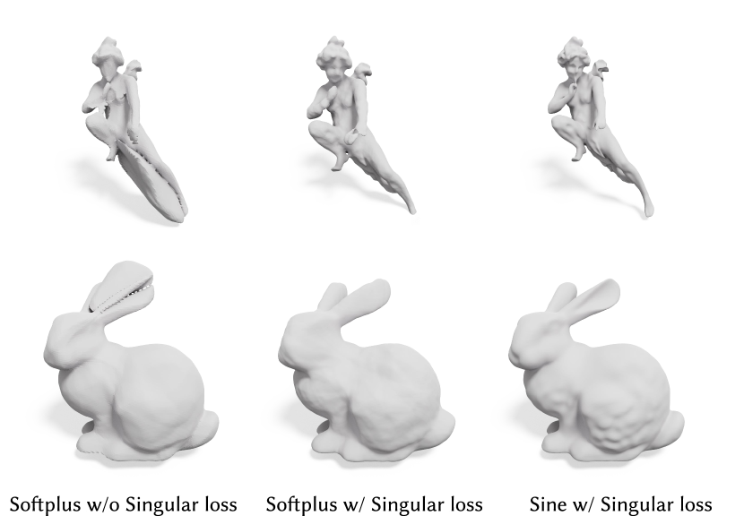
Our approach is general and can be applied to any network where second-order derivatives are defined across the entire domain. In our experiments, we employ Softplus, a smooth variant of ReLU, and initialize the network using GNI (Atzmon and Lipman, 2020). As depicted in Fig. 18, our method consistently yields reasonable results. However, similar to ReLU, Softplus also tends to produce low-frequency solutions when compared to sine functions, resulting in less detail.

Figure 18. Our work consistently works well with other twice-differential activation functions though Softplus produce fewer details compared to Sine.

A.5. Runtime Performance

Second-order optimization increases the overhead of back-propagation. We included IGR (Gropp et al., 2020), SIREN (Sitzmann et al., 2020), and DiGS (Ben-Shabat et al., 2022) for comparison. We set the batch size to 15K for all methods and utilized a network with four hidden layers and 256 units per layer for the SIREN-based methods, which is the default setting for our method. Tab. 12 reports the time cost for a single iteration. Generally speaking, the time costs of DiGS and our method are higher than that of SIREN since DiGS and our method require second-order optimization. However, our method is more computationally efficient than IGR.

Table 12. Timing costs per iteration. The comparison is made among IGR (Gropp et al., 2020), SIREN (Sitzmann et al., 2020), and DiGS (Ben-Shabat et al., 2022) without the supervision of normals. Timing statistics are reported in milliseconds (ms).

	IGR	SIREN	DiGS	Ours
# parameters	1.86M	264.4K	264.4K	264.4K
time [ms]	50.73	11.52	36.28	40.10

A.6. Illustrative Examples

Figure 19. Our method can deal with nested surfaces. The left result is a disk with two holes, while the right shows three circles with different radii. Notably, there are 100 data points (white).

Figure 20. The reconstruction result of a gecko model and several separate tori with different radii. Each result is reconstructed with 10K input points.

Nested Surfaces

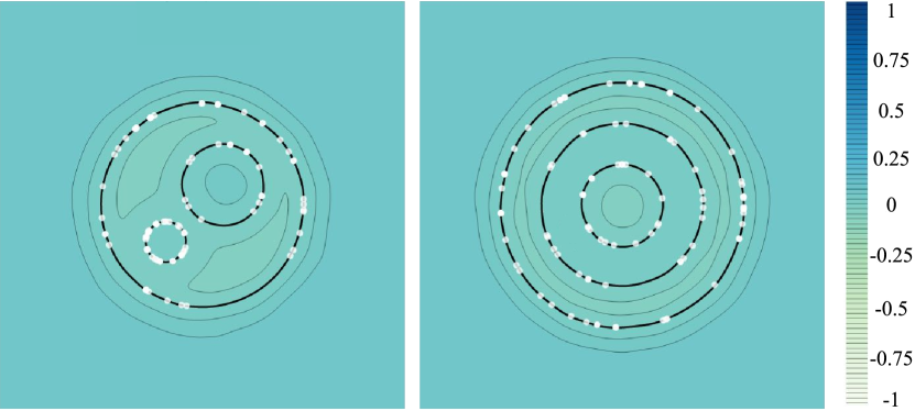
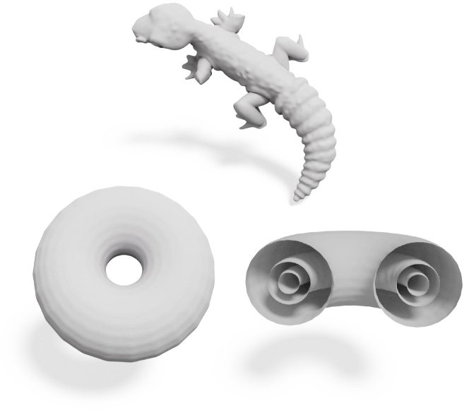
Our method supports nested surfaces with multiple connected components. For easy visualization, we present 2D cases in Fig. 19. Additionally, we present a 3D shape with several separate tori with different radii to demonstrate our expressive ability. We also visualize the gecko model in Fig. 20. Our method works in a coarse-to-fine fashion and can eventually recover the true topology even for multi-surface shapes.

Figure 21. Comparing ours (top) and DiGS (bottom) (Ben-Shabat et al., 2022) by observing the four intermediate iterations under high genus shape. The input is 100K points.

High-genus Shapes

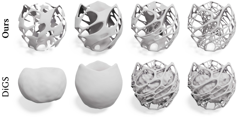
Fig. 21 shows the iteration process of our method comparison to DiGS (Ben-Shabat et al., 2022) for high-genus shapes. The input has 100K points with complex topology. DiGS cannot incorrectly close the holes of the shapes. Our method first suppresses the critical points that look forward to the coarse surface and then gradually recovers the real complex topology.

\begin{overpic}[width=433.62pt]{figures/abl_matrix.pdf} \par\put(15.0,-3.0){(a)} \par\put(37.0,-3.0){(b)} \par\put(60.0,-3.0){(c)} \par\put(83.0,-3.0){(d)} \end{overpic}

Figure 22. We test a point cloud of the genus-3 torus with different experimental configurations. From left to right: (a) Input, (b) $\lambda_{\text{singularH}}=3\&decay$, (c) $\lambda_{\text{singularH}}=3\&no-decay$, and (d) $\lambda_{\text{singularH}}=30\&no-decay$.

Varying Point Density, Data Sparsity, Noise

In Fig. 22, we used three-hole shapes to test our methods with different point cloud artifacts, including varying point density, data sparsity, and noise. By default, we used 8K points except for data sparsity validation. We show the results under three different configurations: $\lambda_{\text{singularH}}=3\&decay$, $\lambda_{\text{singularH}}=3\&no-decay$ and $\lambda_{\text{singularH}}=30\&no-decay$. We can observe that the default parameters $\lambda_{\text{singularH}}=3\&decay$ are robust to different point cloud artifacts. Additionally, large weights without decay are more robust to noisy and sparse inputs in terms of recovering the topology of the underlying shape, but they may yield over-smoothed results or deviate from the true surfaces.

Figure 23. The reconstruction results from sketch points by different methods.

Sketch Input

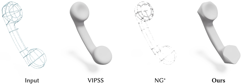
It is interesting to determine whether our approach can transform a super-sparse 3D sketch point cloud into a meaningful shape. In VIPSS (Huang et al., 2019), the authors provided a 3D sketch point cloud of approximately 1K points. We visualized the reconstructed results by VIPSS (Huang et al., 2019), NG (Huang et al., 2022a), and our method in Fig. 23. NG fails because its training set does not include sketch-type data. Our result is comparable to VIPSS, but VIPSS is severely limited by the number of points.

Figure 24. The error colormaps of the octa-flower (10K points) reconstructed by our method, Hessian energy, and DiGS (Ben-Shabat et al., 2022) indicate that our method has smaller error near sharp edges.

Sharp Features

We utilize the octa-flower model (comprising 10K points) to evaluate our method’s capacity to preserve sharp edges (as depicted in Fig. 24). The error colormaps demonstrate that our approach surpasses both the Hessian energy method and DiGS (Ben-Shabat et al., 2022), which employs Laplacian energy. The primary cause of their suboptimal performance is the smooth energy and original Eikonal condition, which result in gradient inaccuracies near sharp edges.

\begin{overpic}[width=433.62pt]{figures/KITTI.pdf} \par\put(15.0,-3.0){Input} \par\put(37.0,-3.0){OSP} \par\put(60.0,-3.0){DiGS} \par\put(83.0,-3.0){{Ours}} \end{overpic}

Figure 25. The visual comparison under KITTI (Geiger et al., 2012).

Appendix B Limitations

LiDAR Input.

In its present state, Neural-Singular-Hessian is not well-suited for processing LiDAR input with unique point distributions. Unlike the point clouds from DoF or structural light cameras, LiDAR has its unique distribution characteristics, which include stripe distribution, sparsity, and a substantial presence of missing parts. In particular, most data derived from the KITTI dataset are partial scans. This presents significant challenges in closing the gaps inherent between the stripes and completing large missing parts. Our results, in comparison with DiGS (Ben-Shabat et al., 2022) and OSP (Baorui et al., 2022a) (specifically designed to handle sparse point clouds), are presented in Fig. 25 within the context of the KITTI dataset (Geiger et al., 2012). Despite its advantages, our algorithm is unable to effectively process such data, resulting in discrepancies between different levels of points.

Figure 26. Scene-level reconstruction under 3DScene (Zhou and Koltun, 2013).

Scene-level Reconstruction

We also try our method to reconstruct the scene. We propose experiments under 3DScene (Zhou and Koltun, 2013) with 20K points for each scene. The results in Fig. 26 show that it seems existing methods leveraging sine activation function without normal are weak in handling scene data due to the planes (wall, floor). It is interesting to extend our method for scenes in the future.

Appendix C Experimental Details

C.1. Evaluation metrics

To compare the performance of different reconstruction methods, we use the same evaluation metrics as ConvONet (Songyou et al., 2020), i.e., Chamfer distances, F-Score, and Normal consistency. We denote $M_{g}$ and $M_{p}$ as the ground-truth mesh (or point cloud) and the mesh of the predicted result, respectively. Let $P_{1}$ and $P_{2}$ be the randomly sampled points on the ground-truth mesh (or point cloud) and the predicted mesh.

Chamfer Distance

The Chamfer distance between two point clouds $P_{1}$, $P_{2}$ is defined as follows:

(17) $$\operatorname{Chamfer}\left(P_{1},P_{2}\right)= \frac{1}{2|P1|}\sum_{p_{1}\in P_{1}}\min_{p_{2}\in P_{2}}d(p_{1},p_{2})$$

$$+\frac{1}{2|P2|}\sum_{p_{2}\in P_{2}}\min_{p_{1}\in P_{1}}d(p_{1},p_{2}),$$

where $d(p_{1},p_{2})$ is the straight-line distance between points $p1$, $p2$. We use the $L_{1}$ norm following ConvONet (Songyou et al., 2020).

F-Score.

The F-Score between the two point clouds $P_{1}$ and $P_{2}$ at a given threshold $t$ is given by:

(18) $$\operatorname{F-Score}\left(t,P_{1},P_{2}\right)=\frac{2\text{ Recall Precision }}{\text{ Recall }+\text{ Precision }},$$

where

(19) $$\operatorname{Recall}\left(t,P_{1},P_{2}\right)=\left|\left\{p_{1}\in P_{1}\text{, s.t. }\min_{p_{2}\in P_{2}}d\left(p_{1},p_{2}\right)<t\right\}\right|$$

$$\text{ Precision }\left(t,P_{1},P_{2}\right)=\left|\left\{p_{2}\in P_{2}\text{, s.t. }\min_{p_{1}\in P_{1}}d\left(p_{2},p_{1}\right)<t\right\}\right|$$

Normal consistency

The normal consistency between two point clouds $P_{1}$, $P_{2}$ is defined as follows:

(20) $$\mathrm{NormalC.}\left(P_{1},P_{2}\right)= \frac{1}{2|P1|}\sum_{p_{1}\in P_{1}}n_{p_{1}}\cdot n_{\text{closest }\left(p_{1},P_{2}\right)}$$

$$+\frac{1}{2|P2|}\sum_{p_{2}\in P_{2}}n_{p_{2}}\cdot n_{\text{closest }\left(p_{2},P_{1}\right)},$$

where

(21) $$\operatorname{closest}(p,P)=\underset{p^{\prime}\in P}{\arg\min}\ d\left(p,p^{\prime}\right)$$

C.2. Surface reconstruction on SRB

We report the results of baselines using their official source code. All methods leverage $256^{3}$ grids (SPSR (Kazhdan et al., 2013) and iPSR (Hou et al., 2022) use the octree of depth 8) to extract the final mesh. We trained DiGS and SIREN with four hidden layers, each layer containing 256 units, and the total number of iterations is set to 10K same as ours. More parameters of each method are used with their default settings.

In Tab. 13, we provide the relevant comparison statistics on the Surface Reconstruction Benchmark (Williams et al., 2019). It can be seen that our method achieves the best score on all the shapes except Daratech. Fig. 27 shows the visual comparison.

Table 13. Comparison on Surface Reconstruction Benchmark.

	Mean		Std.		Anchor		Daratech		DC		Gargoyle		Lord Quas
	Chamfer $\downarrow$	F-Score $\uparrow$	Chamfer	F-Score	Chamfer $\downarrow$	F-Score $\uparrow$	Chamfer $\downarrow$	F-Score $\uparrow$	Chamfer $\downarrow$	F-Score $\uparrow$	Chamfer $\downarrow$	F-Score $\uparrow$	Chamfer $\downarrow$	F-Score $\uparrow$
SPSR* (Kazhdan et al., 2013)	4.36	75.87	1.56	18.57	6.93	46.14	4.20	83.22	3.40	85.89	4.37	70.65	2.85	93.60
DGP* (Williams et al., 2019)	4.87	73.34	1.64	18.56	7.56	43.04	3.85	83.05	4.85	78.79	4.84	70.40	3.26	91.45
SIREN (Sitzmann et al., 2020)	18.24	38.74	17.09	31.26	38.31	5.05	6.19	52.30	46.24	75.47	35.50	7.25	6.53	54.58
SAP (Peng et al., 2021)	6.19	57.21	1.75	11.66	8.33	46.73	7.76	48.42	5.11	60.34	4.27	75.66	5.54	54.61
iPSR (Hou et al., 2022)	4.54	75.07	1.78	19.18	7.53	44.29	4.20	83.51	3.52	84.36	4.49	69.87	2.91	93.53
PCP (Baorui et al., 2022b)	6.53	47.97	1.75	14.50	9.04	37.63	7.23	36.08	5.82	45.09	6.17	49.71	4.30	72.09
CAP-UDF (Zhou et al., 2022)	4.54	74.75	1.82	18.84	7.68	43.92	3.96	82.78	3.61	84.03	4.40	70.82	3.06	92.19
DiGS (Ben-Shabat et al., 2022)	4.16	76.69	1.44	18.15	6.63	46.52	3.62	85.54	3.32	86.11	4.19	73.34	3.04	91.86
Ours	3.76	81.38	0.98	13.73	5.31	59.32	3.75	83.89	3.28	87.05	3.84	80.09	2.64	96.46

Figure 27. Visual comparison about various approaches on the Surface Reconstruction Benchmark dataset (Williams et al., 2019).

C.3. Surface reconstruction on ShapeNet

We report all baselines using their code. All methods leverage $256^{3}$ grids (SPSR (Kazhdan et al., 2013), iPSR (Hou et al., 2022), and PGR (Lin et al., 2022) use the octree of depth 8) to extract the final mesh. We trained DiGS and SIREN with four hidden layers, each layer containing 256 units. The total number of iterations is set to 10K. We conduct 10K iterations for DiGS and SIREN, the same as ours, and train SAL and IGR within 20K iterations and 15K iterations, respectively. For NSP (Williams et al., 2021), we follow the parameters used in its main paper (1024 input points with 1024 Nyström samples and no regularization) and set the Nyström samples to 1000 and 3000 for 1K and 3K input points, respectively, without regularization.For PGR, we use the officially recommended parameters for sparse inputs (alpha: 2, wmin: 0.04). For the supervision methods SAP (Peng et al., 2021) and POCO (Boulch and Marlet, 2022), we retrain them with 1K points and 3K points under ShapeNet (Chang et al., 2015), respectively. More parameters of each method follow the default setting.

Table 14. Class-by-class comparison of the surface reconstruction quality on 1K-point clouds of ShapeNet.

		airplane	bench	cabinet	car	chair	display	lamp	loudspeaker	rifle	sofa	table	telephone	watercraft	mean	std.
Normal C. $\uparrow$	SPSR∗ (Kazhdan et al., 2013)	90.79	87.45	92.86	91.30	90.14	94.32	91.06	93.79	94.18	91.58	88.97	96.87	91.46	91.89	4.76
	NSP∗ (Williams et al., 2021)	81.87	79.43	89.33	89.49	83.16	90.42	85.70	91.50	89.22	87.01	82.38	94.43	87.74	87.05	6.05
	SAL (Atzmon and Lipman, 2020)	75.33	73.27	89.04	88.55	75.20	88.61	79.65	93.75	80.43	85.85	73.44	92.25	82.12	82.99	11.11
	IGR (Gropp et al., 2020)	74.77	73.65	84.59	84.90	76.02	70.67	82.11	92.46	77.95	85.32	73.03	70.22	82.92	79.26	12.27
	SIREN (Sitzmann et al., 2020)	84.70	76.29	74.42	75.44	80.57	83.56	85.47	73.42	83.78	72.63	78.82	88.86	80.94	79.91	8.87
	DiGS (Ben-Shabat et al., 2022)	94.12	89.76	91.32	90.06	90.79	94.90	93.19	92.80	96.08	90.44	89.48	98.12	93.70	92.67	6.03
	OSP (Baorui et al., 2022a)	92.16	85.66	90.72	90.64	91.67	94.19	91.38	93.48	94.17	91.13	92.26	96.91	90.24	91.89	5.52
	iPSR (Hou et al., 2022)	83.41	78.82	91.28	89.93	83.86	89.47	88.94	92.72	92.87	88.73	79.62	94.00	88.61	87.88	7.26
	PGR (Lin et al., 2022)	83.16	83.91	91.80	90.25	88.21	93.24	88.06	93.29	89.36	91.02	87.13	95.92	88.54	89.53	5.35
	SAP+ (Peng et al., 2021)	94.52	92.53	96.17	92.41	95.17	97.35	93.46	95.15	95.22	95.41	95.66	98.44	92.51	94.92	3.60
	POCO+ (Boulch and Marlet, 2022)	93.65	91.96	96.20	91.29	95.23	97.38	93.18	95.06	95.91	95.77	95.59	98.62	92.45	94.79	4.15
	Ours	96.04	92.20	94.92	93.17	94.93	97.77	94.75	93.58	92.86	96.01	95.81	98.83	95.41	95.10	4.04
Chamfer $\downarrow$	SPSR∗ (Kazhdan et al., 2013)	6.09	10.29	9.63	9.53	12.34	9.81	10.35	9.05	3.50	10.52	14.26	6.33	9.86	9.35	7.66
	NSP∗ (Williams et al., 2021)	20.84	13.32	12.84	7.74	17.47	10.30	14.13	12.91	4.40	12.18	19.74	6.19	10.46	12.51	7.29
	SAL (Atzmon and Lipman, 2020)	64.90	56.83	25.53	20.98	92.43	30.14	99.07	20.59	38.40	28.57	71.88	24.37	36.80	47.46	50.57
	IGR (Gropp et al., 2020)	13.20	98.42	36.03	55.19	52.71	10.54	65.54	20.19	11.22	44.93	78.41	13.10	78.88	77.68	59.55
	SIREN (Sitzmann et al., 2020)	27.12	49.85	26.99	44.64	17.21	41.93	28.31	38.66	84.89	38.38	25.90	33.19	37.39	38.04	46.02
	DiGS (Ben-Shabat et al., 2022)	4.17	6.37	10.72	7.39	8.70	6.29	5.59	9.90	2.53	10.04	11.15	3.22	5.11	7.01	5.52
	OSP (Baorui et al., 2022a)	7.36	8.89	9.81	10.29	9.49	9.37	7.57	8.93	5.57	9.18	8.56	6.02	12.97	8.77	6.76
	iPSR (Hou et al., 2022)	13.98	21.38	10.82	11.03	18.84	12.56	11.93	10.34	3.95	13.65	22.76	7.31	12.41	13.16	11.78
	PGR	10.13	11.59	10.54	10.85	11.23	8.72	13.99	10.12	6.11	11.26	13.25	6.69	11.90	10.49	6.52
	SAP+ (Peng et al., 2021)	3.36	3.78	4.58	6.19	4.71	3.63	4.20	6.55	2.62	4.94	5.66	2.96	7.16	4.64	3.71
	POCO+ (Boulch and Marlet, 2022)	4.06	4.42	4.48	6.60	4.93	3.73	4.11	5.84	2.25	4.31	5.86	2.33	6.03	4.53	4.05
	Ours	2.66	4.06	5.57	4.68	5.25	3.36	3.45	9.19	2.44	4.28	4.69	2.34	3.33	4.26	3.11
F-Score $\uparrow$	SPSR∗ (Kazhdan et al., 2013)	54.28	36.69	39.63	49.11	34.55	38.94	51.89	44.16	76.85	38.52	23.76	71.35	50.08	46.91	26.06
	NSP∗ (Williams et al., 2021)	33.69	29.18	21.13	44.77	19.17	36.16	39.69	28.72	69.88	26.08	18.25	59.65	43.91	36.17	21.56
	SAL (Atzmon and Lipman, 2020)	6.79	9.88	20.30	24.47	7.92	24.92	8.48	23.80	13.67	25.31	7.04	53.29	23.07	18.16	19.15
	IGR (Gropp et al., 2020)	0.72	11.84	41.50	32.34	23.48	14.61	29.34	48.08	11.89	40.58	11.32	12.73	24.33	22.48	32.08
	SIREN (Sitzmann et al., 2020)	34.92	23.14	18.97	14.56	32.50	22.94	40.34	14.60	30.34	16.00	22.52	32.29	22.16	25.02	23.52
	DiGS (Ben-Shabat et al., 2022)	69.85	61.19	38.32	54.62	45.74	57.97	70.23	41.02	88.13	39.74	38.38	87.67	70.44	58.72	29.77
	OSP (Baorui et al., 2022a)	40.72	51.27	46.06	35.57	42.16	47.60	58.39	43.93	47.13	52.54	43.26	81.23	28.54	47.57	23.45
	iPSR (Hou et al., 2022)	27.35	24.04	32.92	43.52	24.99	33.81	50.28	39.66	72.93	35.79	18.29	64.51	43.37	39.36	25.11
	PGR (Lin et al., 2022)	35.49	30.33	35.22	40.82	31.70	37.00	34.25	38.51	52.15	29.30	22.80	65.87	35.51	37.61	19.14
	SAP+ (Peng et al., 2021)	82.48	78.55	70.19	67.54	72.31	80.75	77.30	51.80	88.26	73.05	54.48	93.69	65.10	73.50	25.02
	POCO+ (Boulch and Marlet, 2022)	78.56	74.93	74.35	68.06	72.23	83.71	80.48	60.07	91.82	77.32	57.29	94.48	68.97	75.56	26.46
	Ours	90.32	79.93	74.58	75.02	72.28	89.76	85.28	54.87	89.45	80.99	74.13	96.03	83.95	80.51	21.48

Figure 28. Visual comparison on ShapeNet (Chang et al., 2015), where the input has 1K points.

Table 15. Class-by-class comparison of the surface reconstruction quality on 3K-point clouds of ShapeNet.

		airplane	bench	cabinet	car	chair	display	lamp	loudspeaker	rifle	sofa	table	telephone	watercraft	mean	std.
Normal C. $\uparrow$	SPSR∗ (Kazhdan et al., 2013)	95.30	92.85	95.98	93.43	95.02	97.35	95.03	96.19	96.93	95.53	94.65	98.67	94.61	95.50	3.30
	NSP∗ (Williams et al., 2021)	86.04	85.37	91.30	91.08	87.83	93.70	90.45	92.95	94.94	90.18	87.66	96.87	91.30	90.74	5.48
	SAL (Atzmon and Lipman, 2020)	77.52	78.04	90.64	90.32	79.57	91.74	86.09	94.60	86.35	90.44	77.05	97.59	87.68	86.69	9.66
	IGR (Gropp et al., 2020)	74.48	73.98	88.47	86.00	75.23	76.79	83.46	92.61	78.43	82.07	73.97	82.29	83.22	80.85	11.88
	SIREN (Sitzmann et al., 2020)	88.42	80.93	78.58	77.01	84.08	89.76	84.80	78.84	84.98	80.28	86.70	90.27	84.30	83.79	10.20
	DiGS (Ben-Shabat et al., 2022)	97.19	93.86	94.61	93.18	93.98	97.50	95.59	96.05	98.12	96.11	94.18	99.02	96.28	95.82	4.44
	OSP (Baorui et al., 2022a)	94.97	91.87	95.23	92.90	95.44	97.56	93.00	95.63	92.62	95.70	95.90	97.51	93.23	94.73	3.94
	iPSR (Hou et al., 2022)	92.45	88.80	93.26	92.51	92.64	95.35	93.70	94.54	96.39	92.41	89.66	97.56	92.63	93.22	5.26
	PGR (Lin et al., 2022)	85.57	86.85	94.09	91.25	91.88	95.59	90.63	95.17	91.14	93.55	91.03	97.80	90.19	91.90	4.93
	SAP+ (Peng et al., 2021)	96.10	94.26	97.36	93.79	96.93	98.01	95.35	96.84	96.14	97.34	97.09	99.05	94.01	96.33	3.24
	POCO+ (Boulch and Marlet, 2022)	96.81	94.23	97.28	93.52	96.56	98.29	95.92	96.86	97.56	96.87	96.65	99.02	93.77	96.41	3.53
	Ours	97.62	94.77	97.24	94.97	97.61	98.53	96.53	96.24	96.34	97.81	98.03	99.32	96.70	97.05	2.91
Chamfer $\downarrow$	SPSR∗ (Kazhdan et al., 2013)	2.73	4.08	5.06	6.66	5.83	4.08	3.97	6.26	1.73	5.31	6.00	2.36	6.50	4.66	4.64
	NSP∗ (Williams et al., 2021)	19.44	7.61	9.57	6.07	11.75	7.08	7.33	13.65	2.45	8.24	10.14	3.82	7.96	8.85	6.96
	SAL (Atzmon and Lipman, 2020)	52.97	45.43	21.19	14.25	55.97	23.83	34.35	13.93	13.33	17.25	68.27	6.54	23.29	29.98	31.86
	IGR (Gropp et al., 2020)	12.44	69.77	34.50	24.30	58.89	91.40	55.51	19.87	68.71	46.77	75.63	83.02	60.22	62.54	48.44
	SIREN (Sitzmann et al., 2020)	26.12	38.23	33.62	42.33	23.52	17.84	46.18	34.34	65.53	23.49	21.36	30.22	42.08	34.19	46.77
	DiGS (Ben-Shabat et al., 2022)	2.44	3.87	8.50	4.82	7.69	4.45	3.83	5.95	1.35	4.50	6.63	2.36	3.23	4.59	4.94
	OSP (Baorui et al., 2022a)	5.85	4.40	6.02	9.28	5.97	4.20	11.91	6.63	9.09	5.09	5.74	5.15	9.06	6.80	6.61
	iPSR (Hou et al., 2022)	4.17	6.08	6.35	7.22	6.97	5.40	4.27	7.20	2.10	7.28	7.81	4.60	7.84	5.95	5.97
	PGR (Lin et al., 2022)	7.27	8.17	7.19	8.41	7.69	6.22	8.52	7.78	4.93	7.45	8.85	3.70	9.28	7.34	4.81
	SAP+ (Peng et al., 2021)	2.63	2.82	3.79	5.89	3.78	3.46	3.40	4.76	2.37	3.11	4.13	2.07	6.48	3.75	4.16
	POCO+ (Boulch and Marlet, 2022)	2.00	3.64	3.76	5.30	4.02	2.93	2.47	4.13	1.37	3.91	4.99	2.18	6.40	3.62	4.21
	Ours	1.84	2.61	3.59	3.61	3.77	2.84	2.34	7.46	1.35	2.97	2.93	1.84	2.90	3.08	2.64
F-Score $\uparrow$	SPSR∗ (Kazhdan et al., 2013)	90.17	76.96	67.50	69.99	65.21	81.29	79.09	56.36	95.66	70.81	61.00	94.69	69.64	75.28	25.76
	NSP∗ (Williams et al., 2021)	50.61	46.86	38.65	57.83	30.18	54.11	60.14	28.52	91.31	44.29	33.47	81.70	63.80	52.42	28.55
	SAL (Atzmon and Lipman, 2020)	8.73	15.46	24.86	34.22	11.06	23.62	26.27	31.98	28.40	30.07	8.37	62.90	29.98	25.76	22.43
	IGR (Gropp et al., 2020)	1.77	10.28	56.52	47.66	12.76	15.74	31.11	60.90	4.44	34.99	14.17	21.77	29.49	26.28	35.91
	SIREN (Sitzmann et al., 2020)	45.30	29.34	17.52	15.28	39.76	45.30	42.28	16.07	44.51	22.96	26.04	47.63	27.59	32.34	30.13
	DiGS (Ben-Shabat et al., 2022)	93.08	83.44	53.57	77.66	68.33	77.55	85.41	62.75	98.57	76.56	68.14	95.84	84.40	78.87	27.34
	OSP (Baorui et al., 2022a)	43.02	73.47	65.35	38.96	57.37	80.52	57.39	55.29	41.30	75.01	61.78	84.08	35.03	59.12	25.82
	iPSR (Hou et al., 2022)	72.59	62.60	58.69	66.97	59.01	73.75	80.01	53.79	93.43	62.92	50.46	91.29	64.98	68.42	26.36
	PGR (Lin et al., 2022)	44.70	42.12	46.98	57.14	46.95	57.69	48.46	50.78	62.57	43.66	38.29	84.75	44.64	51.44	23.12
	SAP+ (Peng et al., 2021)	91.88	90.83	82.41	75.20	83.54	90.65	87.47	68.85	91.63	88.56	81.13	98.21	71.93	84.79	20.94
	POCO+ (Boulch and Marlet, 2022)	96.21	82.62	81.33	82.85	83.37	93.08	93.74	72.98	99.30	83.13	71.51	95.31	74.99	85.42	33.13
	Ours	98.75	93.13	89.08	85.80	86.56	94.42	92.12	74.05	97.69	91.17	89.79	99.49	87.21	90.71	16.28

Figure 29. Visual comparison the ShapeNet (Chang et al., 2015), where the input has 3K points.

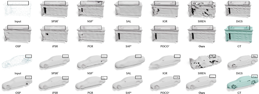
We give the comparison statistics under the settings of 1K points and 3K points in Tab. 14 and Tab. 15, respectively. The corresponding visual comparison is given in Fig. 28 and Fig. 29, respectively. Both qualitative and quantitative comparisons show that our method can faithfully recover fine geometric details and thin structures, outperforming the other methods.

C.4. Surface Reconstruction on ABC and Thingi10K

We report the results of baselines using their source code. All methods leverage $256^{3}$ grids, and SPSR (Kazhdan et al., 2013), iPSR (Hou et al., 2022), PGR (Lin et al., 2022), and Neural Galerkin (Huang et al., 2022a) use the depth 8 during the mesh extraction phase. For SAL (Atzmon and Lipman, 2020) and IGR (Gropp et al., 2020), we trained them with 20K iterations and 15K iterations, respectively. We conduct 10K iterations for DiGS and SIREN, the same as ours, where the SIREN network has four hidden layers, each containing 256 neurons. For PGR, we use the officially recommended parameters for the 10K-point input (alpha: 1.2, wk: 16). For the supervision methods POCO (Boulch and Marlet, 2022) and Neural Galerkin (Huang et al., 2022a) (without normals), we retrained them with 10K points under ShapeNet (Chang et al., 2015) to validate their generalization ability. Other parameters remain the same with the default settings.

We show the visual comparison of different approaches on ABC (Koch et al., 2019) with 10K points in Fig. 30 and Fig. 31. The comparison shows that Our method is better at recovering thin geometry features and can achieve a good trade-off between smoothness and feature preservation.

Figure 30. Visual comparison about different approaches on ABC (Koch et al., 2019) with 10K points. Our method is better at recovering thin geometry features.

Figure 31. Visual comparison about different approaches on Thingi10K (Koch et al., 2019) with 10K points. Our method achieves a good trade-off between smoothness and feature preservation.

C.5. Real Scans

We report the results of baselines using their source code. Among them, the supervised method Neural Galerkin (Huang et al., 2022a) (without normals), and we retrained them with 10K points under ShapeNet (Chang et al., 2015) to validate its generality. All methods leverage $256^{3}$ grids to extract the mesh. We conduct 10K iterations for DiGS (Ben-Shabat et al., 2022), PCP (Baorui et al., 2022b), and ours. Other parameters remain the same with the default settings.

C.6. Large Scans

We report the results of baselines using their source code. All methods leverage $512^{3}$ grids to extract the mesh. We conduct 50K iterations for DiGS and SIREN, where the SIREN network has four hidden layers, each containing 256 neurons, the same as ours, For the supervision method Neural Galerkin (Huang et al., 2022a) (without normals), we retrained them with 10K points under ShapeNet (Chang et al., 2015) to validate its generality. Other parameters remain the same with the default settings.

The quantitative comparison statistics are reported in Tab. 16, while the visual comparison is available in Fig. 33.

C.7. Shape Space Learning

Shape space learning requires training a single model to learn to represent multiple shapes from a class of related shapes, which is more challenging than the single overfitting shape. For the encoder, we adopt the encoder from Convolutional Occupancy Network (Songyou et al., 2020). Specifically, we project the sparse on-surface point features obtained using a modified PointNet (Qi et al., 2017) onto a regular 3D grid, then use a convolutional module to propagate sparse on-surface point features to the off-surface area, and finally obtain the query feature using bilinear interpolation. For the decoder, we use the SIREN network has three hidden layers. Further, we adopt the FiLM conditioning (Chan et al., 2021) that applies an affine transformation to the network’s intermediate features as SIREN is weak in handling high-dimensional inputs (Chan et al., 2021; Mehta et al., 2021). We train our models for 200 epochs using AMSGrad optimizer (Reddi et al., 2018) with an initial learning rate of 0.0001 and decay to 0.000001 using cosine annealing (Loshchilov and Hutter, 2017). We divided the training set into mini-batches: a batch contains 32 different shapes (accumulate batches), where each shape is randomly sampled to produce 10K points. The experiments are conducted with 8 RTX 3090 graphics cards. In the inference stage, we fine-tune the whole network to perform high-fidelity surface reconstruction for each shape 3000 iterations utilizing our loss without the critical term inspired by SA-ConvNet (Tang et al., 2021b).

For baselines, we use the pre-trained model of IGR (Gropp et al., 2020), SAL (Atzmon and Lipman, 2020), SALD (Atzmon and Lipman, 2021), DualOctreeGNN (Wang et al., 2022) and DiGS (Ben-Shabat et al., 2022), and retrained the IGR and DualOctreeGNN for the version without normals supervision. We optimize DiGS (Ben-Shabat et al., 2022) in the inference stage with 3000 iterations for auto-decoder looking forward to better performance.

The visual comparison of different approaches on the DFAUST (Bogo et al., 2017) dataset is available in Fig. 32.

Figure 32. Visual comparison of shape space learning on DFAUST (Bogo et al., 2017). Our method can get reliable results without supervision and normals.

Figure 33. Visual comparison of different approaches on ThreedScans (Laric, 2012) with 10K points. Our method is comparable to the “with normals” version of SIREN.

Table 16. Quantitative comparison on the shapes from (Laric, 2012).

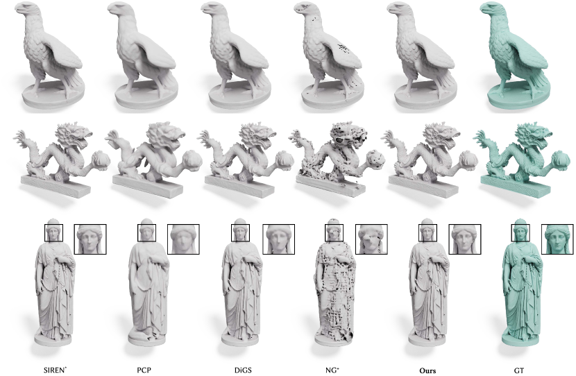
	Mean			Std.			Eagle			Dragon			Hosmer
	Normal C. $\uparrow$	Chamfer $\downarrow$	F-Score $\uparrow$	Normal C.	Chamfer	F-Score	Normal C. $\uparrow$	Chamfer $\downarrow$	F-Score $\uparrow$	Normal C. $\uparrow$	Chamfer $\downarrow$	F-Score $\uparrow$	Normal C. $\uparrow$	Chamfer $\downarrow$	F-Score $\uparrow$
SIREN* (Sitzmann et al., 2020)	98.38	0.96	63.61	0.30	0.17	19.62	98.74	1.16	42.55	98.21	0.84	81.40	98.21	0.87	66.89
PCP (Baorui et al., 2022b)	94.32	4.44	11.83	2.58	1.41	9.41	97.27	3.01	12.00	93.16	5.83	2.33	92.51	4.47	21.15
DiGS (Ben-Shabat et al., 2022)	97.41	0.92	63.78	0.62	0.22	21.91	98.08	1.10	42.24	97.31	0.67	86.06	96.84	0.98	63.04
NG (Huang et al., 2022a)	85.97	3.02	31.01	9.10	2.09	20.67	95.89	1.43	46.66	77.99	5.39	7.57	84.03	2.24	38.79
Ours	98.44	0.74	79.77	0.15	0.09	9.90	98.53	0.84	69.39	98.53	0.66	89.12	98.26	0.73	80.81

References

- (1)
- Atzmon and Lipman (2020) Matan Atzmon and Yaron Lipman. 2020. SAL: Sign Agnostic Learning of Shapes From Raw Data. In Proceedings of the IEEE/CVF Conference on Computer Vision and Pattern Recognition (CVPR).
- Atzmon and Lipman (2021) Matan Atzmon and Yaron Lipman. 2021. SALD: Sign Agnostic Learning with Derivatives. In International Conference on Learning Representations (ICLR).
- Audin et al. (2014) Michele Audin, Mihai Damian, and Reinie Erné. 2014. Morse theory and Floer homology. Springer.
- Baorui et al. (2022b) Ma Baorui, Liu Yu-Shen, Zwicker Matthias, and Han Zhizhong. 2022b. Surface Reconstruction from Point Clouds by Learning Predictive Context Priors. In Proceedings of the IEEE/CVF Conference on Computer Vision and Pattern Recognition (CVPR).
- Baorui et al. (2022a) Ma Baorui, Liu Yu-Shen, and Han Zhizhong. 2022a. Reconstructing Surfaces for Sparse Point Clouds with On-Surface Priors. In Proceedings of the IEEE/CVF Conference on Computer Vision and Pattern Recognition (CVPR).
- Baorui et al. (2021) Ma Baorui, Han Zhizhong, Liu Yu-Shen, and Zwicker Matthias. 2021. Neural-Pull: Learning Signed Distance Functions from Point Clouds by Learning to Pull Space onto Surfaces. In Proceedings of the International Conference on Machine Learning (ICML).
- Ben-Shabat et al. (2022) Yizhak Ben-Shabat, Chamin Hewa Koneputugodage, and Stephen Gould. 2022. DiGS: Divergence guided shape implicit neural representation for unoriented point clouds. In Proceedings of the IEEE/CVF Conference on Computer Vision and Pattern Recognition (CVPR).
- Bogo et al. (2017) Federica Bogo, Javier Romero, Gerard Pons-Moll, and Michael J. Black. 2017. Dynamic FAUST: Registering Human Bodies in Motion. In Proceedings IEEE Conf. on Computer Vision and Pattern Recognition (CVPR).
- Boulch and Marlet (2022) Alexandre Boulch and Renaud Marlet. 2022. POCO: Point Convolution for Surface Reconstruction. In Proceedings of the IEEE/CVF Conference on Computer Vision and Pattern Recognition (CVPR).
- Calakli and Taubin (2011) Fatih Calakli and Gabriel Taubin. 2011. SSD: Smooth Signed Distance Surface Reconstruction. Computer Graphics Forum 30, 7 (2011), 1993–2002.
- Carr et al. (2001) Jonathan C Carr, Richard K Beatson, Jon B Cherrie, Tim J Mitchell, W Richard Fright, Bruce C McCallum, and Tim R Evans. 2001. Reconstruction and representation of 3D objects with radial basis functions. In Proceedings of the 28th annual conference on Computer graphics and interactive techniques.
- Chabra et al. (2020) Rohan Chabra, Jan E Lenssen, Eddy Ilg, Tanner Schmidt, Julian Straub, Steven Lovegrove, and Richard Newcombe. 2020. Deep Local Shapes: Learning local sdf priors for detailed 3d reconstruction. In Computer Vision–ECCV 2020: 16th European Conference, Glasgow, UK, August 23–28, 2020, Proceedings, Part XXIX 16. Springer, 608–625.
- Chan et al. (2021) Eric Chan, Marco Monteiro, Petr Kellnhofer, Jiajun Wu, and Gordon Wetzstein. 2021. pi-GAN: Periodic Implicit Generative Adversarial Networks for 3D-Aware Image Synthesis. In Proceedings IEEE Conf. on Computer Vision and Pattern Recognition (CVPR).
- Chang et al. (2015) Angel X. Chang, Thomas Funkhouser, Leonidas Guibas, Pat Hanrahan, Qixing Huang, Zimo Li, Silvio Savarese, Manolis Savva, Shuran Song, Hao Su, Jianxiong Xiao, Li Yi, and Fisher Yu. 2015. ShapeNet: An Information-Rich 3D Model Repository. Technical Report arXiv:1512.03012 [cs.GR].
- Chibane et al. (2020) Julian Chibane, Aymen Mir, and Gerard Pons-Moll. 2020. Neural Unsigned Distance Fields for Implicit Function Learning. In Advances in Neural Information Processing Systems (NeurIPS).
- Erler et al. (2020) Philipp Erler, Paul Guerrero, Stefan Ohrhallinger, Niloy J Mitra, and Michael Wimmer. 2020. Points2surf: learning implicit surfaces from point clouds. In Proceedings of the European Conference on Computer Vision (ECCV).
- Geiger et al. (2012) Andreas Geiger, Philip Lenz, and Raquel Urtasun. 2012. Are we ready for Autonomous Driving? The KITTI Vision Benchmark Suite. In Conference on Computer Vision and Pattern Recognition (CVPR).
- Gropp et al. (2020) Amos Gropp, Lior Yariv, Niv Haim, Matan Atzmon, and Yaron Lipman. 2020. Implicit Geometric Regularization for Learning Shapes. In Proceedings of the International Conference on Machine Learning (ICML).
- Hoppe et al. (1992) Hugues Hoppe, Tony DeRose, Tom Duchamp, John Alan McDonald, and Werner Stuetzle. 1992. Surface reconstruction from unorganized points. Proceedings of the 19th annual conference on Computer graphics and interactive techniques.
- Hou et al. (2022) Fei Hou, Chiyu Wang, Wencheng Wang, Hong Qin, Chen Qian, and Ying He. 2022. Iterative Poisson Surface Reconstruction (IPSR) for Unoriented Points. ACM Trans. Graph. 41, 4 (2022), 13 pages.
- Huang et al. (2022a) Jiahui Huang, Hao-Xiang Chen, and Shi-Min Hu. 2022a. A Neural Galerkin Solver for Accurate Surface Reconstruction. ACM Trans. Graph. 41, 6 (2022), 16 pages.
- Huang et al. (2019) Zhiyang Huang, Nathan Carr, and Tao Ju. 2019. Variational Implicit Point Set Surfaces. ACM Trans. Graph. 38, 4 (2019), 13 pages.
- Huang et al. (2022b) Zhangjin Huang, Yuxin Wen, Zihao Wang, Jinjuan Ren, and Kui Jia. 2022b. Surface Reconstruction from Point Clouds: A Survey and a Benchmark. arXiv:arXiv:2205.02413
- Jiang et al. (2020) Chiyu Jiang, Avneesh Sud, Ameesh Makadia, Jingwei Huang, Matthias Nießner, Thomas Funkhouser, et al. 2020. Local implicit grid representations for 3d scenes. In Proceedings of the IEEE/CVF Conference on Computer Vision and Pattern Recognition (CVPR).
- Jin et al. (2020) Yiwei Jin, Diqiong Jiang, and Ming Cai. 2020. 3D reconstruction using deep learning: a survey. Commun. Inf. Syst. (2020).
- Kazhdan et al. (2013) Kazhdan, Fei Hou, Chiyu Wang, Wencheng Wang, Hong Qin, Chen Qian, and Ying He. 2013. Screened Poisson surface reconstruction. ACM Trans. Graph. 32, 3 (2013), 13 pages.
- Kazhdan et al. (2020) Misha Kazhdan, Ming Chuang, Szymon M. Rusinkiewicz, and Hugues Hoppe. 2020. Poisson Surface Reconstruction with Envelope Constraints. Computer Graphics Forum 30, 7 (2020), 1993–2002.
- Kazhdan et al. (2006) Michael M. Kazhdan, Matthew Bolitho, and Hugues Hoppe. 2006. Poisson surface reconstruction. In Eurographics Symposium on Geometry Processing.
- Kingma and Ba (2014) Diederik P. Kingma and Jimmy Ba. 2014. Adam: A Method for Stochastic Optimization.
- Koch et al. (2019) Sebastian Koch, Albert Matveev, Zhongshi Jiang, Francis Williams, Alexey Artemov, Evgeny Burnaev, Marc Alexa, Denis Zorin, and Daniele Panozzo. 2019. ABC: A Big CAD Model Dataset For Geometric Deep Learning. In Proceedings of the IEEE/CVF Conference on Computer Vision and Pattern Recognition (CVPR).
- Kolluri (2008) Ravikrishna Kolluri. 2008. Provably good moving least squares. ACM Transactions on Algorithms (TALG) (2008).
- Laric (2012) Oliver Laric. 2012. Three D Scans. http://threedscans.com/info/.
- Lewiner et al. (2003) Thomas Lewiner, Hélio Lopes, Antônio Wilson Vieira, and Geovan Tavares. 2003. Efficient implementation of marching cubes’ cases with topological guarantees. Journal of Graphics Tools 8, 2 (2003), 1–15.
- Li et al. (2016) Manyi Li, Falai Chen, Wenping Wang, and Changhe Tu. 2016. Sparse RBF surface representations. Computer Aided Geometric Design 48 (2016), 49–59.
- Lin et al. (2022) Siyou Lin, Dong Xiao, Zuoqiang Shi, and Bin Wang. 2022. Surface Reconstruction from Point Clouds without Normals by Parametrizing the Gauss Formula. ACM Trans. Graph. 42, 2 (2022), 19 pages.
- Lipman (2021) Yaron Lipman. 2021. Phase Transitions, Distance Functions, and Implicit Neural Representations. In Proceedings of the International Conference on Machine Learning (ICML).
- Loshchilov and Hutter (2017) Ilya Loshchilov and Frank Hutter. 2017. SGDR: Stochastic Gradient Descent with Warm Restarts. In International Conference on Learning Representations (ICLR).
- Mayost (2014) Daniel Mayost. 2014. Applications of the signed distance function to surface geometry. University of Toronto (Canada).
- Mehta et al. (2021) Ishit Mehta, Michael Gharbi, Connelly Barnes, Eli Shechtman, Ravi Ramamoorthi, and Manmohan Chandraker. 2021. Modulated Periodic Activations for Generalizable Local Functional Representations. In Proceedings of the IEEE/CVF International Conference on Computer Vision (ICCV).
- Mescheder et al. (2019) Lars Mescheder, Michael Oechsle, Michael Niemeyer, Sebastian Nowozin, and Andreas Geiger. 2019. Occupancy Networks: Learning 3D Reconstruction in Function Space. In Proceedings of the IEEE/CVF Conference on Computer Vision and Pattern Recognition (CVPR).
- Ohtake et al. (2003) Yutaka Ohtake, Alexander G. Belyaev, Marc Alexa, Greg Turk, and Hans-Peter Seidel. 2003. Multi-level partition of unity implicits. ACM SIGGRAPH 2005 Courses (2003).
- O’Neill (2006) Barrett O’Neill. 2006. Chapter 5 - Shape Operators. In Elementary Differential Geometry (Second Edition) (second edition ed.), Barrett O’Neill (Ed.). Academic Press, Boston, 202–262.
- Öztireli et al. (2009) A Cengiz Öztireli, Gael Guennebaud, and Markus Gross. 2009. Feature preserving point set surfaces based on non-linear kernel regression. In Computer Graphics Forum.
- Park et al. (2019) Jeong Joon Park, Peter Florence, Julian Straub, Richard Newcombe, and Steven Lovegrove. 2019. DeepSDF: Learning Continuous Signed Distance Functions for Shape Representation. In Proceedings of the IEEE/CVF Conference on Computer Vision and Pattern Recognition (CVPR).
- Peng et al. (2021) Songyou Peng, Chiyu ”Max” Jiang, and Yiyi Liao. 2021. Shape As Points: A Differentiable Poisson Solver. In Advances in Neural Information Processing Systems (NeurIPS).
- Qi et al. (2017) Charles R. Qi, Hao Su, Kaichun Mo, and Leonidas J. Guibas. 2017. PointNet: Deep Learning on Point Sets for 3D Classification and Segmentation. In Proceedings IEEE Conf. on Computer Vision and Pattern Recognition (CVPR).
- Reddi et al. (2018) Sashank J. Reddi, Satyen Kale, and Sanjiv Kumar. 2018. On the Convergence of Adam and Beyond. In International Conference on Learning Representations (ICLR).
- Sagun et al. (2017) Levent Sagun, Utku Evci, V Ugur Guney, Yann Dauphin, and Leon Bottou. 2017. Empirical analysis of the hessian of over-parametrized neural networks. arXiv preprint arXiv:1706.04454 (2017).
- Schroers et al. (2014) C. Schroers, S. Setzer, and J. Weickert. 2014. A Variational Taxonomy for Surface Reconstruction from Oriented Points. Computer Graphics Forum 33, 5 (2014), 195–204.
- Sellán and Jacobson (2022) Silvia Sellán and Alec Jacobson. 2022. Stochastic Poisson Surface Reconstruction. ACM Transactions on Graphics (TOG) (2022).
- Shen et al. (2004) Chen Shen, James F. O’Brien, and Jonathan R. Shewchuk. 2004. Interpolating and Approximating Implicit Surfaces from Polygon Soup. In ACM SIGGRAPH 2004 Papers.
- Sitzmann et al. (2020) Vincent Sitzmann, Julien N.P. Martel, Alexander W. Bergman, David B. Lindell, and Gordon Wetzstein. 2020. Implicit Neural Representations with Periodic Activation Functions. In Advances in Neural Information Processing Systems (NeurIPS).
- Songyou et al. (2020) Peng Songyou, Niemeyer Michael, Mescheder Lars, Pollefeys Marc, and Andreas Geiger. 2020. Convolutional Occupancy Networks. In Proceedings of the European Conference on Computer Vision (ECCV).
- Sulzer et al. (2023) Raphael Sulzer, Loic Landrieu, Renaud Marlet, and Bruno Vallet. 2023. A Survey and Benchmark of Automatic Surface Reconstruction from Point Clouds.
- Tang et al. (2021b) Jiapeng Tang, Jiabao Lei, Dan Xu, Feiying Ma, Kui Jia, and Lei Zhang. 2021b. SA-ConvONet: Sign-Agnostic Optimization of Convolutional Occupancy Networks. In Proceedings of the IEEE/CVF International Conference on Computer Vision.
- Tang et al. (2021a) Jia-Heng Tang, Weikai Chen, jie Yang, Bo Wang, Songrun Liu, Bo Yang, and Lin Gao. 2021a. OctField: Hierarchical Implicit Functions for 3D Modeling. In Advances in Neural Information Processing Systems (NeurIPS).
- van der Walt et al. (2014) Stéfan van der Walt, Johannes L. Schönberger, Juan Nunez-Iglesias, François Boulogne, Joshua D. Warner, Neil Yager, Emmanuelle Gouillart, Tony Yu, and the scikit-image contributors. 2014. scikit-image: image processing in Python. PeerJ 2 (2014), e453.
- Vizzo et al. (2021) Ignacio Vizzo, Xieyuanli Chen, Nived Chebrolu, Jens Behley, and Cyrill Stachniss. 2021. Poisson Surface Reconstruction for LiDAR Odometry and Mapping. In IEEE International Conference on Robotics and Automation (ICRA).
- Wang et al. (2022) Peng-Shuai Wang, Yang Liu, and Xin Tong. 2022. Dual Octree Graph Networks for Learning Adaptive Volumetric Shape Representations. ACM Trans. Graph. 41, 4 (2022), 15 pages.
- Williams et al. (2019) Francis Williams, Teseo Schneider, Claudio Silva, Denis Zorin, Joan Bruna, and Daniele Panozzo. 2019. Deep geometric prior for surface reconstruction. In Proceedings of the IEEE/CVF Conference on Computer Vision and Pattern Recognition (CVPR). IEEE.
- Williams et al. (2021) Francis Williams, Matthew Trager, Joan Bruna, and Denis Zorin. 2021. Neural splines: Fitting 3d surfaces with infinitely-wide neural networks. In Proceedings of the IEEE/CVF Conference on Computer Vision and Pattern Recognition (CVPR).
- Xu et al. (2023) Rui Xu, Zhiyang Dou, Ningna Wang, Shiqing Xin, Shuangmin Chen, Mingyan Jiang, Xiaohu Guo, Wenping Wang, and Changhe Tu. 2023. Globally Consistent Normal Orientation for Point Clouds by Regularizing the Winding-Number Field. ACM Transactions on Graphics (TOG) (2023).
- Xu et al. (2022) Rui Xu, Zixiong Wang, Zhiyang Dou, Chen Zong, Shiqing Xin, Mingyan Jiang, Tao Ju, and Changhe Tu. 2022. RFEPS: Reconstructing Feature-line Equipped Polygonal Surface. ACM Transactions on Graphics (TOG) (2022), 15 pages. https://doi.org/10.1145/3550454.3555443
- Ye et al. (2022) Jianglong Ye, Yuntao Chen, Naiyan Wang, and Xiaolong Wang. 2022. GIFS: Neural Implicit Function for General Shape Representation. In Proceedings of the IEEE/CVF Conference on Computer Vision and Pattern Recognition (CVPR).
- Yifan et al. (2021) Wang Yifan, Lukas Rahmann, and Olga Sorkine-hornung. 2021. Geometry-Consistent Neural Shape Representation with Implicit Displacement Fields. In International Conference on Learning Representations (ICLR).
- Yifan et al. (2020) Wang Yifan, Shihao Wu, Cengiz Oztireli, and Olga Sorkine-Hornung. 2020. Iso-Points: Optimizing Neural Implicit Surfaces with Hybrid Representations. In Proceedings of the IEEE/CVF Conference on Computer Vision and Pattern Recognition (CVPR).
- Zhang et al. (2022) Jingyang Zhang, Yao Yao, Shiwei Li, Tian Fang, David McKinnon, Yanghai Tsin, and Long Quan. 2022. Critical regularizations for neural surface reconstruction in the wild. In Proceedings of the IEEE/CVF Conference on Computer Vision and Pattern Recognition. 6270–6279.
- Zhou et al. (2022) Junsheng Zhou, Baorui Ma, Liu Yu-Shen, Fang Yi, and Han Zhizhong. 2022. Learning Consistency-Aware Unsigned Distance Functions Progressively from Raw Point Clouds. In Advances in Neural Information Processing Systems (NeurIPS).
- Zhou and Jacobson (2016) Qingnan Zhou and Alec Jacobson. 2016. Thingi10K: A Dataset of 10,000 3D-Printing Models. arXiv preprint arXiv:1605.04797 (2016).
- Zhou and Koltun (2013) Qian-Yi Zhou and Vladlen Koltun. 2013. Dense scene reconstruction with points of interest. ACM Trans. Graph. 32, 4 (2013).