Evolution of Chemistry in the envelope of Hot Corinos (ECHOS)

Abstract

Context. Within the project Evolution of Chemistry in the envelope of HOt corinoS (ECHOS), we present a study of sulphur chemistry in the envelope of the Class 0 source B 335 through observations in the spectral range $\lambda$ = 7, 3, and 2 mm.

Aims. Our goal is to characterise the sulphur chemistry in this isolated protostellar source and compare it with other Class 0 objects to determine the environmental and evolutionary effects on the sulphur chemistry in these young sources.

Methods. We have modelled observations and computed column densities assuming local thermodynamic equilibrium (LTE) and large velocity gradient (LVG) approximation. We have also used the code Nautilus to study the time evolution of sulphur species, as well as of several sulphur molecular ratios.

Results. We have detected 20 sulphur species in B 335 with a total gas-phase S abundance similar to that found in the envelopes of other Class 0 objects, but with significant differences in the abundances between sulphur carbon chains and sulphur molecules containing oxygen and nitrogen. Our results highlight the nature of B 335 as a source especially rich in sulphur carbon chains unlike other Class 0 sources. The low presence or absence of some molecules, such as SO and SO⁺, suggests a chemistry not particularly influenced by shocks. We, however, detect a large presence of HCS⁺ that, together with the low rotational temperatures obtained for all the S species ($<$15 K), reveals the moderate or low density of the envelope of B 335. Model results also show the large influence of the cosmic ray ionisation rate and density variations on the abundances of some S species (e.g. SO, SO₂, CCS, and CCCS) with differences of up to $\sim$4 orders of magnitude. We also find that observations are better reproduced by models with a sulphur depletion factor of 10 with respect to the sulphur cosmic elemental abundance.

Conclusions. The comparison between our model and observational results for B 335 reveals an age of 10⁴$<$$t$$<$10⁵ yr, which highlights the particularly early evolutionary stage of this source. B 335 presents a different chemistry compared to other young protostars that have formed in dense molecular clouds, which could be the result of accretion of surrounding material from the diffuse cloud onto the protostellar envelope of B 335. In addition, the theoretical analysis and comparison with observations of the SO₂/C₂S, SO/CS, and HCS⁺/CS ratios within a sample of prestellar cores and Class 0 objects show that they could be used as good chemical evolutionary indicators of the prestellar to protostellar transition.

1 Introduction

Hot corinos are regions that arise during the formation of solar-type protostars. The progressive collapse of a prestellar core leads to the heating of the infalling envelope of dust and gas to temperatures of hundreds of Kelvin, while the densities increase up to $\sim$10⁸-10⁹ cm^-3 in the inner $\sim$100 au around the central protostar. These are also the scales at which protoplanetary disks are expected to arise owing to the conservation of angular momentum. As the temperatures increase, the water-rich ice mantles sublimate, injecting molecules into the gas phase. Hot corinos are therefore chemically rich regions in Solar-like young protostars (Ceccarelli 2004; Ceccarelli et al. 2007b). In particular, these regions are relatively rich in interstellar complex organic molecules (Herbst & van Dishoeck 2009). Studying, therefore, the inventory and abundances of molecules in the earliest stages of star formation, that is in hot corinos, is essential to probe the initial conditions of planet and star formation processes. In spite of the detection of various hot corinos in the last decades (e.g. Cazaux et al. 2003; Okoda et al. 2023), just a few of them (such as IRAS 16293-2422, NGC 1333, and IRAS 4A van Dishoeck et al. 1995; Ceccarelli et al. 2007a; Jaber et al. 2014; Caselli & Ceccarelli 2012; Jørgensen et al. 2016) have been investigated in detail until now. Many questions, therefore, still remain open about their nature and molecular composition: for instance, chemical differences between the earliest stages of star formation (Class 0 versus Class I objects), the role of the chemical characteristics inherited from the parent cloud, as well as the environmental effect on the chemical composition of hot corinos.

One way to understand the dynamics and evolution of the earliest stages of star formation is through molecular depletion. At temperatures of roughly 10 K and densities above 10⁴ cm^-3, several molecules, such as CO and CS, condense out onto dust grain surfaces (e.g. Caselli et al. 1999; Crapsi et al. 2005), and depletion increases with time (e.g. Bergin & Langer 1997; Aikawa et al. 2003). Therefore, depletion can be used as a clock, since evolved cores should be more depleted of certain species than younger cores. Regarding depletion, sulphur plays a fundamental role since, although sulphur is one of the most abundant species in the Universe and plays a crucial role in biological systems on Earth (e.g. Leustek 2002; Francioso et al. 2020), S-bearing molecules are not as abundant as expected in the interstellar medium (ISM). In particular, unlike the diffuse ISM and photon-dominated regions where the observed gaseous sulphur accounts (e.g. Goicoechea et al. 2006; Howk et al. 2006) for its total solar abundance (S/H$\sim$1.5$\times$10^-5; Asplund et al. 2009), sulphur is strongly depleted in more dense molecular gas, since the sum of the detectable S-bearing molecules only accounts for a very small fraction of the elemental S abundance (Tieftrunk et al. 1994). In fact, to reproduce observations in hot corinos and hot cores, one needs to assume a significant sulphur depletion of at least one order of magnitude lower than the solar elemental sulphur abundance (e.g. Wakelam et al. 2004; Esplugues et al. 2014; Crockett et al. 2014; Vastel et al. 2018; Bulut et al. 2021; Navarro-Almaida et al. 2021; Esplugues et al. 2022; Hily-Blant et al. 2022; Fuente et al. 2023). Most of the sulphur seems to be locked on the icy grain mantles (e.g. Millar & Herbst 1990; Ruffle et al. 1999; Vidal et al. 2017; Laas & Caselli 2019) in the form of organo-sulphur molecules, also present in the comet 67P (Calmonte et al. 2016) and in meteoritic material (e.g. Naraoka et al. 2022; Ruf et al. 2021). However, OCS and SO₂ are the only S-bearing molecules unambiguously detected in ice mantles to date (Geballe et al. 1985; Palumbo et al. 1995; McClure et al. 2023), while H₂S has not been detected (Yang et al. 2022; McClure et al. 2023). Theoretical models also suggest that sulphur could be locked into pure allotropes of sulphur, especially S₈ (Shingledecker et al. 2020). In any case, sulphur reservoirs in dense regions remain as an open question, as well as the time at which sulphur depletion occurs.

Given the low number of discovered hot corinos and, therefore, the limited knowledge about them, the project Evolution of Chemistry in the envelope of HOt corinoS (ECHOS) aims to provide a complete inventory of the chemistry of hot corinos (with a sample including IRAS16293-2422, NGC 1333 IRAS 4A, HH 212, and B 335). ECHOS is carried out through homogeneous and systematic spectral surveys between 30 and 200 GHz using the Yebes-40m and IRAM-30m telescopes. In this paper, we focus on the analysis of B 335 and present a study of sulphur-bearing molecules in this region. Observations and a description of the source are presented in Sects. 2 and 3. In Sect. 4 we present the data and calculate column densities and abundances using different methods, depending on the number of detected transitions for each species, and also depending on the availability of collisional coefficients. A discussion of the results (including a comparison with other similar objects, as well as the use of a chemical code to study the fractional abundance evolution of sulphur species) is presented in Sect. 5. We finally summarise our conclusions in Sect. 6.

2 Observations

The observations were carried out with the Yebes-40m and IRAM-30m telescopes pointing to the position with coordinates $\alpha$_J2000.0 = 19^h37^m0.93^s, $\delta$_J2000.0 = +07^o34$\arcmin$09.9$\arcsec$. For both telescopes, data were reduced and processed by using the CLASS and GREG packages provided within the GILDAS software, developed by the IRAM institute.

2.1 Yebes-40m telescope

The observations from the Yebes-40m radiotelescope located in Yebes (Guadalajara, Spain) were obtained using a receiver that consists of two cold high electron mobility transistor amplifiers covering the 31.0-50.3 GHz Q-band with horizontal and vertical polarisations. The backends are 2$\times$8$\times$2.5 GHz fast Fourier transform spectrometers with a spectral resolution of 38.15 kHz, providing the whole coverage of the Q-band in both polarisations. The observations were performed in the position-switching mode with (-400$\arcsec$, 0$\arcsec$) as the reference position. The main beam efficiency varies from 0.6 at 32 GHz to 0.43 at 50 GHz. Pointing corrections were derived from nearby quasars and SiO masers, and errors remained within 2-3$\arcsec$.

Table 1: Yebes 40 m and IRAM 30 m telescope efficiency data along the covered frequency range.

Telescope	Frequency	$\eta$MB	HPBW
	(GHz)		($\arcsec$)
Yebes 40 m	32.4	0.61	54.4
	34.6	0.58	51.0
	36.9	0.57	47.8
	39.2	0.55	45.0
	41.5	0.53	42.5
	43.8	0.52	40.3
	46.1	0.49	38.3
	48.4	0.47	36.4
IRAM 30 m	86	0.82	29.0
	100	0.79	22.0
	145	0.74	17.0
	170	0.70	14.5

2.2 IRAM-30m telescope

The observations from the IRAM-30m radio telescope located in Pico Veleta (Granada, Spain) cover the 73-118 GHz and 130-175 GHz spectral ranges. These observations were carried out in one session in July 2021 with the Wobbler-Switching mode ($\pm$120$\arcsec$), using the broad-band EMIR (E090 and E150) receivers and the fast Fourier transform spectrometer in its 200 kHz of spectral resolution. The intensity scale in antenna temperature ($T$${}^{\star}_{\mathrm{A}}$, which is corrected for atmospheric absorption and for antenna ohmic and spillover losses) was calibrated using two absorbers at different temperatures and the atmospheric transmission model (ATM; Cernicharo et al. 1985; Pardo et al. 2001). Calibration uncertainties were adopted to be 10$\%$.

To convert to main beam brightness temperature ($T$_MB), we used the expression

$$T_{\mathrm{MB}}=\left(F_{\mathrm{eff}}/B_{\mathrm{eff}}\right)\times{T^{\star}_{\mathrm{A}}}=\left(T^{\star}_{\mathrm{A}}/\eta_{\mathrm{MB}}\right),$$ (1)

where $F$_eff is the telescope forward efficiency and $B$_eff is the main beam efficiency^,. See Table 1 for a summary of the telescope beam sizes depending on frequency.

3 The source

B 335 is an isolated dense globule associated with the embedded far-infrared source IRAS 19347+0727 (Keene et al. 1980, 1983), located at a distance of $\sim$100 pc (Olofsson & Olofsson 2009). The central source is a Class 0 source with a luminosity of 0.72 L_⊙ (Evans et al. 2015), whose mass is estimated to be 0.08 M_⊙ (Yen et al. 2015). Complex organic molecules (COMs), such as acetaldehyde (CH₃CHO), methyl formate (HCOOCH₃), and formamide (NH₂CHO), have been detected (Imai et al. 2016; Okoda et al. 2022) in the vicinity of the protostar ($r$$\sim$10 au). It reveals that B 335 harbors a hot corino (Cazaux et al. 2003; Herbst & van Dishoeck 2009), which warms up the surrounding regions leading to the sublimation of grain mantles and injecting complex organic molecules into the gas-phase (e.g. Ceccarelli 2004; Caselli & Ceccarelli 2012). Emission of CCH and c-C₃H₂ has also been detected around the protostar, which indicates the presence of carbon-chain molecules in this source (Sakai et al. 2008; Sakai & Yamamoto 2013). This carbon-chain molecules could suggest the presence of a so-called warm carbon-chain chemistry (WCCC, Sakai et al. 2008), characterised by various carbon-chain molecules being produced by reactions of CH₄ (evaporated from grain mantles in a lukewarm region) and where the formation of HC_nN is slower than that of C_nH_m molecules (Sakai et al. 2008, 2009; Oya et al. 2017).

Particularly interesting are the single-dish observations of CS and H₂CO in B 335 (Zhou et al. 1993; Choi et al. 1995), since their optically thick lines show asymmetric profiles. This implies the presence of infalling motions in the envelope around B335. A more detailed analysis with C¹⁸O, SO, HCN, and HCO⁺ ALMA observations (Evans et al. 2015; Yen et al. 2015; Evans et al. 2023) confirms an infalling gas motion of the inner part of the protostellar core, but rotation motion has not been detected at a spatial resolution of 0.3$\arcsec$ ($\sim$30 au). A rotation structure is only found at a scale of about 10 au from CH₃OH and HCOOH emission (Imai et al. 2019). Single-dish and interferometric ¹²CO (1–0) and ¹³CO (1– 0) observations (e.g. Hirano et al. 1988, 1992; Stutz et al. 2008; Bjerkeli et al. 2019) show also the presence of an east-west molecular outflow on $\sim$0.2 pc (Cabrit et al. 1988; Moriarty-Schieven & Snell 1989) with an inclination between 3^o-10^o on the plane of the sky and an outflow opening angle of 45^o (Hirano et al. 1988, 1992; Stutz et al. 2008; Yen et al. 2010). A dynamical analysis of the outflow molecular structure (Yıldız et al. 2015) implies that dynamical timescales for the CO emitting gas are of the order of 10⁴ yr. This result, along with the absence of a rotationally supported disk on scales greater than $\sim$10 au in size (Evans et al. 2015; Yen et al. 2015), suggest that the B 335 system is a particularly young source compared to other Class 0 objects, such as L 1527 which contains an embedded IRAS source and has a dynamical age of 2$\times$10⁴-10⁵ yr (Tamura et al. 1996; André et al. 2000; Agúndez et al. 2019). The detection of abundant CCS (see Sect. 4.3) and other carbon-chain molecules in B 335 also confirms the early stage of this source since it is generally recognised that CCS and other carbon-chain molecules are abundant in the early stage of chemical evolution and become deficient at the advanced stage (Sakai et al. 2008).

So far, B 335 is one of the few hot corinos identified in a Bok globule, isolated from a large molecular cloud complex. This is therefore an ideal source for the study of the earliest stages of star formation with a chemical composition that could be regarded as a standard template for isolated protostellar cores.

4 Data analysis and results

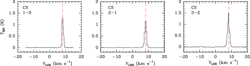
Figure 13: Observed lines of CS in B 335 (black) with rms$>$3$\sigma$. The red dashed line indicates the systemic velocity of the source v_LSR=8.3 km s^-1.

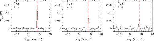
Figure 14: Observed lines of ¹³CS in B 335 (black) with rms$>$3$\sigma$. The red dashed line indicates the systemic velocity of the source v_LSR=8.3 km s^-1.

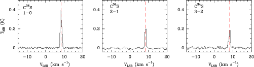
Figure 15: Observed lines of C³⁴S in B 335 (black) with rms$>$3$\sigma$. The red dashed line indicates the systemic velocity of the source v_LSR=8.3 km s^-1.

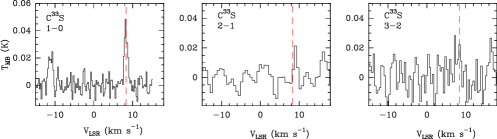
Figure 16: Observed lines of C³³S in B 335 (black) with rms$>$3$\sigma$. The red dashed line indicates the systemic velocity of the source v_LSR=8.3 km s^-1.

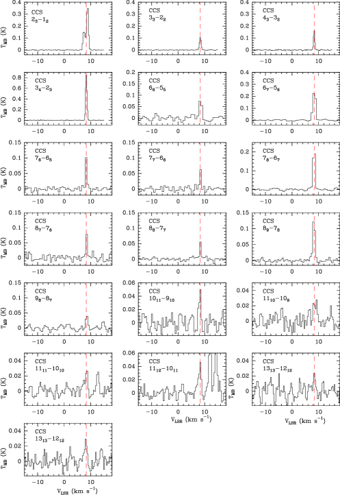
Figure 17: Observed lines of CCS in B 335 with rms$>$3$\sigma$. The red dashed line indicates the systemic velocity of the source v_LSR=8.3 km s^-1.

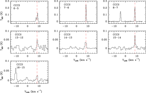
Figure 19: Observed lines of CCCS in B 335 with rms$>$3$\sigma$. The red dashed line indicates the systemic velocity of the source v_LSR=8.3 km s^-1.

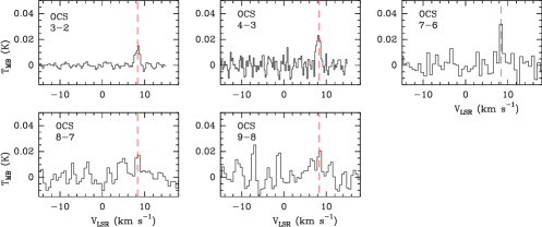
Figure 21: Observed lines of OCS in B 335 with rms$>$3$\sigma$. The red dashed line indicates the systemic velocity of the source v_LSR=8.3 km s^-1.

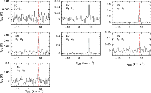
Figure 24: Observed lines of SO in B 335 with rms$>$3$\sigma$. The red dashed line indicates the systemic velocity of the source v_LSR=8.3 km s^-1.

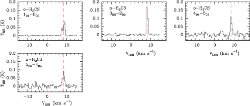
Figure 26: Observed lines of o-H₂CS in B 335 with rms$>$3$\sigma$. The red dashed line indicates the systemic velocity of the source v_LSR=8.3 km s^-1.

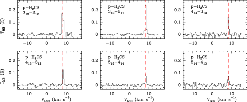
Figure 27: Observed lines of p-H₂CS in B 335 with rms$>$3$\sigma$. The red dashed line indicates the systemic velocity of the source v_LSR=8.3 km s^-1.

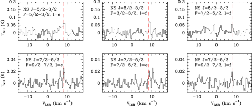
Figure 28: Observed lines of NS in B 335 with rms$>$3$\sigma$. The red dashed line indicates the systemic velocity of the source v_LSR=8.3 km s^-1.

We have detected 81 emission lines from 21 different sulphur-bearing species (including isotopologs) in B 335. In particular, we have detected three transitions of CS, three of ¹³CS, three of C³⁴S, three of C³³S, nineteen of CCS, three of CC³⁴S, seven of CCCS, three of CCC³⁴S, five of OCS, three of HCS⁺, two of HC³⁴S⁺, seven of SO, one of SO₂, one of ³⁴SO, one of H₂S, one of H₂³⁴S, ten of H₂CS, one of HSCN, one of HNCS, and six of NS (see Table LABEL:table:line_parameters and Figs. 13-33 in Appendix). These transitions span an energy range of $E_{\mathrm{up}}$=2.0-65.3 K.

4.1 Line profiles

All the lines are observed in emission. We first fitted the observed lines with Gaussian profiles using the CLASS software to derive the radial velocity (v_LSR), the line width, and the intensity for each line. Results are given in Table LABEL:table:line_parameters. We observed that most of the detected molecules show narrow line profiles ($\Delta$v$\lesssim$1.5 km s^-1) that can be adjusted by a single velocity component.

It is well known that the gravitational collapse of a molecular cloud when a new star is formed is accompanied by the development of highly supersonic outflows (e.g. Bachiller & Pérez Gutiérrez 1997; Holdship et al. 2019). The material ejected through these jets collides with the surrounding cloud, compressing and heating the gas, which leads to a drastic alteration of the chemistry as endothermic reactions become efficient and dust grains are partially destroyed. Many observations have shown that several sulphur-bearing species are enhanced in the shocked regions with respect to other areas of the cloud (e.g. Pineau des Forets et al. 1993; Bachiller & Pérez Gutiérrez 1997; Codella & Bachiller 1999; Wakelam et al. 2004, 2005; Esplugues et al. 2013). However, the sulphur lines observed in B 335 present very narrow line widths (Figs. 13-33), which is more consistent with the emission arising from the ambient quiescent cloud. Only for H₂S, formed through the hydrogenation of sticked atomic sulphur on grains (Hatchell et al. 1998; Garrod et al. 2007; Esplugues et al. 2014; Oba et al. 2019) and thought to be the main sulphur reservoir in ices (Vidal et al. 2017; Navarro-Almaida et al. 2020), it is necessary to also consider a wider component (with $\Delta$v=2.5 km s^-1) to fit its only detected line, since the line profile shows the presence of faint wings. This could indicate that part of the H₂S emission arises from the outflow, however, the line width of this component is much smaller ($\sim$2.5 km s^-1) than the ones observed for ¹²CO ($\sim$10-20 km s^-1) in the outflow (Yen et al. 2010). Therefore, the wider H₂S emission may be likely related to infall motions.

On the other hand, there are some species (CCS, CCCS, and H₂CS) whose low transition lines present a double peak emission. The peak with the lowest intensity is located for all the cases at lower velocity (v_LSR=7.39-8.1 km s^-1, blue peak) than for the more intense peak (v_LSR=8.80-8.97 km s^-1, red peak). Line widths are slightly larger ($\Delta$v$\lesssim$0.83-1.63 km s^-1) in the blue peaks than in the red ones ($\Delta$v$\lesssim$0.55-0.83 km s^-1). The comparison of these profiles with those from the less abundant isotopologues shows that these two-peak profiles are due to self-absorption due to the large optical depths. All the detected lines present 0.005$<$$T_{\mathrm{MB}}$$<$1.5 K.

4.2 Rotational diagrams

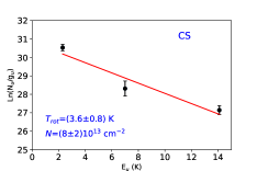
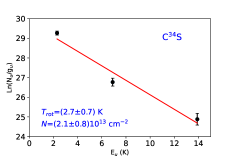
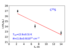
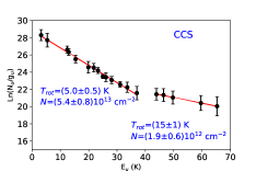
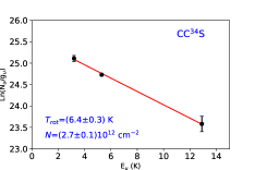
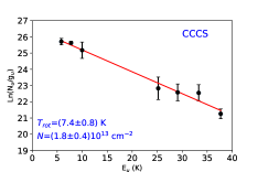
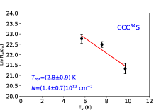
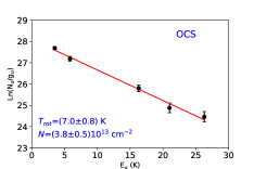
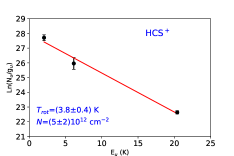
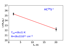
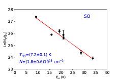
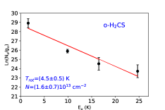
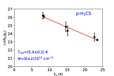
Figure 1: Rotational diagrams of the detected sulphur-bearing molecules in B 335. Fitted values of the rotational temperature, $T$_rot, column density, $N$, and their respective uncertainties are also indicated for each molecule.

For each molecule, we have computed a representative rotational temperature ($T$_rot) and a column density ($N$) by constructing a rotational diagram, assuming a single rotational temperature for all energy levels (Goldsmith & Langer 1999). Rotational diagrams represent a technique to analyse cloud properties from molecular line emission assuming local thermodynamic equilibrium (LTE). The standard relation for the rotational diagram analysis is

$$\mathrm{ln}(\frac{N_{\mathrm{u}}}{g_{\mathrm{u}}})=\mathrm{ln}N-\mathrm{ln}Z-\frac{E_{\mathrm{u}}}{kT_{\mathrm{rot}}},$$ (2)

with $N$_u/$g$_u given by

$$\frac{N_{\mathrm{u}}}{g_{\mathrm{u}}}=\frac{8k\pi}{hc^{3}}\times\frac{\nu^{2}_{\mathrm{ul}}}{A_{\mathrm{ul}}g_{\mathrm{u}}}\times{f}^{-1}\times\int T_{\mathrm{MB}}d$v$,$$ (3)

where $N$_u is the column density of the upper level in the optically thin limit, $N$ is the total column density, $g$_u is the statistical weight of the upper state of each level, $Z$ is the partition function evaluated at a rotational temperature $T$_rot, $E$_u/k is the energy of the upper level of the transition, $\nu$_ul is the frequency of the $u$→$l$ transition, $\int$ $T$_MB dv is the velocity-integrated line intensity corrected from beam efficiency, and $f$ is the beam filling factor. Assuming that the emission source has a 2D Gaussian shape, $f$ is equal to $f$_bf=$\theta$${}^{2}_{\mathrm{s}}$/($\theta$${}^{2}_{\mathrm{s}}$ + $\theta$${}^{2}_{\mathrm{b}}$) being $\theta$_b the HPBW of the telescope in arcsec and $\theta$_s the diameter of the Gaussian source in arcsec. In order to derive the values of $f$ in each case, we have used the HPBW values listed in Table 1, and we have assumed a source size of 10$\arcsec$ according to interferometric maps of C¹⁷O emission in B 335 (Cabedo et al. 2021).

The resulting rotational diagrams are shown in Fig. 1, while the column densities and rotational temperatures obtained are listed in Table LABEL:table:results_from_RD. The uncertainties shown in Table LABEL:table:results_from_RD indicate the uncertainty obtained in the least squares fit of the rotational diagrams. These uncertainties include the 10$\%$ error in the observed line intensities due to calibration. The uncertainty obtained in the determination of the line parameters with the Gaussian fitting programme is included within the error bars at each point of the rotational diagram. We did not applied the rotational diagram method to NS since its four observed lines are close to the detection limit and/or blended with other species, which would introduce a high uncertainty in the results. The analysis of NS and others molecules with only one emission line detected (e.g. SO₂) has been done only with a LVG code (see next Section) instead.

The obtained rotational temperatures are $\lesssim$15 K. In the case of CCS, the molecule with the largest number of detected transitions, we observe a trend variation (Fig. 1) between the low and the high transition energies. In particular, the transitions with $E$_u¡40 K are well adjusted for a $T$_rot$\sim$5 K, while transitions with $E$_u¿40 K are better adjusted for a $T$_rot$\sim$15 K. This suggests that CCS arises from different regions characterised by distinct excitation temperatures. The rotational temperatures for the rest of molecules with several detected transitions (e.g. C₃S, OCS, SO, H₂CS) have 4.5$\lesssim$$T$_rot$\lesssim$7.4 K. These low temperatures together with their narrow line widths are consistent with emission arising from a cold and extended part of the dense core. Gas density at these scales is probably not too high as also indicated by the low $T$_rot obtained for most of the S-molecules. All this suggests that the gas is sub-thermally excited with a moderate or low ($<$10⁵ cm^-3) density, in agreement with Frerking et al. (1987). In addition, the low number of transitions detected for several species (CS, ¹³CS, C³⁴S, C³³S, HCS⁺, and HC³⁴S⁺) and the optically thick emission of some transitions of CCS, CCCS, and H₂CS, also indicate that the rotational diagram method not suitable to derive column densities.

Table 2: Column densities ($N$), rotational temperatures, and abundances ($X$) relative to H₂ of the sulphur-bearing molecules detected in B 335.

Species	$N$rot$\times$1013	$T$rot	a$N$LVG$\times$1013	b$X$$\times$10-9
	(cm-2)	(K)	(cm-2)
CS	8$\pm$2	3.6$\pm$0.8	12.00 (34.2)	11.0
13CS	0.8$\pm$0.1	2.8$\pm$0.9	0.73	0.24
C34S	2.1$\pm$0.8	2.7$\pm$0.7	1.40	0.45
C33S	0.18$\pm$0.09	2.9$\pm$0.5	0.13	0.04
CCS	5.4$\pm$0.8	5$\pm$0.5	4.40	1.42
	0.19$\pm$0.06	15$\pm$1
CC34S	0.27$\pm$0.01	6.4$\pm$0.3	0.90	0.29
CCCS	1.8$\pm$0.4	7.4$\pm$0.8	0.65	0.02
CCC34S	0.14$\pm$0.07	2.8$\pm$0.9	0.12	0.04
OCS	3.8$\pm$0.5	7.0$\pm$0.8	2.00	0.65
HCS+	0.5$\pm$0.2	3.8$\pm$0.4	0.55 (1.5)	0.05
HC34S+	0.08$\pm$0.02	6$\pm$1	0.06	0.01
SO	1.8$\pm$0.6	7.2$\pm$0.1	6.10	1.97
34SO	-	-	0.25	0.08
o-H2CS	1.6$\pm$0.7	4.5$\pm$0.5	1.00	0.32
p-H2CS	0.6$\pm$0.2	5.4$\pm$0.2	0.70	0.22
NS	-	-	0.13	0.04
SO2	-	-	0.47	0.21
H2S	-	-	6.50	2.10
H234S	-	-	0.11	0.04
HSCN	-	-	0.10	0.03
HNCS	-	-	0.47	0.15
Total $N$			6.2$\times$1014
Total $X$				2.0$\times$10-8

Numbers in parentheses are obtained from its corresponding ³⁴S isotopologue considering ³²S/³⁴S=24.4 (Mauersberger et al. 2004).
^a LVG calculations assuming $n$${}_{\mathrm{H_{2}}}$=5$\times$10⁴ cm^-3 and $T$_K=15 K (Shirley et al. 2011; Cabedo et al. 2021).
^b Considering $N$${}_{\mathrm{H_{2}}}$=3.1$\times$10²² cm^-2 (Cabedo et al. 2021).

4.3 Column densities and abundances

We have therefore calculated molecular column densities for the detected S-species using a large velocity gradient (LVG) approximation. In particular, we have derived them by fitting the emission line profiles using the LVG code MADEX (Cernicharo 2012), which assumes that the radiative coupling between two relatively close points is negligible, and the excitation problem is local. The LVG models are based on the Goldreich & Kwan (1974) formalism. MADEX also includes corrections for the beam dilution of each line, depending on the different beam sizes at different frequencies. The final considered fit is the one that reproduces more line profiles better from all the observed transitions. To carry out the fits, we assume uniform physical conditions (kinetic temperature, density, line width, radial velocity). In particular, we have assumed a gas density of 5$\times$10⁴ cm^-3 according to results from Sect. 4.2 and to results from Cabedo et al. (2023), who deduced a density of $\sim$10⁴ cm^-3 for the outer regions of B 335 based on interferometric observations. We have also assumed a source size of 10$\arcsec$ according to interferometric maps (Cabedo et al. 2021), and a kinetic temperature of the gas $T$_K$\sim$15 K estimated by Shirley et al. (2011) from the formula for dust temperature considering only central heating by the B 335 protostar, and that dust and gas are coupled.

In the case of H₂CS and H₂S, we have used the code RADEX (van der Tak et al. 2007) since there are not available collisional rates in MADEX for these two molecules. The results are shown in Table LABEL:table:results_from_RD. For those species for which one transition is observed (³⁴SO, SO₂, H₂S, H₂³⁴S, HSCN, and HNCS), we have derived their column densities using only the LVG approximation and not the rotational diagram technique described in Section 4.2. For NS, since there are not available collisional rates, we have considered LTE approximation.

Column densities derived using the rotational diagram technique and LVG calculations agree within a factor $\lesssim$3. Sources of uncertainty are the low angular resolution of the used telescopes (with beam sizes between $\sim$36$\arcsec$ and $\sim$54$\arcsec$ for the 40m-Yebes telescope, and $\sim$14$\arcsec$ and $\sim$29$\arcsec$ for the 30m-IRAM telescope depending on frequency), which implies that the emission from the inner region of the B 335 is blended with the outer envelope, the possible overlap with the emission from other species (e.g. the case of H₂³⁴S), the limited number of detected transitions (one transition in many cases, such as for H₂S, H₂³⁴S, SO₂, HSCN, HNCS, and ³⁴SO), the lack of collisional rates for some species (e.g. NS), and the assumed source size derived from C¹⁷O interferometric observations. This is one of the most important uncertainties due to the lack of interferometric observations of S-species in B 335, since the emission from the different S-molecules may arise from distinct regions with slightly different sizes leading to a significant impact on the fits. In order to derive the uncertainty associated with the LVG results, we have run the LVG code varying the considered values for density, temperature, and source size. In particular, we have run models with density 5$\times$10⁴ cm^-3 and 2.5$\times$10⁴ cm^-3 (variation of a factor 2), temperatures of 15 K and 12 K, and source sizes of 10$\arcsec$ and 8 $\arcsec$ (reduction of 20$\%$). We found variations in the S-column densities $\lesssim$10$\%$ between these two $T$_K which is comparable to the calibration errors, while the variations when changing the density and the source size were $\lesssim$20$\%$ and $\sim$30$\%$, respectively. Taking all this into account, we estimate the uncertainties in the column densities derived with LVG approximation to be of the order of $\sim$50$\%$.

The total column density of the sulphur-bearing species observed in B 335 is 6.2$\times$10¹⁴ cm^-2, with the highest contribution coming from CS (calculated from C³⁴S considering ³²S/³⁴S=24.4 since CS is optically thick, Mauersberger et al. 2004), H₂S, SO, and CCS. The lowest values are found for NS and HSCN. We have also observed several isotopologues relative to ¹³C, ³⁴S, and ³³S. In particular, from CS, we obtain ³⁴S/³³S=10.7 (which is slightly higher than the solar abundance value ³⁴S/³³S=5.6-6.3, Anders & Grevesse 1989; Mauersberger et al. 2004), and ¹²C/¹³C=46.8, which is similar to that found in dark clouds by Cernicharo & Guelin (1987).

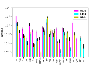
Figure 2: Comparison of fractional abundances of sulphur-bearing species between three Class 0 objects B 335 (this work), L 483 (Agúndez et al. 2019), and B1-b (Fuente et al. 2016).

Table LABEL:table:results_from_RD also shows the fractional abundances relative to H₂ (with $N$${}_{\mathrm{H_{2}}}$ obtained from Cabedo et al. 2021) of the sulphur molecules detected in the range $\lambda$ = 2, 3, and 7 mm. Considering the detected S-molecules, we have obtained a total molecular sulphur abundance of 2.0$\times$10^-8, which is alike to the one found in similar sources, such as L 1544 (1.1$\times$10^-8, Vastel et al. 2018), L 483 (9.1$\times$10^-9, Agúndez et al. 2019), and B1-b (1.2$\times$10^-8, Fuente et al. 2016). The highest S-abundances are $>$10^-9 (CS, H₂S, CCS, and SO), with also several relatively abundant ($>$10^-10) species, such as OCS and H₂CS. In general, B 335 presents a great variety of S-bearing molecules, but less than other similar sources. In particular, although the total sulphur abundance in B 335 is similar to other sources, such as L 483, we detect a significant lower number of sulphur molecules in B 335 than in L 483. We are also missing some other S-species already reported towards L 483, including SO⁺, HCS, and CH₃SH, for which we have derived upper limits for their column densities of $N$(SO⁺)$<$1.5$\times$10¹¹ cm^-2, $N$(HCS)$<$3$\times$10¹² cm^-2, and $N$(CH₃SH)$<$2$\times$10¹² cm^-2. To derive these upper limits, once the physical parameters are fixed, we vary (for each species) the column density until the model fit reaches the observed intensity peak of any of the observed lines. We do not allow the model fit to be greater than any observed line.

5 discussion

5.1 Chemical comparison

Even though the total sulphur abundance in B 335 is similar to that from other Class 0 sources, the abundances of some specific molecules significantly vary among them. Figure 2 shows a comparison between abundances of different sulphur species in three Class 0 sources, B 335, L 483, and B1-b. The first thing that stands out is that sulphur carbon chains (CS, CCS, and CCCS) in B 335 are about one order of magnitude higher than the ones observed in L 483 and B1-b. Although high abundances of carbon-chain molecules have already been found in other cold clouds, such as TMC1 (Agúndez & Wakelam 2013), it is not a universal characteristic of this type of early regions, since many of them present different degrees of carbon chain richness (e.g. Suzuki et al. 1992; Hirota et al. 2009). This therefore highlights the nature of B 335 as a source especially rich in sulphur carbon chains.

Unlike carbon chains, sulphur molecules containing oxygen in B 335 have a similar (OCS) or even lower (SO and SO₂) abundance by up to one order of magnitude than those found in L 483 and B1-b (see also Fig. 3). These oxygen-sulphur molecules are usually detected in cold dense regions with abundances between 10^-10-10^-8, while in hot cores and hot corinos they are significantly enhanced (e.g. Tercero et al. 2010; Esplugues et al. 2013). In particular, SO₂ is a better tracer of warm gas than SO (Esplugues et al. 2013), while SO is a well-known outflow tracer (e.g. Codella & Scappini 2003; Lee et al. 2010; Tafalla et al. 2010). SO seems to be more enhanced than SO₂ in shocks for timescales $\sim$10⁴ yr (e.g. Codella & Bachiller 1999; Viti et al. 2004; Jiménez-Serra et al. 2005). The low SO abundance found in B 335 with respect to the other two sources L 483 and B1-b suggests that its chemistry may not be significantly affected by shocks associated with the bipolar outflow (e.g. Hirano et al. 1988, 1992; Stutz et al. 2008; Bjerkeli et al. 2019).

Other sulphur molecules detected in B 335 with low abundances (Fig. 3) are those containing nitrogen, that is NS and HSCN (4$\times$10^-11 and 3$\times$10^-11, respectively). HSCN, unlike HNCS which is the most stable isomer, is metastable and only detected on Earth under specific conditions (through UV-photolysis of HNCS (Wierzejewska & Mielke 2001) or through a low-pressure discharge (Brünken et al. 2009)). In contrast, HSCN is more easily observed in the interstellar medium. For instance, in Sgr B2 (where HSCN was first time detected) the ratio HNCS/HSCN$\sim$3 (Halfen et al. 2009) and in TMC1 this ratio is $\sim$1 (Adande et al. 2010), while in L 1544 Vastel et al. (2018) only detect HSCN, but not HNCS. This shows the important role of non-equilibrium chemistry in dense clouds. In B 335, we only detect one transition of HNCS with a signal to noise ratio $\sigma$$\sim$3.1, so we have considered its column density ($N_{\mathrm{HNCS}}$$\leq$4.7$\times$10¹² cm^-2) as an upper limit. This leads to a ratio HNCS/HSCN$<$4.7 consistent with the one found in Sgr B2.

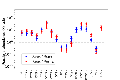
Figure 3: Fractional abundance ($X$) ratios between B 335 and L 483, and B 335 and B1-b for all the detected sulphur-bearing species in B 335.

5.2 Sulphur ions

Apart from neutral sulphur species, we have also observed the presence of some ions in B 335. Molecular ions are commonly observed in dense prestellar or protostellar regions (e.g. Caselli et al. 1998; Hogerheijde et al. 1998; Caselli et al. 2002; van der Tak et al. 2005). To a lesser extent, ions (such as HCO⁺ and N₂H⁺) have also been observed in protostellar shocks (e.g. Bachiller & Pérez Gutiérrez 1997; Hogerheijde et al. 1998; Caselli et al. 2002; van der Tak et al. 2005). The presence of ions in shocked regions is a balance between their enhancement by the sputtering of dust grain mantles, which ejects molecules into the gas phase that undergo reactions forming ions, and their destruction by electronic recombination (e.g. Neufeld & Dalgarno 1989; Viti et al. 2002). For this reason, those ions that usually decrease in shocks (such as N₂H⁺) may indicate the presence of a pre-shock chemistry (Codella et al. 2013), while the ions that are enhanced by shock chemistry will be effective tracers of shocked gas. This is the case of HOCO⁺ and SO⁺ (Podio et al. 2014) since their abundances are predicted to be very low in the quiescent gas, but significantly enhanced in shocks following the release of CO₂ and S-species from dust grain mantles (Minh et al. 1991; Turner 1992, 1994; Deguchi et al. 2006).

Among the sulphur ions, in B 335 we do not detect SO⁺ (strong tracer of shocked gas which forms from S⁺ and OH Neufeld & Dalgarno 1989), but we detect HCS⁺ and HC³⁴S⁺ with abundances of 4.7$\times$10^-10 and 1.9$\times$10^-11, respectively. The value we have obtained for HCS⁺ is similar to the one observed in the bow shock L 1157-B1 (Podio et al. 2014) and one order of magnitude higher than the ones obtained by Agúndez et al. (2019) and Fuente et al. (2016) in the Class 0 objects L 483 and B1-b, respectively, as also found for CS. The abundances of HCS⁺ and CS are strongly related, since this ion forms through the reaction of CS with HCO⁺, H${}^{+}_{3}$, H₃O⁺ (Millar et al. 1985). In addition, large abundances of CS and HCS⁺ may also indicate that OCS is one of the main sulphur carriers on dust grains upon sputtering from the grain mantles according to previous theoretical (Podio et al. 2014) and observational (Wakelam et al. 2005; Codella et al. 2005) results.

Regarding the ratio $R$=HCS⁺/CS, we obtain from observations a value of 0.043. Thaddeus et al. (1981) determined an abundance ratio $R$$\sim$0.01-0.03 in ten molecular sources located in Sgr B2 and Ori A, while Millar (1983) found that $R$ could be as large as 0.1 in cold dark clouds. This result was also verified by Irvine et al. (1983). A similar $R$ value to that from B 335 is found as well in the pre-stellar core L 1544 (0.03, Vastel et al. 2018), while in the protostellar sources L 483 and B1-b the HCS⁺/CS ratio is 0.017 and 0.008, respectively (Agúndez et al. 2019; Fuente et al. 2016). According to Clary et al. (1985), rate coefficients for ion-CS reactions rapidly increase at low temperatures suggesting that the sources B 335 and L 1544 are characterised by lower temperatures than L 483 and B1-b, which can be due to an earlier evolutionary stage of B 335 and L 1544 compared to L 483 and B1-b.

5.3 Time evolution of fractional abundances

Figures 4-7 show the evolution of several S-bearing species along 10 Myr for different physical conditions of the cosmic-ray (CR) ionisation rate ($\zeta$${}_{\mathrm{H_{2}}}$), gas temperature ($T$_g), hydrogen number density ($n$_H), and initial sulphur abundance ($S$${}^{+}_{\mathrm{init}}$). Given that the CR ionisation rate is still uncertain and spreads over a range of values (van der Tak & van Dishoeck (2000) determined as $\zeta$${}_{\mathrm{H_{2}}}$$\sim$3$\times$10^-17 s^-1 in dense clouds, Indriolo & McCall (2012) obtained a range (1.7-10.6)$\times$^-16 s^-1 in a sample of diffuse clouds, and Neufeld & Wolfire (2017) derived a $\zeta$${}_{\mathrm{H_{2}}}$ of the order of a few 10^-16 s^-1 in the Galactic disk), we have considered two values for the cosmic ionisation rate $\zeta$${}_{\mathrm{H_{2}}}$=1.3$\times$10^-16 s^-1 and 1.3$\times$10^-17 s^-1. For the gas temperature and density, given the results obtained in Sects. 4.2 and 4.3, we have run models considering $T$_g=7 K and 15 K, and $n$_H=2$\times$10⁴ cm^-3 and 2$\times$10⁵ cm^-3. For the case of the initial sulphur abundance, we have considered the solar elemental sulphur fractional abundance ($S$${}^{+}_{\mathrm{init}}$=1.5$\times$10^-5) and also one factor of S depletion (1.5$\times$10^-6) since to reproduce observations in hot corinos one needs to assume a significant sulphur depletion of at least one order of magnitude lower than the solar elemental sulphur abundance as previously stated in Sect. 1.

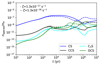
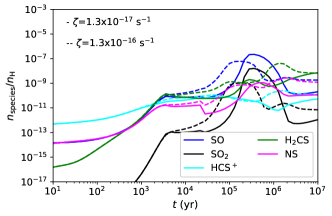
Figure 4: Evolution of fractional abundances of CS, CCS, C₃S, OCS, SO, SO₂, HCS⁺, H₂CS, and NS as a function of time for an initial sulphur abundance $S$${}^{+}_{\mathrm{init}}$=1.5$\times$10^-6, a hydrogen number density $n$_H=2$\times$10⁴ cm^-3, $T$_gas=7 K, and two values of CR ionisation rate $\zeta$=1.3$\times$10^-17 s^-1 (solid line) and $\zeta$=1.3$\times$10^-16 s^-1 (dashed line).

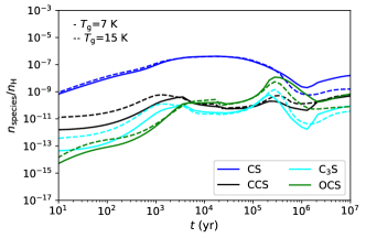
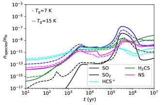
Figure 5: Evolution of fractional abundances of CS, CCS, C₃S, OCS, SO, SO₂, HCS⁺, H₂CS, and NS as a function of time for an initial sulphur abundance $S$${}^{+}_{\mathrm{init}}$=1.5$\times$10^-6, a hydrogen number density $n$_H=2$\times$10⁴ cm^-3, $T$_gas=7 K, and two values of CR ionisation rate $\zeta$=1.3$\times$10^-17 s^-1 (solid line) and $\zeta$=1.3$\times$10^-16 s^-1 (dashed line).

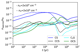
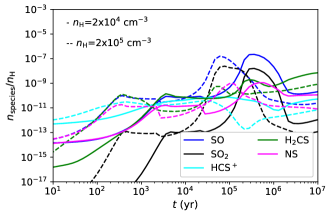
Figure 6: Evolution of fractional abundances of CS, CCS, C₃S, OCS, SO, SO₂, HCS⁺, H₂CS, and NS as a function of time for an initial sulphur abundance $S$${}^{+}_{\mathrm{init}}$=1.5$\times$10^-6, a hydrogen number density $n$_H=2$\times$10⁴ cm^-3, $T$_gas=7 K, and two values of CR ionisation rate $\zeta$=1.3$\times$10^-17 s^-1 (solid line) and $\zeta$=1.3$\times$10^-16 s^-1 (dashed line).

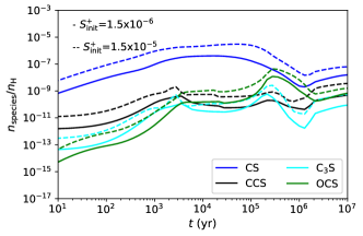
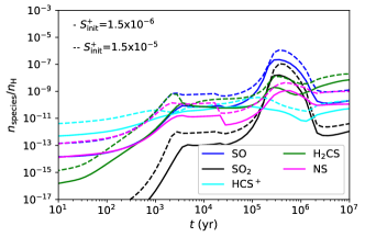
Figure 7: Evolution of fractional abundances of CS, CCS, C₃S, OCS, SO, SO₂, HCS⁺, H₂CS, and NS as a function of time for an initial sulphur abundance $S$${}^{+}_{\mathrm{init}}$=1.5$\times$10^-6, a hydrogen number density $n$_H=2$\times$10⁴ cm^-3, $T$_gas=7 K, and two values of CR ionisation rate $\zeta$=1.3$\times$10^-17 s^-1 (solid line) and $\zeta$=1.3$\times$10^-16 s^-1 (dashed line).

We have obtained these models using the Nautilus time-dependent chemical code (Ruaud et al. 2016). Nautilus is a three-phase model in which gas, surface icy mantle, bulk icy mantle, and their interactions are considered. Nautilus solves the kinetic equations for both the gas phase species and the surface species of interstellar dust grains and computes the evolution with time of chemical abundances for a given physical structure. The chemical network is based on the KInetic Database for Astrochemistry (KIDA). The used version here is detailed in Wakelam et al. (2021). In particular, this Nautilus version considers gas-phase processes including neutral-neutral and ion-neutral reactions, direct cosmic ray ionisation or dissociation, ionisation or dissociation by UV photons, ionisation or dissociation produced by photons induced by cosmic-ray interactions with the medium (Prasad & Tarafdar 1983), and electronic recombinations. For species on the surfaces, there is a distinction between species in the most external layers (surface species) and species below these layers (mantle species). The species are adsorbed on the surface and become the mantle during the construction of the ices. Similarly, when the species desorb, only the species from the surface can desorb, but surface species are gradually replaced by the mantle species. Regarding surface reactions, the model includes thermal desorption, photo-desorption, chemical desorption, and cosmic-ray heating. See Wakelam et al. (2021) for extensive details about the surface parameters considered in each surface reaction. In all models, we have adopted the initial abundances shown in Table LABEL:table:abundances_Nautilus and a visual extinction $A$_V=15 mag.

Table 3: Abundances with respect to total hydrogen nuclei considered in the chemical code Nautilus.

Species	Abundance	Reference
He	9.0$\times$10-2	(1)
O	2.4$\times$10-4	(2)
Si+	8.0$\times$10-9	(3)
Fe+	3.0$\times$10-9	(3)
S+	1.5$\times$10-5, 1.5$\times$10-6	(1)
Na+	2.0$\times$10-9	(3)
Mg+	7.0$\times$10-9	(3)
P+	2.0$\times$10-10	(3)
Cl+	1.0$\times$10-9	(3)
F+	6.7$\times$10-9	(4)
N	6.2$\times$10-5	(5)
C+	1.7$\times$10-4	(5)

In general, we observe that the abundances of all the species considered in Figs. 4-7 increase with time up to $t$$\sim$5$\times$10⁵ yr, moment at which the abundances of various species decrease abruptly. This is the case of CS, SO, and SO₂, whose abundances decrease by about 2-4 orders of magnitude between $t$$\sim$5$\times$10⁵ yr and $t$$\sim$5$\times$10⁶ yr since they react with other species to form more complex molecules. In particular, for $t$$>$10⁵ yr, CS SO, and SO₂ are mainly destroyed by reacting with H${}^{+}_{\mathrm{3}}$ and forming HCS⁺, HSO⁺, and HSO${}^{+}_{\mathrm{2}}$, respectively. For the abundances of the rest of sulphur species, this decrease after reaching the maximum value is lower and not greater than two orders of magnitude. From these figures, we also deduce the formation time scales of S-species. In particular, we have observed that CS is one of the molecules reaching first its maximum abundance value in all the models at $t$$\sim$5$\times$10⁴ yr, followed by HCS⁺ with its maximum abundance reached at $t$$\sim$10⁵ yr. Other molecules, such as H₂CS, can be considered as late molecules, since their maximum abundance values are found when the chemical evolution exceeds one million years.

Regarding the influence of the physical conditions (cosmic-ray ionisation rate, temperature, density, and initial sulphur abundance) on the S-abundances, the parameter with the highest impact is the hydrogen nuclei number density, $n$_H, since varying $n$_H by one order of magnitude leads to abundance variations of up to three orders of magnitude for CS, CCS, OCS, HCS⁺, SO, and SO₂ given a specific evolutionary time (see Fig. 6). In general terms, we observe in Fig. 6 that the chemical evolution of each considered species is accelerated when the density increases since collisions are more frequent than in a low density regime. This results in the abundance peak of the species being reached at earlier times for larger densities, although the chemical behaviour along time is roughly maintained. In particular, for $t$$\sim$10⁴ yr, we obtain that SO₂ is mainly formed by the reaction O+SO for $n$_H=2$\times$10⁴ and 2$\times$10⁵ cm^-3, while for $t$$\sim$10⁵ yr (when the SO₂ peak is reached) this molecule mainly forms by the reaction O+SO for $n$_H=2$\times$10⁴ cm^-3 and by OH+SO for $n$_H=2$\times$10⁵ cm^-3. The most responsible species of destroying SO₂ for both densities is C for $t$$\sim$10⁴ yr, and H${}^{+}_{\mathrm{3}}$ for $t$$\geq$10⁵ yr. Regarding CS, for $t$$\sim$10⁴ yr, it is mainly formed by the reaction HCS⁺+e^- for the low density value, while CS is mainly formed through the reaction between atomic S and C₄ for $n$_H=2$\times$10⁵ cm^-3. For $t$$\sim$10⁵ yr (when the CS abundance decreases for any model), CS is mainly destroyed by its reaction with H${}^{+}_{\mathrm{3}}$ and with HCO⁺.

Another parameter with a big impact on S-abundances is the cosmic-ray ionisation rate, $\zeta$, since the variation from $\zeta$=1.3$\times$10^-17 to 1.3$\times$10^-16 s^-1 changes by about two orders of magnitude the abundances of all the sulphur species considered in the sample (Fig. 4). For the case of carbon-chains (CCS, C₃S), we observe that the larger $\zeta$, the larger the S-abundances for $t$$\lesssim$10⁵ yr. Similar results are found for the species SO, SO₂, NS, H₂CS, and OCS. For $t$$\sim$10⁴ yr, we find that CCS is mainly formed by C+HCS for the low $\zeta$ model, while it is mainly formed through HC₃S⁺+e^- in a more efficient way for a model with larger $\zeta$ (1.3$\times$10^-16 s^-1). In the case of SO (one of the most affected molecules by $\zeta$ between 10⁴$\lesssim$$t$$\lesssim$10⁶ yr), it is mostly formed by the reaction O+HS in a model with low $\zeta$, while the reaction between S+OH becomes more important to form SO₂ when increasing $\zeta$ by one order of magnitude.

On the other hand, changing the temperature (from $T$_gas=7 K to 15 K) and especially the initial sulphur abundance (from $S$${}^{+}_{\mathrm{init}}$=1.5$\times$10^-5 to 1.5$\times$10^-6) in the models leads to abundance variations smaller than two orders of magnitude for $t$$>$10⁴ yr. In particular, we have found that an increase of the $S$${}^{+}_{\mathrm{init}}$ value by one order of magnitude also enhances the S-abundances by one order of magnitude during the entire duration of core evolution.

For the particular case of HCS⁺ and CS, the main physical parameters significantly influencing their abundances are the density (the lower density, the higher the HCS⁺ and CS abundances for $t$$>$10⁴ yr) and the cosmic-ray ionisation rate (the higher the $\zeta$, the higher the HCS⁺ and CS abundances for $t$$>$5$\times$10⁵ yr). By contrast, other physical parameters, such as the gas temperature, barely affect the HCS⁺ and CS abundances for $t$$<$10⁶ yr.

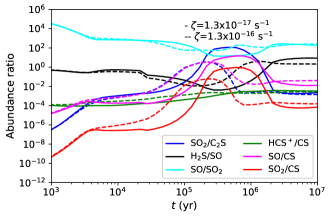
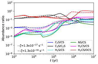
Figure 8: Evolution of fractional abundances of CS, CCS, C₃S, OCS, SO, SO₂, HCS⁺, H₂CS, and NS as a function of time for an initial sulphur abundance $S$${}^{+}_{\mathrm{init}}$=1.5$\times$10^-6, a hydrogen number density $n$_H=2$\times$10⁴ cm^-3, $T$_gas=7 K, and two values of CR ionisation rate $\zeta$=1.3$\times$10^-17 s^-1 (solid line) and $\zeta$=1.3$\times$10^-16 s^-1 (dashed line).

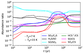
Figure 9: Evolution of fractional abundances of CS, CCS, C₃S, OCS, SO, SO₂, HCS⁺, H₂CS, and NS as a function of time for an initial sulphur abundance $S$${}^{+}_{\mathrm{init}}$=1.5$\times$10^-6, a hydrogen number density $n$_H=2$\times$10⁴ cm^-3, $T$_gas=7 K, and two values of CR ionisation rate $\zeta$=1.3$\times$10^-17 s^-1 (solid line) and $\zeta$=1.3$\times$10^-16 s^-1 (dashed line).

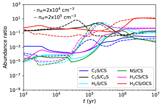
Figure 10: Evolution of fractional abundances of CS, CCS, C₃S, OCS, SO, SO₂, HCS⁺, H₂CS, and NS as a function of time for an initial sulphur abundance $S$${}^{+}_{\mathrm{init}}$=1.5$\times$10^-6, a hydrogen number density $n$_H=2$\times$10⁴ cm^-3, $T$_gas=7 K, and two values of CR ionisation rate $\zeta$=1.3$\times$10^-17 s^-1 (solid line) and $\zeta$=1.3$\times$10^-16 s^-1 (dashed line).

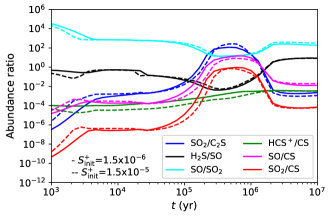
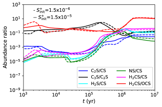
Figure 11: Evolution of fractional abundances of CS, CCS, C₃S, OCS, SO, SO₂, HCS⁺, H₂CS, and NS as a function of time for an initial sulphur abundance $S$${}^{+}_{\mathrm{init}}$=1.5$\times$10^-6, a hydrogen number density $n$_H=2$\times$10⁴ cm^-3, $T$_gas=7 K, and two values of CR ionisation rate $\zeta$=1.3$\times$10^-17 s^-1 (solid line) and $\zeta$=1.3$\times$10^-16 s^-1 (dashed line).

5.4 Comparison with observations

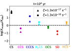
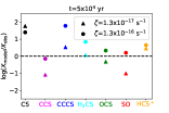
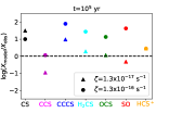
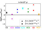
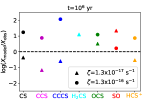
Figure 34: Ratios between the abundances obtained from the models, $X$_model, and the observations, $X$_obs, for different sulphur species at specific evolution times ($t$=10⁴, 5$\times$10⁴, 10⁵, 5$\times$10⁵, and 10⁶ yr), when varying the cosmic-ray rate ($\zeta$).

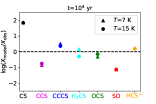
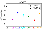
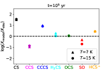
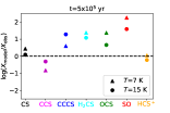
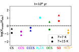
Figure 35: Ratios between the abundances obtained from the models, $X$_model, and the observations, $X$_obs, for different sulphur species at specific evolution times ($t$=10⁴, 5$\times$10⁴, 10⁵, 5$\times$10⁵, and 10⁶ yr), when varying the gas temperature.

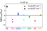
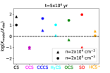
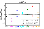
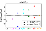
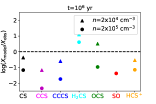
Figure 36: Ratios between the abundances obtained from the models, $X$_model, and the observations, $X$_obs, for different sulphur species at specific evolution times ($t$=10⁴, 5$\times$10⁴, 10⁵, 5$\times$10⁵, and 10⁶ yr), when varying the hydrogen number density ($n$_H).

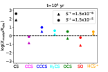
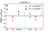
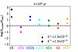
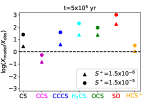
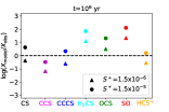
Figure 37: Ratios between the abundances obtained from the models, $X$_model, and the observations, $X$_obs, for different sulphur species at specific evolution times ($t$=10⁴, 5$\times$10⁴, 10⁵, 5$\times$10⁵, and 10⁶ yr), when varying the initial sulphur abundance ($S$${}^{+}_{\mathrm{init}}$).

We now compare the different models considered in the previous section with observational results to derive the current evolutionary stage of B335. Figures 34-37 show the ratio between the abundances obtained from the models ($X$_model) and from the observations ($X$_obs) for several sulphur-bearing species. In particular, we have considered those S-species for which we observe more than one emission line and those that are not close to the limit of detection. The results are shown for five specific evolution times ($t$=10⁴, 5$\times$10⁴, 10⁵, 5$\times$10⁵, and 10⁶ yr). In order to find the cases with the closest values between the theoretical and observational results, we have considered for each model the largest number of S-species for which -0.5$\leq$log($X$_model/$X$_obs)$\leq$0.5 in order to only consider discrepancies between model and observational results smaller than a factor of $\sim$3. Results show that the evolutionary stages that better reproduce the observed abundances of the largest number of S-species in B 335 are those between $t$=10⁴-10⁵ yr. This result obtained from a chemical approach agrees with the results obtained from Evans et al. (2015) who derived an age of $\sim$5$\times$10⁴ yr for B 335 through a dynamical perspective, by applying an inside-out collapse model that is compared with ALMA observations. Altogether this reveals, therefore, the particularly early evolutionary stage of B 335, which is comparable to the ages of pre-stellar condensations (e.g. Caselli & Ceccarelli 2012). As B 335 is an isolated globule, this may be due to the fact that the condensation has formed from very little dense gas ($\sim$10³ cm^-3) without a dense pre-phase between the formation of the globule and the beginning of the collapse. This gives B 335 a different chemistry compared to other young protostars that have form in dense molecular clouds, such as L 483 and B1-b. Another plausible scenario is that material from the diffuse cloud surrounding B 335 may currently be accreting onto the protostellar envelope, thus rejuvinating its chemistry. This accretion has been found (e.g. Pineda et al. 2020) in another Class 0 source embedded in the Perseus Molecular Cloud Complex. Interferometric observations are requested to distinguish between both scenarios.

From Figs. 34-37, we have also deduced that chemical models with values of $n$_H=2$\times$10⁴ cm^-3, $T$_g=15 K, $S$${}^{+}_{\mathrm{init}}$=1.5$\times$10^-6, and $\zeta$=1.3$\times$10^-17 s^-1 best reproduce the observations of the largest number of S-species for $t$=10⁴-10⁵ yr. This value of $\zeta$ agrees with results from Cabedo et al. (2023) who found a cosmic-ray ionisation rate $\lesssim$10^-16 s^-1 in the outer regions of B 335, especially for an envelope radii$>$500 au. A sulphur depletion factor of 10 with respect to the sulphur cosmic elemental abundance is also consistent with results from Fuente et al. (2023) in low-mass star-forming regions, such as Taurus and Perseus.

5.5 Sulphur chemical ratios

We have considered several sulphur-bearing molecular ratios and have also analysed their evolution with time. Model results obtained with the Nautilus code are shown in Figures 8-11. We have also changed some of the physical conditions (cosmic-ray ionisation rate, temperature, density, and initial sulphur abundance) in order to study their impact on the evolution of these ratios. We first notice that while there are some ratios, such as HCS⁺/CS, that present small variations of up 1 order of magnitude between $t$=10⁴-10⁶ yr, there are other ratios that significantly change with time. In particular, the SO₂/C₂S, SO/CS, SO₂/CS, NS/CS, H₂S/CS, and H₂CS/CS ratios show variations of up to $\sim$5 orders of magnitude in that time range (10⁴-10⁶ yr). The physical parameter affecting sulphur ratios the most is the density, leading to differences of up to $\sim$4-5 orders of magnitude especially between 5$\times$10⁴ and 10⁶ yr. The cosmic-ray ionisation rate is the next physical parameter with the greatest effect on the sulphur ratios with differences of about one order of magnitude in their values. In particular, the SO₂/CS, SO/CS, SO₂/C₂S, and C₂S/CS ratios are among those mostly influenced by $\zeta$, while the SO/SO₂ ratio is one of the least affected. The SO/SO₂ ratio is, however, more sensitive to the density variation. We also observe a large density impact on the NS/CS ratio, finding that the higher the density, the larger the NS/CS for $t$$\sim$10⁵-10⁶ yr, with NS being mostly formed during that time range through the neutral-neutral reaction N+HS and, to a lesser extent, through the dissociative recombination of HNS⁺. On the other hand, varying the gas temperature from 7 to 15 K (Fig. 9) mostly affects the H₂S/SO ratio between 10⁴ and 10⁶ yr, and the SO/CS, SO₂/CS, and H₂S/CS ratios at late times ($t$$\gtrsim$10⁶ yr). Regarding the only ion detected in B 335, its HCS⁺/CS ratio slightly increases when the initial sulphur abundance is decreased, and also when the cosmic-ray ionisation rate or the density increase.

The use of molecular ratios as indicators of chemical evolution of young stellar sources has been previously approached from both observational and theoretical perspectives (e.g. Pineau des Forets et al. 1993; Charnley 1997; Hatchell et al. 1998; Codella & Bachiller 1999; Gibb et al. 2000; Boogert et al. 2000; Wakelam et al. 2004). Our models (Figs. 4-7) show that SO and SO₂ constantly increase with time reaching both their peaks at $t$$\gtrsim$5$\times$10⁵ yr, which prevents the use of their ratio as a chemical clock. Nevertheless, Figures 8-11 show that there are other sulphur ratios that could be used as evolutionary tracers since they maintain a constant trend over time. This is for instance the case of the SO₂/C₂S and SO/CS ratios, whose values constantly increase during the first $\sim$2$\times$10⁵ yr. In order to compare these theoretical results with observations, we have considered a sample of sources that includes starless cores (TMC1 and L 1544 considered as starless and prestellar cores, respectively, see for example Crapsi et al. 2005; Schnee et al. 2007; Lefloch et al. 2018; Agúndez et al. 2019; Cernicharo et al. 2021) and Class 0 objects (B 335, L 483, and B1-b). Observational results are shown in Fig. 12, where we have indeed found a clear trend where the SO₂/C₂S and SO/CS ratios increase with the age of the objects, suggesting that these sulphur ratios could be used as chemical clocks. We have also included in Fig. 12 observational results for the HCS⁺/CS ratio. In this case, we have obtained a negative trend in which the value of HCS⁺/CS decreases with the age of the objects.

Comparing the observational HCS⁺/CS, SO₂/C₂S, and CO/CS ratios for B 335 with the theoretical results (Figs. 8-11), we observe that, for the temperature and density values used in Sect. 4.3 to derive observational results, the three ratios would be reproduced at 5$\times$10⁴$\lesssim$$t$$\lesssim$10⁵ yr when considering a high cosmic-ray ionisation rate ($\zeta$=1.3$\times$10^-16 s^-1) and a S depletion of at least a factor 10 with respect to the solar elemental sulphur abundance. This depletion is also found by many authors (e.g. Wakelam et al. 2004; Crockett et al. 2014; Vastel et al. 2018; Bulut et al. 2021; Navarro-Almaida et al. 2021; Esplugues et al. 2022; Hily-Blant et al. 2022; Fuente et al. 2023) in other star-forming regions.

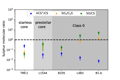
Figure 12: Observational sulphur molecular ratios of potentially good chemical evolution tracers of the prestellar to protostellar transition for different objects (TMC1, L 1544, B 335, L 483, and B1-b). Data for TMC1 were taken from Marcelino et al. (2007), Cernicharo (2012), Cernicharo et al. (2021), and Rodríguez-Baras et al. (2021). Data for L 1544 were taken from Vastel et al. (2018). L 483 and B1-b data were gathered from Agúndez et al. (2019) and Fuente et al. (2016), respectively.

6 Summary and conclusions

We have carried out a comprehensive observational and theoretical study of sulphur in the Class 0 object B 335. This source is an isolated dense Bok globule located at a distance of $\sim$100 pc. We have detected 20 different sulphur-bearing species (including isotopologues) using Yebes 40m and IRAM 30m telescope observations. In order to derive column densities, we have applied the method of rotational diagrams. For this purpose, we have also used non-LTE radiative transfer codes given the low number of transitions detected for some species and the optically thick emission of some lines. Our results show low rotational temperatures ($\lesssim$15 K), suggesting that the gas is sub-thermally excited, and thus revealing a relatively low ($<$10⁵ cm^-3) gas density. These low temperatures, the narrow line widths, and the relatively low density are also consistent with emission arising from a cold and extended region, suggesting that the detected S-emission does not trace the hot corino, but its cold envelope.

From the column densities of all the observed sulphur species, we have derived a total molecular sulphur abundance of 2.0$\times$10^-8, which is similar to that found in the envelopes of other Class 0 objects. Nevertheless, we have also found that the abundances of some specific S-molecules vary significantly across the sample of Class 0 objects (B 335, L 483, and B1-b) considered in this paper. In particular, we have derived high abundances of sulphur carbon-chain molecules in B 335 compared to those found in other Class 0 objects, and also compared with those abundances of S-molecules containing oxygen or nitrogen. This points out the nature of B 335 as a source especially rich in sulphur carbon chains, which could be due to the fact that B 335 is an isolated source compared to other young protostars that have formed in dense molecular clouds, such as L 483 and B1-b, or to accretion of material from the diffuse cloud surrounding B 335 onto the protostellar envelope, thus rejuvenating its chemistry. The comparison between envelopes of different Class 0 objects has also allowed to deduce a low SO abundance in B 335 with respect to L 483 and B1-b. SO is a well-known outflow tracer, which is thought to be enhanced in shocks. Its low abundance in B 335 together with the non-detection of other shock tracers, such SO⁺, suggests that its chemistry in B 335 is not particularly influenced by shocks.

In this work, we have also used the time-dependent chemical code Nautilus to study the time evolution of fractional S-abundances, as well as the influence of several physical and chemical parameters (cosmic-ray ionisation rate, density, gas temperature, and initial sulphur abundance) on these abundances. The comparison between chemical model results and observations shows that the evolutionary stages that better reproduce the observed abundances of the largest number of S-species in B 335 correspond to $t$=10⁴-10⁵ yr, in agreement with previous age estimations obtained by applying theoretical methods with the use of a dynamical model. The results from Nautilus have also revealed that the physical parameters with the highest influence on the S-abundances are the density and the cosmic-ray ionisation rate whose variations by one order of magnitude lead to abundance variations of several orders of magnitude for different sulphur-bearing species such as SO, SO₂, CS, and CCCS. We have also used Nautilus to explore the behaviour of different S-molecular ratios with time, finding that there are some sulphur ratios that could be used as chemical evolution tracers since they maintain a constant trend over time. A comparison of the observational results of S-ratios in a sample of objects (including starless and prestellar cores, and Class 0 objects) characterised by different evolutionary stages confirms a clear trend where the SO₂/C₂S and SO/CS ratios increase with the age of the objects, while HCS⁺/CS decreases with the evolutionary stage. We, therefore, conclude that these S-ratios could be used as good chemical evolutionary indicators tracing the prestellar to protostellar transition.

Appendix A Tables and figures

Table 4: Line parameters of sulphur-bearing molecules detected in B 335.

Species	Transition	Frequency	vLSR	$\Delta$v	$T$MB	$\int$$T$MB dv
		(MHz)	(km s-1)	(km s-1)	(K)	(K km s-1)
CS	1-0	48990.98	8.27$\pm$0.07	1.20$\pm$0.08	1.29$\pm$0.50	1.64$\pm$0.03
	2-1	97980.95	8.25$\pm$0.08	1.41$\pm$0.05	1.13$\pm$0.32	1.70$\pm$0.07
	3-2	146969.02	8.01$\pm$0.06	1.05$\pm$0.03	1.50$\pm$0.17	1.68$\pm$0.04
13CS	1-0	46247.56	8.31$\pm$0.08	0.81$\pm$0.02	0.15$\pm$0.03	0.128$\pm$0.002
	2-1	92494.27	8.34$\pm$0.04	1.34$\pm$0.07	0.06$\pm$0.01	0.095$\pm$0.007
	3-2	138739.26	8.24$\pm$0.06	0.99$\pm$0.07	0.06$\pm$0.01	0.066$\pm$0.008
C34S	1-0	48206.97	8.43$\pm$0.02	0.97$\pm$0.06	0.39$\pm$0.05	0.403$\pm$0.004
	2-1	96412.95	8.31$\pm$0.07	1.27$\pm$0.09	0.21$\pm$0.05	0.279$\pm$0.006
	3-2	144617.10	8.28$\pm$0.07	0.84$\pm$0.08	0.18$\pm$0.06	0.165$\pm$0.005
C33S	1-0	48585.88	8.17$\pm$0.05	0.80$\pm$0.08	0.04$\pm$0.01	0.041$\pm$0.004
	2-1	97172.06	9.07$\pm$0.04	0.86$\pm$0.05	0.02$\pm$0.01	0.020$\pm$0.006
	3-2	145755.62	8.21$\pm$0.07	0.80$\pm$0.06	0.02$\pm$0.01	0.020$\pm$0.007
CCS	23-12	33751.37	8.80$\pm$0.03	0.83$\pm$0.04	0.34$\pm$0.05	0.306$\pm$0.001
			7.39$\pm$0.03	1.10$\pm$0.05	0.15$\pm$0.02	0.185$\pm$0.001
	33-22	38866.42	8.29$\pm$0.05	0.77$\pm$0.04	0.11$\pm$0.02	0.087$\pm$0.001
	43-32	43981.02	8.39$\pm$0.08	0.55$\pm$0.08	0.16$\pm$0.03	0.095$\pm$0.001
	34-23	45379.03	8.35$\pm$0.02	0.67$\pm$0.06	0.85$\pm$0.07	0.606$\pm$0.001
	66-55	77731.71	8.13$\pm$0.04	1.24$\pm$0.07	0.08$\pm$0.02	0.100$\pm$0.010
	67-56	81505.17	8.05$\pm$0.01	1.52$\pm$0.07	0.22$\pm$0.03	0.357$\pm$0.006
	76- 65	86181.39	8.18$\pm$0.07	0.78$\pm$0.05	0.10$\pm$0.04	0.084$\pm$0.004
	77- 66	90686.38	8.47$\pm$0.07	0.77$\pm$0.09	0.06$\pm$0.01	0.051$\pm$0.006
	78- 67	93870.09	9.14$\pm$0.06	1.35$\pm$0.04	0.19$\pm$0.02	0.274$\pm$0.005
	87- 76	99866.52	8.54$\pm$0.03	0.75$\pm$0.03	0.08$\pm$0.02	0.061$\pm$0.007
	88- 77	103640.75	8.42$\pm$0.05	0.76$\pm$0.04	0.05$\pm$0.01	0.044$\pm$0.004
	89- 78	106347.72	7.99$\pm$0.09	1.10$\pm$0.05	0.12$\pm$0.04	0.140$\pm$0.004
	98- 87	113410.18	8.63$\pm$0.04	0.93$\pm$0.07	0.04$\pm$0.01	0.040$\pm$0.006
	1011-910	131551.96	8.38$\pm$0.03	0.72$\pm$0.04	0.05$\pm$0.01	0.038$\pm$0.007
	1110-109	140180.74	8.60$\pm$0.04	1.10$\pm$0.08	0.03$\pm$0.01	0.033$\pm$0.007
	1111-1010	142501.69	8.55$\pm$0.06	0.95$\pm$0.04	0.03$\pm$0.01	0.027$\pm$0.006
	1112-1011	144244.82	8.35$\pm$0.05	0.92$\pm$0.07	0.05$\pm$0.01	0.040$\pm$0.020
	1314-1213	169753.46	8.14$\pm$0.07	0.84$\pm$0.08	0.03$\pm$0.01	0.027$\pm$0.005
	1313-1212	168406.79	8.38$\pm$0.05	0.62$\pm$0.08	0.03$\pm$0.01	0.017$\pm$0.004
CC34S	23-12	33111.83	8.97$\pm$0.05	0.55$\pm$0.06	0.010$\pm$0.001	0.070$\pm$0.003
			8.10$\pm$0.02	1.63$\pm$0.05	0.008$\pm$0.001	0.013$\pm$0.003
	43-32	42918.18	8.37$\pm$0.04	0.60$\pm$0.05	0.008$\pm$0.001	0.030$\pm$0.002
	34-23	44497.59	8.23$\pm$0.01	0.60$\pm$0.07	0.05$\pm$0.01	0.005$\pm$0.001
CCCS	6-5	34684.36	8.78$\pm$0.03	0.66$\pm$0.08	0.12$\pm$0.02	0.090$\pm$0.001
			7.54$\pm$0.05	0.83$\pm$0.09	0.06$\pm$0.01	0.053$\pm$0.001
	7-6	40465.01	8.32$\pm$0.04	0.60$\pm$0.05	0.24$\pm$0.04	0.158$\pm$0.001
	8-7	46245.62	8.34$\pm$0.02	0.77$\pm$0.05	0.20$\pm$0.05	0.170$\pm$0.012
	13-12	75147.92	8.60$\pm$0.02	1.20$\pm$0.06	0.04$\pm$0.01	0.063$\pm$0.012
	14-13	80928.18	7.82$\pm$0.09	1.66$\pm$0.09	0.03$\pm$0.01	0.060$\pm$0.007
	15-14	86708.37	8.30$\pm$0.06	0.90$\pm$0.03	0.07$\pm$0.01	0.071$\pm$0.005
	16-15	92488.49	8.57$\pm$0.05	1.01$\pm$0.08	0.02$\pm$0.01	0.027$\pm$0.009
CCC34S	6-5	33844.24	8.77$\pm$0.04	0.84$\pm$0.05	0.005$\pm$0.001	0.005$\pm$0.001
	7-6	39484.87	8.36$\pm$0.03	0.55$\pm$0.05	0.012$\pm$0.03	0.007$\pm$0.001
	8-7	45125.47	8.33$\pm$0.04	0.41$\pm$0.07	0.009$\pm$0.003	0.004$\pm$0.001
OCS	3-2	36488.81	8.45$\pm$0.06	0.94$\pm$0.06	0.015$\pm$0.002	0.015$\pm$0.005
	4-3	48651.60	8.11$\pm$0.07	1.10$\pm$0.08	0.023$\pm$0.002	0.027$\pm$0.001
	7-6	85139.10	8.50$\pm$0.03	0.90$\pm$0.06	0.033$\pm$0.003	0.031$\pm$0.012
	8-7	97301.20	8.40$\pm$0.04	1.45$\pm$0.09	0.017$\pm$0.002	0.026$\pm$0.012
	9-8	109463.06	8.62$\pm$0.03	1.09$\pm$0.05	0.020$\pm$0.002	0.024$\pm$0.007
HCS+	1-0	42674.19	8.34$\pm$0.05	0.56$\pm$0.05	0.10$\pm$0.02	0.061$\pm$0.001
	2-1	85347.87	8.25$\pm$0.03	0.75$\pm$0.07	0.11$\pm$0.04	0.089$\pm$0.004
	4-3	170691.64	8.27$\pm$0.06	0.56$\pm$0.04	0.05$\pm$0.01	0.035$\pm$0.004
HC34S+	1-0	41983.06	8.43$\pm$0.07	0.60$\pm$0.04	0.006$\pm$0.001	0.004$\pm$0.001
	4-3	167927.26	8.90$\pm$0.08	0.75$\pm$0.08	0.023$\pm$0.01	0.018$\pm$0.006
SO	23-22	36202.04	8.77$\pm$0.09	0.51$\pm$0.05	0.005$\pm$0.001	0.003$\pm$0.001
	22-11	86093.98	8.55$\pm$0.06	0.86$\pm$0.04	0.04$\pm$0.01	0.045$\pm$0.007
	32-21	99299.90	8.35$\pm$0.07	0.91$\pm$0.07	0.56$\pm$0.04	0.550$\pm$0.006
	23-12	109252.21	8.39$\pm$0.02	1.08$\pm$0.08	0.05$\pm$0.01	0.057$\pm$0.005
	43-32	138178.68	8.32$\pm$0.02	0.81$\pm$0.06	0.37$\pm$0.02	0.318$\pm$0.006
	34-23	158971.85	8.65$\pm$0.01	0.88$\pm$0.05	0.07$\pm$0.01	0.066$\pm$0.012
	44-33	172181.40	8.38$\pm$0.05	1.00$\pm$0.08	0.06$\pm$0.01	0.071$\pm$0.009
34SO	23-12	97715.40	8.24$\pm$0.04	1.20$\pm$0.09	0.02$\pm$0.01	0.023$\pm$0.006
SO2	31,3-20,2	104029.41	8.63$\pm$0.03	1.15$\pm$0.07	0.02$\pm$0.01	0.028$\pm$0.005
H2S	11,0-10,1	168762.76	8.10$\pm$0.04	1.00$\pm$0.06	0.17$\pm$0.04	0.184$\pm$0.009
			8.30$\pm$0.03	2.50$\pm$0.10	0.11$\pm$0.03	0.290$\pm$0.008
H234S	11,0-10,1	167910.51	8.20$\pm$0.02	1.00$\pm$0.08	0.05$\pm$0.01	0.049$\pm$0.004
o-H2CS	10,1-00,0	34351.45	8.84$\pm$0.01	0.76$\pm$0.05	0.09$\pm$0.01	0.069$\pm$0.001
			7.62$\pm$0.08	0.86$\pm$0.05	0.05$\pm$0.01	0.0423$\pm$0.001
	30,3-20,2	103040.54	8.31$\pm$0.01	0.85$\pm$0.06	0.17$\pm$0.04	0.151$\pm$0.003
	40,4-30,3	137371.29	8.52$\pm$0.02	0.81$\pm$0.03	0.11$\pm$0.04	0.095$\pm$0.007
	50,5-40,4	171687.90	8.01$\pm$0.01	0.92$\pm$0.07	0.09$\pm$0.01	0.089$\pm$0.006
p-H2CS	31,3-21,2	101477.88	8.31$\pm$0.02	0.97$\pm$0.08	0.18$\pm$0.05	0.181$\pm$0.008
	31,2-21,1	104617.11	8.48$\pm$0.03	0.68$\pm$0.08	0.23$\pm$0.07	0.171$\pm$0.003
	41,4-31,3	135298.36	8.50$\pm$0.06	0.75$\pm$0.05	0.14$\pm$0.04	0.115$\pm$0.007
	41,3-31,2	139483.69	8.38$\pm$0.04	0.60$\pm$0.07	0.13$\pm$0.04	0.080$\pm$0.005
	51,5-41,4	169114.16	8.41$\pm$0.03	0.76$\pm$0.04	0.09$\pm$0.01	0.075$\pm$0.004
	51,4-41,3	174345.22	8.35$\pm$0.05	0.72$\pm$0.04	0.07$\pm$0.01	0.055$\pm$0.006
HSCN	40,4-30,3	45877.81	8.05$\pm$0.07	0.55$\pm$0.04	0.014$\pm$0.001	0.008$\pm$0.002
HNCS	30,3-20,2	35187.11	8.40$\pm$0.06	0.60$\pm$0.05	0.005$\pm$0.001	0.003$\pm$0.001
NS	$J$=5/2-3/2, $\Omega$=1/2, $F$=5/2-3/2, $l$=$e$	115156.81	8.40$\pm$0.03	1.50$\pm$0.08	0.06$\pm$0.01	0.10$\pm$0.02
	$J$=5/2-3/2, $\Omega$=1/2, $F$=3/2-3/2, $l$=$f$	115524.60	8.75$\pm$0.05	0.95$\pm$0.06	0.08$\pm$0.01	0.08$\pm$0.02
	$J$=5/2-3/2, $\Omega$=1/2, $F$=7/2-5/2, $l$=$f$	115556.25	7.95$\pm$0.06	0.90$\pm$0.06	0.06$\pm$0.01	0.05$\pm$0.02
	$J$=7/2-5/2, $\Omega$=1/2, $F$=9/2-7/2, $l$=$e$	161297.24	8.26$\pm$0.01	0.73$\pm$0.05	0.03$\pm$0.01	0.020$\pm$0.004
	$J$=7/2-5/2, $\Omega$=1/2, $F$=7/2-5/2, $l$=$e$	161298.41	8.62$\pm$0.01	0.70$\pm$0.06	0.02$\pm$0.01	0.016$\pm$0.004
	$J$=7/2-5/2, $\Omega$=1/2, $F$=9/2-7/2, $l$=$f$	161697.25	7.95$\pm$0.03	0.65$\pm$0.07	0.02$\pm$0.01	0.014$\pm$0.004

Table 4: continued.

Figure 18: Observed lines of CC³⁴S in B 335 with rms$>$3$\sigma$. The red dashed line indicates the systemic velocity of the source v_LSR=8.3 km s^-1.

Figure 20: Observed lines of CCC³⁴S in B 335 with rms$>$3$\sigma$. The red dashed line indicates the systemic velocity of the source v_LSR=8.3 km s^-1.

Figure 22: Observed lines of HCS⁺ in B 335 with rms$>$3$\sigma$. The red dashed line indicates the systemic velocity of the source v_LSR=8.3 km s^-1.

Figure 23: Observed lines of HC³⁴S⁺ in B 335 with rms$>$3$\sigma$. The red dashed line indicates the systemic velocity of the source v_LSR=8.3 km s^-1.

Figure 25: Observed lines of ³⁴SO in B 335 with rms$>$3$\sigma$. The red dashed line indicates the systemic velocity of the source v_LSR=8.3 km s^-1.

Figure 29: Observed line of SO₂ in B 335 with rms$>$3$\sigma$. The red dashed line indicates the systemic velocity of the source v_LSR=8.3 km s^-1.

Figure 30: Observed line of H₂S in B 335 with rms$>$3$\sigma$. The red dashed line indicates the systemic velocity of the source v_LSR=8.3 km s^-1.

Figure 31: Observed line of H₂³⁴S in B 335 with rms$>$3$\sigma$. The red dashed line indicates the systemic velocity of the source v_LSR=8.3 km s^-1.

Figure 32: Observed line of HSCN in B 335 with rms$>$3$\sigma$. The red dashed line indicates the systemic velocity of the source v_LSR=8.3 km s^-1.

Figure 33: Observed line of HNCS in B 335 with rms$>$3$\sigma$. The red dashed line indicates the systemic velocity of the source v_LSR=8.3 km s^-1.