On the Robustness of Post-hoc GNN Explainers to Label Noise
Abstract
Proposed as a solution to the inherent black-box limitations of graph neural networks (GNNs), post-hoc GNN explainers aim to provide precise and insightful explanations of the behaviours exhibited by trained GNNs. Despite their recent notable advancements in academic and industrial contexts, the robustness of post-hoc GNN explainers remains unexplored when confronted with label noise. To bridge this gap, we conduct a systematic empirical investigation to evaluate the efficacy of diverse post-hoc GNN explainers under varying degrees of label noise. Our results reveal several key insights: Firstly, post-hoc GNN explainers are susceptible to label perturbations. Secondly, even minor levels of label noise, inconsequential to GNN performance, harm the quality of generated explanations substantially. Lastly, we engage in a discourse regarding the progressive recovery of explanation effectiveness with escalating noise levels.
1 Introduction
The emergence of Graph Neural Networks (GNNs) has revolutionised machine learning on graph-structured data [1, 2, 3]. Nevertheless, a substantial concern has been raised within the community: GNN models can be easily manipulated/attacked [4, 5] by unnoticeable modifications. To counter this, researchers proposed robust GNN models against diverse adversarial attacks [6, 7]. However, a significant gap persists as current GNNs struggle to provide insightful interpretations of their underlying mechanisms and outputs. To tackle this limitation, recent researchers proposed post-hoc GNN explainers, designed to explain the behaviour of a trained GNN models [8, 9, 10, 11, 12, 13].
While the robustness of GNNs is a well studied phenomenon, that of post-hoc explainers has been overlooked. As such, we question how robust are post-hoc GNN explainers in the face of label noise. To this end, we pose two related research questions: (i) Are post-hoc GNN explainers robust to malicious label attacks? and (ii) Does the robustness of GNN models unequivocally guarantee the effectiveness of post-hoc explainers?
In pursuit of answers to these questions, we conduct an empirical investigation. Our focus centers on investigating the impact of a widely existing noise form, namely label noise, on post-hoc GNN explainers within the context of graph classification. We integrate two benchmark post-hoc explainers (GNNExplainer [9] and PGExplainer [10]) into a unified evaluation framework and carefully evaluate the effectiveness of explanations across four graph datasets, including two real-world datasets of different topics and two synthetic datasets.
The outcomes of our study effectively answered the raised questions. Firstly, the selected benchmark GNN explainers prove lacking in robustness against label noise, evidenced by the substantial decline in explanation quality upon random graph label disturbances. Second, we observe that the effectiveness of GNN explainers is severely compromised, even with minor levels of label noise, despite the robust performance retained by the GNN models. Besides, we discuss the impracticality of one current metric for evaluating explanations within the context of post-hoc explainer robustness analysis since it arrives at optimal values while feeding with ambiguous labels. An additional noteworthy: beyond a noise threshold of 50%, explanation effectiveness gradually recovers to levels comparable to those without noise as noise levels continue escalating. We illustrate this with specific explanation instances, showcasing that inverted label signals enable GNN explainers to discern important features.
2 Preliminaries
GNNs and GNN Explainers. Graph neural networks (GNNs) [1, 2] have emerged as a powerful class of deep learning models designed to handle data structured as graph, making them invaluable in various domains, e.g., social network [14], scientific discovery [15] and biology [16]. Given a graph with nodes and corresponding node attributes . GNNs can learn to generate effective property prediction across nodes, edges, and graphs. For instance, graph ’s label is predicted as , where is the adjacency matrix summarising and and is the set of trainable parameters of GNN model.
In response to the black-box limitations of GNNs, a range of GNN explainers have been introduced [9, 10, 17, 18]. Broadly categorised as self-explainable and post-hoc models [8], these GNN explainers produce interpretations either during or after GNN model training. Within this context, our study focuses on post-hoc GNN explainers, which generate explanations based on trained GNN, generated explanations and graph.
Evaluation of Post-hoc GNN Explainers. We utilise two popular label-agnostic evaluation metrics: fidelity+ () and fidelity- () [8]. fidelity+ measures the prediction change following the removal of relevant features; fidelity- assesses the change by retaining only the relevant features:
| (1) |
where is the predicted prediction of graph and represents the new graph obtained by keeping features of based on the mask
Robustness of Post-hoc GNN Explainers. While the remarkable efficacy of GNNs has attracted considerable academic attention, their fragile performance on the maliciously manipulated graph also caused researchers’ concerns [4, 5]. Consequently, increasing the robustness of GNNs on face to adversarial attacks has also been studied [6, 7]. However, the post-hoc GNN explainer’s robustness has largely remained unexplored within the research community. We hereby pose two critical research questions: Q1: Can post-hoc GNN explainers withstand malicious attacks? and Q2: Does the robustness of GNN models unequivocally extend to stable fidelity of post-hoc explainers?
3 Empirical Study
To address the aforementioned research questions, we evaluate the explanation quality in terms of and of two benchmark post-hoc GNN explainers, GNNExplainer [9] and PGExplainer [10], on two GNN models, GCN [19] and GIN [20]. This study spans across four graph datasets, two real-world datasets, MUTAG and Graph-Twitter, and two synthetic, BA-2motifs and BA-Multi-Shapes. A detailed overview of these datasets, along with statistical information can be found in Table 1 in the Appendix A.
Implementation. We integrate the implementations of GCN and GIN from PyG [21] and GNNExplainer and PGExplainer from the original papers into a unified framework built with DIG [22]. Graph classification performance is evaluated by classification accuracy (), and generated explanations are measured by and . We select the best hyper-parameters of GNN model and explainers follow the benchmark settings of DIG.
Noisy Label Generation. We first select a set of training graph indexes according to the noisy level (). Then, if the graph original label is , we randomly select a value from to replace its label. We do not change the label of test graphs.
3.1 Results
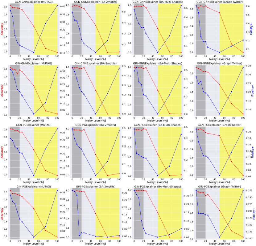
Due to space limit, the detailed evaluation (average results of three runs) is displayed in Table 2-3 of Appendix A. To facilitate the readers to understand our results, we partially summarise them into Figure 1. Dark grey and yellow shadows highlight the regions of and , respectively.
Q1. Post-hoc GNN explainers are susceptible to label noise. Figure 1 emphasises that both and are significantly impacted by varying levels of label noise. The fluctuating trends of (blue lines) underscore the instability of explanation quality, whereas the trends of (red lines) echo the findings about GNN robustness discussed in previous work [4, 5].
Observation 1. From the results in Table 2-3, we find out that decreases as increases from to . However, the definition of indicating lower values as more satisfactory contradicts this outcome. In our scenario, confusing labels lead to ambiguous predictions, subsequently causing . We thereby argue that proves unsuitable as a valid metric within the context of investigating post-hoc GNN explainer robustness.
Q2. The robustness of GNN models does not extend to the stable fidelity of post-hoc explainers. Within the grey shadow regions of Figure 1, it is evident that remains relatively stable, indicating that GNN models exhibit robustness in the face of minor noisy levels. Conversely, experiences substantial drops at the same noise levels (), revealing the heightened sensitivity of different post-hoc explainers to even minor noisy levels of label noise.
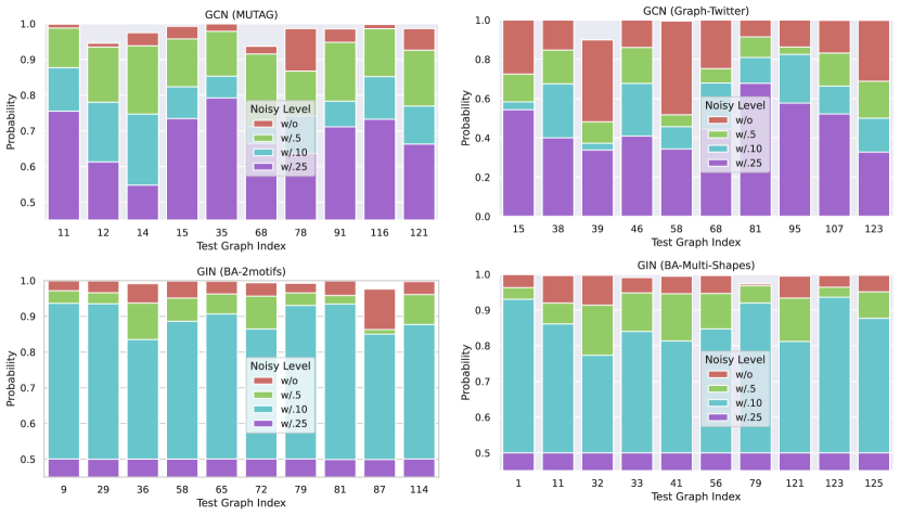
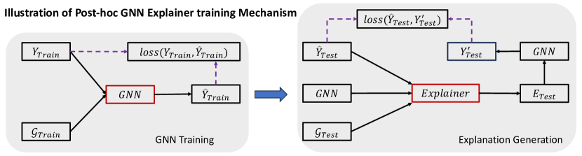
Observation 2. To unveil the grey shadow regions, we present the corresponding predicted probabilities of the true label of ten example test graphs in Figure 2. Although GNN models manage to accurately classify these graphs with minor noisy levels, yet, the predicted probabilities are affected by introduced noises, which are not represented in . In contrast, these predicted probabilities would be passed to GNN explainers as essential inputs to generate explanations, as illustrated in Figure 4. We posit that this might the chief reason for the contrasting performance of and .
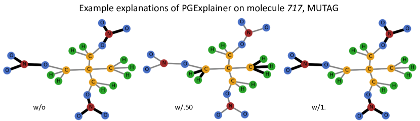
Observation 3. Another interesting phenomena we observed in Figure 1 is that beyond a noise threshold of 50%, gradually returns to levels comparable to those without noise as noise levels continue to escalate. To better understand this phenomenon, we present the generated explanations about an example molecule graph (id = 717) in Figure 3. At 50%, PGExplainer fails to identity key motifs (NO2), yet sucessfully does so at 100%. This suggests that confusing label signals mislead GNN models and explainers, while inverted label signals enables GNN models to predict reverse labels while identifying important features.
4 Concluding Remarks and Future Directions
This extended abstract represents, to the best of our knowledge, the first preliminary exploration into the robustness of post-hoc GNN explainers against label noise. Our findings introduce several interesting research questions to the community: Firstly, we establish the susceptibility of post-hoc GNN explainers to label noise. Secondly, our investigation highlights that the fidelity of post-hoc explainers can be significantly impacted by minor noise, which does not conduce a noticeable influence on the GNN model’s performance. This underscores the complexity inherent in bolstering the robustness of post-hoc GNN explainers, necessitating dedicated efforts. Additionally, our study unveils the impracticability of metric for explainer robustness study since it naturally gets optimised with high noisy levels. In follow-up work, there are several promising future directions to explore. For instance, designing robust post-hoc GNN explainers to label noise, refining explanation evaluation metrics for comprehensive measurement, and developing large-scale benchmark datasets.
Acknowledgements
This work is supported by the Horizon Europe and Innovation Fund Denmark under the Eureka, Eurostar grant no E115712 - AAVanguard.
References
- Wu et al. [2021] Zonghan Wu, Shirui Pan, Fengwen Chen, Guodong Long, Chengqi Zhang, and Philip S. Yu. A comprehensive survey on graph neural networks. IEEE Transactions on Neural Networks and Learning Systems (TNNLS), 32(1):4–24, 2021.
- Jegelka [2022] Stefanie Jegelka. Theory of graph neural networks: Representation and learning. CoRR, abs/2204.07697, 2022.
- Zhong et al. [2023a] Zhiqiang Zhong, Cheng-Te Li, and Jun Pang. Hierarchical message-passing graph neural networks. Data Mining and Knowledge Discovery (DMKD), 37(1):381–408, 2023a.
- Zügner et al. [2018] Daniel Zügner, Amir Akbarnejad, and Stephan Günnemann. Adversarial attacks on neural networks for graph data. In Proceedings of the 2018 ACM Conference on Knowledge Discovery and Data Mining (KDD), pages 2847–2856, 2018.
- Dai et al. [2018] Hanjun Dai, Hui Li, Tian Tian, Xin Huang, Lin Wang, Jun Zhu, and Le Song. Adversarial attack on graph structured data. In Proceedings of the 2018 International Conference on Machine Learning (ICML), volume 80, pages 1123–1132. PMLR, 2018.
- Zügner and Günnemann [2019] Daniel Zügner and Stephan Günnemann. Certifiable robustness and robust training for graph convolutional networks. In Proceedings of the 2019 ACM Conference on Knowledge Discovery and Data Mining (KDD), pages 246–256. ACM, 2019.
- Bojchevski and Günnemann [2019] Aleksandar Bojchevski and Stephan Günnemann. Certifiable robustness to graph perturbations. In Proceedings of the 2019 Annual Conference on Neural Information Processing Systems (NeurIPS), pages 8317–8328, 2019.
- Yuan et al. [2023] Hao Yuan, Haiyang Yu, Shurui Gui, and Shuiwang Ji. Explainability in graph neural networks: A taxonomic survey. IEEE Transactions on Pattern Analysis and Machine Intelligence (TPAMI), 45(5):5782–5799, 2023.
- Ying et al. [2019] Zhitao Ying, Dylan Bourgeois, Jiaxuan You, Marinka Zitnik, and Jure Leskovec. Gnnexplainer: Generating explanations for graph neural networks. In Proceedings of the 2019 Annual Conference on Neural Information Processing Systems (NeurIPS), pages 9240–9251, 2019.
- Luo et al. [2020] Dongsheng Luo, Wei Cheng, Dongkuan Xu, Wenchao Yu, Bo Zong, Haifeng Chen, and Xiang Zhang. Parameterized explainer for graph neural network. In Proceedings of the 2020 Annual Conference on Neural Information Processing Systems (NeurIPS), pages 19620–19631, 2020.
- Schlichtkrull et al. [2021] Michael Sejr Schlichtkrull, Nicola De Cao, and Ivan Titov. Interpreting graph neural networks for NLP with differentiable edge masking. In Proceedings of the 2021 International Conference on Learning Representations (ICLR), 2021.
- Pope et al. [2019] Phillip E. Pope, Soheil Kolouri, Mohammad Rostami, Charles E. Martin, and Heiko Hoffmann. Explainability methods for graph convolutional neural networks. In Proceedings of the 2014 Conference on Computer Vision and Pattern Recognition (CVPR), pages 10772–10781. IEEE, 2019.
- Schnake et al. [2023] Thomas Schnake, Oliver Eberle, Jonas Lederer, Shinichi Nakajima, Kristof T. Schütt, Klaus-Robert Müller, and Grégoire Montavon. Higher-order explanations of graph neural networks via relevant walks. IEEE Transactions on Pattern Analysis and Machine Intelligence (TPAMI), 44(11):7581–7596, 2023.
- Chen et al. [2022] Ninghan Chen, Xihui Chen, Zhiqiang Zhong, and Jun Pang. The burden of being a bridge: Analysing subjective well-being of twitter users during the COVID-19 pandemic. In Machine Learning and Knowledge Discovery in Databases - European Conference (ECMLPKDD), volume 13714, pages 241–257. Springer, 2022.
- Wang et al. [2023] Hanchen Wang, Tianfan Fu, Yuanqi Du, Wenhao Gao, Kexin Huang, Ziming Liu, Payal Chandak, Shengchao Liu, Peter Van Katwyk, Andreea Deac, et al. Scientific discovery in the age of artificial intelligence. Nature, 620(7972):47–60, 2023.
- Zhong et al. [2023b] Zhiqiang Zhong, Anastasia Barkova, and Davide Mottin. Knowledge-augmented graph machine learning for drug discovery: A survey from precision to interpretability. CoRR, abs/2302.08261, 2023b.
- Dai and Wang [2021] Enyan Dai and Suhang Wang. Towards self-explainable graph neural network. In Proceedings of the 2021 ACM International Conference on Information and Knowledge Management (CIKM), pages 302–311. ACM, 2021.
- Zhang et al. [2022] Zaixi Zhang, Qi Liu, Hao Wang, Chengqiang Lu, and Cheekong Lee. Protgnn: Towards self-explaining graph neural networks. In Proceedings of the 2022 AAAI Conference on Artificial Intelligence (AAAI), pages 9127–9135, 2022.
- Kipf and Welling [2017] Thomas N. Kipf and Max Welling. Semi-supervised classification with graph convolutional networks. In Proceedings of the 2017 International Conference on Learning Representations (ICLR), 2017.
- Xu et al. [2019] Keyulu Xu, Weihua Hu, Jure Leskovec, and Stefanie Jegelka. How powerful are graph neural networks? In Proceedings of the 2019 International Conference on Learning Representations (ICLR), 2019.
- Fey and Lenssen [2019] Matthias Fey and Jan E. Lenssen. Fast graph representation learning with pytorch geometric. In ICLR Workshop on Representation Learning on Graphs and Manifolds, 2019.
- Liu et al. [2021] Meng Liu, Youzhi Luo, Limei Wang, Yaochen Xie, Hao Yuan, Shurui Gui, Haiyang Yu, Zhao Xu, Jingtun Zhang, Yi Liu, Keqiang Yan, Haoran Liu, Cong Fu, Bora M Oztekin, Xuan Zhang, and Shuiwang Ji. DIG: A turnkey library for diving into graph deep learning research. Journal of Machine Learning Research, 22(240):1–9, 2021.
- Azzolin et al. [2022] Steve Azzolin, Antonio Longa, Pietro Barbiero, Pietro Liò, and Andrea Passerini. Global explainability of gnns via logic combination of learned concepts. CoRR, abs/2210.07147, 2022.
Appendix A Supplement Material
| Name | Cat. | #Graphs | #Nodes (Avg.) | #Edges (avg) | # Node Feat. | #Classes |
| MUTAG | Real | 4,337 | 30.3 | 61.5 | 14 | 2 |
| BA-2motifs | Syn. | 1,000 | 25 | 51 | 10 | 2 |
| BA-Multi-Shapes | Syn. | 1,000 | 25 | 51 | 10 | 2 |
| Graph-Twitter | Real | 6,940 | 21.1 | 40.2 | 768 | 3 |
Datasets. We consider four graph classification datasets as summarised in Table 1. MUTAG is a real-world dataset of 4,337 molecule graphs labelled according to their mutagenic effect [9]. Graph-Twitter is a real-world sentiment graph dataset of 6,940 text graphs, which is constructed based on text sentiment analysis [8]. BA-2motifs [10] and BA-Multi-Shapes [23] are two synthetic datasets of 1,000 random Barabasi-Albert (BA) graphs. Each graph of BA-2motifs is obtained by attaching either HouseMotif or CycleMotif. Each graph of BA-Multi-Shapes is obtained by attaching one of HouseMotif, WheelMotif and GridMotif. These graphs are assigned to one of the two classes according to the type of attached motifs. We split datasets into train/valid/test (, , ) subsets for the experiments. GNN models are trained on train datasets and test on test datasets.
Implementation Details. Our implementations mainly follows the settings of officially public Pytorch code of PGExplainer [10] (https://github.com/divelab/DIG/tree/main/dig/xgraph/PGExplainer). Particularly, we first train a GNN model (two-layers or three-layers of fixed hidden dimension 128) and select the one with the best . After, we pass trained GNN model, obtained predictions and the graph to the GNN explainers to ontain explanations and compute their and following https://github.com/divelab/DIG/tree/dig/benchmarks/xgraph. The learning rate to train GNN models and explainers is fixed as . Other settings follow the default their official implementations.
| Dataset | GNNExplainer | ||||||||||||
| GCN | GIN | ||||||||||||
| MUTAG | w/o | 0.818 | - | 0.375 | - | 0.425 | - | 0.821 | - | 0.365 | - | 0.367 | - |
| w/.25 | 0.768 | -6.1% | 0.142 | -62.1% | 0.144 | -66.1% | 0.766 | -6.7% | 0.163 | -55.3% | 0.161 | -56.1% | |
| w/.50 | 0.543 | -33.6% | 0.104 | -72.3% | 0.098 | -76.9% | 0.580 | -29.4% | 0.019 | -94.8% | 0.019 | -94.8% | |
| w/.75 | 0.244 | -70.2% | 0.290 | -22.7% | 0.288 | -32.2% | 0.254 | -69.1% | 0.106 | -71.0% | 0.110 | -70.0% | |
| w/1. | 0.189 | -76.9% | 0.405 | 8.0% | 0.399 | -6.1% | 0.213 | -74.1% | 0.381 | 4.4% | 0.381 | 3.8% | |
| BA-2motifs | w/o | 0.980 | - | 0.496 | - | 0.496 | - | 0.980 | - | 0.486 | - | 0.486 | - |
| w/.25 | 0.930 | -5.1% | 0.207 | -58.3% | 0.221 | -55.4% | 0.990 | 1.0% | 0.205 | -57.8% | 0.204 | -58.0% | |
| w/.50 | 0.575 | -41.3% | 0.129 | -74.0% | 0.164 | -66.9% | 0.505 | -48.5% | -0.002 | -100.4% | -0.002 | -100.4% | |
| w/.75 | 0.000 | -100.0% | 0.235 | -52.6% | 0.235 | –52.6% | 0.000 | -100.0% | 0.209 | -57.0% | 0.200 | -58.8% | |
| w/1. | 0.010 | -99.0% | 0.554 | 11.7% | 0.556 | 12.1% | 0.005 | -99.5% | 0.477 | -1.9% | 0.476 | -2.1% | |
| BAMult.S. | w/o | 0.970 | - | 0.479 | - | 0.479 | - | 0.990 | - | 0.488 | - | 0.488 | - |
| w/.25 | 0.955 | -1.5% | 0.230 | -52.0% | 0.223 | -53.4% | 0.985 | -0.5% | 0.206 | -57.8% | 0.202 | -58.6% | |
| w/.50 | 0.510 | -47.4% | 0.031 | -93.5% | 0.050 | -89.6% | 0.505 | -49.0% | 0.002 | -99.6% | 0.002 | -99.6% | |
| w/.75 | 0.010 | -99.0% | 0.204 | -57.4% | 0.198 | -58.7% | 0.005 | -99.5% | 0.217 | -55.5% | 0.212 | -56.6% | |
| w/1. | 0.000 | -100.0% | 0.522 | 9.0% | 0.528 | 10.2% | 0.000 | -100.0% | 0.480 | -1.6% | 0.479 | -1.8% | |
| G.-Twitter | w/o | 0.635 | - | 0.605 | - | 0.594 | - | 0.665 | - | 0.286 | - | 0.262 | - |
| w/.25 | 0.616 | -3.0% | 0.161 | -73.4% | 0.162 | -72.7% | 0.613 | -7.8% | 0.182 | -36.4% | 0.173 | -34.0% | |
| w/.50 | 0.556 | -12.4% | 0.055 | -90.9% | 0.054 | -90.9% | 0.476 | -28.4% | 0.074 | -74.1% | 0.070 | -73.3% | |
| w/.75 | 0.194 | -69.4% | 0.012 | -98.0% | 0.012 | -98.0% | 0.276 | -58.5% | 0.201 | -29.7% | 0.197 | -24.8% | |
| w/1. | 0.097 | -84.7% | 0.121 | -80.0% | 0.120 | -79.8% | 0.162 | -75.6% | 0.341 | 19.2% | 0.309 | 17.9% | |
| Dataset | PGExplainer | ||||||||||||
| MUTAG | w/o | 0.809 | - | 0.307 | - | 0.431 | - | 0.823 | - | 0.330 | - | 0.482 | - |
| w/.25 | 0.767 | -5.2% | 0.203 | -33.9% | 0.274 | -36.4% | 0.741 | -10.0% | 0.123 | -62.7% | 0.117 | -75.7% | |
| w/.50 | 0.531 | -34.4% | 0.043 | -86.0% | 0.094 | -78.2% | 0.580 | -29.5% | 0.003 | -99.1% | 0.013 | -97.3% | |
| w/.75 | 0.254 | -68.6% | 0.233 | -24.1% | 0.287 | -33.4% | 0.280 | -66.0% | 0.084 | -74.5% | 0.041 | -91.5% | |
| w/1. | 0.188 | -76.8% | 0.377 | 22.8% | 0.443 | 2.8% | 0.188 | -77.2% | 0.366 | 10.9% | 0.406 | -15.8% | |
| BA-2motifs | w/o | 0.995 | - | 0.489 | - | 0.489 | - | 1.000 | - | 0.316 | - | 0.481 | - |
| w/.25 | 0.985 | -1.0% | 0.210 | -57.1% | 0.213 | -56.4% | 0.985 | -1.5% | 0.024 | -92.4% | 0.210 | -56.3% | |
| w/.50 | 0.445 | -55.3% | -0.024 | -104.9% | 0.193 | -60.5% | 0.505 | -49.5% | -0.000 | -100.0% | -0.000 | -100.0% | |
| w/.75 | 0.000 | -100.0% | 0.129 | -73.6% | 0.147 | -69.9% | 0.005 | -99.5% | -0.006 | -101.9% | 0.209 | -56.5% | |
| w/1. | 0.045 | -95.5% | 0.467 | -4.5% | 0.489 | 0.0% | 0.010 | -99.0% | 0.006 | -98.1% | 0.463 | -3.7% | |
| BAMult.S. | w/o | 0.980 | - | 0.482 | - | 0.482 | - | 0.985 | - | 0.281 | - | 0.485 | - |
| w/.25 | 0.980 | 0.0% | 0.214 | -55.6% | 0.252 | -47.7% | 0.975 | -1.0% | 0.022 | -92.2% | 0.143 | -70.5% | |
| w/.50 | 0.455 | -53.6% | 0.055 | -88.6% | 0.108 | -77.6% | 0.520 | -47.2% | 0.001 | -99.6% | 0.002 | -99.6% | |
| w/.75 | 0.005 | -99.5% | 0.140 | -71.0% | 0.144 | -70.1% | 0.000 | -100.0% | 0.016 | -94.3% | 0.237 | -51.1% | |
| w/1. | 0.020 | -98.0% | 0.433 | -10.2% | 0.443 | -8.1% | 0.000 | -100.0% | 0.051 | -81.9% | 0.501 | 3.3% | |
| G.-Twitter | w/o | 0.633 | - | 0.209 | - | 0.333 | - | 0.656 | - | 0.275 | - | 0.255 | - |
| w/.25 | 0.587 | -7.3% | 0.120 | -42.6% | 0.157 | -52.9% | 0.610 | -7.0% | 0.185 | -32.7% | 0.174 | -31.8% | |
| w/.50 | 0.558 | -11.8% | 0.063 | -69.9% | 0.062 | -81.4% | 0.429 | -34.6% | 0.105 | -61.8% | 0.030 | -88.2% | |
| w/.75 | 0.256 | -59.6% | 0.136 | -34.9% | 0.263 | -21.0% | 0.195 | -70.3% | 0.172 | -37.5% | 0.172 | -32.5% | |
| w/1. | 0.092 | -85.5% | 0.206 | -1.4% | 0.307 | -7.8% | 0.123 | -81.3% | 0.274 | -0.4% | 0.276 | 8.2% | |
| Dataset | GNNExplainer | ||||||||||||
| GCN | GIN | ||||||||||||
| MUTAG | w/o | 0.818 | - | 0.375 | - | 0.425 | - | 0.821 | - | 0.365 | - | 0.367 | - |
| w/.5 | 0.798 | -2.4% | 0.337 | -10.1% | 0.334 | -21.4% | 0.798 | -2.8% | 0.344 | -5.8% | 0.336 | -8.4% | |
| w/.10 | 0.790 | -3.4% | 0.212 | -43.5% | 0.215 | -49.4% | 0.794 | -3.3% | 0.285 | -21.9% | 0.276 | -24.8% | |
| w/.15 | 0.787 | -3.8% | 0.166 | -55.7% | 0.171 | -59.8% | 0.737 | -10.2% | 0.208 | -43.0% | 0.204 | -44.4% | |
| w/.20 | 0.778 | -4.9% | 0.151 | -59.7% | 0.156 | -63.3% | 0.786 | -4.3% | 0.195 | -46.6% | 0.192 | -47.7% | |
| BA-2motifs | w/o | 0.980 | - | 0.496 | - | 0.496 | - | 0.980 | - | 0.486 | - | 0.486 | - |
| w/.5 | 0.990 | 1.0% | 0.423 | -14.7% | 0.397 | -20.0% | 0.985 | 0.5% | 0.440 | -9.5% | 0.439 | -9.7% | |
| w/.10 | 0.990 | 1.0% | 0.415 | -16.3% | 0.389 | -21.6% | 0.995 | 1.5% | 0.364 | -25.1% | 0.363 | -25.3% | |
| w/.15 | 0.970 | -1.0% | 0.345 | -30.4% | 0.342 | -31.0% | 0.965 | -1.5% | 0.274 | -43.6% | 0.274 | -43.6% | |
| w/.20 | 0.950 | -3.1% | 0.248 | -50.0% | 0.250 | -49.6% | 0.970 | -1.0% | 0.231 | -52.5% | 0.230 | -52.7% | |
| BAMult.S. | w/o | 0.970 | - | 0.479 | - | 0.479 | - | 0.990 | - | 0.488 | - | 0.488 | - |
| w/.5 | 0.980 | 1.0% | 0.392 | -18.2% | 0.437 | -8.8% | 0.985 | -0.5% | 0.530 | 8.6% | 0.429 | -12.1% | |
| w/.10 | 0.980 | 1.0% | 0.335 | -30.1% | 0.313 | -34.7% | 0.980 | -1.0% | 0.365 | -25.2% | 0.363 | -25.6% | |
| w/.15 | 0.975 | 0.5% | 0.294 | -38.6% | 0.294 | -38.6% | 0.985 | -0.5% | 0.334 | -31.6% | 0.333 | -31.8% | |
| w/.20 | 0.990 | 2.1% | 0.294 | -38.6% | 0.298 | -37.8% | 0.960 | -3.0% | 0.218 | -55.3% | 0.228 | -53.3% | |
| G.-Twitter | w/o | 0.635 | - | 0.605 | - | 0.594 | - | 0.665 | - | 0.286 | - | 0.262 | - |
| w/.5 | 0.612 | -3.6% | 0.523 | -13.6% | 0.515 | -13.3% | 0.651 | -2.1% | 0.247 | -13.6% | 0.229 | -12.6% | |
| w/.10 | 0.638 | 0.5% | 0.244 | -59.7% | 0.244 | -58.9% | 0.639 | -3.9% | 0.261 | -8.7% | 0.246 | -6.1% | |
| w/.15 | 0.623 | -1.9% | 0.192 | -68.3% | 0.189 | -68.2% | 0.620 | -6.9% | 0.202 | -29.4% | 0.192 | -26.7% | |
| w/.20 | 0.635 | 0.0% | 0.186 | -69.3% | 0.187 | -68.5% | 0.619 | -6.9% | 0.194 | -32.2% | 0.189 | -27.9% | |
| Dataset | PGExplainer | ||||||||||||
| MUTAG | w/o | 0.809 | - | 0.307 | - | 0.431 | - | 0.823 | - | 0.330 | - | 0.482 | - |
| w/.5 | 0.807 | -0.2% | 0.294 | -4.2% | 0.366 | -15.1% | 0.780 | -5.2% | 0.281 | -14.8% | 0.308 | -36.1% | |
| w/.10 | 0.789 | -2.5% | 0.249 | -18.9% | 0.322 | -25.3% | 0.786 | -4.5% | 0.261 | -20.9% | 0.262 | -45.6% | |
| w/.15 | 0.787 | -2.7% | 0.236 | -23.1% | 0.316 | -26.7% | 0.767 | -6.8% | 0.200 | -39.4% | 0.193 | -60.0% | |
| w/.20 | 0.767 | -5.2% | 0.206 | -32.9% | 0.294 | -31.8% | 0.759 | -7.8% | 0.144 | -56.4% | 0.132 | -72.6% | |
| BA-2motifs | w/o | 0.995 | - | 0.489 | - | 0.489 | - | 1.000 | - | 0.316 | - | 0.481 | - |
| w/.5 | 0.973 | -2.2% | 0.380 | -22.3% | 0.420 | -14.1% | 0.975 | -2.5% | 0.310 | -1.9% | 0.446 | -7.3% | |
| w/.10 | 0.971 | -2.4% | 0.320 | -34.6% | 0.331 | -32.3% | 0.995 | -0.5% | 0.282 | -10.8% | 0.378 | -21.4% | |
| w/.15 | 0.970 | -2.5% | 0.284 | -41.9% | 0.285 | -41.7% | 0.985 | -1.5% | 0.004 | -98.7% | 0.343 | -28.7% | |
| w/.20 | 0.950 | -4.5% | 0.267 | -45.4% | 0.282 | -42.3% | 0.980 | -2.0% | 0.023 | -92.7% | 0.240 | -50.1% | |
| BAMult.S. | w/o | 0.980 | - | 0.482 | - | 0.482 | - | 0.985 | - | 0.281 | - | 0.485 | - |
| w/.5 | 0.965 | -1.5% | 0.258 | -46.5% | 0.360 | -25.3% | 0.980 | -0.5% | 0.257 | -8.5% | 0.438 | -9.7% | |
| w/.10 | 0.970 | -1.0% | 0.246 | -49.0% | 0.253 | -47.5% | 0.985 | 0.0% | 0.236 | -16.0% | 0.288 | -40.6% | |
| w/.15 | 0.955 | -2.6% | 0.228 | -52.7% | 0.229 | -52.5% | 0.985 | 0.0% | 0.102 | -63.7% | 0.326 | -32.8% | |
| w/.20 | 0.958 | -2.2% | 0.218 | -54.8% | 0.218 | -54.8% | 0.985 | 0.0% | 0.051 | -81.9% | 0.271 | -44.1% | |
| G.-Twitter | w/o | 0.633 | - | 0.209 | - | 0.333 | - | 0.656 | - | 0.275 | - | 0.255 | - |
| w/.5 | 0.633 | 0.0% | 0.168 | -19.6% | 0.213 | -36.0% | 0.638 | -2.7% | 0.192 | -30.2% | 0.175 | -31.4% | |
| w/.10 | 0.638 | 0.8% | 0.149 | -28.7% | 0.186 | -44.1% | 0.629 | -4.1% | 0.191 | -30.6% | 0.174 | -31.8% | |
| w/.15 | 0.619 | -2.2% | 0.125 | -40.2% | 0.178 | -46.6% | 0.632 | -3.7% | 0.191 | -30.6% | 0.188 | -26.3% | |
| w/.20 | 0.594 | -6.2% | 0.124 | -40.7% | 0.161 | -51.7% | 0.596 | -9.2% | 0.186 | -32.4% | 0.176 | -31.0% | |