Suppression of small-scale dynamo in time irreversible turbulence

Abstract

The conventional theory of small-scale magnetic field generation in a turbulent flow considers time-reversible random flows. However, real turbulent flows are known to be time irreversible: the presence of energy cascade is an intrinsic property of turbulence. We generalize the ’standard’ model to account for the irreversibility. We show that even small time asymmetry leads to significant suppression of the dynamo effect at low magnetic Prandtl numbers, increases the generation threshold and may even make generation impossible for any magnetic Reynolds number. We calculate the magnetic energy growth rate as a function of the parameters of the flow.

1 Introduction

The theory of magnetic field generation in a turbulent flow has numerous applications and, in particular, is likely to explain the existence of magnetic field in many astrophysical objects (Parker, 1979; Brandenburg & Subramanian., 2005; Sokoloff, 2015; Kuznetsov & Mikhailov, 2022; Hazra et al., 2023). The basic idea of turbulent dynamo is that the magnetic lines stretch as they are carried by turbulent motion. However, a very wide range of magnetized astrophysical objects of different scales implies very different parameters of the medium. A small-scale turbulent dynamo, i.e., a dynamo that takes place at scales much smaller than the integral scale of turbulence (Batchelor, 1950; Falkovich et al., 2001; Brandenburg et al., 2012), depends on two basic parameters: the hydrodynamic Reynolds number Re and the magnetic Reynolds number Rm. Their ratio Rm/Re=Pm is called magnetic Prandtl number: it indicates whether the viscous scale $r_{\nu}$ of turbulence is larger (Pm$>1$) or smaller than the resistive scale $r_{d}$. While both Rm and Re are large in cosmic plasmas, their ratio varies crucially, and Pm is either very large or very small in astrophysical objects. The Prandtl number controls the small-scale dynamo mechanism (Batchelor, 1950; Rincon, 2019).

The high-Pm turbulence is observed in interstellar and intergalactic media (Rincon, 2019; Han, 2017). In these objects, the characteristic scale of magnetic field generation is deep inside the viscous range of turbulence, so the stretching of magnetic lines is exponential (Vainshtein & Zel’dovich, 1972); the existence of the dynamo effect for this case is confirmed by different theoretical approaches (Falkovich et al., 2001; Chertkov et al., 1999; Kazantsev, 1968) and by numerical simulations (Schekochihin et al., 2004; Brandenburg et al., 2023).

To the contrary, in stellar and planetary magnetism, in protostellar disks etc., one observes low-Pm media Pm $\sim 10^{-3}\div 10^{-7}$ (Rincon, 2019; Rempel et al., 2023). In this case, small-scale dynamo can occur only in the inertial range of turbulence, at scales $\rho\gtrsim r_{d}\gg r_{\nu}$. The existence of this effect is still questionable. Direct numerical simulations (DNS) are very difficult to perform in this range of parameters (Iskakov et al., 2007; Brandenburg et al., 2018); some authors report the existence of generation, and even the existence of a universal limit Rm_c that guarantees the dynamo for any Re (Schekochihin et al., 2007; Warnecke et al., 2023), although their estimates for the threshold Rm_c differ essentially, and the values of Pm and especially Re that they achieve (Pm$\gtrsim 10^{-3}$, Re$\lesssim 10^{5}$) are still far from the observed in astrophysic objects. Simulations performed by means of the shell model (Buchlin, 2011; Verma & Kumar, 2016; Plunian et al., 2013) and the implicit large-eddy simulations (Rempel, 2014; Hotta et al., 2016; Köpylö et al., 2018; Rempel et al., 2023) allow to get small-scale dynamo at more realistic parameters, however, the results may depend significantly on the model assumptions (Haugen & Brandenburg., 2006; Miesch et al., 2015). Observations of the Sun show the presence of small-scale magnetic field, but it is unclear whether it is, indeed, generated in the inertial range by turbulent motion (Petrovay & Szakaly, 1993), or it is merely a result of fragmentation of the large-scale field produced by some other process; Stenflo (2012a, b) argues that the latter is more likely. Theoretical consideration predicts the possibility of the dynamo effect in the low-Pm limit (Vainstein, 1982). Kazantsev has found the dependence of the growth rate on the scaling properties of isotropic incompressible flow with infinite Re (infinite integral scale of turbulence), under the assumption of Gaussian and delta correlated velocity statistics. In later papers, the model was extended for the case of finite Re (Novikov et al., 1983; Vainshtein & Kichatinov, 1986; Rogachevskii & Kleeorin, 1997; Vincenzi, 2002; Arponen & Horvai, 2007; Boldyrev & Cattaneo, 2004; Malyshkin & Boldyrev, 2010; Schober et al., 2012; Istomin & Kiselev, 2013).

However, these theoretical works consider only time-reversible random flows. Actually, the time asymmetry is associated with the third-order velocity correlator, which is zero in the classical Kazantsev model. Meanwhile, the real turbulent flows are known to be time irreversible: this follows from the existence of energy cascade (Kolmogorov, 1941; Frisch, 1995). The account of small time irreversibility in the high-Pm limit has shown the decrease of all magnetic field statistical moments growth rate (Kopyev et al., 2022b; Zybin et al., 2020; Il’yn et al., 2020). So, there is a reasonable question: how does it affect the magnetic field generation in the low-Pm case?

In this article, we consider the influence of the time irreversibility of turbulence on the ability of a low-Pm conductive fluid to generate magnetic field. We find the instability criterion and show that the magnetic generation in a turbulent flow may be suppressed completely if the third order correlator is large enough. We show that in this case, even for infinite Rm, there is no generation for Pm small enough but finite.

2 Definitions and the $V^{3}$ model

The evolution of magnetic field in a (random) velocity field $\textbf{{v}}({\textbf{{r}}},t)$ is described by the equation

$$\frac{\partial\textbf{{B}}(\textbf{{r}},t)}{\partial t}=\mathrm{rot}\bigl{[}\textbf{{v}}(\textbf{{r}},t)\times\textbf{{B}}(\textbf{{r}},t)\bigr{]}+\eta\Delta\textbf{{B}}(\textbf{{r}},t)$$ (1)

where $\eta$ is the magnetic diffusivity. The magnetic field energy in the problems under consideration is smaller than the kinetic energy of the flow at all scales, and the feedback influence of the magnetic field on the velocity dynamics is proportional to $B^{2}$, so one can neglect this feedback and consider ${\textbf{{v}}}({\textbf{{r}}},t)$ as stationary random process with given statistics.

We consider isotropic and homogenous stationary flow in incompressible fluid. The Kazantsev equation for the second-order magnetic field correlator was derived for Gaussian $\delta$-correlated in time velocity field,

$$\langle v_{i}(\textbf{{r}},t)v_{j}(\textbf{{r}}_{1},t_{1})\rangle=D_{ij}(\textbf{{r}}-\textbf{{r}}_{1})\,\delta_{\epsilon}(t-t_{1})$$ (2)

Here $\delta_{\epsilon}$ is not a ’physical’ singularity but a regularized $\delta$ function: a narrow peak with unitary square and width smaller than all physical scales. To avoid ambiguities, for any real (short-correlated) velocity field one can define $D_{ij}$ by the integral

$$D_{ij}(\boldsymbol{\rho})=\int\langle v_{i}(\textbf{{r}},t)v_{j}(\textbf{{r}}+\boldsymbol{\rho},t+\tau)\rangle\mathrm{d}\tau$$ (3)

(It does not depend on r and $t$ because of space and time homogeneity.) To take account of the third-order velocity correlator, we introduce

$$F_{ijk}(\boldsymbol{\rho}_{1},\boldsymbol{\rho}_{2})=\int\langle v_{i}(\textbf{{r}},t)v_{j}(\textbf{{r}}+\boldsymbol{\rho}_{1},t_{1})v_{k}(\textbf{{r}}+\boldsymbol{\rho}_{2},t_{2})\rangle\mathrm{d}t_{1}\mathrm{d}t_{2}$$ (4)

Now we use the $V^{3}$ model (Il’yn et al., 2016; Kopyev et al., 2022b, a). It is a generalization of the Kazantsev-Kraichnan model (Kazantsev, 1968; Kraichnan & Nagarajan, 1967) and implies two assumptions: 1) the third order correlator is assumed to be singular in time:

$$\langle v_{i}(\textbf{{r}},t)v_{j}(\textbf{{r}}+\boldsymbol{\rho}_{1},t_{1})v_{k}(\textbf{{r}}+\boldsymbol{\rho}_{2},t_{2})\rangle=F_{ijk}(\boldsymbol{\rho}_{1},\boldsymbol{\rho}_{2})\frac{\delta_{\epsilon}(t-t_{1})\delta_{\epsilon}(t-t_{2})+\delta_{\epsilon}(t-t_{1})\delta_{\epsilon}(t_{1}-t_{2})+\delta_{\epsilon}(t-t_{2})\delta_{\epsilon}(t_{1}-t_{2})}{3},$$ (5)

and 2) the higher order correlators are set to zero. We will discuss the validity of these assumptions a few strings later.

Under these assumptions, we derive the generalized Kazantsev equation (see Appendix A for derivation):

$$\frac{\partial}{\partial t}G= \,2\eta\left(G^{\prime\prime}_{\rho\rho}+\frac{4G^{\prime}_{\rho}}{\rho}\right)+bG^{\prime\prime}_{\rho\rho}+\left(b^{\prime}+4\frac{b}{\rho}\right)G^{\prime}_{\rho}+\left(b^{\prime\prime}+4\frac{b^{\prime}}{\rho}\right)G+$$ (6)

$$2cG^{\prime\prime\prime}_{\rho\rho\rho}+3\left(c^{\prime}+\frac{4c}{\rho}\right)G^{\prime\prime}_{\rho\rho}+\left(3c^{\prime\prime}+\frac{12c^{\prime}}{\rho}+\frac{8c}{\rho^{2}}+\frac{8d}{\rho}\right)G^{\prime}_{\rho}+\left(c^{\prime\prime\prime}+\frac{6c^{\prime\prime}}{\rho}+\frac{4c^{\prime}}{\rho^{2}}-\frac{4c}{\rho^{3}}+\frac{4d^{\prime}}{\rho}+\frac{12d}{\rho^{2}}\right)G$$

Here

$$G(\rho,t)=\langle B_{L}(\textbf{{r}}+\boldsymbol{\rho},t)B_{L}(\textbf{{r}},t)\rangle$$ (7)

is the magnetic field correlator, and

$$\begin{array}[]{l}b(\rho)={n}_{i}{n}_{j}\left(D_{ij}(0)-D_{ij}(\boldsymbol{\rho})\right),\\ c(\rho)=\tfrac{1}{2}{n}_{i}\Pi_{jk}F_{ijk}(\boldsymbol{\rho},\boldsymbol{\rho}),\\ d(\rho)=-\left(\tfrac{1}{8}n_{i}n_{j}\Pi_{kl}+\tfrac{1}{2}n_{j}n_{l}\Pi_{ik}\right)\frac{\partial}{\partial{\rho_{1}}_{l}}F_{ijk}(\boldsymbol{\rho}_{1},\boldsymbol{\rho})\bigl{|}_{\boldsymbol{\rho}_{1}=\boldsymbol{\rho}},\\ \textbf{{n}}=\boldsymbol{\rho}/\rho\ ,\ \ \Pi_{ij}=\delta_{ij}-n_{i}n_{j}\ ,\ \ B_{L}=\textbf{{B}}\cdot{\textbf{{n}}}\end{array}$$ (8)

represent the velocity correlators.

The applicability of the first assumption in long-term asymptotics for smooth velocity field (Batchelor regime, $\rho<r_{\nu}$) was proved by Il’yn et al. (2022). For rough velocity field (inertial range, $\rho>r_{\nu}$) the correctness of this assumption remains a hypothesis: we suppose that the effect of the finite correlation time is weaker than that of the asymmetry. The insignificance of the finite-correlation time corrections for the Kazantsev model was confirmed in DNS (Mason et al., 2011).

The second assumption produces non-physical artefacts, as any non-Gaussian model with a finite number of cumulants does (Klyatskin, 2005; Millionschikov, 1941; Monin & Yaglom, 1987). Specifically, Eq. (6) contains the third order derivative, while the Kazantsev equation ($c=d=0$) is the second order differential equation. So, in addition to corrections to the two ’Kazantsev’ modes, Eq. (6) provides a new eigenmode that is non-physical. The account of the whole set of the higher order correlators would destroy this ’parasite’ mode, but one can choose them small enough to have no significant effect on the two ’physical’ modes.

For large Pm, it is enough to restrict the consideration by the viscous scales range. Eq.(6) then reduces to the equation derived by Kopyev et al. (2022b). For small Pm, careful analysis of the inertial range is needed.

3 Rough velocity field

In the inertial range of hydrodynamical turbulence, $b(\rho)\propto\rho^{4/3}$; indeed, for Kolmogorov turbulence (Vainstein, 1982; Vainshtein & Kichatinov, 1986; Rogachevskii & Kleeorin, 1997) one has

$$\delta v(\rho)\propto\rho^{1/3},\,\,\tau_{c}(\rho)\propto\rho/\delta v\propto\rho^{2/3}\,\Rightarrow\,\,b(\rho)\propto\delta v^{2}\tau_{c}\propto\rho^{4/3}$$ (9)

Following Kazantsev, we hereafter consider a more general rough velocity field with the power-law structure function $b(\rho)\propto\rho^{1+s}$. From dimensional analysis we then get

$$\left\{\begin{aligned} &\delta v(\rho)\propto\rho^{s}\\ &\tau_{c}(\rho)\propto\rho^{1-s}\end{aligned}\right.\Rightarrow\left\{\begin{aligned} b(\rho)&&\propto&&\rho^{1+s}\\ c(\rho)&&\propto&&\zeta\,\rho^{2+s}\\ d(\rho)&&\propto&&-\beta\,\zeta\,\rho^{1+s},\end{aligned}\right.$$ (10)

Thus, we define

$$\zeta=\frac{c(\rho)}{\rho\,b(\rho)}\ ,\ \zeta\beta=-\frac{d(\rho)}{b(\rho)}$$ (11)

The $\zeta$ and $\beta$ are dimensionless parameters that characterize the third order correlator and that are constants inside the hydrodynamic inertial range of scales; $\zeta$ must be small to ensure the applicability of the $V^{3}$ model, while $\beta$ is, generally, not restricted. From Kopyev & Zybin (2018) analysis of numerical simulations Li et al. (2008); Yeung et al. (2012) it follows that $\beta\simeq 2$. We note that in (10),(11) we neglect possible intermittency: there is no evidence of anomalous scaling for time-integrated functions.

We also introduce the convenient length scale

$$r_{d}=\rho\left(2\eta/b(\rho)\right)^{1/(1+s)}\ ,\rho\gg r_{\nu}$$ (12)

For $\rho\gg r_{d}$, the molecular diffusion is negligibly small, and one can omit the first bracket in (6). Then

$$\frac{1}{2\eta}\frac{\partial}{\partial t}G= \left(\frac{\rho}{r_{d}}\right)^{1+s}\left(G^{\prime\prime}+\frac{5+s}{\rho}G^{\prime}+\frac{(4+s)(1+s)}{\rho^{2}}G\right)+$$ (13)

$$\zeta\,\left(\frac{\rho}{r_{d}}\right)^{1+s}\biggl{(}2\rho\,G^{\prime\prime\prime}+({18+3s})G^{\prime\prime}+\frac{3(5+s)(2+s)-8(\beta-1)}{\rho}G^{\prime}\left.+\frac{(4+s)\bigl{(}(4+s)(1+s)-4\beta\bigr{)}}{\rho^{2}}G\right),\ \rho\gg r_{d}$$

4 Generation threshold

In the case $\zeta=0$, (6) turns into the Kazantsev equation. The magnetic field generation in this model is possible for $s>0$, while for $s\leq 0$ the magnetic field decreases (Kazantsev, 1968). Indeed, setting $\frac{\partial}{\partial t}G=0$ in (13) we get two stationary modes, which for $\rho\gg r_{d}$ obey the scaling law:

$$G=\rho^{-\frac{s+4}{2}}\left(C_{+}\rho^{\mu_{K+}}+C_{-}\rho^{\mu_{K-}}\right)\ ,\mu_{K\pm}=\pm\frac{\sqrt{3}}{2}\sqrt{-s(s+4)}$$ (14)

The exponential in time solutions

$$G=e^{\Gamma t}G(\rho)\ ,\partial G/\partial t=\Gamma G$$ (15)

of the Kazantsev equation exist if and only if the stationary solution oscillates in space. (This can be derived from the oscillation theorem, keeping in mind that the Kazantsev equation reduces to a Schr$\ddot{{\rm o}}$dinger equation; less formally, this implies that the solution (14) must match both with the ’viscous’ solution at $\rho<r_{d}$ and with the large-scale solution at $\rho\to\infty$.)

We now use the same approach to find the magnetic field generation threshold for $\zeta\neq 0$. Taking $\rho\gg r_{d}$ for the stationary mode of (13) we get the power-law solutions $G\propto\rho^{-\frac{s+4}{2}+\mu_{\pm}}$ with the characteristic equation for the powers $\mu_{\pm}$:

$$\chi(\mu)=\left(\mu^{2}+\frac{3}{4}s(s+4)\right)\left(1+2\zeta\mu\right)-8\zeta\beta\mu=0$$ (16)

Two of the solutions are close to those found for $\zeta=0$. The third solution is $\sim\zeta^{-1}$, and it is a non-physical artefact. Again, the existence of generation corresponds to oscillating stationary mode eigenfunctions, i.e., to imaginary roots of (16). The minimum of the function $\chi(\mu)$, to the second order in $\zeta$, is

$$\chi_{min}=\frac{3}{4}s(s+4)-\zeta^{2}\left(4\beta-\frac{3}{4}s(s+4)\right)^{2}$$ (17)

We see that the presence of $\zeta$ of any sign lowers the minimum. The generation is still possible if $\chi_{min}>0$, i.e., if

$$|\zeta|<\zeta_{cr}=\frac{\sqrt{\frac{3}{4}s(s+4)}}{|4\beta-\frac{3}{4}s(s+4)|}\simeq\frac{\sqrt{3s}}{4|\beta|}$$ (18)

For $s=1/3$, $\beta=2$ we get $\zeta_{cr}\simeq 1/7$. For larger $\zeta$, there is no dynamo.

We note that the role of $\beta$ is crucial: actually, one can see from (16) that the terms $\zeta\beta$ are more effective to damp the oscillations than the terms with $\zeta$ alone. This means that the contribution of $d(\rho)$ in (6) is more important than of $c(\rho)$.

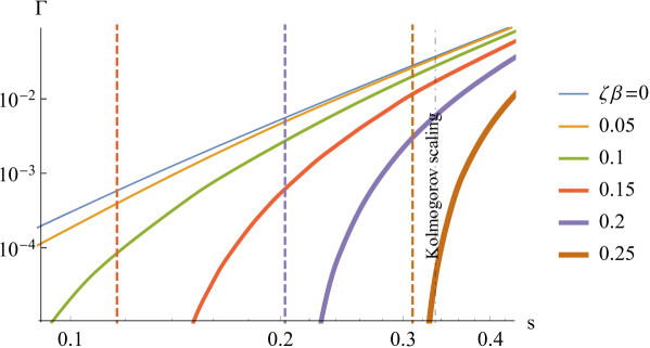
Figure 1: The maximal growh rate $\Gamma$ as a function of $s$ for different values $\zeta\beta$ in the minimal $V^{3}$ model; $\Gamma$ is normalized by $DPm^{(1-s)/(1+s)}$ where $D$ is characteristic frequency of small-scale eddies, $D=-\frac{3}{4}\left.\frac{\partial^{2}}{\partial\rho^{2}}\langle v_{L}(\boldsymbol{\rho})v_{L}({\bf 0})\rangle\right|_{\rho=0}$.

5 Growth rate

Even if the generation is not completely suppressed, its rate can be significantly slowed down. To investigate the dependence of the generation rate on the time irreversibility, we focus on the terms in (6) that contain $d$, and set $c=0$. We call this ’minimal model’. The estimate of $\zeta_{cr}$ obtained in the ’minimal model’ coincides with (18) to the first order in $s$.

We are looking for exponentially growing solutions (15). Now, the ’minimal model’ equation is a second-order ordinary differential equation containing the growth rate $\Gamma$; it has a discrete spectrum of solutions for $\Gamma>0$ if $\zeta$ satisfies (18).

By means of the method proposed by Il’yn et al. (2021, Appendix A), we find numerically the maximal possible $\Gamma$ for given $s$ and $\zeta$, assuming $\beta=2$. We normalize it by $Pm^{\frac{1-s}{1+s}}$, so that it becomes independent of the regularization as Pm$\to 0$ (Schober et al., 2012). The results are presented in Fig.1. We see that they differ significantly from the Kazantsev case: for $s=1/3$ the generation suppression is essential even for $\zeta\beta\lesssim 0.2$. The vertical asymptotes in the logarithmic coordinates correspond to the generation threshold. The dependence of the critical value of $\zeta\beta$ on $s$ is given in Fig.2. (For analytical expression, see Appendix B.) It confirms a good agreement between the $V^{3}$ and the ’minimal’ $V^{3}$ models (with and without $c(\rho)$) up to $s=1/3$. The whole analysis is performed in the limit of infinite integral scale, i.e., Rm$=\infty$; thus, from Fig.2 it follows that, in the frame of our model, for $\zeta\beta\gtrsim 1/3$ generation is impossible for any magnetic Reynolds number if Pm is small enough.

6 Conclusion

Summarizing, the presence of even small irreversibility is shown to suppress partially or completely the small-scale magnetic field generation in the case of small Prandtl numbers. The mixed velocity and gradients correlator $d(\rho)$ is shown to play a crucial role in this anti-dynamo effect. The effect is strong enough to be significant, e.g., for small-scale dynamo in convection zones of Sun and other stars, and perhaps in protostellar disks. For large Pm (galaxies, galaxy clusters) the analogous effect is weaker and cannot suppress dynamo completely (Kopyev et al., 2022b).

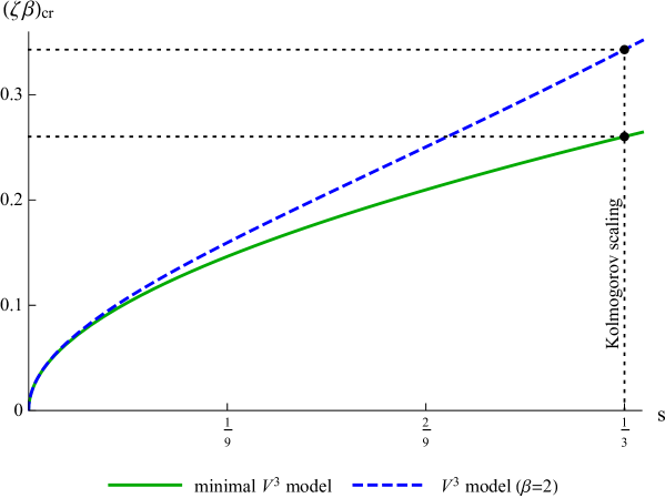
Figure 2: The critical value $(\zeta\beta)_{cr}(s)$ calculated for the ’minimal’ $V^{3}$ model and $V^{3}$ model (with $\beta=2$).

7 Acknowledgments

The authors are grateful to Professor A.V. Gurevich for his permanent attention to their work. The authors are thankful to Professor L.L. Kitchatinov for drawing our attention to the problem of Solar magnetism. We are also much obliged to A.M. Kiselev for providing the computation programs written by himself to collapse the tensor indexes. This work of A.V. Kopyev was supported by the Foundation for the Advancement of Theoretical Physics and Mathematics (BASIS).

8 Data availability

The data underlying this article are available in the article.

Appendix A Generalized kazantsev equation

It is well-known that solenoidality and statistical homogeneity and isotropy in space restrict two point correlator to one scalar function:

$$\langle B_{i}(\textbf{{r}}+\boldsymbol{\rho},t)B_{j}(\textbf{{r}},t)\rangle=G(\rho,t)\delta_{ij}+\frac{\rho}{2}\,G^{\prime}_{\rho}(\rho,t)\,(\delta_{ij}-n_{i}n_{j})$$ (19)

Small-scale kinematical dynamo theory usually considers development of this correlator in time. Kazantsev show that the closed equation on $G(\rho,t)$ can be derived when the velocity field is stationary, Gaussian and delta-correlated in time. In this case all statistical properties of the velocity field are governed by the pair correlator (3):

$$D_{ij}(\mathbf{0})-D_{ij}(\boldsymbol{\rho})=b(\rho)\,\delta_{ij}+\frac{\rho}{2}\,b^{\prime}(\rho)\,(\delta_{ij}-n_{i}n_{j})$$ (20)

To derive a dynamical equation on $G(\rho,t)$ in the frame of ’$V^{3}$ model’ two additional two-point correlators are needed:

$$F_{ijk}(\boldsymbol{\rho},\boldsymbol{\rho})=\iint\langle v_{i}(\textbf{{r}},t)v_{j}(\textbf{{r}}+\boldsymbol{\rho},t+\tau_{1})v_{k}(\textbf{{r}}+\boldsymbol{\rho},t+\tau_{2})\rangle\mathrm{d}\tau_{1}\mathrm{d}\tau_{2},$$ (21)

$$\frac{\partial}{\partial{\rho_{1}}_{l}}F_{ijk}(\boldsymbol{\rho}_{1},\boldsymbol{\rho})\bigl{|}_{\boldsymbol{\rho}_{1}=\boldsymbol{\rho}}=\iint\langle v_{i}(\textbf{{r}},t)A_{jl}(\textbf{{r}}+\boldsymbol{\rho},t+\tau_{1})v_{k}(\textbf{{r}}+\boldsymbol{\rho},t+\tau_{2})\rangle\mathrm{d}\tau_{1}\mathrm{d}\tau_{2}$$ (22)

where $A_{jl}=\partial v_{j}/{\partial r_{l}}$ is a velocity gradient tensor. The first of the correlators involves one new scalar function $c(\rho)$ (Landau & Lifchitz, 1987):

$$F_{ijk}(\boldsymbol{\rho},\boldsymbol{\rho})=c(\rho)n_{i}\delta_{jk}-\left(c(\rho)+\frac{\rho}{2}\,c^{\prime}(\rho)\right)\left(n_{j}\delta_{ik}+n_{k}\delta_{ij}\right)-\left(c(\rho)-\rho\,c^{\prime}(\rho)\right)n_{i}n_{j}n_{k}$$ (23)

The second one requires one more scalar function $d(\rho)$ (Kopyev & Zybin, 2018):

$$\frac{\partial}{\partial{\rho_{1}}_{l}}F_{ijk}(\boldsymbol{\rho}_{1},\boldsymbol{\rho})\bigl{|}_{\boldsymbol{\rho}_{1}=\boldsymbol{\rho}}= -\frac{c(\rho)}{2\rho}\delta_{il}\delta_{jk}-d(\rho)n_{i}n_{k}\delta_{jl}+\left(d(\rho)-\frac{c^{\prime}(\rho)}{2}\right)\delta_{ik}\delta_{jl}+\left(\frac{c(\rho)}{\rho}-d(\rho)+c^{\prime}(\rho)\right)\delta_{ij}\delta_{kl}+$$ (24)

$$+\left(\frac{c(\rho)}{\rho}+d(\rho)-c^{\prime}(\rho)\right)n_{i}n_{j}\delta_{kl}-\left(\frac{c(\rho)}{2\rho}+2d(\rho)-\frac{c^{\prime}(\rho)}{2}\right)n_{j}n_{l}\delta_{ik}+$$

$$+\left(\frac{c(\rho)}{2\rho}-\frac{c^{\prime}(\rho)}{2}\right)\left(n_{i}n_{l}\delta_{jk}+n_{j}n_{k}\delta_{il}\right)-\left(\frac{3c(\rho)}{2\rho}-\frac{3c^{\prime}(\rho)}{2}+\frac{\rho c^{\prime\prime}(\rho)}{2}\right)n_{i}n_{j}n_{k}n_{l}+$$

$$+\left(-\frac{c(\rho)}{2\rho}+2d(\rho)+\frac{c^{\prime}(\rho)}{2}+\frac{\rho c^{\prime\prime}(\rho)}{2}\right)n_{k}n_{l}\delta_{ij}$$

Let us introduce the notation:

$$B_{\alpha}=B_{\alpha}(\textbf{{r}},t),\quad B^{\prime}_{\alpha}=B_{\alpha}(\textbf{{r}}^{\prime},t),\quad v_{\alpha}=v_{\alpha}(\textbf{{r}},t) ,\quad v_{\alpha}^{1}=v_{\alpha}(\textbf{{r}}_{1},t),\quad v_{\alpha}^{2}=v_{\alpha}(\textbf{{r}}_{2},t),\quad$$ (25)

$$\partial_{\alpha}=\frac{\partial}{\partial r_{\alpha}},\quad\partial^{\prime}_{\alpha}=\frac{\partial}{\partial r^{\prime}_{\alpha}},\quad\partial^{\rho}_{\alpha}=\frac{\partial}{\partial\rho_{\alpha}} ,\quad\partial^{1}_{\alpha}=\frac{\partial}{\partial{r_{1}}_{\alpha}},\quad\partial^{2}_{\alpha}=\frac{\partial}{\partial{r_{2}}_{\alpha}}$$ (26)

Then from the induction equation (1) one can obtain:

$$\frac{\partial}{\partial t}\langle B_{\alpha}B^{\prime}_{\beta}\rangle=-\mathrm{e}_{\alpha mn}\mathrm{e}_{npq}\partial_{m}^{\rho}\langle v_{p}B_{q}B^{\prime}_{\beta}\rangle-\mathrm{e}_{\beta mn}\mathrm{e}_{npq}\partial_{m}^{\rho}\langle v_{p}B_{q}B^{\prime}_{\alpha}\rangle+2\eta\,\partial^{\rho}_{m}\partial^{\rho}_{m}\langle B_{\alpha}B^{\prime}_{\beta}\rangle$$ (27)

where $\mathrm{e}_{npq}$ is Levi-Civita symbol. The latter equation is non-closed. However the procedure of splitting (Klyatskin, 2005) can make it the closed one. A detailed performance of this procedure in the frame of $V^{3}$ model is given by Kopyev et al. (2022b, Appendix B) for smooth velocity field. The case of rough velocity field is quite analogous, so we just point out some key moments and differences between two cases. The splitting procedure is based on Furutsu-Novikov formula, which can be significantly simplified in the frame of $V^{3}$ model ($\delta/\delta v_{i}$ means a functional derivative):

$$\langle v_{p}B_{q}B^{\prime}_{r}\rangle =\sum_{N=1}^{\infty}\frac{1}{N!}\int\,d\textbf{{r}}_{1}dt_{1}\dots d\textbf{{r}}_{N}dt_{N}\langle v_{p}(\textbf{{r}},t)v_{i_{1}}(\textbf{{r}}_{1},t_{1})\dots v_{i_{N}}(\textbf{{r}}_{N},t_{N})\rangle_{c}\langle\frac{\delta^{N}\bigl{(}B_{q}(\textbf{{r}},t)B_{r}(\textbf{{r}}^{\prime},t)\bigr{)}}{\delta v_{i_{1}}(\textbf{{r}}_{1},t_{1})\dots\delta v_{i_{N}}(\textbf{{r}}_{N},t_{N})}\rangle$$ (28)

$$=\int\,d\textbf{{r}}_{1}dt_{1}\langle v_{p}(\textbf{{r}},t)v_{i_{1}}(\textbf{{r}}_{1},t_{1})\rangle\,\langle\frac{\delta\bigl{(}B_{q}(\textbf{{r}},t)B_{r}(\textbf{{r}}^{\prime},t)\bigr{)}}{\delta v_{i_{1}}(\textbf{{r}}_{1},t_{1})}\rangle$$

$$\,\,\,\,\,\,\,\,\,\,\,\,\,\,\,\,\,\,\,\,+\frac{1}{2}\int\,d\textbf{{r}}_{1}dt_{1}d\textbf{{r}}_{2}dt_{2}\langle v_{p}(\textbf{{r}},t)v_{i_{1}}(\textbf{{r}}_{1},t_{1})v_{i_{2}}(\textbf{{r}}_{2},t_{2})\rangle\,\langle\frac{\delta^{2}\bigl{(}B_{q}(\textbf{{r}},t)B_{r}(\textbf{{r}}^{\prime},t)\bigr{)}}{\delta v_{i_{1}}(\textbf{{r}}_{1},t_{1})\delta v_{i_{2}}(\textbf{{r}}_{2},t_{2})}\rangle$$

$$=\frac{1}{2}\int\,d\textbf{{r}}_{1}D_{pj}(\textbf{{r}}-\textbf{{r}}_{1})\left(\langle\tfrac{\delta B_{q}}{\delta v_{j}^{1}}B^{\prime}_{r}\rangle+\langle B_{q}\tfrac{\delta B^{\prime}_{r}}{\delta v_{j}^{1}}\rangle\right)$$

$$\,\,\,\,\,\,\,\,\,\,\,\,\,\,\,\,\,\,\,\,+\frac{1}{6}\int\,d\textbf{{r}}_{1}d\textbf{{r}}_{2}X_{pjk}(\textbf{{r}}-\textbf{{r}}_{1},\textbf{{r}}-\textbf{{r}}_{2})\left(\langle\tfrac{\delta^{2}B_{q}}{\delta v_{j}^{1}\delta v_{k}^{2}}B^{\prime}_{r}\rangle+\langle\tfrac{\delta B_{q}}{\delta v_{j}^{1}}\tfrac{\delta B^{\prime}_{r}}{\delta v_{k}^{2}}\rangle+\langle\tfrac{\delta B_{q}}{\delta v_{k}^{2}}\tfrac{\delta B^{\prime}_{r}}{\delta v_{j}^{1}}\rangle+\langle B_{q}\tfrac{\delta^{2}B^{\prime}_{r}}{\delta v_{j}^{1}\delta v_{k}^{2}}\rangle\right)$$

Finding the functional derivatives (see Kopyev et al. (2022b)) one obtains the following equation:

$$\frac{\partial}{\partial t}\langle B_{\alpha}B^{\prime}_{\beta}\rangle=2\eta\,\partial^{\rho}_{m}\partial^{\rho}_{m}\langle B_{\alpha}B^{\prime}_{\beta}\rangle-\,\,\,\,\,\,\,\,\,\,\,\,\,\,\,\,\,$$ (29)

$$-\frac{1}{2}\bigl{(}\mathrm{e}_{\alpha mn}\mathrm{e}_{npq}\delta_{\beta r}+\mathrm{e}_{\beta mn}\mathrm{e}_{npq}\delta_{\alpha r}\bigr{)}\mathrm{e}_{j_{1}jk_{1}}\partial^{\rho}_{m}\partial^{\rho}_{i_{1}} \left(-\mathrm{e}_{qi_{1}j_{1}}D_{pj}(\mathbf{0})\langle B_{k_{1}}B^{\prime}_{r}\rangle+\mathrm{e}_{ri_{1}j_{1}}D_{pj}(\boldsymbol{\rho})\langle B_{q}B^{\prime}_{k_{1}}\rangle\right)-$$

$$-\frac{1}{6}\bigl{(}\mathrm{e}_{\alpha mn}\mathrm{e}_{npq}\delta_{\beta r}+\mathrm{e}_{\beta mn}\mathrm{e}_{npq}\delta_{\alpha r}\bigr{)}\mathrm{e}_{j_{1}jk_{1}}\mathrm{e}_{j_{2}kk_{2}} \times$$

$$\times\partial^{\rho}_{m}\Bigl{(}2\mathrm{e}_{qi_{1}j_{1}}\mathrm{e}_{ri_{2}j_{2}} \partial^{\rho}_{i_{2}}\bigl{(}\tfrac{\partial}{\partial{\rho_{1}}_{i_{1}}}F_{kjp}(\boldsymbol{\rho}_{1},\boldsymbol{\rho})\bigl{|}_{\boldsymbol{\rho}_{1}=\boldsymbol{\rho}}\langle B_{k_{1}}B^{\prime}_{k_{2}}\rangle-F_{kjp}(\boldsymbol{\rho})\partial^{\rho}_{i_{1}}\langle B_{k_{1}}B^{\prime}_{k_{2}}\rangle\bigr{)}+$$

$$+\mathrm{e}_{ri_{1}j_{1}}\mathrm{e}_{k_{1}i_{2}j_{2}} \partial^{\rho}_{i_{1}}\bigl{(}\tfrac{\partial}{\partial{\rho_{1}}_{i_{2}}}F_{pkj}(\boldsymbol{\rho}_{1},\boldsymbol{\rho})\bigl{|}_{\boldsymbol{\rho}_{1}=\boldsymbol{\rho}}\langle B_{q}B^{\prime}_{k_{2}}\rangle-F_{pkj}(\boldsymbol{\rho})\partial^{\rho}_{i_{2}}\langle B_{q}B^{\prime}_{k_{2}}\rangle\bigr{)}\Bigr{)}$$

Substituting (20), (23) and (24) into the latter expression and convoluting enormous number of summands with the aid of computer algebra, one arrive at the generalized Kazantsev equation (6).

Note that in the case of smooth velocity field considered by Kopyev et al. (2022b) functions $c$ and $d$ are bounded by the symmetries of the flow: $c(\rho)/d(\rho)=-\rho/6$ or $\beta=6$. In the case of the rough field kinematical reasons are insufficient to obtain the relation between two functions (Kopyev & Zybin, 2018). If one suppose that the correlation times of $\langle v_{i}(\textbf{{r}},t)v_{j}(\textbf{{r}}+\boldsymbol{\rho},t+\tau_{1})v_{k}(\textbf{{r}}+\boldsymbol{\rho},t+\tau_{2})\rangle$ and $\langle v_{i}(\textbf{{r}},t)A_{jl}(\textbf{{r}}+\boldsymbol{\rho},t+\tau_{1})v_{k}(\textbf{{r}}+\boldsymbol{\rho},t+\tau_{2})\rangle$ coincide, the numerical simulation data gives $\beta\simeq 2$ (Kopyev & Zybin, 2018).

Appendix B Critical antidynamo irreversibility in V3 model

It is convenient to introduce a notation

$$\sigma=\frac{3s(s+4)}{4}$$ (30)

Consider (16). The minimum of cubic parabola must have a non-negative value to have no generation. The following condition $\zeta>\zeta_{cr}(s,\beta)$ can be obtained analytically. In minimal $V^{3}$ model ($\zeta\beta\gg\zeta$) the cubic parabola degenerates into the quadratic one and the solution is obvious:

$$(\zeta\beta)_{cr}=\frac{\sqrt{\sigma}}{4}$$ (31)

In general $V^{3}$ model the analitycal solution can also be found:

$$\zeta_{cr}=\frac{\sqrt{\sigma^{2}+10\beta\sigma-2\beta^{2}+2\sqrt{\beta}(\beta+2\sigma)^{3/2}}}{2(4\beta-\sigma)^{3/2}}$$ (32)

Dependences (31), (32) are depicted in Figure 2.

References

- Arponen & Horvai (2007) Arponen H., Horvai P., 2007, J. Stat. Phys., 129, 205
- Batchelor (1950) Batchelor G., 1950, Proc. R. Soc. Lond. A, 201, 450
- Boldyrev & Cattaneo (2004) Boldyrev S., Cattaneo F., 2004, Phys. Rev. Lett., 92, 144501
- Brandenburg & Subramanian. (2005) Brandenburg A., Subramanian. K., 2005, Phys. Rep., 417, 1
- Brandenburg et al. (2012) Brandenburg A., Sokoloff D., Subramanian K., 2012, Space Sci. Rev., 169, 123
- Brandenburg et al. (2018) Brandenburg A., Haugen N. E. L., Li X. Y., Subramanian K., 2018, MNRAS, 479, 2827
- Brandenburg et al. (2023) Brandenburg A., Zhou H., Sharma R., 2023, MNRAS, 518, 3312
- Buchlin (2011) Buchlin E., 2011, A&A, 534, L9
- Chertkov et al. (1999) Chertkov M., Falkovich G., Kolokolov I., Vergassola M., 1999, Phys. Rev. Lett., 83, 4065
- Falkovich et al. (2001) Falkovich G., Gawedzki K., Vergassola M., 2001, Rev. Mod. Phys., 73, 913
- Frisch (1995) Frisch U., 1995, Turbulence: the legacy of A.N. Kolmogorov. Cambridge Univ. Press, Cambridge
- Han (2017) Han J., 2017, ARA&A, 55, 111
- Haugen & Brandenburg. (2006) Haugen N. E. L., Brandenburg. A., 2006, Phys. Fluids, 18, 075106
- Hazra et al. (2023) Hazra G., Nandy D., Kitchatinov L., Choudhuri A. R., 2023, Space Sci. Rev., 219, 39
- Hotta et al. (2016) Hotta H., Rempel M., Yokoyama T., 2016, Science, 351, 1427
- Il’yn et al. (2016) Il’yn A. S., Sirota V. A., Zybin K. P., 2016, J. Stat. Phys., 163, 765
- Il’yn et al. (2020) Il’yn A. S., Kopyev A. V., Sirota V. A., Zybin K. P., 2020, Phys. Fluids, 32, 125114
- Il’yn et al. (2021) Il’yn A. S., Kopyev A. V., Sirota V. A., Zybin K. P., 2021, Phys. Fluids, 33, 075105
- Il’yn et al. (2022) Il’yn A. S., Kopyev A. V., Sirota V. A., Zybin K. P., 2022, Phys. Rev. E, 105, 054130
- Iskakov et al. (2007) Iskakov A. B., Schekochihin A. A., Cowley S. C., McWilliams J. C., Proctor M. R. E., 2007, Phys. Rev. Lett., 98, 208501
- Istomin & Kiselev (2013) Istomin Y. N., Kiselev A., 2013, MNRAS, 436, 2774
- Kazantsev (1968) Kazantsev A. P., 1968, Sov. Phys. JETP, 26, 1031
- Klyatskin (2005) Klyatskin V. I., 2005, Dynamics of stochastic systems. Elsevier, Amsterdam
- Kolmogorov (1941) Kolmogorov A. N., 1941, Dokl. Akad. Nauk SSSR, 32, 19
- Kopyev & Zybin (2018) Kopyev A. V., Zybin K. P., 2018, Journ. Turbulence, 19, 717
- Kopyev et al. (2022a) Kopyev A. V., Il’yn A. S., Sirota V. A., Zybin K. P., 2022a, Phys. Fluids, 34, 035126
- Kopyev et al. (2022b) Kopyev A. V., Kiselev A. M., Il’yn A. S., Sirota V. A., Zybin K. P., 2022b, ApJ, 927, 172
- Köpylö et al. (2018) Köpylö P. J., Köpylö M. J., Brandenburg. A., 2018, Astron. Nachr., 339, 127
- Kraichnan & Nagarajan (1967) Kraichnan R., Nagarajan S., 1967, Phys. Fluids, 10, 859
- Kuznetsov & Mikhailov (2022) Kuznetsov E. A., Mikhailov E. A., 2022, Ann. Phys., 447, 169088
- Landau & Lifchitz (1987) Landau L. D., Lifchitz E. M., 1987, Fluid Mechanics. Vol. 6 (2nd ed.). Butterworth-Heinemann, Oxford
- Li et al. (2008) Li Y., et al. 2008, Journ. Turbulence, 9, 1
- Malyshkin & Boldyrev (2010) Malyshkin L. M., Boldyrev S., 2010, Phys. Rev. Lett., 105, 215002
- Mason et al. (2011) Mason J., Malyshkin L., Boldyrev S., Cattaneo F., 2011, ApJ, 730, 86
- Miesch et al. (2015) Miesch M., et al., 2015, Space Sci. Rev., 194, 97
- Millionschikov (1941) Millionschikov M. D., 1941, Dokl. Akad. Nauk SSSR, 32, 615
- Monin & Yaglom (1987) Monin A. S., Yaglom A. M., 1987, Statistical fluid mechanics II. Cambridge Univ. Press, Cambridge
- Novikov et al. (1983) Novikov V. G., Ruzmaikin A. A., Sokoloff D. D., 1983, Sov. Phys. JETP, 58, 527
- Parker (1979) Parker E. N., 1979, Cosmic magnetic fields, their origin and their activity. Clarendon Press, Oxford
- Petrovay & Szakaly (1993) Petrovay K., Szakaly G., 1993, A&A, 274, 543
- Plunian et al. (2013) Plunian F., Stepanov R., Frick P., 2013, Phys. Rep., 523, 1
- Rempel (2014) Rempel M., 2014, ApJ, 789, 132
- Rempel et al. (2023) Rempel M., Bhatia T., Bellot Rubio L., Korpi-Lagg M. J., 2023, Space Sci. Rev., 219, 36
- Rincon (2019) Rincon F., 2019, J. Plasma Phys., 85, 205850401
- Rogachevskii & Kleeorin (1997) Rogachevskii I., Kleeorin N., 1997, Phys. Rev. E, 56, 417
- Schekochihin et al. (2004) Schekochihin A. A., Cowley S. C., Taylor S. F., Maron J. L., McWilliams J. C., 2004, ApJ, 612, 276
- Schekochihin et al. (2007) Schekochihin A. A., Iskakov A. B., Cowley S. C., McWilliams J. C., Proctor M. R. E., Yousef T. A., 2007, New Journ. Phys., 9, 300
- Schober et al. (2012) Schober J., Schleicher D., Bovino S., Klessen R. S., 2012, Phys. Rev. E, 86, 066412
- Sokoloff (2015) Sokoloff D. D., 2015, Phys. Usp., 58, 601
- Stenflo (2012a) Stenflo J. O., 2012a, A&A, 541, A17
- Stenflo (2012b) Stenflo J. O., 2012b, Proceed. Intern. Astron. Un., 8(S294), 119
- Vainshtein & Kichatinov (1986) Vainshtein S. I., Kichatinov L. L., 1986, Journ. Fluid Mech., 168, 73
- Vainshtein & Zel’dovich (1972) Vainshtein S. I., Zel’dovich Y. B., 1972, Sov. Phys. Usp., 15, 159
- Vainstein (1982) Vainstein S. I., 1982, Sov. Phys. JETP, 56, 86
- Verma & Kumar (2016) Verma M. K., Kumar R., 2016, Journ. Turbulence, 17, 1112
- Vincenzi (2002) Vincenzi D., 2002, J. Stat. Phys., 106, 1073
- Warnecke et al. (2023) Warnecke J., Korpi-Lagg M. J., Gent F. A., Rheinhardt M., 2023, Nat. Astron., 7, 662
- Yeung et al. (2012) Yeung P. K., Donzis D. A., Sreenivasan K. R., 2012, Journ. Fluid Mech., 700, 5
- Zybin et al. (2020) Zybin K. P., Il’yn A. S., Kopyev A. V., Sirota V. A., 2020, Europhys. Lett., 132, 24001