Frequentist Model Averaging for Global Fréchet Regression

Abstract

To consider model uncertainty in global Fréchet regression and improve density response prediction, we propose a frequentist model averaging method. The weights are chosen by minimizing a cross-validation criterion based on Wasserstein distance. In the cases where all candidate models are misspecified, we prove that the corresponding model averaging estimator has asymptotic optimality, achieving the lowest possible Wasserstein distance. When there are correctly specified candidate models, we prove that our method asymptotically assigns all weights to the correctly specified models. Numerical results of extensive simulations and a real data analysis on intracerebral hemorrhage data strongly favour our method.
Index Terms: Asymptotic optimality, Cross-validation, Fréchet regression, Model averaging, Model uncertainty, Wasserstein distance

I Introduction

Data consisting of samples of probability density functions are increasingly prevalent in various scientific fields, such as biology, econometrics, and medical science. Examples include population age and mortality distributions across different countries or regions (Bigot et al., 2017; Petersen and Müller, 2019), as well as the distributions of functional magnetic resonance imaging (MRI) scans in the brain (Petersen and Müller, 2016). Despite the growing popularity of probability density function data, statistical methods for analyzing such data are limited, with only a few existing works available (e.g., Petersen et al., 2021; Zemel and Panaretos, 2019; Han et al., 2019; Petersen et al., 2022; Chen et al., 2021; Tucker et al., 2023; Lin et al., 2023). The majority of current research focuses on methods for depicting the association between densities and Euclidean or non-Euclidean predictors through estimated conditional mean densities, which are defined as conditional Fréchet means under a suitable metric. However, similar to the traditional regression framework, much of the practical interest in Fréchet regression applications lies in prediction, rather than solely in the inherent density-predictor relationships.

In Fréchet regression, there exists model uncertainty on which predictors practitioners should use. Model selection is an attempt to choose a single best model, with the aim of improving prediction accuracy. However, the selected model may suffer from loss of some useful information contained in other models (Bates and Granger, 1969). Furthermore, the results of model selection can be unstable when there are minor changes in the data, leading to inaccurate prediction performance in practical applications (Yuan and Yang, 2005). Model averaging is an alternative approach in dealing with model uncertainty and improving prediction accuracy. Instead of selecting a single model, model averaging combines candidate models by assigning different weights to each candidate model. This approach often reduce the prediction risk in regression estimation because multiple models provide a type of insurance against the possible poor performance of a singly selected model (Leung and Barron, 2006).

There are two mainstream approaches to model averaging: one from the Bayesian perspective and the other on the frequentist basis. Bayesian model averaging (BMA) has long been a popular statistical strategy; see Hoeting et al. (1999); Raftery et al. (1997), and the references therein, but the choice of appropriate priors in BMA often remains unclear and relies on experiential knowledge. In recent years, frequentist model averaging (FMA) has also attracted abundant attention as it emerges as an impressive forecasting device in many applications, such as, meteorology, social sciences, finance and so on. The FMA method takes advantage of helpful information of all candidate models by assigning heavier weights to stronger candidate models based on different selection criteria. Currently there exists a large body of literature written on this subject (e.g., Buckland et al., 1997; Yuan and Yang, 2005; Hansen, 2007; Liang et al., 2011; Lu and Su, 2015; Zhang et al., 2020). As the data structures become more complex, Zhang et al. (2013) employ the jackknife criterion to choose the optimal model weights under dependent data. Gao et al. (2016) investigate a FMA method based on the leave-subject-out cross-validation under a longitudinal data setting. Feng et al. (2022) provide a nonlinear model averaging framework and suggest a new weight-choosing criterion. Liu et al. (2020) study the optimal model averaging in time series models to improve the practical predictive performance. For multi-category responses, Li et al. (2022) combine a semiparametric model averaging approach with AdaBoost algorithm to obtain more accurate estimations of class probabilities.

All previous research findings are based on averaging various Euclidean regression models. How to extend the concept of model averaging to Fréchet regression framework is not yet clear. This limitation apparently hinders the application of model averaging methods in contemporary data analysis. To address the need for predictive studies within the Fréchet regression framework, to our knowledge, we for the first time propose a model averaging approach for Fréchet regression problems. This extension is challenging because any linear combined predictions do not reside in general metric space, such as manifold and spherical response. To avoid such issues, we simplify the problem by concerning the Fréchet regression for probability density functions with the Wasserstein distance. Methodologically, we consider a global Fréchet regression setup with density types of response and develop a frequentist model averaging method that combines Fréchet estimators of each candidate model. Furthermore, a selection criterion by $K$-fold cross-validation based on Wasserstein distance is devised to appropriately choose the weights of candidate models. This strategy aims to assist researchers in achieving improved practical predictive performance. Theoretically, we first rigorously prove that the proposed averaging prediction using $K$-fold cross-validation weights is asymptotically optimal in the sense of achieving the lowest possible prediction risk, when all candidate models are misspecified. Second, when the model set includes correctly specified models, we establish that the proposed approach asymptotically assigns all weights to the correctly specified models, i.e., the consistency of weights. The proposed $K$-fold cross-validation model averaging method is intuitive and easy for implementation. Simulation studies and an application on intracerebral hemorrhage data demonstrate the advantages of the proposed method.

The remaining part of the paper is organized as follows. In Section II-A, we briefly describe the necessary concepts of the Fréchet regression model. The main ideas for the proposed model averaging approach are in Sections II-B and II-C, including a detailed description about the proposed modelling strategy and the resulting prediction, a weight choice criterion based on minimizing the Wasserstein distance of the model averaging estimator. Theoretical properties of the proposed prediction and estimation involved are presented in Section III. In Section IV, we conduct intensive simulation studies to demonstrate how well the proposed prediction works. The simulation results show the proposed method indeed leads to more accurate predictions than its alternatives. In Section V, we present a case study evidence on intracerebral hemorrhage data, to further illustrate the advantages of the proposed method. Finally, Section VI concludes the paper with a short discussion. All theoretical proofs are left in the Appendix.

II A modelling strategy in density response prediction

II-A Preliminaries

Since the Fréchet regression introduced by Petersen and Müller (2019) is still relatively new in statistics although there are many applications in other fields, we provide a brief review in this section before turning to model averaging prediction for Fréchet regression with density response in next subsection.

To facilitate the discussion, let $(\Omega,d)$ be a metric space equipped with a specific metric $d$, and $\mathbb{R}^{p}$ be the $p$-dimensional Euclidean space. For given metric space $\Omega$, the seminal work of Fréchet (1948) generalizes the conventional concepts of mean and variance to the Fréchet version as

$$\mu_{Y}=\underset{\omega\in\Omega}{\mbox{argmin}}~{}\mathbb{E}\left\{d^{2}(Y,\omega)\right\},\quad V_{Y}=\mathbb{E}\left\{d^{2}\left(Y,\mu_{Y}\right)\right\},$$ (1)

where $\mu_{Y}$ and $V_{Y}$ coincide with the classical mean and variance when $\Omega=\mathbb{R}$. Recall that, when $\Omega=\mathbb{R}$, the central role of classical regression is to estimate the conditional expectation

$$m({\bf x}) = \mathbb{E}(Y\mid{\bf X}={\bf x})$$

$$= \underset{y\in\mathbb{R}}{\mbox{argmin}}~{}\mathbb{E}\left\{(Y-y)^{2}\mid{\bf X}={\bf x}\right\}.$$

Replacing the Euclidean distance with the intrinsic metric $d$ of $\Omega$, Petersen and Müller (2019) define the general concepts of Fréchet regression function of $Y$ given ${\bf X}={\bf x}$ as follows

$$m_{\oplus}({\bf x}) = \underset{\omega\in\Omega}{\operatorname{argmin}}M_{\oplus}({\bf x},\omega),$$ (2)

where $M_{\oplus}({\bf x},\omega)=\mathbb{E}\left\{d^{2}(Y,\omega)\mid{\bf X}={\bf x}\right\}.$ Thus, the definitions of (1) and (2) can be interpreted as marginal and conditional Fréchet means, respectively. Therefore, Fréchet regression aims at capturing the relationship between response $Y\in\Omega$ and predictors ${\bf X}\in\mathbb{R}^{p}$ by using conditional Fréchet means. In the paper, we focus on the following global Fréchet regression, which is a generalization of standard multiple linear regression to the Fréchet version.

Definition 1.

(Petersen and Müller, 2019) The global Fréchet regression model is characterized by, for any ${\bf x}\in\mathbb{R}^{p}$,

$$m_{\oplus}({\bf x}) = \arg\min_{\omega\in\Omega}\mathbb{E}\left\{s({\bf X},{\bf x})d^{2}(Y,\omega)\right\},$$

where $s({\bf X},{\bf x})=1+({\bf x}-\bm{\mu})^{\rm T}{\bm{\Sigma}}^{-1}({\bf X}-\bm{\mu}),$ ${\bm{\mu}}=\mathbb{E}({\bf X})$ and $\bm{\Sigma}=\hbox{var}({\bf X})$ are the traditional mean and covariance matrix of ${\bf X}$.

The global Fréchet regression model is emphasized as a “global” regression because it works effectively on arbitrary metric spaces without requiring any tuning parameters or local smoothing techniques. Moreover, from the Definition 1, the global Fréchet regression model is applicable for multiple predictors and does not feature regression coefficients. This lack of parameters makes it a major challenge to extend existing model averaging methods for conventional regression to global Fréchet framework. Recent developments of Fréchet regression under other settings may be found in, for example, Dubey and Müller (2020); Ghodrati and Panaretos (2022); Zhang et al. (2021); Lin et al. (2023) and references therein.

II-B Models and weighted average prediction

Adopting the framework of Fréchet regression for probability density functions with Euclidean predictors, we consider a particular global Wasserstein-Fréchet regression. For convenience, let $Y_{1}^{-1}$ and $Y_{2}^{-1}$ denote the quantile functions corresponding to $Y_{1}$ and $Y_{2}$, respectively, and let $d_{W}^{2}(Y_{1},Y_{2})$ denote the $\mathcal{L}^{2}$-Wasserstein distance (Petersen et al., 2021), which is defined as $d_{W}(Y_{1},Y_{2})=[\int_{0}^{1}\{Y_{1}^{-1}(t)-Y_{2}^{-1}(t)\}^{2}~{}dt]^{1/2}.$ Assume that the space $\Omega$ is a set of probability density functions equipped with the Wasserstein distance and takes the form of a weighted Fréchet mean

$$m_{\oplus}({\bf x}) = \underset{\omega\in\Omega}{\arg\min}~{}\mathbb{E}\left\{s({\bf X},{\bf x})d^{2}_{W}(Y,\omega)\right\}.$$

Here, the weight refers to $s({\bf X},{\bf x})$, as provided in Definition 1, and $\Omega$ is referred to as the Wasserstein space. Note that $m_{\oplus}({\bf x})$ denotes the Fréchet regression function or conditional Wasserstein means, and we assume the existence and uniqueness of these quantities throughout this paper.

In practice, it is often the case that there are typically just a few relevant variables among the predictors ${\bf X}\in\mathbb{R}^{p}$ that have been recorded. Using too many or too few predictors can lead to biased fitting and inaccurate model predictions. Consequently, there exists model uncertainty in the utilization of predictors, making it necessary to employ model selection or model averaging method to reduce the prediction risk. Model selection is sometimes unstable because even a slight change in the data can lead to a significant change in the model choice results. Thus, an alternative sensible approach would be applying the model averaging idea to construct the prediction. To improve the predictive performance of global Wasserstein Fréchet regression, we develop a frequentist model averaging estimation of the conditional Wasserstein means. Specifically, consider a sequence of candidate models $s=1,\ldots,S$, and the $s$th candidate model uses the following global Fréchet regression function

$$m_{\oplus}({\bf x}^{(s)})$$

$$= \underset{\omega\in\Omega}{\arg\min}~{}\mathbb{E}\left[\left\{1+({\bf x}^{(s)}-\bm{\mu}_{(s)})^{\rm T}{{\bm{\Sigma}}}_{(s)}^{-1}({\bf X}^{(s)}-\bm{\mu}_{(s)})\right\}d_{W}^{2}(Y,\omega)\right],$$

where ${\bf x}^{(s)}\in\mathbb{R}^{p_{s}}$ denotes an interested future observation in the domain of the $s$th model. $p_{s}$ is the dimension of the $s$th model. $\bm{\mu}^{(s)}=\mathbb{E}({\bf X}^{(s)})$ and ${{\bm{\Sigma}}}^{(s)}=\hbox{cov}({\bf X}^{(s)})$ for $s=1,\ldots,S$.

Let $F$ be the joint distribution of $({\bf X},Y)$ defined on $\mathbb{R}^{p}\times\Omega$. Given an independent and identically distributed (i.i.d.) sample $\mathcal{D}_{n}=\left\{\left({\bf X}_{1},Y_{1}\right),\ldots,\left({\bf X}_{n},Y_{n}\right)\right\}$ with $\left({\bf X}_{i},Y_{i}\right)\sim F$. In practice, the sample version of the $s$th candidate model $m_{\oplus}({\bf x}^{(s)})$ is defined as

$$\widehat{m}_{\oplus}({\bf x}^{(s)})$$ (3)

$$= \underset{\omega\in\Omega}{\arg\min}\sum_{i=1}^{n}\left\{1+({\bf x}^{(s)}-\overline{{\bf X}}^{(s)})^{\rm T}\widehat{{\bm{\Sigma}}}^{-1}_{(s)}\left({\bf X}_{i}^{(s)}-\overline{{\bf X}}^{(s)}\right)\right\}d^{2}_{W}\left(Y_{i},\omega\right),$$

where $\overline{{\bf X}}^{(s)}=n^{-1}\sum_{i=1}^{n}{\bf X}_{i}^{(s)}$ and $\widehat{{\bm{\Sigma}}}_{(s)}=n^{-1}\sum_{i=1}^{n}({\bf X}_{i}^{(s)}-\overline{{\bf X}}^{(s)})({\bf X}_{i}^{(s)}-\overline{{\bf X}}^{(s)})^{\rm T}$ denote the sample mean and sample covariance matrix in the $s$th model, respectively, and ${\bf X}_{i}^{(s)}\in\mathbb{R}^{p_{s}}$ represents the predictors used in the $s$th model for $i=1,\ldots,n$. Detailed optimization algorithm of these estimators is given in Section 6.1 of Petersen and Müller (2019).

Now, let ${\bf w}=\left(w_{1},\ldots,w_{S}\right)^{\rm T}$ be a weight vector with $w_{s}\geq 0$ and $\sum_{s=1}^{S}w_{s}=1$. That is, the weight vector $\mathbf{w}$ belongs to the continuous set $\mathcal{W}=\{{\bf w}\in[0,1]^{S}:\sum_{s=1}^{S}w_{s}=1\}$. Combining all possible predicted values of $\widehat{m}_{\oplus}({\bf x}^{(s)})$ $(s=1,\ldots,S)$, we construct an averaging global Fréchet regression estimator as

$$\widehat{m}_{\oplus}({\bf w}) = \sum_{s=1}^{S}w_{s}\widehat{m}_{\oplus}({\bf x}^{(s)}).$$ (4)

Note that the constructed averaging estimator is obviously also in Wasserstein space $\Omega$ since the Wasserstein distance between the two distributions is actually the Eucliden distance between their quantile points. In the following development, we will determine the optimal weights and design a procedure to predict the conditional Wasserstein means.

II-C Weight choice criterion

As we can see, the weights $w_{s}$’s in (4) play a key role in the success of the model averaging prediction. We use $K$-fold cross-validation to choose the weights. This section describes how to calculate the $K$-fold cross-validation criterion and construct an averaging prediction with data-driven weights in detail. For ease of presentation, the introduced procedure is summarized by the following steps.

Step 1: Divide the data set into $K$ groups with $2\leq K\leq n$, so that there are $J=n/K$ observations in each group. For simplicity of expression, we assume that $J$ is an integer.

Step 2: For $k=1,\ldots,K$, calculate the prediction for an observation at any ${\bf x}$ within the $k$th group for each model. That is, for $s=1,\ldots,S$, we calculate the prediction of $Y_{(k-1)J+j}$ by

$$\widehat{m}_{\oplus}^{[-k]}({\bf x}_{(k-1)J+j}^{(s)})$$

$$= \underset{\omega\in\Omega}{\arg\min}\sum_{\ell\notin\{(k-1)J+1,\ldots,kJ\}}\left[1+\left\{{\bf x}_{(k-1)J+j}^{(s)}-\overline{{\bf X}}_{[-k]}^{(s)}\right\}^{\rm T}\widehat{{\bm{\Sigma}}}_{[-k],(s)}^{-1}\left\{{\bf X}_{\ell}^{(s)}-\overline{{\bf X}}_{[-k]}^{(s)}\right\}\right]d^{2}_{W}\left(Y_{\ell},\omega\right),$$

for $j=1,\ldots,J$, where the subscript $(k-1)J+j$ indicates the observations in the $k$th group and subscript $\ell$ belongs to the remaining $n-J$ observations excluding the $k$th group from the data set. The sample mean and covariance matrix without the $k$th group are calculated by $\overline{{\bf X}}^{(s)}_{[-k]}=(n-J)^{-1}\sum_{\ell\notin\{(k-1)J+1,\ldots,kJ\}}{\bf X}_{\ell}^{(s)}$ and $\widehat{{\bm{\Sigma}}}_{[-k],(s)}=(n-J)^{-1}\sum_{\ell\notin\{(k-1)J+1,\ldots,kJ\}}({\bf X}_{\ell}^{(s)}-\overline{{\bf X}}^{(s)}_{[-k]})({\bf X}_{\ell}^{(s)}-\overline{{\bf X}}^{(s)}_{[-k]})^{\rm T}$, respectively.

Therefore, our $K$-fold cross-validation criterion is constructed as follows

$$\text{CV}_{K}({\bf w}) = \sum_{k=1}^{K}\sum_{j=1}^{J}d_{W}^{2}\left\{Y_{(k-1)J+j},\widehat{m}_{\oplus,(k-1)J+j}^{[-k]}({\bf w})\right\},$$ (5)

where

$$\widehat{m}_{\oplus,(k-1)J+j}^{[-k]}({\bf w}) = \sum_{s=1}^{S}w_{s}\widehat{m}_{\oplus}^{[-k]}({\bf x}_{(k-1)J+j}^{(s)}).$$

Step 3: Select the model weight vector by minimizing the $K$-fold cross-validation criterion

$$\widehat{\bf w} = \underset{{\bf w}\in\mathcal{W}}{\mbox{argmin}}\ \text{CV}_{K}(\mathbf{w}),$$ (6)

and by formula of (4) an averaging prediction for the conditional Wasserstein means from these $S$ models is as follows

$$\widehat{m}_{\oplus}(\widehat{\bf w}) = \sum_{s=1}^{S}\widehat{w}_{s}\widehat{m}_{\oplus}({\bf x}^{(s)}).$$ (7)

As demonstrated by Arlot and Lerasle (2016), when the fold $K$ is set to $5$ or $10$, the performance of $K$-fold cross-validation can be close to be optimal. We adopt $K=10$ for ease of computation throughout this paper. The above optimization (6) can also be solved easily and rapidly, as in traditional model averaging it can be implemented with many existing optimize functions in R or Matlab. In our numerical studies, we use the “fmincon” function in R language.

III Theoretical properties

In this section, we present the asymptotic properties of the proposed averaging prediction. All limiting processes discussed here and throughout the text are with respect to $n\rightarrow\infty$. To facilitate the theoretical analysis, we will use the notation $Y^{-1}(t)$ and $Q_{\oplus}({\bf x},t)$ to denote the quantile value of the probability density function $Y$ and conditional Wasserstein means $m_{\oplus}({\bf x})$ at argument $t\in[0,1]$, respectively. By the Wasserstein distance, we let the risk function be

$$r({\bf w}) = \mathbb{E}d_{W}^{2}\{m_{\oplus}({\bf x}_{0}),\widehat{m}_{\oplus,0}({\bf w})\}$$ (8)

$$= \mathbb{E}\int_{0}^{1}\left\{Q_{\oplus}({\bf x}_{0},t)-\widehat{Q}_{\oplus,0}({\bf w},t)\right\}^{2}dt,$$

where $\widehat{m}_{\oplus,0}({\bf w})=\sum_{s=1}^{S}w_{s}\widehat{m}_{\oplus}({\bf x}_{0}^{(s)})$ with ${\bf x}_{0}^{(s)}$ being a new predictor vector, and the corresponding random quantile function is $\widehat{Q}_{\oplus,0}({\bf w},t)=\sum_{s=1}^{S}w_{s}\widehat{Q}_{\oplus}({\bf x}_{0}^{(s)},t)$. Then, we establish the theoretical properties of the procedure by examining its performance in terms of minimizing $r({\bf w})$. We further introduce some notations before we present the optimality of the selected model weights. Define the average leave-one-out prediction to be

$$\widehat{m}_{\oplus,i}^{[-i]}({\bf w}) = \sum_{s=1}^{S}w_{s}\widehat{m}_{\oplus}^{[-i]}({\bf x}_{i}^{(s)}),$$

where $\widehat{m}_{\oplus}^{[-i]}({\bf x}_{i}^{(s)})$ is the leave-one-out prediction of $Y_{i}$ in the $s$th model, and similarly for $\widehat{Q}_{\oplus,i}^{[-i]}({\bf w},t)=\sum_{s=1}^{S}w_{s}\widehat{Q}_{\oplus}^{[-i]}({\bf x}_{i}^{(s)},t)$ with $\widehat{Q}_{\oplus}^{[-i]}({\bf x}_{i}^{(s)},t)$ being the prediction of $Y_{i}^{-1}(t)$. Let

$$R({\bf w}) = \mathbb{E}\frac{1}{n}\sum_{i=1}^{n}d_{W}^{2}\{m_{\oplus}({\bf x}_{i}),\widehat{m}_{\oplus,i}^{[-i]}({\bf w})\}$$ (9)

$$= \mathbb{E}\frac{1}{n}\sum_{i=1}^{n}\int_{0}^{1}\left\{Q_{\oplus}({\bf x}_{i},t)-\widehat{Q}_{\oplus,i}^{[-i]}({\bf w},t)\right\}^{2}dt,$$

and

$$\bar{R}({\bf w}) = \mathbb{E}\frac{1}{n}\sum_{i=1}^{n}d_{W}^{2}\{m_{\oplus}({\bf x}_{i}),\widehat{m}_{\oplus,i}({\bf w})\}$$ (10)

$$= \mathbb{E}\frac{1}{n}\sum_{i=1}^{n}\int_{0}^{1}\left\{Q_{\oplus}({\bf x}_{i},t)-\widehat{Q}_{\oplus,i}({\bf w},t)\right\}^{2}dt.$$

The risk defined in (8) is associated with the leave-one-out prediction risk $R({\bf w})$ in (9), and (10) can be viewed as sample version of (8).

Finally, suppose that, for any fixed ${\bf x}^{(s)}\in\mathbb{R}^{p}$, there exists a limiting function $m_{\oplus}^{\ast}({\bf x}^{(s)})$ for $\widehat{m}_{\oplus}({\bf x}^{(s)})$. Then, we introduce notation associated with the limiting function as follows. Let

$$R^{\ast}({\bf w}) = \frac{1}{n}\sum_{i=1}^{n}d_{W}^{2}\{m_{\oplus}({\bf x}_{i}),m^{\ast}_{\oplus,i}({\bf w})\}$$ (11)

$$= \frac{1}{n}\sum_{i=1}^{n}\int_{0}^{1}\left\{Q_{\oplus}({\bf x}_{i},t)-Q^{\ast}_{\oplus,i}({\bf w},t)\right\}^{2}dt,$$

where $m^{\ast}_{\oplus,i}({\bf w})=\sum_{s=1}^{S}w_{s}m_{\oplus}^{\ast}({\bf x}_{i}^{(s)}),$ $Q^{\ast}_{\oplus,i}({\bf w},t)=\sum_{s=1}^{S}w_{s}Q_{\oplus}^{\ast}({\bf x}_{i}^{(s)},t),$ and $\xi_{n}=n\inf_{w\in\cal W}R^{\ast}({\bf w})$.

III-A Asymptotic optimality

To obtain the asymptotic optimality of the proposed estimator, we impose the following assumptions.

Assumption 1.

Assume that the limiting function $m_{\oplus}^{\ast}({\bf x}^{(s)})$ satisfies $d_{W}\{\widehat{m}_{\oplus}({\bf x}^{(s)}),m_{\oplus}^{\ast}({\bf x}^{(s)})\}=O_{p}(c_{n})$, where $c_{n}=n^{-1/(2(\beta-1))}$ with $\beta>1$.

Assumption 2.

$Q_{\oplus}({\bf x}_{i},t)=O_{p}(1)$, $Q_{\oplus}^{\ast}({\bf x}_{i}^{(s)},t)=O_{p}(1)$ and $Y_{i}^{-1}(t)=O_{p}(1)$ hold uniformly for $t\in[0,1]$ and $i\in\{0,1,\ldots,n\}$.

Assumption 3.

$\xi_{n}^{-1}nc_{n}=o_{p}(1)$ and $\xi_{n}^{-1}n^{1/2}S^{2}=o_{p}(1)$.

Assumption 4.

$\widehat{Q}_{\oplus}({\bf x}_{(k-1)J+j}^{(s)},t)-\widehat{Q}_{\oplus}^{[-k]}({\bf x}_{(k-1)J+j}^{(s)},t)=o_{p}(n^{-1}\xi_{n}),$ $\widehat{Q}_{\oplus}({\bf x}_{0}^{(s)},t)-\widehat{Q}_{\oplus}^{[-1]}({\bf x}_{0}^{(s)},t)=o_{p}(1),$ and $\widehat{Q}_{\oplus}^{[-k]}({\bf x}_{(k-1)J+j}^{(s)},t)=O_{p}(1)$ hold uniformly for ${\bf w}\in{\cal W}$, $t\in[0,1]$, $j\in\{1,\ldots,J\}$ and $k\in\{1,\ldots,K\}$.

Assumption 1 is taken from Theorem $2$ of Petersen and Müller (2019). This assumption ensures that the estimator $\widehat{m}_{\oplus}({\bf x}^{(s)})$ in each candidate model has a limit $m_{\oplus}^{\ast}({\bf x}^{(s)})$, where $m_{\oplus}^{\ast}({\bf x}^{(s)})$ might be interpreted as a pseudo-true value. Similar assumption is commonly used to analyze the asymptotic properties of the model averaging estimator in context of model averaging fields. Assumption 2 quantifies the order of some involved terms, which is used to exclude some pathological cases in which the limiting value explodes. Analogous requirement can be found in Panaretos and Zemel (2016); Petersen et al. (2021). The two conditions in Assumption 3 put bounds on the order of prediction risk relative to the sample size and series $c_{n}$, respectively. It requires that $\xi_{n}$ grows at a rate no slower than that of $nc_{n}$ and $n^{1/2}$. When $\beta=2$, the two conditions are identical since $c_{n}=n^{-1/2}$. That is $\xi_{n}$ grows at a rate no slower than $n^{1/2}$, which implies that all candidate models are misspecified. It is a common assumption in literature, such as Zhang et al. (2016); Zhang and Liu (2023). To further understand this condition, supposing that $s_{0}$th model is correctly specified, we have $m^{\ast}_{\oplus}({\bf x}^{(s_{0})})=m_{\oplus}({\bf x})$ for any ${\bf x}$. Then, it follows that

$$\inf_{w\in\cal W}R^{\ast}({\bf w}) = \inf_{w\in\cal W}\frac{1}{n}\sum_{i=1}^{n}d_{W}^{2}\{m_{\oplus}({\bf x}_{i}),m^{\ast}_{\oplus,i}({\bf w})\}$$

$$\leq \frac{1}{n}\sum_{i=1}^{n}d_{W}^{2}\{m_{\oplus}({\bf x}_{i}),m^{\ast}_{\oplus}({\bf x}_{i}^{(s_{0})})\}$$

$$= 0,$$

and thus $\xi_{n}=0$. This implies that Assumption 3 is violated. Therefore, if one of the candidate models is correctly specified, then Assumption 3 does not hold. Assumption 4 is an intuitive result for each candidate model in general. The first part essentially means that the difference between $\widehat{Q}_{\oplus}({\bf x}_{(k-1)J+j}^{(s)},t)$ and the leave-$K$-out prediction $\widehat{Q}_{\oplus}^{[-k]}({\bf x}_{(k-1)J+j}^{(s)},t)$ decreases with sufficient speed; the second part requires that $\widehat{Q}_{\oplus}({\bf x}_{0}^{(s)},t)$ and $\widehat{Q}_{\oplus}^{[-1]}({\bf x}_{0}^{(s)},t)$ should be very close, which is also reasonable as $n\rightarrow\infty$. The aforementioned assumptions are often used in the model selection and model averaging literature. More similar detailed discussions can be found in Ando and Li (2014); Zhang et al. (2018) and references therein.

Theorem 1.

Under Assumption 1-4, we have

$$\frac{r(\widehat{{\bf w}})}{\inf_{{\bf w}\in\mathcal{W}}r({\bf w})} \overset{\rm p}{\rightarrow} 1,$$

where $\overset{\rm p}{\rightarrow}$ denotes convergence in probability.

The proof of Theorem 1 is provided in the Appendix. Theorem 1 indicates that the weight vector $\widehat{\bf w}$ by the $K$-fold cross-validation $\text{CV}_{K}({\bf w})$ based on Wasserstein distance is asymptotically optimal among all feasible weight vector choices.

III-B Consistency of weights

In this section, we will demonstrate that when there are some correctly specified models, and the sample size is sufficiently large, our approach can successfully identify all these correctly specified models and reduce the weights for the misspecified models to zeros. This conclusion corresponds to the consistency property in context of model selection.

Specifically, let $\cal{C}$ be the subset of $\{1,\ldots,S\}$ that contains all the indices of the correctly specified models, and $\cal{W}_{S}=\{{\bf w}\in\cal{W}:\$$\sum_{s\notin\cal{C}}w_{s}=1\}$ be the subset of $\mathcal{W}$ that assigns all weights to the misspecified models. We need the following additional assumption.

Assumption 5.

Assume that $\inf_{{\bf w}\in\cal{W}_{S}}R^{\ast}({\bf w})\geq c$ for some constant $c>0$.

By Assumption 5, we can obtain that $c_{n}\{\inf_{{\bf w}\in\cal{W}_{S}}R^{\ast}({\bf w})\}^{-1}=o_{p}(1),$ which is equivalent to the first part of Assumption 3, when subset $\cal{C}$ is empty, that is, all candidate models are misspecified. This result is commonly used to ensure consistency of weights in traditional model averaging framework. See, for example, Yu et al. (2022).

Theorem 2.

If Assumptions 1, 2, 4 and 5 are satisfied, then we have

$$\sum_{s\in\mathcal{C}}\widehat{w}_{s} \overset{\rm p}{\rightarrow} 1,$$

where $\widehat{w}_{s}$ is the $s$th entry of $\widehat{\bf w}$.

The proof of Theorem 2 is given in the Appendix. Theorem 2 is a kind of model selection consistency in context of model averaging framework, in which the method will automatically exclude the misspecified models. This result indicates that when the model set includes correctly specified models and the sample size is sufficiently large, the proposed $K$-fold cross-validation successfully assigns all weights to the correctly specified models. Theorem 1 and 2 guarantee that our model averaging estimator achieves optimal performance in theory across various practical scenarios.

IV Simulation studies

IV-A Alternative methods

In this section, we conduct simulation experiments to demonstrate the finite sample performance of our $K$-fold cross-validation model averaging method, KCVMA. We compare it with the AIC- and BIC-based model selection and averaging estimators, as well as a ridge-type regularization model selection approach for global Fŕechet regression (Tucker et al., 2023).

For the $s$th candidate model, let $\widehat{\sigma}^{2}_{s}=n^{-1}\sum_{i=1}^{n}[d_{W}\{Y_{i},\widehat{m}_{\oplus}({\bf x}_{i}^{(s)})\}]^{2}$ denote the estimated residual with conventional mean squared error replaced by Wassertein distance. Then,

$$\mathrm{AIC}_{s} = \hbox{log}\left(\widehat{\sigma}^{2}_{s}\right)+\frac{2p_{s}}{n},$$

and

$$\mathrm{BIC}_{s} = \hbox{log}\left(\widehat{\sigma}^{2}_{s}\right)+p_{s}\times\frac{\hbox{log}(n)}{n},$$

where $p_{s}$ is the number of parameters in $s$th candidate model. The above two criteria each select a model that corresponds to the smallest of their respective scores as usual. Further, similar to Buckland et al. (1997), two weight choices for model averaging based on the smoothed-version of the AIC and BIC are defined as follows

$$\quad\mathrm{sAIC}_{s}=\exp\left(-\mathrm{AIC}_{s}/2\right)/\sum_{\ell=1}^{S}\exp\left(-\mathrm{AIC}_{\ell}/2\right),$$

and

$$\mathrm{sBIC}_{s}=\exp\left(-\mathrm{BIC}_{s}/2\right)/\sum_{\ell=1}^{S}\exp\left(-\mathrm{BIC}_{\ell}/2\right).$$

Due to its ease of use, the sAIC and sBIC weight choice methods have been used extensively in the traditional FMA literature, see, such as, Wan et al. (2010); Wang et al. (2012).

IV-B Simulation designs

For the sake of fair comparison, the following simulation setting is taken by Tucker et al. (2023). Specifically, the correlated scalar predictors $X_{j}\sim\mathcal{U}(-1,1),j=1,2,\ldots,p$, are generated in two steps: (1) ${\bf Z}=(Z_{1},Z_{2},\ldots,Z_{p})^{\rm T}$ multivariate Gaussian with $E\left(Z_{j}\right)=0$ and $\hbox{cov}(Z_{j},Z_{j^{\prime}})=\rho^{|j-j^{\prime}|}$ for $j,j^{\prime}=1,\ldots,p$; (2) $X_{j}=2\Phi\left(Z_{j}\right)-1$ for $j=1,\ldots,p$, where $p=10$, $\rho=0.5$, and $\Phi$ is the standard normal distribution function. The Fréchet regression function is given by

$$m_{\oplus}(\mathbf{x}) = \mathbb{E}\{Y(\cdot)\mid{\bf X}={\bf x}\}$$

$$= \mu_{0}+\beta\left(x_{4}+x_{8}\right)+\left(\sigma_{0}+\gamma x_{1}\right)\Phi^{-1}(\cdot).$$

Conditional on ${\bf X}$, the random response $Y$ is generated by adding noise as follows: $Y=\mu+\sigma\Phi^{-1}$ with

$$\mu\mid{\bf X} \sim \mbox{ $\mathcal{N}$}\left(\mu_{0}+\beta\left(X_{4}+X_{8}\right),v_{1}\right),$$

$$\sigma\mid{\bf X} \sim \operatorname{Gamma}\{(\sigma_{0}+\gamma X_{1})^{2}/v_{2},v_{2}/(\sigma_{0}+\gamma X_{1})\}.$$

being independently sampled. Then, the important predictors are $X_{1}$, $X_{4}$, and $X_{8}$. The additional parameters are set as $\mu_{0}=0$, $\sigma_{0}=3$, $\beta=3/4$, $\gamma=1$, $v_{1}=1$, and $v_{2}=0.5$.

The choice of candidate models is based on the method of choosing individual ridge regularization parameters, as proposed by Tucker et al. (2023). The approach employs different regularization parameters for each predictor component, resulting in varying sets of relevant variables selected among the predictors for each regularization parameter. Subsequently, we view these distinct sets of relevant variables as candidate models. More specific, the regularization parameter is denoted by $\lambda_{j}(\tau)$ with a prespecified grid for $\tau$, say $\tau\in\{\tau_{1}\leq\tau_{2}\leq\ldots\tau_{K}\}$. Once we estimate $\widehat{\lambda}_{j}(\tau_{k})$ for each of $\tau_{k}$, we can estimate the relevant set of predictors as $\widehat{\mathcal{I}}(\tau_{k})=\{j:\widehat{\lambda}_{j}(\tau_{k})>0\}\subset\{1,\ldots,p\}$. These different sets among $\{\widehat{\mathcal{I}}(\tau_{k}),k=1,\ldots,K\}$ are seen as our candidate models. For fair of comparison, we completely follow the settings recommended by Tucker et al. (2023), i.e., the grid $\{0.5,1,3p-0.5,3p\}$.

We compute model averaging estimators of $m_{\oplus}(\mathbf{x})$ by $\widehat{m}_{\oplus}(\widehat{\bf w})$ from (7). Our evaluation of the performance of estimators is based on the following average Wasserstein distance loss or risk

Risk $$= \frac{1}{T}\sum_{r=1}^{T}d_{W}^{2}\left\{\widehat{m}_{\oplus}^{(r)}(\widehat{\bf w}),m_{\oplus}({\bf x})\right\},$$

where $T$ is the times of replication and $\widehat{m}_{\oplus}^{(r)}(\widehat{\bf w})$ denotes the estimator in the $r$th replication. The sample sizes of $n$ are set as $100,200,300$, respectively, in each simulation repetition. We conduct $T=100$ replications.

Besides our proposed method, we also fit the data with seven available methods including (a) two conventional model averaging approaches (sAIC, sBIC) presented by above subsection, and equal weight model averaging method (EW); (b) ridge-type shrinkage model selection method (Ridge) recently introduced by Tucker et al. (2023), and the AIC and BIC type approaches also provided in above subsection; (c) ordinary least square estimation under full model (Full) proposed by Petersen and Müller (2019), and the oracle method (Oracle), i.e., the unpenalized estimator obtained when the process of data generation is known. We are going to examine the risk of the above eight methods in the above simulated cases.

The results of the simulations are presented in Table I. In all scenarios, it can be observed that the prediction performance of the model averaging is better than that of the model selection methods. Moreover, with the increase in sample size, the estimated performance also improves. In particular, the KCVMA dominates the other methods under different sample size, that is, except Oracle, the KCVMA exhibits the best prediction accuracy in terms of risk, while the AIC or BIC often performs the worst. On average, these findings suggest that the KCVMA is better suited for prediction in terms of risk. In addition, to examine the effect of autocorrelation of predictors on the predictive results, we also consider the scenarios of $\rho=0.2,0.8$ for a more comprehensive comparison. The simulation results, similar to those with $\rho=0.5$, are omitted here.

In addition, we analyze the behavior of the sum of the weights $\sum_{s\in\mathcal{C}}\widehat{w}_{s}$ assigned to correct models in Table II. Again, the sample size $n$ takes value from $\{100,200,300\}$ and $T=100$ replications are generated. In each replication, $\sum_{s\in\mathcal{C}}\widehat{w}_{s}$ is calculated, then we average this value over all the replications. It is observed that the sum of model weights is monotonically increasing and generally converges to one as the sample size increases. This phenomenon supports the theoretical result of Theorem 2.

V Empirical Application

In this section, we analyze a practical example with distribution function as the responses to further examine the effectiveness of our proposed model averaging method. The dataset considered here is the intracerebral hemorrhage (ICH) data, which contain response observations on the head CT hematoma densities of total of $393$ ICH anonymous subjects, recorded as smoothed probability density functions. The covariates include $4$ radiological variables and $5$ clinical variables as predictors. The clinical predictors are age, weight, history of diabetes and two variables indicating history of coagulopathy (Warfarin and AntiPt). Radiological predictors contain the logarithm of hematoma volume, a continuous index of hematoma shape (Shape), presence of a shift in the midline of the brain, and length of the interval between stroke event and the CT scan (TimetoCT). A more detailed description of the data source can be found in Hevesi et al. (2018).

To evaluate the prediction accuracy of each method and make a comparison between different methods, we randomly split the dataset into training set of size $n_{\text{train}}$ and testing set of size $n_{\text{test}}$. We apply each method under comparison to the training set to form the hematoma density predictions, and use the testing set to compute the out-of-sample prediction error of this method. For comparison, we consider eight model averaging and model selection methods (e.g., sAIC, sBIC, EW, FULL, Ridge, AIC, BIC and our CV approach) presented in simulation studies in Section IV. We assess the utility of the methods considered via the squared prediction errors (SPE), defined as $\text{SPE}=\sum_{i=1}^{n_{\text{test}}}d_{W}^{2}(\widetilde{Y}_{i},Y_{i})/{n_{\text{test}}},$ where $\widetilde{Y}_{i}$ and $Y_{i}$ denote the predicted values and observed values in the testing set, respectively. To facilitate comparison, we scale the SPE by subtracting the lowest SPE across the eight model averaging and selection methods from the original SPE. We repeat the procedure of randomly dividing the sample into training and test samples $50$ times and set the size $n_{\text{train}}$ of the training set to be $100$, $200$ and $300$, respectively.

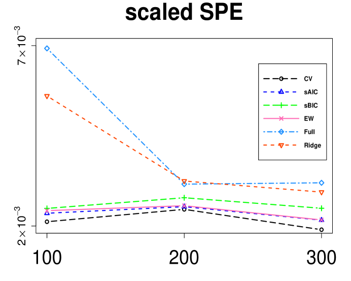
Figure 1: The scaled SPEs by various methods in the intracerebral hemorrhage data analysis for training sample size $n_{\text{train}}=100,200,300$,respectively.

Figure 1 presents the scaled SPEs for model averaging and model selection methods with training size $n_{\text{train}}=100,200,300$, respectively. For ease of presentation, we only exhibit the results without AIC and BIC, as these two approaches have very poor performance. The results show that our estimator frequently produces the most accurate prediction under all circumstances and generally enjoys the smallest scaled SPE among all estimators considered. The above numerical evidence justifies the effectiveness of our method.

VI Concluding Remark

In recent years, as data types are becoming more complex, attention has turned to regression in more abstract settings, such as probability density function, networks, manifolds and simplex-valued responses. However, similar to traditional regression setting, model uncertainty in these abstract settings is still inevitable. The results of singly model selection approach are unstable and might miss some useful information contained in other models. Moreover, in real-world problems, the main focus of applications of various regression is often on prediction rather than solely on the relationships between responses and predictors. Therefore, it becomes crucial to address model uncertainty more properly in the abstract regression framework to make more reliable predictions.

We propose a model averaging procedure to improve prediction for Fréchet regression model where density curves appear as response objects. A weight choice criterion based on minimizing Wasserstein distance of the model average estimator is developed, and the asymptotic optimality of the resultant estimator and consistency of weights are established. Additionally, simulations and real data analysis confirm that our proposed approach outperforms other competitive methods in prediction accuracy. Although the proposed modelling strategy and the resulting predictions are partially stimulated by a particular dataset, apparently, they are widely applicable for other density response datasets from many other disciplines. In the future research, we will extend the proposed averaging method to high-dimensional Fréchet regression, as well as other general types of responses as mentioned above. Understanding the asymptotic results when the sample size is limited and developing finite sample properties are also very necessary in the future research.

Disclosure statement

No potential conflict of interest was reported by the author(s).

Appendix

Proof of Theorem 1. First of all, we notice that

$$\begin{aligned} &\frac{r(\widehat{{\bf w}})}{\inf_{{\bf w}\in\cal{W}}r({\bf w})}-1\\ =&\sup_{{\bf w}\in\cal{W}}\left\{\frac{r(\widehat{{\bf w}})}{r({\bf w})}-1\right\}\\ =&\sup_{{\bf w}\in\cal{W}}\left\{\frac{r(\widehat{{\bf w}})}{R(\widehat{{\bf w}})}\frac{R(\widehat{{\bf w}})}{\bar{R}(\widehat{{\bf w}})}\frac{\bar{R}(\widehat{{\bf w}})}{\bar{R}({\bf w})}\frac{\bar{R}({\bf w})}{R({\bf w})}\frac{R({\bf w})}{r({\bf w})}-1\right\}\\ \leq&\sup_{{\bf w}\in\cal{W}}\frac{r({\bf w})}{R({\bf w})}\sup_{{\bf w}\in\cal{W}}\frac{R({\bf w})}{\bar{R}({\bf w})}\sup_{{\bf w}\in\cal{W}}\frac{\bar{R}(\widehat{{\bf w}})}{\bar{R}({\bf w})}\sup_{{\bf w}\in\cal{W}}\frac{\bar{R}({\bf w})}{R({\bf w})}\sup_{{\bf w}\in\cal{W}}\frac{R({\bf w})}{r({\bf w})}-1\\ =&\sup_{{\bf w}\in\cal{W}}\frac{r({\bf w})}{R({\bf w})}\sup_{{\bf w}\in\cal{W}}\frac{R({\bf w})}{\bar{R}({\bf w})}\frac{\bar{R}(\widehat{{\bf w}})}{\inf_{{\bf w}\in\cal{W}}\bar{R}({\bf w})}\sup_{{\bf w}\in\cal{W}}\frac{\bar{R}({\bf w})}{R({\bf w})}\sup_{{\bf w}\in\cal{W}}\frac{R({\bf w})}{r({\bf w})}-1.\end{aligned}$$

Hence, to prove the Theorem 1, it suffices to show that, as $n\rightarrow\infty$,

$$\sup_{{\bf w}\in{\cal W}}\left|\frac{r({\bf w})}{R({\bf w})}-1\right| \overset{\rm p}{\rightarrow} 0$$ (A.1)

$$\frac{\bar{R}(\widehat{{\bf w}})}{\inf_{{\bf w}\in\cal{W}}\bar{R}({\bf w})} \overset{\rm p}{\rightarrow} 1,$$ (A.2)

and

$$\sup_{{\bf w}\in\cal{W}}\left|\frac{\bar{R}({\bf w})}{R({\bf w})}-1\right| \overset{\rm p}{\rightarrow} 0.$$ (A.3)

We now prove the above equations separately as follows. We first note that

$$R({\bf w}) = \mathbb{E}\frac{1}{n}\sum_{i=1}^{n}d_{W}^{2}\{m_{\oplus}({\bf x}_{i}),\widehat{m}_{\oplus,i}^{[-i]}({\bf w})\}$$

$$= \mathbb{E}\frac{1}{n}\sum_{i=1}^{n}\int_{0}^{1}\left\{Q_{\oplus}({\bf x}_{i},t)-\widehat{Q}_{\oplus,i}^{[-i]}({\bf w},t)\right\}^{2}dt$$

$$= \mathbb{E}\int_{0}^{1}\left\{Q_{\oplus}({\bf x}_{0},t)-\widehat{Q}_{\oplus,0}^{[-1]}({\bf w},t)\right\}^{2}dt$$

$$= \mathbb{E}\int_{0}^{1}\left\{Q_{\oplus}({\bf x}_{0},t)-\widehat{Q}_{\oplus,0}({\bf w},t)\right\}^{2}dt+\mathbb{E}\int_{0}^{1}\left\{\widehat{Q}_{\oplus,0}({\bf w},t)-\widehat{Q}_{\oplus,0}^{[-1]}({\bf w},t)\right\}^{2}dt$$

$$+2\mathbb{E}\left[\int_{0}^{1}\left\{Q_{\oplus}({\bf x}_{0},t)-\widehat{Q}_{\oplus,0}({\bf w},t)\right\}\left\{\widehat{Q}_{\oplus,0}({\bf w},t)-\widehat{Q}_{\oplus,0}^{[-1]}({\bf w},t)\right\}dt\right]$$

$$= r({\bf w})+\mathbb{E}\int_{0}^{1}\left[\sum_{s=1}^{S}w_{s}\left\{\widehat{Q}_{\oplus}({\bf x}_{0}^{(s)},t)-\widehat{Q}_{\oplus}^{[-1]}({\bf x}_{0}^{(s)},t)\right\}\right]^{2}dt$$

$$+2\mathbb{E}\left(\int_{0}^{1}\left\{Q_{\oplus}({\bf x}_{0},t)-\widehat{Q}_{\oplus,0}({\bf w},t)\right\}\left[\sum_{s=1}^{S}w_{s}\left\{\widehat{Q}_{\oplus}({\bf x}_{0}^{(s)},t)-\widehat{Q}_{\oplus}^{[-1]}({\bf x}_{0}^{(s)},t)\right\}\right]dt\right)$$

$$= r({\bf w})+o_{p}(1),$$

uniformly for ${\bf w}\in{\cal W}$, where the last equality is due to the Assumption 2 and Assumption 4. This implies (A.1).

We next deal with equation (A.2). Let

$$\text{CV}_{K}^{\ast}({\bf w}) = \text{CV}_{K}({\bf w})-\sum_{i=1}^{n}d_{W}^{2}(m_{\oplus}({\bf x}_{i}),Y_{i})$$

$$= \text{CV}_{K}({\bf w})-\sum_{i=1}^{n}\int_{0}^{1}\left\{Q_{\oplus}({\bf x}_{i},t)-Y_{i}^{-1}(t)\right\}^{2}dt,$$

where the second term of right hand side of above equation is unrelated to ${\bf w}$. Therefore,

$$\widehat{\bf w} = \underset{{\bf w}\in\cal{W}}{\arg\min}~{}\text{CV}_{K}({\bf w})=\underset{{\bf w}\in\cal{W}}{\arg\min}~{}\text{CV}_{K}^{\ast}({\bf w}).$$

Write

$$\text{CV}_{K}^{\ast}({\bf w}) = n\bar{R}({\bf w})+a_{1}({\bf w})+a_{2}({\bf w}),$$

where $a_{1}({\bf w})=\text{CV}_{K}^{\ast}({\bf w})-nR^{\ast}({\bf w})$ and $a_{2}({\bf w})=nR^{\ast}({\bf w})-n\bar{R}({\bf w})$. By the proof of Theorem $1$ of Wan et al. (2010), if we can show that

$$\sup_{{\bf w}\in\cal{W}}\frac{\left|a_{2}({\bf w})\right|}{nR^{\ast}({\bf w})} = o_{p}(1),$$ (A.4)

and

$$\sup_{{\bf w}\in\cal{W}}\frac{\left|a_{1}({\bf w})\right|}{nR^{\ast}({\bf w})} = o_{p}(1),$$ (A.5)

then (A.2) can be established. So, we next prove the equation (A.4). Recall that $\xi_{n}=n\inf_{w\in\cal W}R^{\ast}({\bf w})$, and notice that

$$\sup_{{\bf w}\in{\cal W}}\frac{\left|a_{2}({\bf w})\right|}{nR^{\ast}({\bf w})}$$ (A.6)

$$\leq \xi_{n}^{-1}\sup_{{\bf w}\in{\cal W}}\left|a_{2}({\bf w})\right|$$

$$= \xi_{n}^{-1}\sup_{{\bf w}\in{\cal W}}\left|nR^{\ast}({\bf w})-n\bar{R}({\bf w})\right|$$

$$= \xi_{n}^{-1}\sup_{{\bf w}\in{\cal W}}\left|\sum_{i=1}^{n}\int_{0}^{1}\left\{Q_{\oplus}({\bf x}_{i},t)-Q^{\ast}_{\oplus,i}({\bf w},t)\right\}^{2}dt-\mathbb{E}\sum_{i=1}^{n}\int_{0}^{1}\left\{Q_{\oplus}({\bf x}_{i},t)-\widehat{Q}_{\oplus,i}({\bf w},t)\right\}^{2}dt\right|$$

$$= \xi_{n}^{-1}\sup_{{\bf w}\in{\cal W}}\left|\sum_{i=1}^{n}\int_{0}^{1}\left\{Q_{\oplus}({\bf x}_{i},t)-Q^{\ast}_{\oplus,i}({\bf w},t)\right\}^{2}dt-\mathbb{E}\sum_{i=1}^{n}\int_{0}^{1}\left\{Q_{\oplus}({\bf x}_{i},t)-Q^{\ast}_{\oplus,i}({\bf w},t)\right\}^{2}dt\right.$$

$$\left.+\mathbb{E}\sum_{i=1}^{n}\int_{0}^{1}\left\{Q_{\oplus}({\bf x}_{i},t)-Q^{\ast}_{\oplus,i}({\bf w},t)\right\}^{2}dt-\mathbb{E}\sum_{i=1}^{n}\int_{0}^{1}\left\{Q_{\oplus}({\bf x}_{i},t)-\widehat{Q}_{\oplus,i}({\bf w},t)\right\}^{2}dt\right|$$

$$\leq \xi_{n}^{-1}\sup_{{\bf w}\in{\cal W}}\left|\mathbb{E}\sum_{i=1}^{n}\int_{0}^{1}\left[\left\{Q_{\oplus}({\bf x}_{i},t)-Q^{\ast}_{\oplus,i}({\bf w},t)\right\}^{2}-\left\{Q_{\oplus}({\bf x}_{i},t)-\widehat{Q}_{\oplus,i}({\bf w},t)\right\}^{2}\right]dt\right|$$

$$+\xi_{n}^{-1}\sup_{{\bf w}\in{\cal W}}\left|\sum_{i=1}^{n}\left(\int_{0}^{1}\left\{Q_{\oplus}({\bf x}_{i},t)-Q^{\ast}_{\oplus,i}({\bf w},t)\right\}^{2}dt\right.\right.$$

$$\left.\left.\ \ -\mathbb{E}\int_{0}^{1}\left\{Q_{\oplus}({\bf x}_{i},t)-m^{\ast}_{\oplus,i}({\bf w},t)\right\}^{2}dt\right)\right|$$

$$\equiv \mathcal{A}_{1n}+\mathcal{A}_{2n}.$$

For the first term of (A.6), we note that

$$\mathbb{E}\sum_{i=1}^{n}\int_{0}^{1}\left[\left\{Q_{\oplus}({\bf x}_{i},t)-Q^{\ast}_{\oplus,i}({\bf w},t)\right\}^{2}-\left\{Q_{\oplus}({\bf x}_{i},t)-\widehat{Q}_{\oplus,i}({\bf w},t)\right\}^{2}\right]dt$$

$$= \mathbb{E}\sum_{i=1}^{n}\int_{0}^{1}\left[\left\{\widehat{Q}_{\oplus}({\bf w},t)-Q_{\oplus}^{\ast}({\bf w},t)\right\}\left\{\widehat{Q}_{\oplus}({\bf w},t)+Q_{\oplus}^{\ast}({\bf w},t)-2Q_{\oplus}({\bf x},t)\right\}\right]dt$$

$$= \mathbb{E}\sum_{i=1}^{n}\int_{0}^{1}\Big{[}-2Q_{\oplus}({\bf x},t)\left\{\widehat{Q}_{\oplus}({\bf w},t)-Q_{\oplus}^{\ast}({\bf w},t)\right\}$$

$$+\left\{\widehat{Q}_{\oplus}({\bf w},t)-Q_{\oplus}^{\ast}({\bf w},t)\right\}\left\{\widehat{Q}_{\oplus}({\bf w},t)+Q_{\oplus}^{\ast}({\bf w},t)\right\}\Big{]}dt$$

$$= \mathbb{E}\sum_{i=1}^{n}\int_{0}^{1}\Big{[}-2Q_{\oplus}({\bf x},t)\left\{\widehat{Q}_{\oplus}({\bf w},t)-Q_{\oplus}^{\ast}({\bf w},t)\right\}$$

$$+\left\{\widehat{Q}_{\oplus}({\bf w},t)-Q_{\oplus}^{\ast}({\bf w},t)\right\}^{2}+2Q_{\oplus}^{\ast}({\bf w},t)\left\{\widehat{Q}_{\oplus}({\bf w},t)-Q_{\oplus}^{\ast}({\bf w},t)\right\}\Big{]}dt$$

$$= O(nc_{n}),$$

where the last equality is due to the Assumption 1 and 2. This leads to $\mathcal{A}_{1n}=O_{p}(\xi_{n}^{-1}nc_{n})=o_{p}(1)$. For the second term of (A.6), we have

$$\sup_{{\bf w}\in{\cal W}}\left|\sum_{i=1}^{n}\left(\int_{0}^{1}\left\{Q_{\oplus}({\bf x}_{i},t)-Q^{\ast}_{\oplus,i}({\bf w},t)\right\}^{2}dt-\mathbb{E}\int_{0}^{1}\left\{Q_{\oplus}({\bf x}_{i},t)-Q^{\ast}_{\oplus,i}({\bf w},t)\right\}^{2}dt\right)\right|$$

$$= \sup_{{\bf w}\in{\cal W}}\left|\sum_{i=1}^{n}\int_{0}^{1}\left\{Q_{\oplus}({\bf x}_{i},t)-\sum_{s=1}^{S}w_{s}Q_{\oplus}^{\ast}({\bf x}_{i}^{(s)},t)\right\}^{2}dt\right.$$

$$\left.\ \ -\mathbb{E}\sum_{i=1}^{n}\left[\int_{0}^{1}\left\{Q_{\oplus}({\bf x}_{i},t)-\sum_{s=1}^{S}w_{s}Q_{\oplus}^{\ast}({\bf x}_{i}^{(s)},t)\right\}^{2}dt\right]\right|$$

$$= \sup_{{\bf w}\in{\cal W}}\left|\sum_{i=1}^{n}\int_{0}^{1}\left[\sum_{s=1}^{S}w_{s}\left\{Q_{\oplus}({\bf x}_{i},t)-m_{\oplus}^{\ast}({\bf x}_{i}^{(s)},t)\right\}\right]^{2}dt\right.$$

$$\left.\ \ -\mathbb{E}\sum_{i=1}^{n}\left(\int_{0}^{1}\left[\sum_{s=1}^{S}w_{s}\left\{Q_{\oplus}({\bf x}_{i},t)-Q_{\oplus}^{\ast}({\bf x}_{i}^{(s)},t)\right\}\right]^{2}dt\right)\right|$$

$$= \sup_{{\bf w}\in{\cal W}}\left|\sum_{i=1}^{n}\int_{0}^{1}\left[\sum_{s_{1}=1}^{S}\sum_{s_{2}=1}^{S}w_{s_{1}}w_{s_{2}}\left\{Q_{\oplus}({\bf x}_{i},t)-Q_{\oplus}^{\ast}({\bf x}_{i}^{(s_{1})},t)\right\}\left\{Q_{\oplus}({\bf x}_{i},t)-Q_{\oplus}^{\ast}({\bf x}_{i}^{(s_{2})},t)\right\}\right]dt\right.$$

$$\left.\ \ -\mathbb{E}\sum_{i=1}^{n}\left\{\int_{0}^{1}\left[\sum_{s_{1}=1}^{S}\sum_{s_{2}=1}^{S}w_{s_{1}}w_{s_{2}}\left\{Q_{\oplus}({\bf x}_{i},t)-Q_{\oplus}^{\ast}({\bf x}_{i}^{(s_{1})},t)\right\}\left\{Q_{\oplus}({\bf x}_{i},t)-Q_{\oplus}^{\ast}({\bf x}_{i}^{(s_{2})},t)\right\}\right]dt\right\}\right|$$

$$\leq \sum_{s_{1}=1}^{S}\sum_{s_{2}=1}^{S}\left|\sum_{i=1}^{n}\left[\int_{0}^{1}\left\{Q_{\oplus}({\bf x}_{i},t)-Q_{\oplus}^{\ast}({\bf x}_{i}^{(s_{1})},t)\right\}\left\{Q_{\oplus}({\bf x}_{i},t)-Q_{\oplus}^{\ast}({\bf x}_{i}^{(s_{2})},t)\right\}dt\right.\right.$$

$$\left.\left.\ \ -\mathbb{E}\int_{0}^{1}\left\{Q_{\oplus}({\bf x}_{i},t)-Q_{\oplus}^{\ast}({\bf x}_{i}^{(s_{1})},t)\right\}\left\{Q_{\oplus}({\bf x}_{i},t)-Q_{\oplus}^{\ast}({\bf x}_{i}^{(s_{2})},t)\right\}dt\right]\right|$$

$$= O_{p}(n^{1/2}S^{2}),$$

where the last step is because the $\mathcal{L}^{2}$-Wasserstein space is equivalent to the subset of $\mathcal{L}^{2}[0,1]$ formed by quantile function on $[0,1]$, and then the central limit theorem can be applied. By the Assumption 3, we have $\mathcal{A}_{2n}=o_{p}(1)$. By above results and (A.6), we conclude that (A.4) holds.

Below we show (A.5). We observe that

$$a_{1}({\bf w})$$

$$= \text{CV}_{K}^{\ast}({\bf w})-nR^{\ast}({\bf w})$$

$$= \sum_{k=1}^{K}\sum_{j=1}^{J}d_{W}^{2}\left\{Y_{(k-1)J+j},\widehat{m}_{\oplus,(k-1)J+j}^{[-k]}({\bf w})\right\}-\sum_{i=1}^{n}\int_{0}^{1}\left\{Q_{\oplus}({\bf x}_{i},t)-Y_{i}^{-1}(t)\right\}^{2}dt$$

$$-\sum_{i=1}^{n}\int_{0}^{1}\left\{Q_{\oplus}({\bf x}_{i},t)-Q^{\ast}_{\oplus,i}({\bf w},t)\right\}^{2}dt$$

$$= \sum_{k=1}^{K}\sum_{j=1}^{J}\int_{0}^{1}\left\{Y_{(k-1)J+j}^{-1}(t)-\widehat{m}_{\oplus,(k-1)J+j}^{[-k]}({\bf w},t)\right\}^{2}dt-\sum_{i=1}^{n}\int_{0}^{1}\left\{Q_{\oplus}({\bf x}_{i},t)-Y_{i}^{-1}(t)\right\}^{2}dt$$

$$-\sum_{i=1}^{n}\int_{0}^{1}\left\{Q_{\oplus}({\bf x}_{i},t)-Q^{\ast}_{\oplus,i}({\bf w},t)\right\}^{2}dt$$

$$= \sum_{k=1}^{K}\sum_{j=1}^{J}\int_{0}^{1}\left[\left\{Y_{(k-1)J+j}^{-1}(t)-Q_{\oplus,(k-1)J+j}({\bf x},t)\right\}+\left\{Q_{\oplus,(k-1)J+j}({\bf x},t)-Q_{\oplus,(k-1)J+j}^{\ast}({\bf w},t)\right\}\right.$$

$$\left.+\left\{Q_{\oplus,(k-1)J+j}^{\ast}({\bf w},t)-\widehat{Q}_{\oplus,(k-1)J+j}({\bf w},t)\right\}+\left\{\widehat{Q}_{\oplus,(k-1)J+j}({\bf w},t)-\widehat{Q}_{\oplus,(k-1)J+j}^{[-k]}({\bf w},t)\right\}\right]^{2}dt$$

$$-\sum_{i=1}^{n}\int_{0}^{1}\left\{Q_{\oplus}({\bf x}_{i},t)-Y_{i}^{-1}(t)\right\}^{2}dt-\sum_{i=1}^{n}\int_{0}^{1}\left\{Q_{\oplus}({\bf x}_{i},t)-Q^{\ast}_{\oplus,i}({\bf w},t)\right\}^{2}dt$$

$$= \sum_{k=1}^{K}\sum_{j=1}^{J}\int_{0}^{1}\left\{\widehat{Q}_{\oplus,(k-1)J+j}({\bf w},t)-\widehat{Q}_{\oplus,(k-1)J+j}^{[-k]}({\bf w},t)\right\}^{2}dt$$

$$+2\sum_{k=1}^{K}\sum_{j=1}^{J}\int_{0}^{1}\left\{Y_{(k-1)J+j}^{-1}(t)-\widehat{Q}_{\oplus,(k-1)J+j}({\bf w},t)\right\}\left\{\widehat{Q}_{\oplus,(k-1)J+j}({\bf w},t)-\widehat{Q}_{\oplus,(k-1)J+j}^{[-k]}({\bf w},t)\right\}dt$$

$$+2\sum_{k=1}^{K}\sum_{j=1}^{J}\int_{0}^{1}\left\{Y_{(k-1)J+j}^{-1}(t)-Q_{\oplus,(k-1)J+j}({\bf w},t)\right\}\left\{Q_{\oplus,(k-1)J+j}({\bf x},t)-Q_{\oplus,(k-1)J+j}^{\ast}({\bf w},t)\right\}dt$$

$$+2\sum_{k=1}^{K}\sum_{j=1}^{J}\int_{0}^{1}\left\{Y_{(k-1)J+j}^{-1}(t)-Q_{\oplus,(k-1)J+j}({\bf w},t)\right\}\left\{Q_{\oplus,(k-1)J+j}^{\ast}({\bf w},t)-\widehat{Q}_{\oplus,(k-1)J+j}({\bf w},t)\right\}dt$$

$$+2\sum_{k=1}^{K}\sum_{j=1}^{J}\int_{0}^{1}\left\{Q_{\oplus,(k-1)J+j}({\bf x},t)-Q_{\oplus,(k-1)J+j}^{\ast}({\bf w},t)\right\}$$

$$\ \ \times\left\{Q_{\oplus,(k-1)J+j}^{\ast}({\bf w},t)-\widehat{Q}_{\oplus,(k-1)J+j}({\bf w},t)\right\}dt$$

$$+\sum_{k=1}^{K}\sum_{j=1}^{J}\int_{0}^{1}\left\{Q_{\oplus,(k-1)J+j}^{\ast}({\bf w},t)-\widehat{Q}_{\oplus,(k-1)J+j}({\bf w},t)\right\}^{2}dt$$

$$+\left[\sum_{k=1}^{K}\sum_{j=1}^{J}\int_{0}^{1}\left\{Y_{(k-1)J+j}^{-1}(t)-Q_{\oplus,(k-1)J+j}({\bf x},t)\right\}^{2}dt-\sum_{i=1}^{n}\int_{0}^{1}\left\{Q_{\oplus}({\bf x}_{i},t)-Y_{i}^{-1}(t)\right\}^{2}dt\right]$$

$$+\left[\sum_{k=1}^{K}\sum_{j=1}^{J}\int_{0}^{1}\left\{Q_{\oplus,(k-1)J+j}({\bf x},t)-Q_{\oplus,(k-1)J+j}^{\ast}({\bf w},t)\right\}dt\right.$$

$$\left.\ \ -\sum_{i=1}^{n}\int_{0}^{1}\left\{Q_{\oplus}({\bf x}_{i},t)-Q^{\ast}_{\oplus,i}({\bf w},t)\right\}^{2}dt\right]$$

$$= \mathcal{B}_{1n}+\mathcal{B}_{2n},$$

where

$$\mathcal{B}_{1n} = \sum_{k=1}^{K}\sum_{j=1}^{J}\int_{0}^{1}\left\{\widehat{Q}_{\oplus,(k-1)J+j}({\bf w},t)-\widehat{Q}_{\oplus,(k-1)J+j}^{[-k]}({\bf w},t)\right\}^{2}dt$$

$$+2\sum_{k=1}^{K}\sum_{j=1}^{J}\int_{0}^{1}\left\{Y_{(k-1)J+j}^{-1}(t)-\widehat{Q}_{\oplus,(k-1)J+j}({\bf w},t)\right\}$$

$$\ \ \times\left\{\widehat{Q}_{\oplus,(k-1)J+j}({\bf w},t)-\widehat{Q}_{\oplus,(k-1)J+j}^{[-k]}({\bf w},t)\right\}dt,$$

and

$$\mathcal{B}_{2n} = 2\sum_{i=1}^{n}\int_{0}^{1}\left\{Y_{i}^{-1}(t)-Q_{\oplus,i}({\bf w},t)\right\}\left\{Q_{\oplus}({\bf x}_{i},t)-Q_{\oplus,i}^{\ast}({\bf w},t)\right\}dt$$

$$+2\sum_{i=1}^{n}\int_{0}^{1}\left\{Y_{i}^{-1}(t)-Q_{\oplus,i}({\bf w},t)\right\}\left\{Q_{\oplus,i}^{\ast}({\bf w},t)-\widehat{Q}_{\oplus,i}({\bf w},t)\right\}dt$$

$$+2\sum_{i=1}^{n}\int_{0}^{1}\left\{Q_{\oplus}({\bf x}_{i},t)-Q_{\oplus,i}^{\ast}({\bf w},t)\right\}\left\{Q_{\oplus,i}^{\ast}({\bf w},t)-\widehat{Q}_{\oplus,i}({\bf w},t)\right\}dt$$

$$+\sum_{i=1}^{n}\int_{0}^{1}\left\{Q_{\oplus,i}^{\ast}({\bf w},t)-\widehat{Q}_{\oplus,i}({\bf w},t)\right\}^{2}dt.$$

For $\mathcal{B}_{2n}$, by the central limit theorem and Assumptions 1 and 2 with $Q_{\oplus}({\bf x}_{i},t)-Q_{\oplus,i}^{\ast}({\bf w},t)=O_{p}(1)$, it is seen that

$$\mathcal{B}_{2n} = O_{p}(n^{1/2})+O_{p}(nc_{n})+O_{p}(nc_{n}^{2})$$ (A.7)

$$= O_{p}(n^{1/2})+O_{p}(nc_{n}).$$

For $\mathcal{B}_{1n}$, we have

$$\mathcal{B}_{1n}$$

$$= \sum_{k=1}^{K}\sum_{j=1}^{J}\int_{0}^{1}\left\{\widehat{Q}_{\oplus,(k-1)J+j}({\bf w},t)-\widehat{Q}_{\oplus,(k-1)J+j}^{[-k]}({\bf w},t)\right\}^{2}dt$$

$$+2\sum_{k=1}^{K}\sum_{j=1}^{J}\int_{0}^{1}\left\{Y_{(k-1)J+j}^{-1}(t)-Q_{\oplus,(k-1)J+j}^{\ast}({\bf w},t)+Q_{\oplus,(k-1)J+j}^{\ast}({\bf w},t)-\widehat{Q}_{\oplus,(k-1)J+j}({\bf w},t)\right\}$$

$$\ \ \ \times\left\{\widehat{Q}_{\oplus,(k-1)J+j}({\bf w},t)-\widehat{Q}_{\oplus,(k-1)J+j}^{[-k]}({\bf w},t)\right\}dt$$

$$= \sum_{k=1}^{K}\sum_{j=1}^{J}\int_{0}^{1}\left\{\widehat{Q}_{\oplus,(k-1)J+j}({\bf w},t)-\widehat{Q}_{\oplus,(k-1)J+j}^{[-k]}({\bf w},t)\right\}^{2}dt$$

$$+2\sum_{k=1}^{K}\sum_{j=1}^{J}\int_{0}^{1}\left\{Y_{(k-1)J+j}^{-1}(t)-Q_{\oplus,(k-1)J+j}^{\ast}({\bf w},t)\right\}\left\{\widehat{Q}_{\oplus,(k-1)J+j}({\bf w},t)-\widehat{Q}_{\oplus,(k-1)J+j}^{[-k]}({\bf w},t)\right\}dt$$

$$+2\sum_{k=1}^{K}\sum_{j=1}^{J}\int_{0}^{1}\left\{Q_{\oplus,(k-1)J+j}^{\ast}({\bf w},t)-\widehat{Q}_{\oplus,(k-1)J+j}({\bf w},t)\right\}$$

$$\ \ \times\left\{\widehat{Q}_{\oplus,(k-1)J+j}({\bf w},t)-\widehat{Q}_{\oplus,(k-1)J+j}^{[-k]}({\bf w},t)\right\}dt$$

$$\leq \sum_{k=1}^{K}\sum_{j=1}^{J}\int_{0}^{1}\left\{\widehat{Q}_{\oplus,(k-1)J+j}({\bf w},t)-\widehat{Q}_{\oplus,(k-1)J+j}^{[-k]}({\bf w},t)\right\}^{2}dt$$

$$+2\sum_{k=1}^{K}\sum_{j=1}^{J}\int_{0}^{1}\left\{Y_{(k-1)J+j}^{-1}(t)-Q_{\oplus,(k-1)J+j}^{\ast}({\bf w},t)\right\}\left\{\widehat{Q}_{\oplus,(k-1)J+j}({\bf w},t)-\widehat{Q}_{\oplus,(k-1)J+j}^{[-k]}({\bf w},t)\right\}dt$$

$$+\sum_{k=1}^{K}\sum_{j=1}^{J}\int_{0}^{1}\left\{Q_{\oplus,(k-1)J+j}^{\ast}({\bf w},t)-\widehat{Q}_{\oplus,(k-1)J+j}({\bf w},t)\right\}^{2}dt$$

$$+\sum_{k=1}^{K}\sum_{j=1}^{J}\int_{0}^{1}\left\{\widehat{Q}_{\oplus,(k-1)J+j}({\bf w},t)-\widehat{Q}_{\oplus,(k-1)J+j}^{[-k]}({\bf w},t)\right\}^{2}dt.$$

Note that from the formula of (11) and Assumption 2, we have $n^{-1}\xi_{n}=O_{p}(1)$, and combining with Assumption 4, we obtain

$$\left\{\widehat{Q}_{\oplus,(k-1)J+j}({\bf w},t)-\widehat{Q}_{\oplus,(k-1)J+j}^{[-k]}({\bf w},t)\right\}^{2}$$

$$= \left[\sum_{s=1}^{S}w_{s}\left\{\widehat{Q}_{\oplus}({\bf x}_{(k-1)J+j}^{(s)},t)-\widehat{Q}_{\oplus}^{[-k]}({\bf x}_{(k-1)J+j}^{(s)},t)\right\}\right]^{2}$$

$$= o_{p}(n^{-1}\xi_{n})$$

$$= o_{p}(1).$$

Based on above result and Assumption 4, we have

$$\mathcal{B}_{1n} = o_{p}(\xi_{n})+o_{p}(\xi_{n})+O_{p}(nc_{n}^{2})+o_{p}(\xi_{n})$$ (A.8)

$$= o_{p}(\xi_{n})+O_{p}(nc_{n}^{2}).$$

Therefore, by (A.7) and (A.8), we have $a_{1}({\bf w})=O_{p}(n^{1/2})+O_{p}(nc_{n})+o_{p}(\xi_{n}).$ Based on $R^{\ast}({\bf w})=O_{p}(1)$ deduced from Assumption 2, we can see that (A.5) holds. This completes the proof of (A.2).

For (A.3), by the proof of (A.6), it follows that

$$n\bar{R}({\bf w})-nR({\bf w}) = n\bar{R}({\bf w})-nR^{\ast}(w)+nR^{\ast}(w)-nR({\bf w})$$

$$= nR^{\ast}(w)-nR({\bf w})+O_{p}(nc_{n})+O_{p}(n^{1/2}S^{2}).$$

Note that $\widehat{m}_{\oplus,i}^{[-i]}({\bf w},t)$ is the estimator of $m_{\oplus}({\bf x}_{i},t)$ without using the $i$th observation, so it shares the same limits as $\widehat{m}_{\oplus,i}({\bf w},t)$. Thus, we also have $nR^{\ast}(w)-nR({\bf w})=nO(n^{-1/(2(\beta-1))})+O_{p}(n^{1/2}S^{2})$, which entails that $\bar{R}({\bf w})-R({\bf w})=O_{p}(c_{n})+O_{p}(n^{-1/2}S^{2})=o_{p}(1)$, by Assumption 3. Then, this establishes the (A.3), which completes the proof. ∎

Proof of Theorem 2. For the sake of simplicity in notation, let $\tau=\sum_{s\in\mathcal{C}}w_{s}$ and $\widehat{\tau}=\sum_{s\in\mathcal{C}}\widehat{w}_{s}$. We next to show that $\widehat{\tau}\rightarrow 1$ in probability. Further, let $\bm{\lambda}$ be also a weight vector of $S$ dimension with $\lambda_{s}=0$ for $s\in\mathcal{C}$ and $\lambda_{s}=w_{s}/(1-\tau)$ for $s\notin\mathcal{C}$. From the proof of (A.5), we know that

$$\text{CV}_{K}^{\ast}({\bf w})/n-R^{\ast}({\bf w}) = O_{p}(n^{-1/2})+O_{p}(c_{n})+o_{p}(\xi_{n}/n)$$

$$= O_{p}(n^{-1/2})+O_{p}(c_{n})+o_{p}(1).$$

Note that the above result also holds by replacing weight ${\bf w}$ with $\widehat{\bf w}$. That is,

$$\text{CV}_{K}^{\ast}(\widehat{\bf w})/n-R^{\ast}(\widehat{\bf w}) = O_{p}(n^{-1/2})+O_{p}(c_{n})+o_{p}(1).$$ (A.9)

Note that

$$R^{\ast}({\bf w}) = \frac{1}{n}\sum_{i=1}^{n}d_{W}^{2}\{m_{\oplus}({\bf x}_{i}),m^{\ast}_{\oplus,i}({\bf w})\}$$ (A.10)

$$= \frac{1}{n}\sum_{i=1}^{n}\int_{0}^{1}\left\{Q_{\oplus}({\bf x}_{i},t)-Q^{\ast}_{\oplus,i}({\bf w},t)\right\}^{2}dt$$

$$= \frac{1}{n}\sum_{i=1}^{n}\int_{0}^{1}\left[\sum_{s=1}^{S}w_{s}\left\{Q_{\oplus}({\bf x}_{i},t)-Q_{\oplus}^{\ast}({\bf x}_{i}^{(s)},t)\right\}\right]^{2}dt$$

$$= \frac{1}{n}\sum_{i=1}^{n}\int_{0}^{1}\left[\sum_{s\notin\mathcal{C}}w_{s}\left\{Q_{\oplus}({\bf x}_{i},t)-Q_{\oplus}^{\ast}({\bf x}_{i}^{(s)},t)\right\}\right]^{2}dt$$

$$= (1-\tau)^{2}\frac{1}{n}\sum_{i=1}^{n}\int_{0}^{1}\left[\sum_{s\notin\mathcal{C}}\frac{w_{s}}{1-\tau}\left\{Q_{\oplus}({\bf x}_{i},t)-Q_{\oplus}^{\ast}({\bf x}_{i}^{(s)},t)\right\}\right]^{2}dt$$

$$= (1-\tau)^{2}\frac{1}{n}\sum_{i=1}^{n}\int_{0}^{1}\left[\sum_{s=1}^{S}\lambda_{s}\left\{Q_{\oplus}({\bf x}_{i},t)-Q_{\oplus}^{\ast}({\bf x}_{i}^{(s)},t)\right\}\right]^{2}dt$$

$$= (1-\tau)^{2}R^{\ast}(\bm{\lambda}).$$

It is also easy to see that the above result holds by replacing weight ${\bf w}$ with $\widehat{\bf w}$, and together with (A.9) and (A.10), we have

$$\text{CV}_{K}^{\ast}(\widehat{\bf w})/n = (1-\widehat{\tau})^{2}R^{\ast}(\widehat{\bm{\lambda}})+O_{p}(n^{-1/2})+O_{p}(c_{n})+o_{p}(1),$$ (A.11)

where $\widehat{\lambda}_{s}=\widehat{w}_{s}/(1-\widehat{\tau})$ when $s\notin\mathcal{C}$ and $\widehat{\lambda}_{s}=0$ when $s\in\mathcal{C}$. Let $\widetilde{\bf w}$ be a weight vector satisfying $\sum_{s\in\mathcal{C}}\widetilde{w}_{s}=1$. For any correctly specified model $s\in\mathcal{C}$, we have $m_{\oplus}({\bf x}_{i},t)-m_{\oplus}^{\ast}({\bf x}_{i}^{(s)},t)=0,$ from which and formula of (A.10), we have $R^{\ast}(\widetilde{\bf w})=0$. Then, it follows that, from (A.9),

$$\text{CV}_{K}^{\ast}(\widetilde{\bf w})/n = O_{p}(n^{-1/2})+O_{p}(c_{n})+o_{p}(1).$$ (A.12)

Recall that the fact $\widehat{\bf w}$ minimizes $\text{CV}_{K}^{\ast}({\bf w})$, and combining (A.11) and (A.12), we have

$$(1-\widehat{\tau})^{2}R^{\ast}(\widehat{\bm{\lambda}})+O_{p}(n^{-1/2})+O_{p}(c_{n})+o_{p}(1) \leq \text{CV}_{K}^{\ast}(\widetilde{\bf w})/n=O_{p}(n^{-1/2})+O_{p}(c_{n})+o_{p}(1),$$

from which, we have

$$(1-\widehat{\tau})^{2}\inf_{{\bf w}\in\cal{W}_{S}}R^{\ast}({\bf w}) \leq O_{p}(n^{-1/2})+O_{p}(c_{n})+o_{p}(1).$$

Thus, based on above result and Assumption 5, we conclude that $\widehat{\tau}\overset{\rm p}{\rightarrow}1$. The proof is completed. ∎

TABLE I: Monte Carlo results for averaged risk. The sample size $n$ equals to $100$, $200$ and $300$, respectively. Standard deviations are given in parentheses. In each setting, the method with the best performance is marked in bold.

$n$	$100$	$200$	$300$
CV	0.0709 (0.0273)	0.0324 (0.0154)	0.0217 (0.0121)
sAIC	0.0756 (0.0249)	0.0381 (0.0170)	0.0244 (0.0119)
sBIC	0.0786 (0.0248)	0.0389 (0.0177)	0.0248 (0.0120)
EW	0.0759 (0.0259)	0.0372 (0.0166)	0.0245 (0.0120)
Oracle	0.0612 (0.0238)	0.0268 (0.0144)	0.0190 (0.0118)
Full	0.1489 (0.0450)	0.0780 (0.0248)	0.0525 (0.0165)
Ridge	0.1114 (0.0361)	0.0525 (0.0200)	0.0337 (0.0163)
AIC	0.1387 (0.0456)	0.0696 (0.0258)	0.0460 (0.0169)
BIC	0.2520 (0.1073)	0.0946 (0.0667)	0.0417 (0.0141)

TABLE II: The sum of weights assigned to correct candidate models.

Scenario		Sum
$n=100$			0.9211
$n=200$			0.9723
$n=300$			0.9939

References

- (1)
- Ando and Li (2014) Ando, T. and Li, K.-C. (2014), ‘A model-averaging approach for high-dimensional regression’, Journal of the American Statistical Association 109(505), 254–265.
- Arlot and Lerasle (2016) Arlot, S. and Lerasle, M. (2016), ‘Choice of V for V-fold cross-validation in least-squares density estimation’, The Journal of Machine Learning Research 17(1), 7256–7305.
- Bates and Granger (1969) Bates, J. M. and Granger, C. W. (1969), ‘The combination of forecasts’, Journal of the operational research society 20(4), 451–468.
- Bigot et al. (2017) Bigot, J., Gouet, R., Klein, T. and López, A. (2017), ‘Geodesic PCA in the Wasserstein space by convex PCA’, Annales de l’Institut Henri Poincaré-Probabilités et Statistiques 53(1), 1–26.
- Buckland et al. (1997) Buckland, S. T., Burnham, K. P. and Augustin, N. H. (1997), ‘Model selection: an integral part of inference’, Biometrics 53(2), 603–618.
- Chen et al. (2021) Chen, Y., Lin, Z. and Müller, H.-G. (2021), ‘Wasserstein regression’, Journal of the American Statistical Association 118(542), 1–14.
- Dubey and Müller (2020) Dubey, P. and Müller, H.-G. (2020), ‘Fréchet change-point detection’, The Annals of Statistics 48(6), 3312–3335.
- Feng et al. (2022) Feng, Y., Liu, Q., Yao, Q. and Zhao, G. (2022), ‘Model averaging for nonlinear regression models’, Journal of Business & Economic Statistics 40(2), 785–798.
- Fréchet (1948) Fréchet, M. (1948), ‘Les éléments aléatoires de nature quelconque dans un espace distancié’, Annales de l’Institut Henri Poincaré 10, 215–310.
- Gao et al. (2016) Gao, Y., Zhang, X., Wang, S. and Zou, G. (2016), ‘Model averaging based on leave-subject-out cross-validation’, Journal of Econometrics 192(1), 139–151.
- Ghodrati and Panaretos (2022) Ghodrati, L. and Panaretos, V. M. (2022), ‘Distribution-on-distribution regression via optimal transport maps’, Biometrika 109(4), 957–974.
- Han et al. (2019) Han, K., Müller, H.-G. and Park, B. U. (2019), ‘Additive functional regression for densities as responses’, Journal of the American Statistical Association 115(530), 997–1010.
- Hansen (2007) Hansen, B. E. (2007), ‘Least squares model averaging’, Econometrica 75(4), 1175–1189.
- Hevesi et al. (2018) Hevesi, M., Bershad, E. M., Jafari, M., Mayer, S. A., Selim, M., Suarez, J. I. and Divani, A. A. (2018), ‘Untreated hypertension as predictor of in-hospital mortality in intracerebral hemorrhage: a multi-center study’, Journal of Critical Care 43, 235–239.
- Hoeting et al. (1999) Hoeting, J. A., Madigan, D., Raftery, A. E. and Volinsky, C. T. (1999), ‘Bayesian model averaging: a tutorial’, Statistical Science 14(4), 382–417.
- Leung and Barron (2006) Leung, G. and Barron, A. R. (2006), ‘Information theory and mixing least-squares regressions’, IEEE Transactions on information theory 52(8), 3396–3410.
- Li et al. (2022) Li, J., Lv, J., Wan, A. T. K. and Liao, J. (2022), ‘Adaboost semiparametric model averaging prediction for multiple categories’, Journal of the American Statistical Association 117(537), 495–509.
- Liang et al. (2011) Liang, H., Zou, G., Wan, A. T. K. and Zhang, X. (2011), ‘Optimal weight choice for frequentist model average estimators’, Journal of the American Statistical Association 106(495), 1053–1066.
- Lin et al. (2023) Lin, Z., Kong, D. and Wang, L. (2023), ‘Causal inference on distribution functions’, Journal of the Royal Statistical Society Series B: Statistical Methodology 85(2), 378–398.
- Liu et al. (2020) Liu, Q., Yao, Q. and Zhao, G. (2020), ‘Model averaging estimation for conditional volatility models with an application to stock market volatility forecast’, Journal of Forecasting 39(5), 841–863.
- Lu and Su (2015) Lu, X. and Su, L. (2015), ‘Jackknife model averaging for quantile regressions’, Journal of Econometrics 188(1), 40–58.
- Panaretos and Zemel (2016) Panaretos, V. M. and Zemel, Y. (2016), ‘Amplitude and phase variation of point processes’, The Annals of Statistics 44(2), 771–812.
- Petersen et al. (2021) Petersen, A., Liu, X. and Divani, A. A. (2021), ‘Wasserstein F-tests and confidence bands for the Fréchet regression of density response curves’, The Annals of Statistics 49(1), 590–611.