Fundamental dynamics of popularity-similarity trajectories in real networks

Abstract

Real networks are complex dynamical systems, evolving over time with the addition and deletion of nodes and links. Currently, there exists no principled mathematical theory for their dynamics—a grand-challenge open problem in complex networks. Here, we show that the popularity and similarity trajectories of nodes in hyperbolic embeddings of different real networks manifest universal self-similar properties with typical Hurst exponents $H\ll 0.5$. This means that the trajectories are anti-persistent or ‘mean-reverting’ with short-term memory, and they can be adequately captured by a fractional Brownian motion process. The observed behavior can be qualitatively reproduced in synthetic networks that possess a latent geometric space, but not in networks that lack such space, suggesting that the observed subdiffusive dynamics are inherently linked to the hidden geometry of real networks. These results set the foundations for rigorous mathematical machinery for describing and predicting real network dynamics.

Modeling and prediction of network dynamics, i.e., of the connections and disconnections that take place in a given network over different time scales, is perhaps the most fundamental unresolved problem in network science Krioukov (2014), listed also in the popular 23 Mathematical Challenges of DARPA DAR (2007). Understanding network dynamics is a key to better prediction and control of the behavior of networks and of the processes running on them, such as epidemic spreading and cascading failure propagation Easley and Kleinberg (2010).

We observe that the mathematical machinery and equations that describe the evolution of other complex dynamical systems and temporal data, such as gravitational and molecular systems, turbulence, and financial data, have been well-developed and known for decades Alder and Wainwright (1959); Aarseth (2003); Schlick (2010); Friedrich et al. (2011); Mandelbrot and Ness (1968). Yet, the underlying processes governing network dynamics and their mathematics remain elusive. One of the main reasons for this discrepancy is the fact that networks are discrete topological structures, not inheriting the standard form of temporal data met in other classical dynamical systems.

Advancements in network geometry during the past years revealed that real networks can be meaningfully mapped (or embedded) into hyperbolic spaces Krioukov et al. (2010); Boguñá et al. (2010); Papadopoulos et al. (2012); García-Pérez et al. (2019); Boguñá et al. (2021). In these spaces, each node $i$ is represented by its radial (popularity) and angular (similarity) coordinates $r_{i},\theta_{i}$, while hyperbolically closer nodes have higher chances of being connected Krioukov et al. (2010). Therefore, if the mathematics describing the evolution of the nodes’ coordinates was known, one could employ this mathematics to describe, and ultimately predict, network dynamics. In essence, we observe that network geometry provides a way of casting the problem of network dynamics to a time series prediction problem—a well-mined problem in other areas, such as finance Mandelbrot and Ness (1968); Mandelbrot et al. (1997); Muniandy and Lim (2001); Friedrich et al. (2011), network traffic modeling Leland et al. (1993); Liu et al. (1999), and fluid dynamics Friedrich and Peinke (1997); Hadjihosseini et al. (2014).

Given these considerations, here we analyze, for the first time, historical popularity and similarity trajectories of nodes in hyperbolic embeddings of different real networks and find that both types of trajectories exhibit subdiffusive dynamics (see Table 1 for the considered data). Specifically, we find that the trajectories are anti-persistent with short-term negative autocorrelations, and can be well described by a fractional Brownian motion process Mandelbrot and Ness (1968).

These findings, and particularly the departure from the traditional law of Brownian motion, are in agreement with intuition. Indeed, real networks are characterized by strong community structures and hierarchical organization that persist over time Dorogovtsev (2010). The first characteristic implies that similarity trajectories should remain confined within specific regions of the similarity space, occupied by the nodes’ clusters or communities. The second characteristic signifies that popularity trajectories should fluctuate around some expected values that reflect the node positions in the network hierarchy or popularity space. For instance, a non-hub node in the US air transportation network is expected to remain a non-hub even though its degree can fluctuate. Further, since the popularity and similarity trajectories are not generally independent, the dynamics of one can influence the dynamics of the other. This picture is analogous to subdiffusive phenomena found in crowded biological systems, where particles diffuse in environments with hierarchies of energy barriers or traps Saxton (2007).

The identified type of dynamics, which is characterized by anti-persistent memory effects, holds particular significance as it favors plausible predictions for the connectivity dynamics of real networks. In contrast, as we show, trajectories obtained from non-geometric synthetic networks, i.e., networks that lack an underlying hyperbolic geometry, do not exhibit the same characteristics. Specifically, in such cases, similarity trajectories resemble traditional Brownian motion (and are thus unpredictable), while anti-persistency in popularity trajectories significantly weakens.

Name	Type	Nodes	Period	No. of snapshots	Source
US Air	Transportation	US airports	1988-2015	10000 (daily)	USA
Bitcoin (BTC)	Financial	Bitcoin addresses	2012-2016	1292 (daily)	Kosyfaki and Mamoulis (2022); btc
PGP WoT	Trust	PGP certificates	2003-2007	1500 (daily)	pgp
IPv6 Internet	Technological	Autonomous systems	2011-2017	300 (weekly)	as_
arXiv	Collaboration	Authors	2011-2022	3977 (daily)	arx

Table 1: Overview of the considered real-world network data. Details for each data set can be found in Appendix A. All data sets along with code will be made available upon publication.

Dynamics of popularity-similarity trajectories in real networks

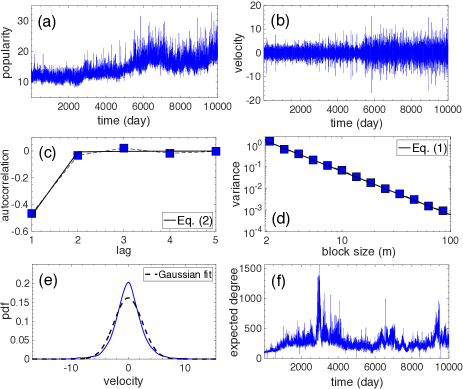
Figure 1: Properties of the popularity trajectory of CLT in the US Air transportation network. (a) Radial popularity trajectory. (b) Trajectory increments (velocity). (c) Sample autocorrelation of the velocity process. The solid line corresponds to Eq. (2). (d) Variance-time plot of the velocity process. The solid line corresponds to Eq. (1). (e) Probability density function (pdf) of the velocity. The dashed curve shows a Gaussian pdf with the same mean and variance. (f) Expected degree trajectory. The estimated Hurst exponents for the trajectories in (a) and (f) are $0.0004$ and $0.02$. Time in the $x$-axis of (a), (b) and (f), is measured in days from the year $1988$ to $2015$.

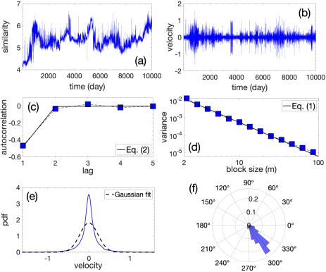
Figure 2: Properties of the similarity trajectory of CLT in the US Air transportation network. (a) Angular similarity trajectory. The $y$-axis is in radians. (b) Trajectory increments (angular velocity). (c)-(e) show the same as (c)-(e) in Fig. 1, but for the similarity trajectory. (f) Angular distribution of the similarity coordinate during the years 1988-2015. The estimated Hurst exponent for the trajectory is $H=0.03$.

Trajectory extraction

For each real network, we consider consecutive snapshots of its topology, $G_{1},G_{2},\ldots,G_{\tau}$, spanning the period shown in Table 1. We independently map each snapshot $G_{t},t=1,\ldots,\tau$, to an underlying hyperbolic space using Mercator García-Pérez et al. (2019) and extract for each node $i$ its popularity and similarity trajectories, i.e., the evolution of its popularity and similarity coordinates, $\{r_{i}(t),\theta_{i}(t)\},t=1,\ldots,\tau$ (see Appendix B). We choose to independently map the snapshots in order to avoid possible artificial biases between node coordinates across embeddings, and apply Procrustean rotations Rohlf and Slice (1990) to eliminate global rotations and reflections (see Appendix C).

We note that for each node $i$ its coordinates $r_{i}(t)$ and $\theta_{i}(t)$ are inferred from the observed network topology at time $t$, $G_{t}$, and represent estimates for some underlying or ‘hidden’ true coordinates that determine network connectivity Boguñá et al. (2010). When $G_{t}$ changes, these estimates also change. Furthermore, for each node $i$ we also consider the trajectory of its expected degree $\kappa_{i}(t)$, which is related to its radial coordinate $r_{i}(t)$ via $r_{i}(t)\sim R(t)-2\ln{\kappa_{i}(t)}$, where $R(t)$ is the radius of the hyperbolic disc where nodes reside García-Pérez et al. (2019). We consider the expected degrees, since unlike radial coordinates, they are not directly linked to the evolution of $R(t)$ and thus provide a more direct view on individual node popularity (see Appendix B for further details).

Figures 1(a) and 2(a) show the popularity and similarity trajectories of the Charlotte Douglas International Airport (CLT) in the US Air transportation network. Figure 1(f) shows the trajectory of CLT’s expected degree (see Appendix H for other examples).

Anti-persistence and self-similarity properties

We find that the obtained trajectories constitute well-defined time series, exhibiting universal properties. Particularly, their velocities (or increments, i.e., differences between consecutive observations) manifest negative autocorrelations with short-term memory (see Figs. 1(b),(c), 2(b),(c), and Appendix E). Furthermore, the velocities exhibit self-similar scale laws of fractional order, i.e., they are of fractal nature (see Figs. 1(d) and 2(d) that are explained below, and Appendix H for more examples).

A way to quantify the self-similarity and the type of memory inherited by the trajectories is by computing their Hurst exponent $H\in(0,1)$ Hurst (1951). For a self-similar time series the Hurst exponent is directly related to its fractal dimension $D=2-H$ Mandelbrot (1985). A value of $H$ in $(0.5,1)$ indicates a persistent or trend-like time series with long-range positive autocorrelation (a superdiffusive process); this means that positive (negative) increments tend to be followed by another positive (negative) increments, and such dependence decays slowly with the time lag between the increments. The strength of persistence increases as $H$ approaches $1$. On the other hand, a value of $H$ in $(0,0.5)$ indicates an anti-persistent or ‘mean-reverting’ time series with negative autocorrelation (a subdiffusive process); in this case, positive (negative) increments tend to be followed by negative (positive) increments, and the dependence between increments is short-ranged. The strength of anti-persistence increases as $H$ approaches $0$. The case $H=0.5$ corresponds to zero autocorrelation, i.e., to a completely random process with no dependence between its increments (typical diffusion).

Figure 3 shows the distribution of Hurst exponents $H$ across the trajectories in the considered networks. To calculate $H$ we use the method of absolute moments Preis et al. (2009); Górski et al. (2002) (see Appendix D). We see that in general the distributions are concentrated over values of $H$ well below $0.5$, indicating that the trajectories are generally strongly anti-persistent. The strongest anti-persistence (lowest average $H$) is observed in the US Air and BTC, for both the popularity and similarity trajectories, followed by PGP, IPv6, and arXiv (see the legend of Fig. 3 for the average $H$ in each case). We note that values of $H$ close to $0$ are not bizarre, but have also been observed in other real-world data Gatheral et al. (2018); Neuman and Rosenbaum (2018). In general, the popularity trajectories are more anti-persistent than the similarity trajectories, while the least anti-persistence is observed in the similarity trajectories of arXiv. For comparison, Fig. 3 shows also the distributions of $H$ in randomized counterparts of the trajectories, obtained by randomizing the sign of the velocities, which breaks the correlations in the trajectories (see Appendix E). As expected, these distributions are concentrated around $H=0.5$.

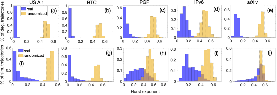
Figure 3: Distribution of Hurst exponents in the considered real networks (in blue). (a) to (e) correspond to the expected degree trajectories. The corresponding average Hurst exponents are $0.01$, $0.02$, $0.05$, $0.13$, and $0.1$. (f) to (j) correspond to the similarity trajectories. The corresponding average Hurst exponents are $0.08$, $0.07$, $0.30$, $0.25$, and $0.46$. The distributions are computed by considering all trajectories with at least $300$ points. The plots also show the distributions for the randomized counterparts of the trajectories (in yellow). Similar results hold for the radial trajectories (see Appendix F).

To further support the above findings, we also construct the variance-time plot Leland et al. (1993). Specifically, let $X_{k}^{(m)}=(X_{km-m+1}+\ldots+X_{km})/m$, $k=1,2,3,\ldots$, denote an aggregated point series of the velocities over non-overlapping blocks of size $m$, where $m$ is a positive integer, $m\geq 2$. If $m^{1-H}X^{(m)}\stackrel{{\scriptstyle d}}{{=}}X$, where $\stackrel{{\scriptstyle d}}{{=}}$ denotes equivalency in finite joint distribution and $X$ is the original non-aggregated series, then $X$ is said to be self-similar with Hurst exponent $H$. Self-similarity implies that the variance of $X^{(m)}$ satisfies

$$\textnormal{Var}(X^{(m)})=\sigma^{2}m^{2H-2},$$ (1)

where $\sigma^{2}$ is the variance of $X$. We find that the variance-time plots of the velocity processes, i.e., the empirical plots of $\log{\textnormal{Var}(X^{(m)})}$ against $\log{m}$, indeed follow closely Eq. (1) with the estimated values of Hurst exponents (see Figs. 1(d) and 2(d), and Appendix H).

Understanding the emergence of anti-persistence

To understand the origin of the observed anti-persistence in the trajectories, we consider a simple network model where snapshots $G_{t}$, $t=1,2,\ldots,\tau$, undergo link rewirings that preserve their statistical characteristics, including their degree distribution and clustering (see Appendix J). In the geometric version of the model, the snapshots are constructed according to random hyperbolic graphs (RHGs) Krioukov et al. (2010). Here the snapshots are built over an underlying similarity space. Nodes in this space are assigned fixed similarity coordinates $\theta_{h}$ and target expected degrees $\kappa_{h}$, referred to as ‘hidden variables’, and are connected with a probability that decreases with their effective distance, $\Delta\theta_{h}/(\kappa_{h}\kappa_{h}^{\prime})$, where $\Delta\theta_{h}$ is the similarity distance and $\kappa_{h},\kappa_{h}^{\prime}$ are the nodes’ expected degrees. In the non-geometric version of the model, the snapshots are constructed either according to the configuration model (CM) Chung and Lu (2002) or to random graphs (RGs) Solomonoff and Rapoport (1951). In CM the connection probability depends only on the nodes’ expected degrees $\kappa_{h}$ and $\kappa_{h}^{\prime}$, while in RGs all nodes have the same expected degree and connected with the same probability. The link-rewiring process involves deleting at random a number of links from snapshot $G_{t}$ and subsequently reinserting an equal number of links to generate the next snapshot $G_{t+1}$, according to the connection probability in the corresponding model (see Appendix J).

Once the snapshots are created, we embed them into hyperbolic spaces and extract the nodes’ expected degree and similarity trajectories, $\kappa(t)$ and $\theta(t)$, following the same procedure as in the real networks. We recall that $\kappa(t)$ and $\theta(t)$ are topology-inferred estimates for the nodes’ underlying coordinates and thus change with the topology $G_{t}$. In RHGs, the underlying coordinates are the nodes’ hidden variables $\kappa_{h}$ and $\theta_{h}$, while in CM and RGs the nodes do not have underlying similarity coordinates $\theta_{h}$, but only popularity coordinates $\kappa_{h}$.

We find that the obtained trajectories in the RHGs model exhibit negative autocorrelations and strong anti-persistence, as indicated by low Hurst exponents, similar to those observed in real networks (see Fig. 4(a),(b), and Figs. 43 and 46). Furthermore, as in real networks, the similarity trajectories tend to be confined within specific regions of the similarity space (see Fig. 4(c),(d), and Fig. 2(a),(f)). In contrast, the similarity trajectories in CM and RGs resemble Brownian motion (or the randomized counterparts of the real trajectories), having Hurst exponents close to $0.5$ and spreading throughout the similarity space (see Fig. 4(b),(e),(f), and Figs. 44 and 45).

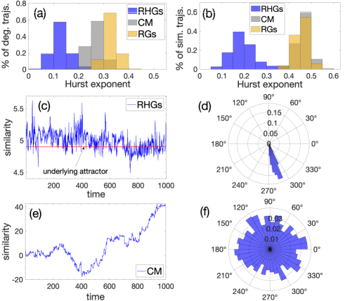
Figure 4: Expected degree and similarity trajectories in synthetic temporal networks constructed according to random hyperbolic graphs (RHGs), the configuration model (CM), and random graphs (RGs). (a) and (b) show the distribution of Hurst exponents for the expected degree and similarity trajectories in the three cases. (c) and (d) show a similarity trajectory in the RHGs model and its distribution in the similarity space. The red line in (c) indicates the underlying attractor, i.e., the node’s hidden similarity coordinate $\theta_{h}=4.9$. (e) and (f) show the same as in (c) and (d), but for the CM case. There is no underlying similarity attractor here. The estimated Hurst exponent for the trajectory in (c) is 0.16, while for the trajectory in (e) is 0.42.

Unlike similarity trajectories, the expected degree trajectories do not lose their anti-persistence in CM and RGs, although this characteristic weakens (see Fig. 4(a) and Figs. 47 and 48). Furthermore, we find that heterogeneous distributions of the hidden degrees $\kappa_{h}$ lead to stronger degree anti-persistence. This is evident from the distributions of Hurst exponents in CM and RGs in Fig. 4(a). In the considered example, the degree distribution in CM is a power law, while in RGs it is Poissonian (see Appendix J).

These results can be intuitively explained as follows. First, consider the RHGs case. Even though the snapshots $G_{t}$, $t=1,2,\ldots$, differ from each other due to link rewirings, they are all created using the same set of underlying node coordinates. Consequently, the inferred coordinates $\kappa(t)$ and $\theta(t)$ for each node should remain close to their respective underlying coordinates $\kappa_{h}$ and $\theta_{h}$ at all times $t$. Further, whenever the inferred coordinates happen to deviate significantly from their underlying coordinates, then in the subsequent time step it is more likely that they will be closer to them; otherwise, the inferred coordinates would eventually diverge from their underlying coordinates. Additionally, the inferred coordinates never settle onto their underlying ones, which means that whenever they are sufficiently close to them, then in the subsequent time step they are likely to drift away due to probabilistic network changes. In essence, the underlying coordinates of a node can be seen as ‘attractors’ that pull the inferred coordinates close to them. These attractors are in competition with connectivity changes that push the inferred coordinates away from them. This competition explains the observed reversal nature of the trajectories, i.e., anti-persistence (cf. Fig. 4(c)).

In CM and RGs, there are no underlying similarity attractors, and thus $\theta(t)$ can change freely, leading to diffusive dynamics (cf. Fig. 4(e),(f)). On the other hand, there are still popularity attractors $\kappa_{h}$, which explains the anti-persistence of the expected degree trajectories. However, this anti-persistence is weaker than in RHGs, as the degree trajectories depend on the similarity trajectories García-Pérez et al. (2019), and the latter are no longer anti-persistent. Further, we observe that the degree trajectories can significantly deviate from their underlying attractors, which is not the case in RHGs (see Figs. 46-48(a)). Finally, when the underlying attractors $\kappa_{h}$ are heterogeneously distributed, tighter constraints are imposed to individual degree trajectories, which supports the stronger degree anti-persistence in CM compared to RGs in Fig. 4(a).

Taken altogether, these results indicate that the observed anti-persistence of the real-world trajectories is inherently linked to the latent geometry of real networks, i.e., to their intrinsic similarity-popularity space Papadopoulos et al. (2012). Community structure in real networks can enhance anti-persistence by further constraining the trajectories. Furthermore, the underlying popularity and similarity attractors do not have to remain fixed as in the RHGs model, but can change over time, reflecting long-term popularity and similarity shifts. Importantly, as explained next, the strong anti-persistence of the real-world trajectories, quantified by their low Hurst exponents, favors plausible predictions for their evolution, and therefore, for the evolution of the underlying attractors that are closely aligned with them.

Modeling with fractional Brownian motion

Fractional Brownian motion (fBm) indexed by a Hurst exponent $H$, $B_{H}(t),t\geq 0$, is a popular stochastic process often used as a basis in the modeling and simulation of real-world time series Mandelbrot and Ness (1968). fBm generalizes Brownian motion (Bm), however, unlike Bm, the increments of fBm need not be independent, although they are still stationary. Specifically, the increment process $X_{H}(t)=B_{H}(t+1)-B_{H}(t)$ is called fractional Gaussian noise (fGn) and has the following autocorrelation function Mandelbrot and Ness (1968):

$$\rho(l)=0.5\left(|l+1|^{2H}-2|l|^{2H}+|l-1|^{2H}\right),$$ (2)

where $l$ is the time lag. For $l\geq 1$, $\rho(l)>0$ if $H>0.5$, $\rho(l)<0$ if $H<0.5$, and $\rho(l)=0$ if $H=0.5$ (in which case fBm degenerates to Bm).

Figures 1(c) and 2(c) show that Eq. (2) closely follows the empirical autocorrelation function of the velocities. On the other hand, Figs. 1(e) and 2(e) show that the velocity distribution deviates from a Gaussian distribution, in contrast to fGn (see Appendix H for other examples). Deviations of increments from a Gaussian distribution have also been observed in other real-world time series Górski et al. (2002). Furthermore, we observe that the velocities are characterized by time-varying variances. This means that even though velocities do not possess trends, they are not strictly stationary (cf. Figs. 1(b) and 2(b), and Appendix H). These facts suggest that standard fBm is rather too simplistic for totally capturing the characteristics of the trajectories.

Given these observations, we considered the possibility of multifractality, i.e., the idea that the real trajectories may not be characterized by a single value of $H$, but by a time-varying $H$ Muniandy and Lim (2001). However, we did not find substantial evidence supporting this possibility. Instead, as explained below, we find that in many cases a monofractal (single $H$) fractional Brownian motion with time-varying noise-induced variance is adequate for capturing the trajectories.

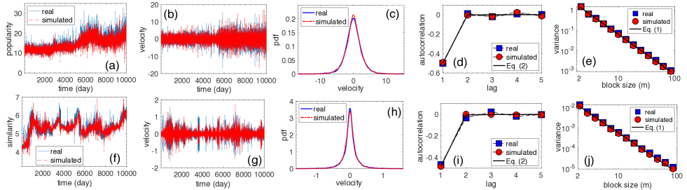
Figure 5: Real vs. simulated trajectories. (a)-(e) juxtapose the radial popularity trajectory of CLT in the US Air transportation network (blue lines and markers) against its simulated counterpart (red lines and markers) constructed using the fBm model described in the text. The simulated trajectory has the same Hurst exponent, time-varying trend, and time-varying variance as the real trajectory. (f)-(j) show the same, but for the similarity trajectory of CLT.

Specifically, we consider a modification of the Riemann-Liouville multifractional Brownian motion model of Ref. Muniandy and Lim (2001), where instead of varying the Hurst exponent over time, we vary the noise-induced variance (see Appendix G). The model aims to capture trajectories that behave only locally, i.e., within intervals of variance stationarity, as an fBm. Further, we note that the velocities may not fluctuate exactly around zero, corresponding to trends in the trajectories; in other words, trajectories may exhibit both trends and a mean-reverting behavior in their increments. This is particularly the case for the radial popularity trajectories, which usually have increasing trends following the trend at which the hyperbolic disc where nodes reside increases (see Figs. 1(a), Fig. 11, and Appendix H). Trends may also exist in the expected degree and similarity trajectories, although they are often less apparent (see Figs. 1(f) and 2(a), and Appendix H). Therefore, we also adjust the model to account for possible trends in the trajectories that can also change with time. The final equation for the considered fBm model takes the form

$$\tilde{B}_{H}(t) =B_{0}+\int_{0}^{t}\mu(s)\mathrm{d}s$$ (3)

$$+\frac{1}{\Gamma{(H+\frac{1}{2})}}\int_{0}^{t}(t-s)^{H-1/2}\sigma(s)\mathrm{d}B(s),~{}~{}t\geq 0,$$

where $B(s)$ is the standard Brownian motion, $B_{0}$ is the initial position, $H\in(0,1)$ is the Hurst exponent, $\Gamma$ is the gamma function, and $\mu(s)$ and $\sigma(s)$ are respectively the trend and noise-induced volatility at time $s$. In Appendix G, we provide the discrete-time analogue of the model and explain how to tune its parameters to create simulated counterparts of real trajectories.

Figure 5 shows that the model can adequately capture the popularity and similarity trajectories of CLT in the US Air transporation network. In general, we find that the model can capture the trajectories of all the considered real networks (see Figs. 16-37 for other examples), apart from some cases (present mainly in PGP and arXiv) where similarity trajectories appear to exhibit jumps. Such cases suggest that modeling extensions that also account for jumps may be desirable, cf. Ref. Xiao et al. (2010). Other modeling extensions may include accounting for non-Gaussian increment structures akin to time-changed fBms Wyłomańska et al. (2016); Kumar et al. (2017). Such extensions are beyond the scope of this paper.

Finally, given the ability of the considered fBm model to simulate trajectories resembling real ones, a natural next question is whether the considered model can also be used for predicting the future evolution of the real trajectories, such as the area in which the trajectories are expected to be located and their expected trend. While a comprehensive assessment of the model’s predictive capabilities is beyond the scope of the present work, we provide a glimpse on the model’s ability for predictions in Appendix I. We show that predictions are possible, even with simple educated guesses on the model’s parameters for the prediction period, based on historical data. This predictability can be explained by the fact that the variance of the considered model grows with time $t$ as $t^{2H}$, where $H$ is the Hurst exponent Mandelbrot and Ness (1968). Therefore, as real trajectories are typically characterized by low values of $H\ll 0.5$ (i.e., displaying strong anti-persistence), their variance grows slowly with time, remaining even approximately constant for cases where $H\approx 0$, favoring their predictability.

Outlook

Description and prediction of network dynamics is a grand-challenge open problem in network science, with important practical applications in diverse domains, including social networks Lazer et al. (2009), recommender systems Uchyigit and Ma (2008), network economics Bramoullé and Kranton (2007), terrorist network modeling Gutfraind (2009), and protein interaction Eronen and Toivonen (2012). Despite decades of research, there is still lack of understanding of fundamental laws driving the dynamics of real networks. Our work unravels and interprets, for the first time, fundamental characteristics of the popularity and similarity trajectories of nodes in hyperbolic embeddings of real networks, and shows that well-developed mathematical machinery from stochastic modeling is applicable for describing their dynamics. Furthermore, by using the model of Eq. (3) and under simple assumptions for its parameters, we provide evidence that predicting the future evolution of the popularity-similarity trajectories of real networks is possible due to their intrinsic characteristics (Appendix I).

These results pave the way towards the ultimate goal of predicting connectivity dynamics in real networks over different time scales. To accomplish this goal, robust methodologies for trajectory prediction should be developed through automated approaches for fine-tuning the parameters of the proposed model or of possible variations of it. Of particular interest are techniques that can predict changes in the expected trends of the trajectories. Other interesting approaches may involve analyzing many trajectories simultaneously, instead of individually as considered here, which could identify possible synchronization phenomena across the trajectories. Predicting connectivity dynamics would then be equivalent to predicting the evolution of hyperbolic distances among node pairs and deciding on their temporal connectivity based on their distance.

Appendix A Real-world network data

Here we provide details on the considered real-world networks. An overview of the data is given in Table 1 of the main text.

US Air. The US Air network corresponds to domestic flights between US airports. The data set is constructed by data available by the US department of transportation USA . Each directed link signifies a flight between a source and destination airport in the US. We consider 10000 topology snapshots corresponding to the period January 1988 to May 2015. Each snapshot is obtained by merging the flight links between the US airports over a one day period. For each of the snapshots we form their undirected counterparts by taking into account only bi-directional links between airports. For each snapshot of the undirected counterparts we isolate the largest connected component. The evolution of the number of nodes, average degree, and average clustering Dorogovtsev (2010) in the network is shown in Fig. 10. In the considered period these quantities evolve in a relatively stable manner. We do not consider data after the aforementioned period as the average clustering in daily snapshots fluctuates rapidly (Fig. 10(c)).

We note that in the considered period, the percentage of new links between consecutive snapshots, i.e., the percentage of links present in snapshot $G_{t}$ but not in $G_{t-1}$ is on average $1.6\%$ with a standard deviation of $1.8$. For the old links between consecutive snapshots, i.e., the links present in snapshot $G_{t-1}$ but not in $G_{t}$, these numbers are respectively $1.6\%$ and $1.9$.

Bitcoin (BTC). The BTC network corresponds to transactions between bitcoin addresses in the bitcoin cryptocurrency network and is constructed by data taken from Ref. btc . Each directed link in the network signifies a bitcoin transaction between a sender and a receiver address. We consider 1292 daily topology snapshots corresponding to the period August 2012 to March 2016. Each snapshot is obtained by merging all the transaction links up to the date of the snapshot. For each of the snapshots we form their undirected counterparts by taking into account only bi-directional transaction links between bitcoin addresses. For each of the undirected counterparts we consider links attached to nodes with degrees $k\geq 4$, and isolate the largest connected component. The evolution of the number of nodes, average degree, and average clustering in the network is shown in Fig. 10. In the considered period these quantities evolve in a relatively stable manner. The percentage of new links between consecutive snapshots is on average $0.14\%$ with a standard deviation of $0.14$. The network is purely growing and therefore there are no link removals.

PGP WoT. Pretty-Good-Privacy (PGP) is an encryption program that provides cryptographic privacy and authentication for data communication ope . PGP web of trust (WoT) is a directed network where nodes are certificates consisting of public PGP keys and owner information. A directed link in the web of trust pointing from certificate A to certificate B represents a digital signature by owner of A endorsing the owner/public key association of B. We use temporal PGP web of trust data collected by Jörgen Cederlöf pgp . Specifically, we consider $1500$ daily PGP topology snapshots spanning the period March 2003 to May 2007. For each of the snapshots we form their undirected counterparts by taking into account only bi-directional trust links between the certificates. For each of the undirected counterparts we consider links attached to nodes with degrees $k\geq 6$, and isolate the largest connected component. The evolution of the number of nodes, average degree, and average clustering in the network is shown in Fig. 10. We do not consider data after the aforementioned period as the number of nodes fluctuates rapidly (Fig. 10(a)). The percentage of new links between consecutive snapshots is on average $0.16\%$ with a standard deviation of $0.52$. For the old links between consecutive snapshots these numbers are respectively $0.06\%$ and $0.49$.

IPv6 Internet. The IPv6 Autonomous Systems (AS) Internet topology snapshots were extracted from data collected by CAIDA Claffy et al. (2009). Pairs of ASs peer to exchange traffic and the links in the AS topology represent peering relationships between ASs. CAIDA’s IPv6 data set as_ provides regular snapshots of AS links. The data set consists of ASs that can route packets with IPv6 destination addresses. We consider 300 topology snapshots, spanning the period October 2011 to July 2017. Each snapshot corresponds to an interval of one week and is obtained by merging the AS links observed in that week. The evolution of the number of nodes, average degree, and average clustering in the network is shown in Fig. 10. In the considered period these quantities evolve in a relatively stable manner. The percentage of new links between consecutive snapshots is on average $6.3\%$ with a standard deviation of $3.8$. For the old links between consecutive snapshots these numbers are respectively $5.8\%$ and $2.3$.

arXiv. The temporal arXiv collaboration network is constructed by data taken from Ref. arx . In arXiv, each paper is assigned to one or more relevant categories. We consider the temporal co-authorship network formed by the authors of papers in the category “Quantitative Finance”. In each topology snapshot the nodes are authors that are connected if they have co-authored a paper. We consider 3977 daily snapshots corresponding to the period August 2011 to July 2022. Each snapshot is obtained by merging all the co-author links up to the date of the snapshot, and isolating the largest connected component. The evolution of the number of nodes, average degree, and average clustering in the network is shown in Fig. 10. The percentage of new links between consecutive snapshots is on average $0.05\%$ with a standard deviation of $0.17$. The network is purely growing and therefore there are no link removals.

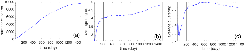
Figure 6: (a) Number of nodes, (b) average degree, and (c) average clustering in the US Air. We consider data up to time 10000 (May 20, 2015) indicated by the vertical line in the plots.

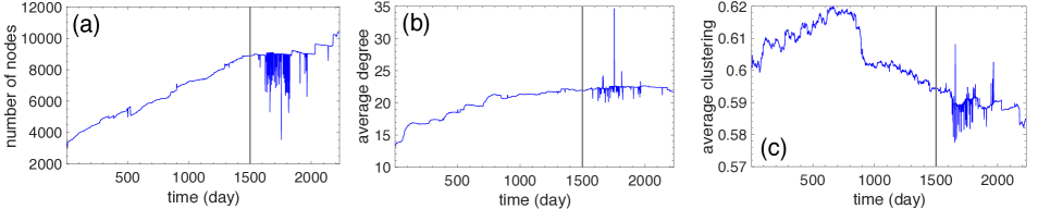
Figure 7: (a) Number of nodes, (b) average degree, and (c) average clustering in the BTC. We consider data after time 200 (August 22, 2012).

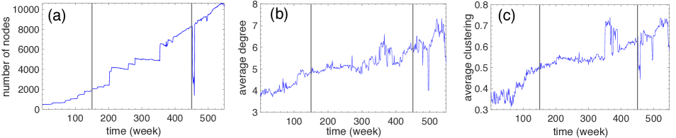
Figure 8: (a) Number of nodes, (b) average degree, and (c) average clustering in the PGP WoT. We consider data up to time 1500 (May 4, 2007).

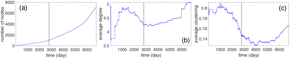
Figure 9: (a) Number of nodes, (b) average degree, and (c) average clustering in the IPv6 Internet. We consider data from time 150 to 450 (October 17, 2011 to July 17, 2017).

Figure 10: (a) Number of nodes, (b) average degree, and (c) average clustering in the arXiv (Quantitative Finance). We consider data after time 2800 (August 1, 2011).

Appendix B Hyperbolic embedding

We map each network snapshot to an underlying hyperbolic space using Mercator García-Pérez et al. (2019). Mercator combines the Laplacian Eigenmaps approach of Ref. Muscoloni et al. (2017) with maximum likelihood estimation, used also in previous methods Boguñá et al. (2010); Papadopoulos et al. (2015a, b), to produce fast and accurate embeddings. In a nutshell, Mercator takes as input the network’s adjacency matrix $A$. The generic element of the matrix is $A_{ij}=A_{ji}=1$ if there is a link between nodes $i$ and $j$, and $A_{ij}=A_{ji}=0$ otherwise. It then infers radial (popularity) and angular (similarity) coordinates, $r_{i}$ and $\theta_{i}$, for all nodes $i\leq N$. To this end, it maximizes the likelihood function

$$\mathcal{L}=\prod_{1\leq j<i\leq N}p(x_{ij})^{A_{ij}}\left[1-p(x_{ij})\right]^{1-A_{ij}},$$ (4)

where the product goes over all node pairs $i,j$ in the network, while $p(x_{ij})$ is the Fermi-Dirac connection probability,

$$p(x_{ij})=\frac{1}{1+e^{\frac{1}{2T}(x_{ij}-R)}}.$$ (5)

Here, $x_{ij}=r_{i}+r_{j}+2\ln{(\Delta\theta_{ij}/2)}$ is approximately the hyperbolic distance between nodes $i$ and $j$ Krioukov et al. (2010); $\Delta\theta_{ij}=\pi-|\pi-|\theta_{i}-\theta_{j}||$ is the angular similarity distance; $R$ is the radius of the hyperbolic disc where nodes reside; and $T\in(0,1)$ is the network temperature, which is also inferred by Mercator and is related to the clustering strength of the network.

The connections and disconnections among nodes act respectively as attractive and repulsive forces. Mercator feels these attractive/repulsive forces, placing connected (disconnected) nodes closer to (farther from) each other in the hyperbolic space. We note that changes in the adjacency matrix $A$ result in the re-evaluation of all node positions.

The radial coordinate $r$ of a node is related to its expected degree $\kappa$, as

$$r\sim R-2\ln{\kappa}.$$ (6)

The disc radius $R$ grows logarithmically with the network size $N$, $R\sim 2\ln{N}$, and depends also on the average degree and clustering in the network Krioukov et al. (2010); García-Pérez et al. (2019). The evolution of $R$ in the considered networks is shown in Fig. 11.

Furthermore, as mentioned in the main text, we also consider the trajectories of expected degrees, i.e., the trajectories of $\kappa$ in (6). We consider these, as they do not directly depend on the evolution of $R$, and are thus more direct proxies to the evolution of individual node popularities. In contrast, $R$ can significantly dominate in (6), rendering the evolution of individual popularities via radial coordinates less apparent.

The code implementing Mercator is made publicly available at mer (2019). We have used the code without any modifications. To minimize fluctuations due to random number generation we use the same random seed value for embedding the snapshots of a given network.

Appendix C Procrustean rotations

The distances between the nodes in the embeddings are invariant with respect to global rotations and reflections of the angular coordinates. Thus, given the embeddings $E_{t-1}$ and $E_{t}$ of two consecutive snapshots $G_{t-1}$ and $G_{t}$, the angles in $E_{t}$ can be globally shifted compared to the angles in $E_{t-1}$. To mitigate such effects, we apply the following procedure.

Let $\mathcal{S}=E_{1},E_{2},\ldots,E_{\tau}$ be the sequence of embeddings of snapshots $G_{1},G_{2},\ldots,G_{\tau}$. We consider the nodes’ angular trajectories in the sequence of optimally rotated embeddings, $\mathcal{S^{\textnormal{r}}}=E_{1}^{\textnormal{r}},E_{2}^{\textnormal{r}},\ldots,E_{\tau}^{\textnormal{r}}$, obtained as follows. First, $E_{1}^{\textnormal{r}}$ is the same as $E_{1}$. Then, each successive embedding $E_{t}^{\textnormal{r}}$, $t=2,\ldots,\tau$, is obtained by globally shifting the nodes’ angles in $E_{t}$ such that the sum of the squared distances (SSD) between the nodes’ angles in $E_{t}$ and the angles of the corresponding nodes in $E_{t-1}^{\textnormal{r}}$ is minimized. To this end, we apply a Procrustean rotation Rohlf and Slice (1990), as follows:

1. Let $\{\theta_{t-1}^{i}\}$ and $\{\theta_{t}^{i}\}$ be the sets of node angles in $E_{t-1}^{\textnormal{r}}$ and $E_{t}$, respectively. We transform the angles to Cartesian coordinates $\{x_{i},y_{i}\}=\{\cos{\theta_{t-1}^{i}},\sin{\theta_{t-1}^{i}}\}$ and $\{w_{i},z_{i}\}=\{\cos{\theta_{t}^{i}},\sin{\theta_{t}^{i}}\}$.

2. A rotation of the points $\{w_{i},z_{i}\}$ by an angle $\phi$ is given by

   $$\{u_{i},v_{i}\}=\{w_{i}\cos\phi-z_{i}\sin\phi,$$

   $$w_{i}\sin\phi+z_{i}\cos\phi\},$$ (7)

   where $u_{i},v_{i}$ are the coordinates of the rotated point $w_{i},z_{i}$. The SSD between $\{u_{i},v_{i}\}$ and $\{x_{i},y_{i}\}$ is

   $$\textnormal{SSD}=\sum_{i\in\mathcal{C}}(u_{i}-x_{i})^{2}+(v_{i}-y_{i})^{2}.$$ (8)

   The sum is taken over the set of nodes $\mathcal{C}$ that exist in both $E_{t-1}^{\textnormal{r}}$ and $E_{t}$. The optimal rotation angle $\phi^{*}$ is computed by taking the derivative of the SSD with respect to $\phi$ and solving for $\phi$ when the derivative is zero,

   $$\phi^{*}=\tan^{-1}\left[\frac{\sum_{i\in\mathcal{C}}(w_{i}y_{i}-z_{i}x_{i})}{\sum_{i\in\mathcal{C}}(w_{i}x_{i}+z_{i}y_{i})}\right].$$ (9)

   The optimally rotated angles are then computed as

   $$\{\theta_{\textnormal{rotated}}^{i}\}=\{\tan^{-1}(v_{i}^{*}/u_{i}^{*})\},$$ (10)

   where

   $$\{u_{i}^{*},v_{i}^{*}\}=\{w_{i}\cos{\phi^{*}}-z_{i}\sin{\phi^{*}},$$

   $$w_{i}\sin{\phi^{*}}+z_{i}\cos{\phi^{*}}\}.$$ (11)

   We note that if $\theta_{\textnormal{rotated}}^{i}<0$, then $\theta_{\textnormal{rotated}}^{i}\coloneqq 2\pi+\theta_{\textnormal{rotated}}^{i}$.

3. We repeat the above procedure after replacing $\{\theta_{t}^{i}\}$ with $\{2\pi-\theta_{t}^{i}\}$, which is the reflection of the former across the $x$-axis, and compute the optimally rotated angles in this case as well, $\{\tilde{\theta}_{\textnormal{rotated}}^{i}\}$.

4. Finally, we compute $D_{\theta}=\sum_{i\in\mathcal{C}}|\theta_{\textnormal{rotated}}^{i}-\theta_{t-1}^{i}|$ and $\widetilde{D}_{\theta}=\sum_{i\in\mathcal{C}}|\tilde{\theta}_{\textnormal{rotated}}^{i}-\theta_{t-1}^{i}|$. The optimally rotated angles are $\{\theta_{\textnormal{rotated}}^{i}\}$ if $D_{\theta}<\widetilde{D}_{\theta}$, and $\{\tilde{\theta}_{\textnormal{rotated}}^{i}\}$ otherwise. $E_{t}^{\textnormal{r}}$ is obtained from $E_{t}$ by replacing the nodes’ angles in the latter with their optimally rotated angles.

Appendix D Hurst exponent estimation

There exists a variety of techniques for estimating the Hurst exponent $H$ of a time series Taqqu et al. (1995). Here we use the method of absolute moments or generalized exponents Preis et al. (2009); Górski et al. (2002), which involves calculating the sample moments of a time series at different lags and then fitting a linear regression model to estimate $H$.

Specifically, for a time series $g(t)$ with $t\in\{1,2,\ldots,\tau\}$ the time lag-dependent generalized Hurst exponent, $H_{q}(l)$, can be determined by the general relationship Preis et al. (2009); Górski et al. (2002)

$$S_{q}(l)=\langle|g(t+l)-g(t)|^{q}\rangle\propto l^{qH_{q}(l)},$$ (12)

where $q>0$, while $l\ll\tau$ is the time lag, $l=1,2,3,\ldots$. The brackets $\langle\ldots\rangle$ denote the expectation value over $t$.

To estimate the Hurst exponent $H$ of a time series we leverage Eq. (12). First, we compute $S_{q}(l)$ for different lags $l=1,2,\ldots,l_{\textnormal{max}}$, and orders $q=1,2,\ldots,q_{\textnormal{max}}$. Then, for each order $q$, we find the best fit line (in a least-squares sense) for $\log{S_{q}(l)}$ against $\log{l}$. From the slope $\lambda$ of this line we estimate the generalized Hurst exponent $H_{q}=\lambda/q$. Finally, we estimate $H$ as the average of $H_{q}$. In our analysis, we use $q_{\textnormal{max}}=3$ and $l_{\textnormal{max}}=10$, except for the arXiv where we use $l_{\textnormal{max}}=20$ (as $l_{\textnormal{max}}=10$ in this case appeared to sometimes overestimate $H$).

We note that for the radial trajectories $r(t)$, $g(t)$ in Eq. (12) is simply $g(t)=r(t)$. The same holds for the degree trajectories $\kappa(t)$. For the similarity trajectories $\theta(t)$, the situation is a bit more involved as the motion takes place on a circle. In that case, Eq. (12) is not applied on $\theta(t)$ per se, but on the unwrapped similarity trajectories $\theta_{\textnormal{u}}(t)$, i.e., $g(t)=\theta_{\textnormal{u}}(t)$, where $\theta_{\textnormal{u}}(t)$ is computed as described in Appendix E.

We also considered other methods for estimating $H$, such as rescaled range (R/S) analysis Taqqu et al. (1995), reaching similar conclusions. We prefer the method of moments described above, as we found it the most accurate in estimating low values of $H$.

Appendix E Velocities and unwrapped similarity trajectories

The increment or velocity process $v(t),t=2,3,\ldots$, for the radial trajectories is simply given by $v(t)=r(t)-r(t-1)$, and for the degree trajectories by $v(t)=\kappa(t)-\kappa(t-1)$. For the similarity trajectories it is given by

$$v(t)=s\Delta\theta(t),$$ (13)

where $\Delta\theta(t)=\pi-|\pi-|\theta(t)-\theta(t-1)||$ is the angular distance between positions $\theta(t)$ and $\theta(t-1)$, and $s$ is $1$ or $-1$ depending on the direction of the motion (counterclockwise or clockwise). For all trajectories we define $v(1)=0$.

The direction $s$ in Eq. (13) can be computed using the cross product. Specifically, let

$$\{u_{x},u_{y}\}= \{\cos{\theta(t-1)},~{}\sin{\theta(t-1)}\},$$ (14)

$$\{v_{x},v_{y}\}= \{\cos{\theta(t)},~{}\sin{\theta(t)}\}.$$ (15)

Then,

$$s=\text{sgn}(u_{x}v_{y}-u_{y}v_{x}),$$ (16)

where $\text{sgn}(x)$ is the sign function.

The unwrapped similarity trajectories $\theta_{\text{u}}(t)$, are given by

$$\theta_{\text{u}}(t)=\theta(1)+\sum_{i=1}^{t}v(t).$$ (17)

Intuitively, $\theta_{\text{u}}(t)$ is an unfolding of $\theta(t)$, such that the similarity motion takes place on the real line. This allows us to directly compute quantities, like the one given by Eq. (12), which assume that the process is evolving on an unbounded domain. In contrast, in the original representation, $\theta(t)$, the motion takes place on the circle $[0,2\pi]$, i.e., on a bounded domain with periodic boundary conditions (a node passing through one side of the domain $[0,2\pi]$, appears on the other side).

Plotting similarity trajectories. Freed by boundaries, the representation $\theta_{\text{u}}(t)$ also allows us to more clearly visualize the similarity motion. We use this representation whenever we plot similarity trajectories (i.e., we plot $\theta_{\text{u}}(t)$ instead of $\theta(t)$). We note that one can revert back to $\theta(t)$ from $\theta_{\text{u}}(t)$ as follows. Let $m(t)=\textnormal{mod}[\theta_{\text{u}}(t),2\pi]$. Then, $\theta(t)=m(t)$ if $m(t)>0$, otherwise $\theta(t)=2\pi+m(t)$.

Randomized trajectories. Let $v(t),t=2,3,\ldots$, be the velocity process of a real trajectory, and $X(1)$ the trajectory’s initial value. To construct the randomized counterpart of the trajectory, $X^{\textnormal{r}}(t)$, we proceed as follows. First, we randomize the signs of the velocities, while preserving their magnitude, i.e., we create the velocity process $v^{\textnormal{r}}(t)=\tilde{s}|v(t)|$, where $\tilde{s}=1$ or $\tilde{s}=-1$ with probability $0.5$. Then, we compute $X^{\textnormal{r}}(t)$ as

$$X^{\textnormal{r}}(t)=X(1)+\sum_{i=1}^{t}v^{\textnormal{r}}(t).$$ (18)

Appendix F Evolution of hyperbolic discs and Hurst exponents for radial trajectories

Figure 11 shows the evolution of the radius $R$ of the hyperbolic disc, where nodes reside, in the considered networks. We see that in all cases the trajectory of $R$ is also strongly anti-persistent. Further, Fig. 12 shows the distributions of Hurst exponents for the radial popularity trajectories in the considered networks, as in Fig. 3 of the main text.

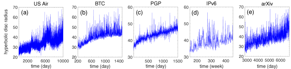
Figure 11: Evolution of the hyperbolic disc radius in the considered networks. The estimated Hurst exponents in (a) to (e) are respectively $0.0008$, $0.003$, $0.007$, $0.003$, and $0.11$.

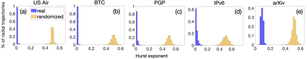
Figure 12: Distributions of Hurst exponents for the radial trajectories in the considered real networks (in blue) and for the randomized counterparts of the trajectories (in yellow). The average Hurst exponents in (a) to (e) for the real trajectories are respectively $0.004$, $0.005$, $0.01$, $0.02$, and $0.09$.

Appendix G Fractional Brownian motion model

As mentioned in the main text, the trajectories can be adequately captured by a fractional Brownian motion model. Specifically, we build on the fractional Brownian motion based on the Riemann-Liouville fractional integral (RL-fBm), defined as

$$B_{H}(t)=\frac{1}{\Gamma{(H+\frac{1}{2})}}\int_{0}^{t}(t-s)^{H-1/2}\mathrm{d}B(s),~{}~{}t\geq 0,$$ (19)

where $B(s)$ is the standard Brownian motion, $H\in(0,1)$ is the Hurst exponent, and $\Gamma$ is the gamma function, cf. Muniandy and Lim (2001). The RL-fBm corresponds to processes with finite starting time, and for sufficiently large times $t$ it is equivalent to the standard fBm Lim (2001).

To generate $N$ points from an RL-fBm, one can use the discrete simulation scheme described in Refs. Muniandy and Lim (2001); Rambaldi and Pinazza (1994). In that scheme, Eq. (19) is approximated by

$$B_{H}(t_{j})=\frac{1}{\Gamma{(H+\frac{1}{2})}}\sum_{i=1}^{j}\int_{(i-1)\Delta t}^{i\Delta t}(t_{j}-\tau)^{H-1/2}\mathrm{d}B(\tau),$$ (20)

where $\Delta t=1/(N-1)$ is the time step; $t_{j}=j\Delta t$, $j=1,2,\ldots,N$, are the discrete time points; and $\mathrm{d}B(\tau)$ is the increment of Brownian motion,

$$\mathrm{d}B(\tau)=\left(\frac{\xi_{i}}{\sqrt{\Delta t}}\right)d\tau,$$ (21)

where $\xi_{i}$ is a discrete sequence of Gaussian white noise with zero mean and unit variance. Upon integration Eq. (20) gives

$$B_{H}(t_{j})=\sum_{i=1}^{j}\xi_{i}w_{j-i+1}\sqrt{\Delta t},$$ (22)

where $w_{i}$ is a weighting function, whose improved form is Muniandy and Lim (2001); Rambaldi and Pinazza (1994)

$$w_{i}=\frac{1}{\Gamma{(H+\frac{1}{2})}}\left[\frac{t_{i}^{2H}-(t_{i}-\Delta t)^{2H}}{2H\Delta t}\right]^{1/2}.$$ (23)

Equations (22) and (23) form the basis of the simulation scheme. Code implementing this scheme is available at giannit (2022).

To simulate trajectories we use a generalization of the above scheme, which accounts for a possibly changing trend and variance, as well as for a non-zero initial position. In this generalization, $B_{H}(t_{j})$ in Eq. (22) is replaced by

$$\tilde{B}_{H}(t_{j})=B_{0}+\sum_{i=1}^{j}\left(\mu_{i}+\sigma_{i}\xi_{i}w_{j-i+1}\sqrt{\Delta t}\right).$$ (24)

In the last relation, $B_{0}$ is the initial position, while $\mu_{i}$ and $\sigma_{i}$ are respectively the trend and noise-induced volatility at time step $t_{i}$. Specifically, in our case $B_{0}$ is the starting position of the popularity or similarity trajectory we want to simulate, $H$ is the trajectory’s estimated Hurst exponent, and $\mu_{i}$ and $\sigma_{i}$ are estimated from the data as described below. The continuous-time analogue of Eq. (24) is Eq. (3) in the main text.

G.1 Estimation of $\mu_{i}$

Given the velocity series $v(t)$, $t=1,2,\ldots$, of a popularity or similarity trajectory (computed as described in Appendix E), we estimate $\mu_{i}$, $i=1,2,\ldots$, using the following exponentially weighted moving average scheme

$$\mu_{1} =v(1),$$

$$\mu_{i} =\alpha v(i)+(1-\alpha)\mu_{i-1},~{}~{}~{}i=2,3,\ldots.$$ (25)

Here, $\alpha\in[0,1]$ denotes the smoothing factor. Lower values of $\alpha$ assign less weight to recent measurements and short-term fluctuations, allowing for capturing longer-term trends. For all of our computations we use $\alpha=0.01$, except for the angular trajectories of the IPv6, where we use $\alpha=0.1$ (here a higher value of $\alpha$ appeared necessary in order to better capture the trajectories).

G.2 Estimation of $\sigma_{i}$

Let $v(t)$, $t=1,2,\ldots,\tau$, be the velocity series of a popularity or similarity trajectory (Appendix E). For each point $t$ we consider a window of length at most $k$ around it, i.e., we consider all $t^{\prime}\in[\text{max}\{1,t-k/2\},\text{min}\{t+k/2,\tau\}]$, and compute the local growth rate

$$S_{k}(t)=\langle|v(t^{\prime})|\rangle_{k}.$$ (26)

The brackets $\langle\ldots\rangle_{k}$ denote the expectation value over $t^{\prime}\in[\text{max}\{1,t-k/2\},\text{min}\{t+k/2,\tau\}]$, while $k/2$ is assumed to be an integer.

Now, consider the increments $v(t)=B_{H}(t+\Delta t)-B_{H}(t)$ of a discretized fBm process $B_{H}(t)$, where $\Delta t$ is the time step. It can be shown, cf. Bianchi (2005), that

$$\langle|v(t)|\rangle=\frac{\sqrt{2}}{\Gamma{(\frac{1}{2})}}\sigma_{H}\sigma\Delta t^{H},$$ (27)

where $\sigma$ is the noise-induced volatility, while $\sigma_{H}$ is the $H$-induced volatility,

$$\sigma_{H}=\sqrt{\frac{\Gamma{(1-2H)}\cos{(H\pi)}}{H\pi}}.$$ (28)

For the case of $\tilde{B}_{H}(t_{j})$ in Eq. (24), we can assume that Eq. (27) holds locally, i.e., within a stationarity window of length $k$ around each point $t_{j}$. Therefore, to have similar local growth rates as in the real trajectory, we estimate $\sigma_{i}$, $i=1,2,\dots$, as

$$\sigma_{i}=\frac{\Gamma{(\frac{1}{2})}}{\sqrt{2}\sigma_{H}}S_{k}(i)\Delta t^{-H},$$ (29)

where $S_{k}(i)$ is given by Eq. (26) and $\Delta t=1/(N-1)$.

The above approach for computing local noise-induced volatilities is similar in spirit to the approach used in Ref. Muniandy and Lim (2001) for computing local Hurst exponents. As in Ref. Muniandy and Lim (2001), for all of our computations we arbitrarily fix $k=8$, bearing in mind that smaller values of $k$ give better accuracy but larger fluctuations, and vice versa.

Appendix H Examples of popularity-similarity trajectories

Figures 16-32 show examples of radial popularity and angular similarity trajectories in the considered real networks, as in Fig. 5 of the main text. The figures also show realizations of simulated counterpart trajectories (in red color) constructed as described in Appendix G. The caption in each figure indicates the network, the id of the corresponding node in the data, and the estimated Hurst exponents of its popularity and similarity trajectories, denoted respectively by $H_{\textnormal{pop}}$ and $H_{\textnormal{sim}}$, and computed as described in Appendix D. Figures 37-37 show examples of expected degree trajectories. In each case the estimated Hurst exponent $H_{\kappa}$ is given in the figure caption.

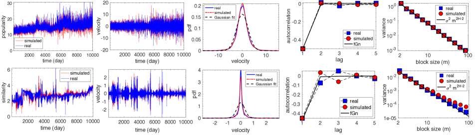
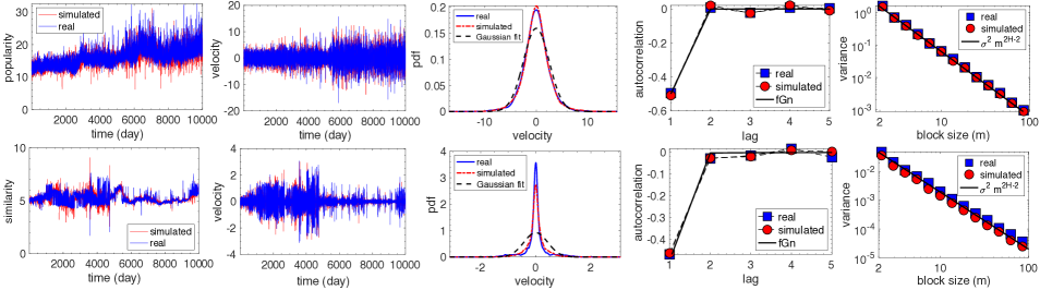
Figure 13: US Air, node LAX (Los Angeles International Airport). $H_{\textnormal{pop}}=0.001$, $H_{\textnormal{sim}}=0.03$.

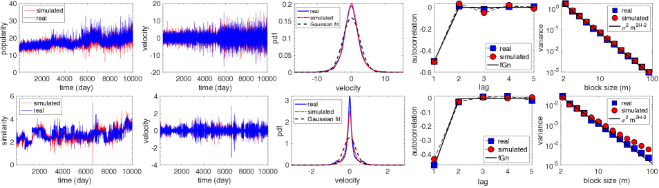
Figure 14: US Air, node BOS (Boston Logan International Airport). $H_{\textnormal{pop}}=0.001$, $H_{\textnormal{sim}}=0.01$.

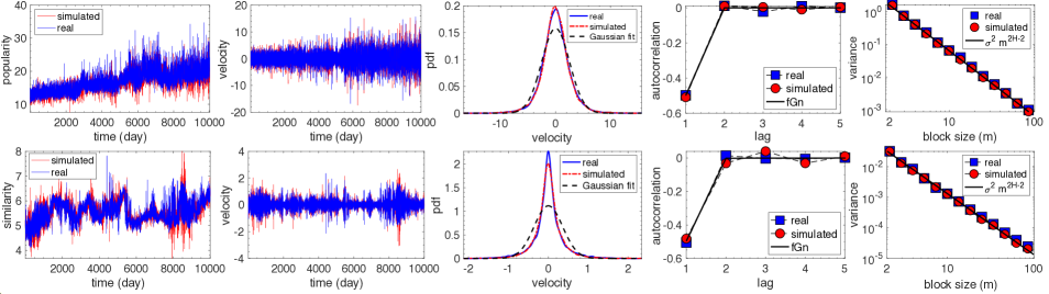
Figure 15: US Air, node SAN (San Diego International Airport). $H_{\textnormal{pop}}=0.001$, $H_{\textnormal{sim}}=0.02$.

Figure 16: US Air, node LGA (LaGuardia Airport). $H_{\textnormal{pop}}=0.001$, $H_{\textnormal{sim}}=0.005$.

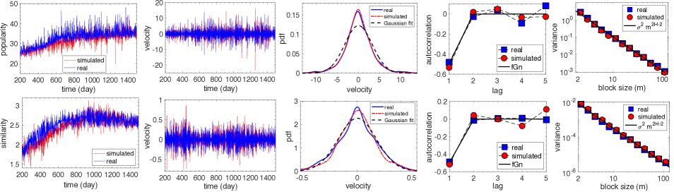
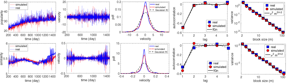
Figure 17: BTC, node 146036. $H_{\textnormal{pop}}=0.002$, $H_{\textnormal{sim}}=0.005$.

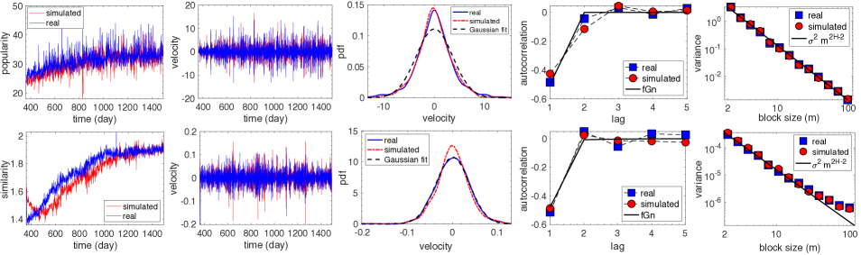
Figure 18: BTC, node 113864. $H_{\textnormal{pop}}=0.004$, $H_{\textnormal{sim}}=0.01$.

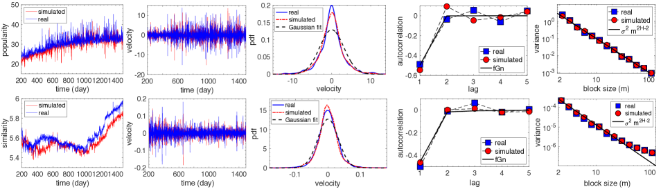
Figure 19: BTC, node 1097470. $H_{\textnormal{pop}}=0.0001$, $H_{\textnormal{sim}}=0.03$.

Figure 20: BTC, node 30238. $H_{\textnormal{pop}}=0.002$, $H_{\textnormal{sim}}=0.06$.

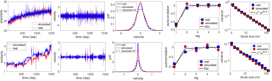
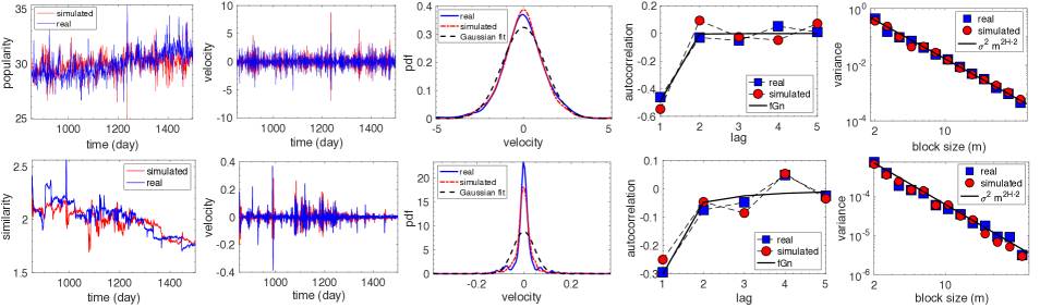
Figure 21: PGP, node 0x0D62001B. $H_{\textnormal{pop}}=0.01$, $H_{\textnormal{sim}}=0.13$.

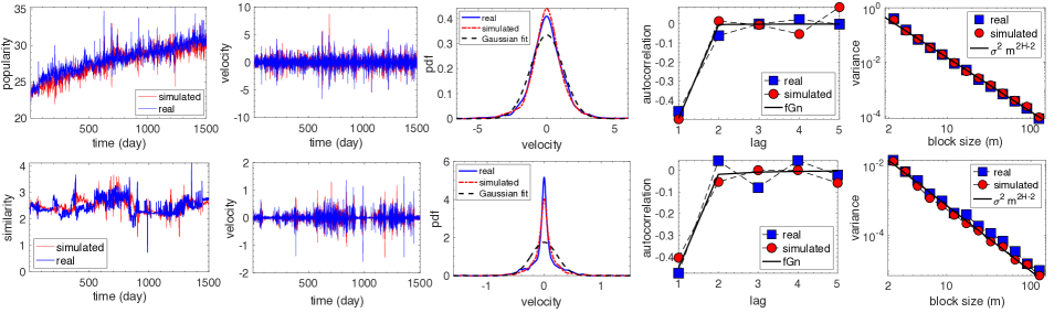
Figure 22: PGP, node 0x0A84BCF5. $H_{\textnormal{pop}}=0.02$, $H_{\textnormal{sim}}=0.24$.

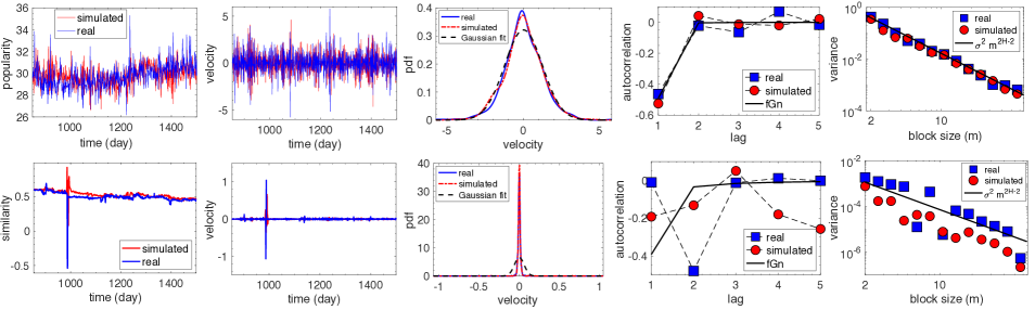
Figure 23: PGP, node 0x0CD8EF97. $H_{\textnormal{pop}}=0.01$, $H_{\textnormal{sim}}=0.07$.

Figure 24: PGP, node 0x0A23A932. $H_{\textnormal{pop}}=0.01$, $H_{\textnormal{sim}}=0.14$.

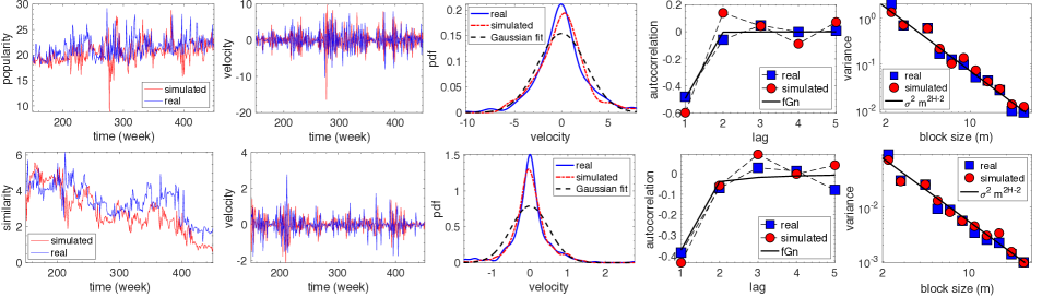
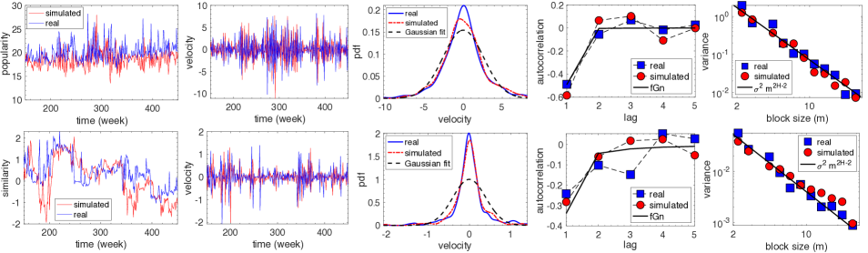
Figure 25: IPv6, node 1239 (Sprint). $H_{\textnormal{pop}}=0.01$, $H_{\textnormal{sim}}=0.17$.

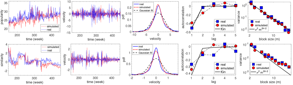
Figure 26: IPv6, node 3320 (Deutsche Telekom). $H_{\textnormal{pop}}=0.01$, $H_{\textnormal{sim}}=0.20$.

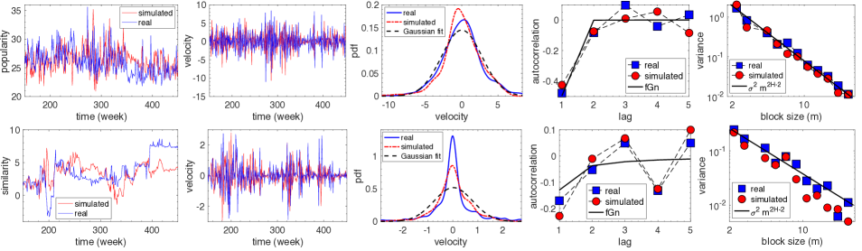
Figure 27: IPv6, node 5539 (SpaceNet). $H_{\textnormal{pop}}=0.007$, $H_{\textnormal{sim}}=0.10$.

Figure 28: IPv6, node 14840 (BR Digital). $H_{\textnormal{pop}}=0.006$, $H_{\textnormal{sim}}=0.40$.

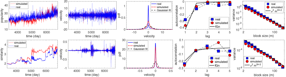
Figure 29: arXiv, node 1058. $H_{\textnormal{pop}}=0.11$, $H_{\textnormal{sim}}=0.28$.

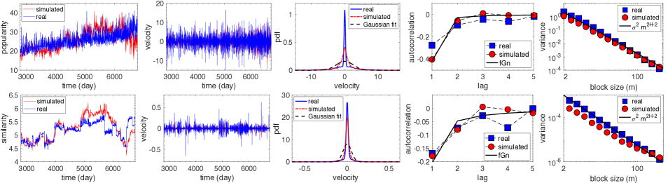
Figure 30: arXiv, node 1218. $H_{\textnormal{pop}}=0.10$, $H_{\textnormal{sim}}=0.34$.

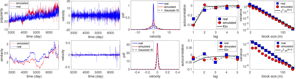
Figure 31: arXiv, node 1827. $H_{\textnormal{pop}}=0.11$, $H_{\textnormal{sim}}=0.34$.

Figure 32: arXiv, node 1674. $H_{\textnormal{pop}}=0.11$, $H_{\textnormal{sim}}=0.46$.

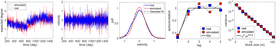
Figure 33: US Air, node SAN. $H_{\kappa}=0.01$.

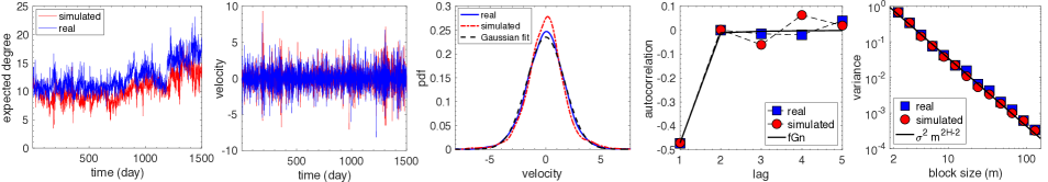
Figure 34: BTC, node 113864. $H_{\kappa}=0.004$.

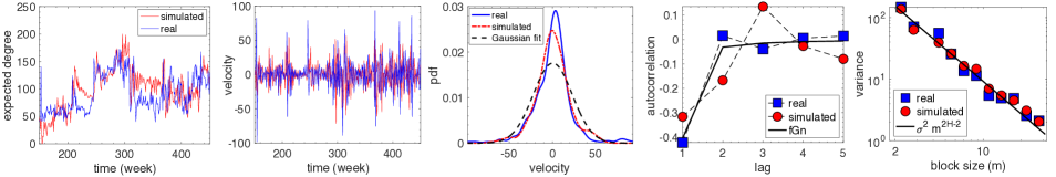
Figure 35: PGP, node 0x0D62001B. $H_{\kappa}=0.04$.

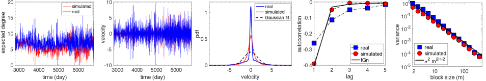
Figure 36: IPv6, node 1239. $H_{\kappa}=0.13$.

Figure 37: arXiv, node 1058. $H_{\kappa}=0.13$.

Appendix I A glimpse on predictability

Appendix H shows that we can construct simulated trajectories resembling the real ones, using the model of Appendix G, i.e., Eq. (24). In principle, the same model can be used for predictions, i.e., for predicting the future evolution of the trajectories, such as the area in which the trajectories are expected to be located and their expected trend. To this end, one will need to make an educated guess for the model’s parameters during the prediction period, i.e., for the values of $H$, $\mu_{i}$, and $\sigma_{i}$, based on historical data.

Figures 42 to 42 illustrate this idea. Here we use the first $80$% of each trajectory as historical data, where we estimate $H$, $\mu_{i}$, and $\sigma_{i}$, as described in Appendix G. Then, we predict the evolution of the subsequent $20$% of each trajectory. For the predictions we simply use the historical estimate of $H$, a constant volatility $\sigma_{i}=\sigma$ equal to the average of the historical $\sigma_{i}$, and a constant trend $\mu_{i}=\mu$ equal to the average of the historical $\mu_{i}$. (In Fig. 42(c), $\mu$ is equal to the average of $\mu_{i}$ from the preceding year, rather than encompassing the entire historical range of $\mu_{i}$.) We find that in several cases this simple approach yields reasonable prediction results, as in Figs. 42-42. Identifying the best automated approaches for fine-tuning the model’s parameters for predictions and performing a comprehensive evaluation of the model’s predictive capabilities are beyond the scope of this paper.

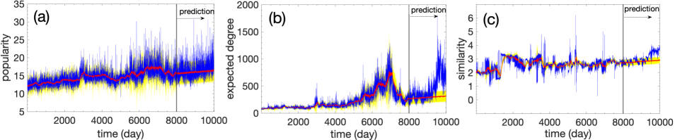
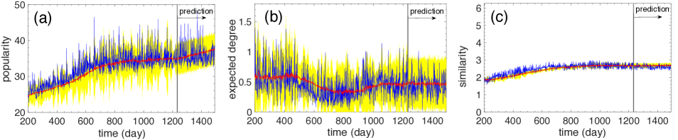
Figure 38: Prediction of the popularity-similarity trajectories of node LAX in the USAir. The real trajectories are shown in blue. The red line is the average across $100$ simulated trajectories constructed using the model of Appendix G. In (a) and (b) the yellow-shaded area stands for two standard deviations away from the average. In (c) it stands for one standard deviation. The model parameters for the prediction period are estimated using the data up to the vertical line (see text). Predictions start immediately after the vertical line.

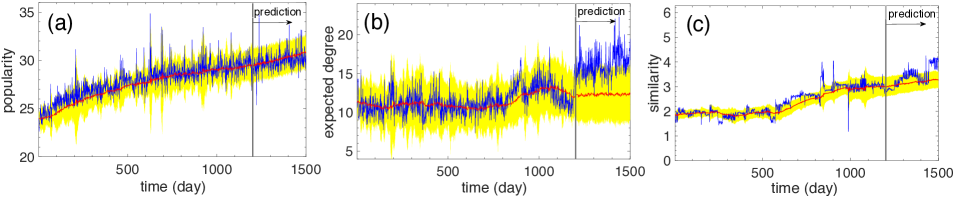
Figure 39: Same as in Fig. 42, but for node 146036 in BTC.

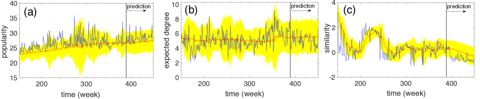
Figure 40: Same as in Fig. 42, but for node 0x0D62001B in PGP WoT.

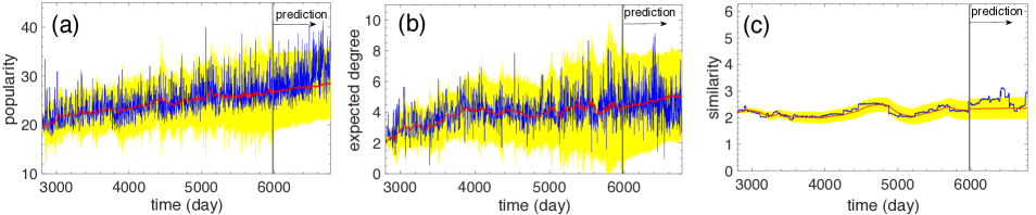
Figure 41: Same as in Fig. 42, but for node 5539 in IPv6.

Figure 42: Same as in Fig. 42, but for node 1674 in arXiv.

Appendix J Popularity-similarity trajectories in geometric vs. non-geometric networks

In this section we provide a detailed description of the temporal network model considered in the main text, along with supplementary figures. The model is based on the $\mathbb{S}^{1}$ model of complex networks Krioukov et al. (2010), which we overview first.

J.1 $\mathbb{S}^{1}$ model

Each node $i$ in the $\mathbb{S}^{1}$ model has hidden variables $\kappa_{i},\theta_{i}$. The hidden variable $\kappa_{i}$ is the node’s expected degree in the resulting network, while $\theta_{i}$ is the angular (similarity) coordinate of the node on a circle of radius $\hat{R}=N/(2\pi)$, where $N$ is the total number of nodes. To construct a network that has size $N$, average node degree $\bar{k}$, power law degree distribution with exponent $\gamma>2$, and temperature $T\in(0,1)$, we perform the following steps:

1. Sample the angular coordinates of nodes $\theta_{i}$, $i=1,2,\ldots,N$, uniformly at random from $[0,2\pi]$, and their hidden variables $\kappa_{i}$, $i=1,2,\ldots,N$, from the probability density function

   $$\rho(\kappa)=(\gamma-1)\kappa_{0}^{\gamma-1}\kappa^{-\gamma},$$ (30)

   where $\kappa_{0}=\bar{k}(\gamma-2)/(\gamma-1)$ is the expected minimum node degree;

2. Connect every pair of nodes $i,j$ with probability

   $$p(\chi_{ij})=\frac{1}{1+\chi_{ij}^{1/T}},$$ (31)

   where $\chi_{ij}=\hat{R}\Delta\theta_{ij}/(\mu\kappa_{i}\kappa_{j})$ is the effective distance between $i$ and $j$, $\Delta\theta_{ij}$ is the angular distance, and $\mu=\sin{T\pi}/(2\bar{k}T\pi)$ ensures that the expected degree in the network is $\bar{k}$.

Smaller values of the temperature $T$ favor connections at smaller effective distances and increase the average clustering in the network, which decreases to zero with $T\in(0,1)$. Other forms of $\rho(\kappa)$ can also be used in the model. The model is isomorphic to random hyperbolic graphs (RHGs) after transforming the expected degrees $\kappa_{i}$ to radial coordinates $r_{i}$ via $r_{i}=R-2\ln{(\kappa_{i}/\kappa_{0})}$, where $R\sim 2\ln{N}$ is the radius of the hyperbolic disc Krioukov et al. (2010).

It can be shown Krioukov et al. (2010) that the configuration model, i.e., the ensemble of graphs with given expected degrees Chung and Lu (2002); Park and Newman (2004), is an infinite temperature limit of the $\mathbb{S}^{1}$ model, where the connection probability in (31) becomes

$$p(\kappa_{i},\kappa_{j})=\frac{1}{1+N\bar{k}/(\kappa_{i}\kappa_{j})}.$$ (32)

In this limit, only the nodes’ expected degrees matter, while the similarity distances among the nodes are completely ignored. Thus, the model is not geometric. If we further let $\kappa_{i}=\bar{k}$ for all nodes $i$, then the connection probability in (32) reduces to

$$p=\frac{1}{1+N/\bar{k}}.$$ (33)

In this case, the nodes’ expected degrees do not matter either and the model degenerates to classical random graphs Solomonoff and Rapoport (1951), where each pair of nodes is connected with the same probability and the resulting degree distribution is Poissonian. Both in the configuration model and in random graphs clustering is asymptotically (as $N\to\infty$) zero.

J.2 Link rewirings and popularity-similarity trajectories

In the main text we consider the following simple model of network snapshots $G_{t},t=1,2,\dots,\tau$, that undergo link rewirings. In the geometric version, snapshot $G_{1}$ is constructed according to the $\mathbb{S}^{1}$ model (RHGs). Then, each subsequent snapshot $G_{t}$ is obtained from $G_{t-1}$ as follows. First, we randomly delete a number of links $l$ from $G_{t-1}$. Then, we add $l$ links among node pairs according to the probability in (31), while ensuring that no multi-edges are created and that the average clustering is preserved. The described link rewiring effectively creates snapshots $G_{t}$ with the same statistical properties, including the same degree distribution. Thus, it mimics behavior in real networks, where statistical quantities, such as average degree, shape of degree distribution, clustering strength, etc., are approximately preserved over time or change slowly (cf. Figs. 10-10(b),(c)).

In the non-geometric version of the model, snapshot $G_{1}$ is constructed either according to the configuration model (CM) or to random graphs (RGs), and the addition of links in subsequent snapshots is done according to (32) and (33), respectively. We use the following parameters: $N=300$, $\bar{k}=8$, $\tau=1000$, $l=30$, $\gamma=2.5$, and $T=0.1$. We note that the percentage of link rewirings in each step ($2.5$%) is of the same order as in some of the considered real networks—the US Air and IPv6 (Appendix A). We also note that for the geometric networks the average clustering is $0.79$, which is strong as in real networks (cf. Figs. 10-10(c)). As mentioned in the main text, once the temporal networks are created, we embed them into hyperbolic spaces and obtain the nodes’ popularity and similarity trajectories following the same procedure as in the real networks.

Figure 43 shows that similarity trajectories in the RHGs model possess similar characteristics as in real networks (the figure corresponds to the trajectory shown in Fig. 4(c) in the main text). These results hold irrespective of the distribution of expected degrees $\rho(\kappa)$. Further, we note that strong anti-persistence in the similarity trajectories can appear at both lower and higher values of the temperature parameter $T$ (corresponding respectively to stronger and weaker clustering).

Figures 44 and 45 show corresponding results for the non-geometric version of the model (Fig. 44 corresponds to the trajectory shown in Fig. 4(e) in the main text). The distributions of Hurst exponents across all similarity trajectories in the networks of Figs. 43-45 are shown in Fig. 4(b) in the main text.

Finally, Figs. 46 to 48 show corresponding results for the expected degree trajectories. In the geometric version of the model, these trajectories also possess similar characteristics as in real networks (Fig. 46). As mentioned in the main text, degree anti-persistence weakens in non-geometric networks (Figs. 47, 48). Figure 4(a) in the main text shows the distributions of Hurst exponents across all expected degree trajectories in the considered synthetic networks.

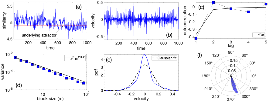
Figure 43: Similarity trajectory in a temporal network constructed according to the $\mathbb{S}^{1}$ model (RHGs). Plots (a) to (f) show the same as in Fig. 2(a) to (f) in the main text. The red line in (a) indicates the node’s hidden similarity coordinate $\theta=4.9$. The estimated Hurst exponent for the trajectory is $0.16$.

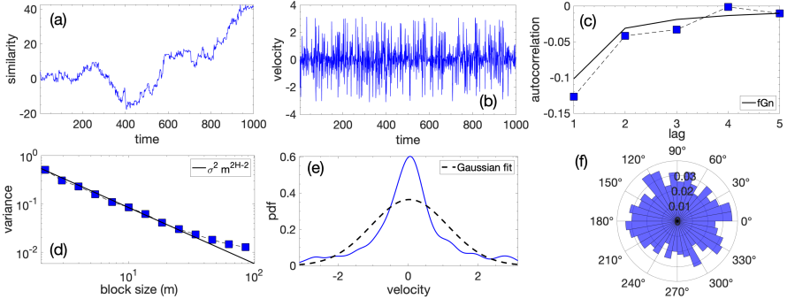
Figure 44: Same as in Fig. 43, but for a trajectory in a temporal network constructed according to CM with the same power-law distribution of expected degrees. The estimated Hurst exponent for the trajectory is $0.42$.

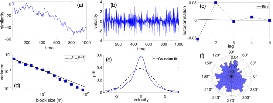
Figure 45: Same as in Fig. 43, but for a trajectory in a temporal network constructed according to RGs with the same expected degree. The estimated Hurst exponent for the trajectory is $0.5$.

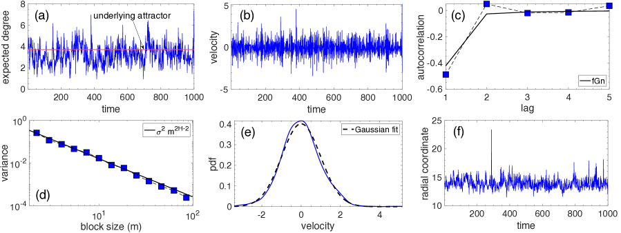
Figure 46: Plots (a)-(e) are the same as in Fig. 43(a)-(e), but for the expected degree trajectory of the corresponding node (RHGs model). The red line in (a) indicates the node’s hidden degree variable $\kappa=3.7$. Plot (f) shows the node’s radial trajectory. The estimated Hurst exponents for the degree and radial trajectories are respectively $0.10$ and $0.04$.

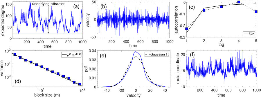
Figure 47: Same as in Fig. 46, but for the expected degree of the node in Fig. 44 (CM). The node’s hidden degree is $\kappa=20.6$ (red line in (a)). The Hurst exponents for the degree and radial trajectories are respectively $0.28$ and $0.04$.

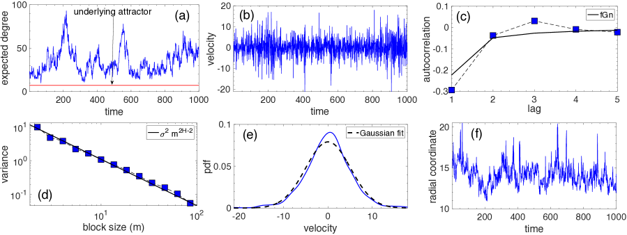
Figure 48: Same as in Fig. 46, but for the expected degree of the node in Fig. 45 (RGs). The node’s hidden degree is $\kappa=7.4$ (red line in (a)). The Hurst exponents for the degree and radial trajectories are respectively $0.32$ and $0.18$.

References

- Krioukov (2014) D. Krioukov, “Brain theory,” Frontiers in Computational Neuroscience 8 (2014), 10.3389/fncom.2014.00114.
- DAR (2007) “DARPA Mathematical Challenges,” (2007), https://web.math.utk.edu/~vasili/refs/darpa07.MathChallenges.html.
- Easley and Kleinberg (2010) D. Easley and J. Kleinberg, Networks, Crowds, and Markets: Reasoning about a Highly Connected World (Cambridge University Press, 2010).
- Alder and Wainwright (1959) B. J. Alder and T. E. Wainwright, “Studies in Molecular Dynamics. I. General Method,” The Journal of Chemical Physics 31, 459–466 (1959).
- Aarseth (2003) S. J. Aarseth, Gravitational N-Body Simulations: Tools and Algorithms, Cambridge Monographs on Mathematical Physics (Cambridge University Press, 2003).
- Schlick (2010) T. Schlick, Molecular Modeling and Simulation: An Interdisciplinary Guide, Interdisciplinary Applied Mathematics (Springer, New York, 2010).
- Friedrich et al. (2011) R. Friedrich, J. Peinke, M. Sahimi, and M. R. R. Tabar, “Approaching complexity by stochastic methods: From biological systems to turbulence,” Physics Reports 506, 87–162 (2011).
- Mandelbrot and Ness (1968) B. B. Mandelbrot and J. W. Van Ness, “Fractional Brownian Motions, Fractional Noises and Applications,” SIAM Review 10, 422–437 (1968).
- Krioukov et al. (2010) D. Krioukov, F. Papadopoulos, M. Kitsak, A. Vahdat, and M. Boguñá, “Hyperbolic geometry of complex networks,” Phys. Rev. E 82, 036106 (2010).
- Boguñá et al. (2010) M. Boguñá, F. Papadopoulos, and D. Krioukov, “Sustaining the Internet with hyperbolic mapping,” Nature Communications 1, 62 EP – (2010).
- Papadopoulos et al. (2012) F. Papadopoulos, M. Kitsak, M. Á. Serrano, M. Boguñá, and D. Krioukov, “Popularity versus similarity in growing networks,” Nature 489, 537 EP – (2012).
- García-Pérez et al. (2019) G. García-Pérez, A. Allard, M Á. Serrano, and M. Boguñá, “Mercator: uncovering faithful hyperbolic embeddings of complex networks,” New Journal of Physics 21, 123033 (2019).
- Boguñá et al. (2021) M. Boguñá, I. Bonamassa, M. De Domenico, S. Havlin, D. Krioukov, and M. Serrano, “Network geometry,” Nature Reviews Physics 3, 114–135 (2021).
- Mandelbrot et al. (1997) B. B. Mandelbrot, A. J. Fisher, and L. E. Calvet, “A Multifractal Model of Asset Returns,” Cowles Foundation Discussion Paper No. 1164 (1997).
- Muniandy and Lim (2001) S. V. Muniandy and S. C. Lim, “Modeling of locally self-similar processes using multifractional Brownian motion of Riemann-Liouville type,” Phys. Rev. E 63, 046104 (2001).
- Leland et al. (1993) W. E. Leland, M. S. Taqqu, W. Willinger, and D. V. Wilson, “On the self-similar nature of ethernet traffic,” in Proceedings of ACM SIGCOMM (ACM, New York, USA, 1993) p. 183–193.
- Liu et al. (1999) J. Liu, Y. Shu, L. Zhang, F. Xue, and O.W.W. Yang, “Traffic modeling based on FARIMA models,” in Proceedings of the IEEE Canadian Conference on Electrical and Computer Engineering, Vol. 1 (1999) pp. 162–167.
- Friedrich and Peinke (1997) R. Friedrich and J. Peinke, “Description of a Turbulent Cascade by a Fokker-Planck Equation,” Phys. Rev. Lett. 78, 863–866 (1997).
- Hadjihosseini et al. (2014) A. Hadjihosseini, J. Peinke, and N. P. Hoffmann, “Stochastic analysis of ocean wave states with and without rogue waves,” New Journal of Physics 16, 053037 (2014).
- Dorogovtsev (2010) S. N. Dorogovtsev, Lectures on Complex Networks (Oxford University Press, Oxford, 2010).
- Saxton (2007) M. J. Saxton, “A biological interpretation of transient anomalous subdiffusion. I. Qualitative model.” Biophys J. 92, 1178–1191 (2007).
- (22) “US Department of Transportation - On-Time: Reporting Carrier On-Time Performance (1987-present),” https://www.transtats.bts.gov/DL_SelectFields.aspx?gnoyr_VQ=FGJ&QO_fu146_anzr=b0-gvzr, Accessed: July, 2023.
- Kosyfaki and Mamoulis (2022) C. Kosyfaki and N. Mamoulis, “Provenance in Temporal Interaction Networks,” in Proceedings of the IEEE International Conference on Data Engineering (ICDE) (2022) pp. 2277–2290.
- (24) “Kaggle - Bitcoin Dataset for analysis,” https://www.kaggle.com/datasets/chrysanthikosyfaki/bitcoin-dataset-for-analysis, Accessed: July, 2023.
- (25) “OpenPGP Web of Trust Dataset,” https://www.lysator.liu.se/~jc/wotsap/wots2/, Accessed: July, 2023.
- (26) “Ark IPv6 Topology Dataset,” https://www.caida.org/catalog/datasets/ipv6_allpref_topology_dataset/, Accessed: July, 2023.
- (27) “Kaggle - arXiv Dataset,” https://www.kaggle.com/datasets/Cornell-University/arxiv, Accessed: July, 2023.
- Rohlf and Slice (1990) F. J. Rohlf and D. Slice, “Extensions of the Procrustes Method for the Optimal Superimposition of Landmarks,” Systematic Biology 39, 40–59 (1990).
- Hurst (1951) H. E. Hurst, “Long-term storage capacity of reservoirs,” Transactions of the American Society of Civil Engineers 116, 770–799 (1951).
- Mandelbrot (1985) B. B. Mandelbrot, “Self-affine fractals and fractal dimension,” Physica Scripta 32, 257 (1985).
- Preis et al. (2009) T. Preis, P. Virnau, W. Paul, and J. J. Schneider, “Accelerated fluctuation analysis by graphic cards and complex pattern formation in financial markets*,” New Journal of Physics 11, 093024 (2009).
- Górski et al. (2002) A. Z. Górski, S. Drożdż, and J. Speth, “Financial multifractality and its subtleties: an example of DAX,” Physica A: Statistical Mechanics and its Applications 316, 496–510 (2002).
- Gatheral et al. (2018) J. Gatheral, T. Jaisson, and M. Rosenbaum, “Volatility is rough,” Quantitative Finance 18, 933–949 (2018).
- Neuman and Rosenbaum (2018) E. Neuman and M. Rosenbaum, “Fractional Brownian motion with zero Hurst parameter: a rough volatility viewpoint,” Electronic Communications in Probability 23, 1 – 12 (2018).
- Chung and Lu (2002) F. Chung and L. Lu, “The average distances in random graphs with given expected degrees,” Proceedings of the National Academy of Sciences 99, 15879–15882 (2002).
- Solomonoff and Rapoport (1951) R. Solomonoff and A. Rapoport, “Connectivity of random nets,” The bulletin of mathematical biophysics 13, 107–117 (1951).
- Xiao et al. (2010) W.-L. Xiao, W.-G. Zhang, X.-L. Zhang, and Y.-L. Wang, “Pricing currency options in a fractional Brownian motion with jumps,” Economic Modelling 27, 935–942 (2010).
- Wyłomańska et al. (2016) A. Wyłomańska, A. Kumar, R. Połoczański, and P. Vellaisamy, “Inverse Gaussian and its inverse process as the subordinators of fractional Brownian motion,” Phys. Rev. E 94, 042128 (2016).
- Kumar et al. (2017) A. Kumar, A. Wyłomańska, R. Połoczański, and S. Sundar, “Fractional Brownian motion time-changed by gamma and inverse gamma process,” Physica A: Statistical Mechanics and its Applications 468, 648–667 (2017).
- Lazer et al. (2009) D. Lazer et al., “Computational Social Science,” Science 323, 721–723 (2009).
- Uchyigit and Ma (2008) G. Uchyigit and M. Y. Ma, eds., Personalization Techniques and Recommender Systems, Series in Machine Perception and Artificial Intelligence, Vol. 70 (WorldScientific, 2008).
- Bramoullé and Kranton (2007) Y. Bramoullé and R. Kranton, “Public goods in networks,” Journal of Economic Theory 135, 478–494 (2007).
- Gutfraind (2009) A. Gutfraind, “Understanding terrorist organizations with a dynamic model,” in Mathematical Methods in Counterterrorism (Springer Vienna, Vienna, 2009) pp. 107–125.
- Eronen and Toivonen (2012) L. Eronen and H. Toivonen, “Biomine: predicting links between biological entities using network models of heterogeneous databases,” BMC Bioinformatics 13, 119 (2012).
- (45) “OpenPGP,” https://www.openpgp.org/, Accessed: July, 2023.
- Claffy et al. (2009) K. Claffy, Young Hyun, K. Keys, M. Fomenkov, and D. Krioukov, “Internet mapping: From art to science,” in Conference For Homeland Security, 2009. CATCH ’09. Cybersecurity Applications Technology (2009) pp. 205–211.
- Muscoloni et al. (2017) A. Muscoloni, J. M. Thomas, S. Ciucci, G. Bianconi, and C. V. Cannistraci, “Machine learning meets complex networks via coalescent embedding in the hyperbolic space,” Nature Communications 8, 1615 (2017).
- Papadopoulos et al. (2015a) F. Papadopoulos, C. Psomas, and D. Krioukov, “Network mapping by replaying hyperbolic growth,” IEEE/ACM Transactions on Networking 23, 198–211 (2015a).
- Papadopoulos et al. (2015b) F. Papadopoulos, R. Aldecoa, and D. Krioukov, “Network geometry inference using common neighbors,” Phys. Rev. E 92, 022807 (2015b).
- mer (2019) “Mercator embedding code,” https://github.com/networkgeometry/mercator (2019), Accessed: July, 2023.
- Taqqu et al. (1995) M. S. Taqqu, V. Teverovsky, and W. Willinger, “Estimators for long-range dependence: an empirical study,” Fractals 3, 785–798 (1995).
- Lim (2001) S. C. Lim, “Fractional Brownian motion and multifractional Brownian motion of Riemann-Liouville type,” Journal of Physics A: Mathematical and General 34, 1301 (2001).
- Rambaldi and Pinazza (1994) S. Rambaldi and O. Pinazza, “An accurate fractional Brownian motion generator,” Physica A: Statistical Mechanics and its Applications 208, 21–30 (1994).
- giannit (2022) giannit, “Fractional and Multifractional Brownian motion generator,” https://github.com/Rabelaiss/mBm (2022), Accessed: July, 2023.
- Bianchi (2005) S. Bianchi, “Pathwise identification of the memory function of multifractional Brownian motion with application to finance,” International journal of theoretical and applied finance 8, 255–281 (2005).
- Park and Newman (2004) J. Park and M. E. J. Newman, “Statistical mechanics of networks,” Phys. Rev. E 70, 066117 (2004).