Anomaly zones for uniformly sampled gene trees under the gene duplication and loss model

Abstract

Recently, there has been interest in extending long-known results about the multispecies coalescent tree to other models of gene trees. Results about the gene duplication and loss (GDL) tree have mathematical proofs, including species tree identifiability, estimability, and sample complexity of popular algorithms like ASTRAL. Here, this work is continued by characterizing the anomaly zones of uniformly sampled gene trees. The anomaly zone for species trees is the set of parameters where some discordant gene tree occurs with the maximal probability. The detection of anomalous gene trees is an important problem in phylogenomics, as their presence renders effective estimation methods to being positively misleading. Under the multispecies coalescent, anomaly zones are known to exist for rooted species trees with as few as four species.

The gene duplication and loss process is a generalization of the generalized linear-birth death process to the rooted species tree, where each edge is treated as a single timeline with exponential-rate duplication and loss. The methods and results come from a detailed probabilistic analysis of trajectories observed from this stochastic process. It is shown that anomaly zones do not exist for rooted GDL balanced trees on four species, but do exist for rooted caterpillar trees, as with the multispecies coalescent.

1 Introduction

The reconstruction of phylogenetic trees often begins with the analysis of molecular sequences of existing species. Probabilistic and computational methods are used to establish rigorous convergence results as the amount of data goes to infinity. The phylogenomic framework is a two-step approach. First, molecular sequences are used to reconstruct gene phylogenies that depict the evolution of a locus within the genome, and the existing computational technology allows practitioners to collectively estimate many gene trees. A simplifying assumption in the phylogenomic approach is that locus sequences are disjoint so that their evolutionary trajectories are roughly independent. Then, the species tree originating the data is constructed from the many independent gene trees.

Even with these simplifying assumptions, species tree estimation is confounded by gene tree heterogeneity. Common sources of heterogeneity include incomplete lineage sorting (ILS) Rannala and Yang (2003), horizontal gene transfer (HGT) Roch and Snir (2013), and gene duplication and loss (GDL) Arvestad et al. (2009). Many theoretical results, positive and negative, have been established when the only source of heterogeneity is ILS, see Degnan and Rosenberg (2006), Allman et al. (2011), and Mirarab et al. (2014). Incomplete lineage sorting is modeled by the multispecies coalescent (MSC) model.

If the gene trees are assumed independent, then the majority rule consensus estimator of the species tree topology coincides with the maximum likelihood estimator of the gene tree topology. Even under these ideal assumptions, there exist species trees for which the majority rule consensus is positively misleading. Such rooted trees exist when the number of species is as few as four. Similarly, majority rule consensus can be positively misleading for some unrooted trees with as few as five species. Species trees are in the anomaly zone if the gene tree with maximum probability is discordant from the species tree (Degnan and Rosenberg (2006)). However, by using supertree methods such as ASTRAL (Mirarab et al. (2014)) on unrooted quartets, any unrooted species tree can be consistently estimated in polynomial time. Finite sample guarantees have also been developed, see Shekhar et al. (2018).

Much less is known about species tree estimation in the presence of GDL. Recently, using probabilistic and cominbatorial arguments, it was shown that majority rule consensus is a consistent estimator of unrooted quartets under GDL (Legried et al. (2021)), so ASTRAL is also consistent when the input data are GDL trees rather than MSC trees. The result was generalized further when gene trees come from the DLCoal model, where GDL and ILS occur simultaneously, see Markin and Eulenstein (2021) and Hill et al. (2022). Finite sample guarantees for ASTRAL have been proven, showing a sufficient amount of data needed to obtain high probability results Hill et al. (2022).

In this paper, the distribution of gene trees is described further for gene trees generated under GDL. With this further information, we describe when anomaly zones can exist for gene trees generated under GDL for rooted species trees on either three or four species. As with anomalous gene trees in the multispecies coalescent model, the lengths of interior edges of the species tree are important. Under GDL as well, species trees with longer interior edges have lower probabilities of discordant gene trees. However, the parameters governing birth and death are also relevant Hill et al. (2022). When the per-capita birth rate is high, the number of edges is high and the signal emitted by the species tree diminishes. Conversely, when the birth rate is 0, gene tree discordance is impossible, unlike with the MSC. Similar effects occur when the death rate is high enough to prevent excessive branching in the GDL process. This paper provides results that aid in intuiting the connection between the birth and death rates and gene tree discordance, but the focus is on the number of copies in the ancestral population rather than the birth and death rates themselves. The main results apply to any choice of birth and death rates and species trees with three or four leaves.

The format of this paper is as follows. In Section 2, we make precise the definition of anomalous gene trees in the GDL context. In Section 3, the population process is recalled, and a short result relating the arithmetic mean and quadratic mean of independent progenies is proved. In Section 4, the relationship between the population process and the species tree is investigated. In Section 5, it is shown that the rooted balanced quartet has no anomaly zones, in contrast to the MSC model. In Section 6, it is shown that the rooted caterpillar quartet may or may not have anomaly zones, but that only balanced gene trees could possibly be anomalous.

2 Problem and model

In this section, we describe the model and state the results.

Let $S$ be the collection of species and $\sigma=(\mathcal{T},\mathbf{f})$ be the species tree with topology $\mathcal{T}=(V,E)$ and branch lengths $\mathbf{f}=\{f_{e}\}_{e\in E}.$ The species tree topology $\mathcal{T}$ contains only the vertices $V$ and the edges $E=\{(u,v)\}_{u,v\in V}.$ The problem is to estimate $\mathcal{T}$ from a collection $\mathcal{G}=\{t_{\iota}\}_{\iota=1}^{K}$ of $K$ multi-labelled gene tree topologies. A gene tree is a depiction of the parental lineages of a gene or multiple gene copies from individuals across several species. The gene tree is multi-labelled in that each leaf is assigned exactly one label from $S$, multiple leaves may be labelled with the same species. By contrast, a gene tree is single-labelled if no species is used more than once in the labelling of leaves. The process of gene duplication may create multiple copies of a gene within the same individual in a species. We refer to these duplicated genomic segments as gene copies and we refer to collections of gene copies from different unrelated genes as gene families. Gene families depict the joint ancestral history of these related gene copies. In contrast, a species tree is a depiction of the evolutionary relationships of a group of species.

Multiple leaves of a gene tree may be labelled by the same species; this corresponds to observing multiple paralogous copies (i.e., which have arisen from gene duplication) of a gene within the genome. In practice, gene trees are estimated from the molecular sequences of the corresponding genomic segments using a variety of phylogenetic reconstruction methods, see Semple and Steel (2003); Felsenstein (2003); Gascuel (2005); Yang (2014); Steel (2016); Warnow (2017). Here, we assume that gene trees are provided without estimation error for a large number of gene families. Our main modeling assumption is that these gene trees have been drawn independently from a distribution for which the species tree $\sigma$ is taken as a fixed parameter. We define the model more precisely next.

Model.

The gene trees are assumed to be independent and identically distributed. There are $\kappa$ gene trees given. The process for generating a gene tree under GDL proceeds in two steps. The process is repeated independently for each $\iota\in\{1,\dots,\kappa\}$.

Starting with a single ancestral copy of a gene at the root of $\mathcal{T}$, a tree is generated by a top-down birth-death process within the species tree,  Arvestad et al. (2009). On each edge in $\mathcal{T}$, each gene copy independently evolves. It duplicates at exponential rate $\lambda\geq 0$ and is lost at exponential rate $\mu\geq 0$. Each gene copy that survives to a speciation vertex in $\mathcal{T}$ undergoes a bifurcation into two child copies, one for each descendant edge of $\mathcal{T}$. The process continues inductively up to the present. The gene tree is then pruned of lost copies. (These lineages cannot be observed.) Species labels are assigned to each leaf from $S$. Each bifurcation in the gene tree arises through duplication or speciation. An intuitive way to view this process is that $\sigma$ is depicted using a fat tree. This tree constrains the linear birth-death process so that it contains a skinny tree. A sampled realization of the GDL process on a tree with three species is given in Figure 1.

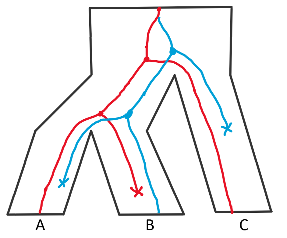
Figure 1: The fat tree is the species tree on the species $A$,$B$,$C$. The skinny tree (colored red and blue) indicates a possible gene tree where no species goes extinct. Note the topology of the pruned tree (nodes labelled “X” died so they are removed from the tree) puts $A$ and $C$ more closely related than $A$ and $B$, showing how discordance can arise under gene duplication and loss.

It is assumed that there is one and only one copy from each species in the gene tree topology $t=t_{\iota}$. Such gene trees generated by GDL have been called “pseudoorthologs”, e.g. Smith and Hahn (2022). In the next few lemmas, we analyze the likelihood function of $t$ under these assumptions. Throughout, the species tree $\sigma=(\mathcal{T},\mathbf{f})$ is assumed to have no more than four leaves. The edge lengths $\mathbf{f}$ are set so that the tree is ultrametric, meaning all leaves have the same distance to the root.

Gene trees under GDL are multi-labelled, in contrast to singly-labelled MSC gene trees, but the singly-labelled GDL gene trees described in the previous paragraph are still highly useful in real-world problems. In the estimation methods ASTRAL-one and ASTRAL-multi for species tree reconstruction (Du et al. (2019), Rabiee et al. (2019), Legried et al. (2021)), multi-labelled gene trees are pre-processed into a collection of singly-labelled trees. We will need only trees generated for ASTRAL-one in this paper. Conditioned on no species going extinct in the multispecies linear birth-death process (this conditioning is acknowledged by $\mathbf{P}^{\prime}$), ASTRAL-one selects one gene copy from each species in the gene family uniformly at random and removes the other lineages from the gene tree. The result is a singly-labelled tree $(u(t),\mathbf{f}(t))$, which we denote $U(t)$. Realizations $U(t)$ are called uniformly sampled gene trees. These singly-labelled gene trees may then be evaluated to find support for different hypotheses of the species tree. In this paper, we describe the distribution of uniformly sampled gene trees, as they have shown to be informative to estimating the species tree.

3 Structured numbers of copies under the GDL process

The GDL process is a generalization of the linear birth-death process, and some of the basic results are recalled here. In the species tree with stem edge of length $s$, let $N_{s}$ be the number of copies at time $s$. The probability mass function of $N_{s}$ is denoted $p_{i}(s)=\mathbf{P}(N_{s}=i).$ Then for any $i\geq 0$:

$$\mathbf{P}(N_{s}=i)=\begin{dcases}\frac{\mu}{\lambda}q(s)&\textnormal{if}\ i=0\\ e^{-(\lambda-\mu)s}\left(1-p_{0}(s)\right)^{2}q(s)^{i-1}&\textnormal{if}\ i>0,\end{dcases}$$

where

$$q(s)=\begin{dcases}\frac{\lambda-\lambda e^{-(\lambda-\mu)s}}{\lambda-\mu e^{-(\lambda-\mu)s}}&\textnormal{if}\ \lambda\neq\mu\\ \frac{\lambda s}{1+\lambda s}&\textnormal{if}\ \lambda=\mu.\end{dcases}$$

The derivation of this modified geometric random variable is provided in Chapter 9 of Steel (2016).

We will utilize all components of the GDL model to perform species tree estimation. As stated in the Introduction, the primary focus will be the observed numbers of copies at speciation nodes in the species tree. We review known results and provide new technical results in the Appendix. The accumulation of these results is presented in the following Theorem.

The basic building block is the chain species tree $\sigma$ where $\mathcal{T}$ has a root node $R$, followed by a single interior node $I$, and one child $J$. Any chain can be generalized to a species tree with branching (i.e. speciation) by appending a subtree to interior nodes like $I$. Let $N_{I}$ be the number of surviving copies to $I$. If $N_{I}$ is known, then for each $j\in\{1,...,N_{I}\}$: one can let $N_{I,j}$ be the number of surviving copies to $J$ that descend specifically from $j$. Of interest is the relationship between the arithmetic mean and geometric mean of the $N_{I,j}$ when the weight of the edge from $I$ to $J$ is $f>0$. For that, we use the moment generating function $M_{f}(\tau)=\mathbf{E}^{\prime}[e^{\tau N_{I,1}}|N_{I}]$ of the progeny obtained by a single individual on the branch between $I$ and $J$. We can use the moment generating function to make precise the relationship between the arithmetic mean and the quadratic mean of independent and identically distributed copies of the modified geometric.

Theorem 1.

Conditioned on the value of $N_{I}\geq 1$, let $N_{I,j}$ be the number of surviving progeny to $J$ for each $j\in\{1,2,...,N_{I}\}$. Then

$$\mathbf{E}^{\prime}\left[\frac{\sum_{j=1}^{N_{I}}N_{I,j}^{2}}{\left(\sum_{j=1}^{N_{I}}N_{I,j}\right)^{2}}\bigg{|}N_{I}\right]=N_{I}\int_{\tau=0}^{\infty}\tau M_{f}^{\prime\prime}(-\tau)M_{f}(-\tau)^{N_{I}-1}\ d\tau.$$

The specific form of $M_{f}(\tau)$ is outlined in the Appendix. Unfortunately, this integral is difficult to compute analytically. However, numerical methods could be useful to characterizing the expectation of this ratio. This result could conceivably be used to give exact expressions for the probability of each tree topology, and an implicit formula is given in Proposition 15. Explicit tools are developed for rooted trees with three species in the Appendix, though the results do not find application beyond those of Legried et al. (2021). In the rest of this paper, we focus on deriving simpler one-sided results to obtain relevant results for rooted trees with four species.

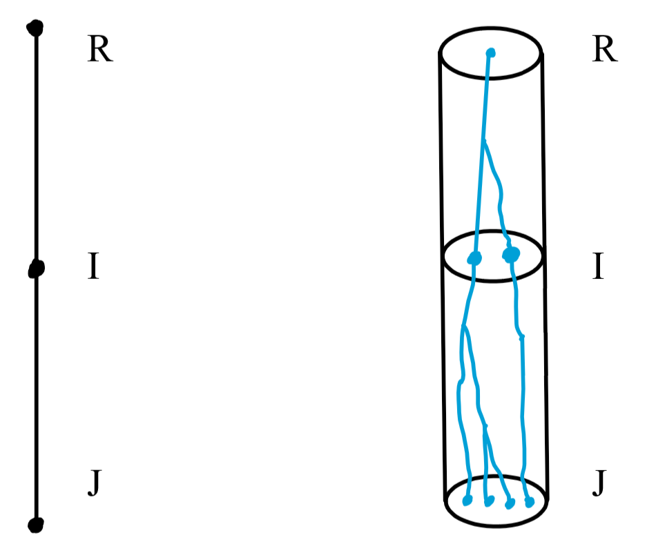
Figure 2: Left: The species tree with root $R$ and subsequent vertices $I$ and $J$. Right: A realization of the GDL process. In the notation of Section 3, this example has $N_{I}=2$ and $N_{I,1}=3$ and $N_{I,2}=1$.

4 Balanced tree on four species

Throughout this section, the species tree $\sigma=(\mathcal{T},\mathbf{f})$ is assumed to have four leaf species $A,B,C,$ and $D$ and the topology has $A,B$ are siblings and $C,D$ are siblings. So, the Newick tree format is $((A,B),(C,D))$. The edge lengths are $s$ for stem edge, $f$ for the parent edge to $A$ and $B$, $g$ for the parent edge to $C$ and $D$, and $f_{n}^{\prime},n\in\{A,B,C,D\}$ for the lengths of pendant edges incident to the leaves. However, we focus on the root vertex, which we label $I$. As suggested in Section 2, let $\mathbf{P}^{\prime}$ be the probability measure subject to the conditioning event where $N_{A},N_{B},N_{C},$ and $N_{D}$ are positive. Let $i_{m},m\in\{a,b,c,d\}$ be the ancestor of sampled copy $m$ at $I$. Conditioning further on $N_{I}$, the probability of each gene tree topology is written using $N_{I}$, using the probabilities $\mathbf{P}^{\prime}_{N_{I}}(i_{a}=i_{b}),$ and $\mathbf{P}^{\prime}_{N_{I}}(i_{c}=i_{d})$.

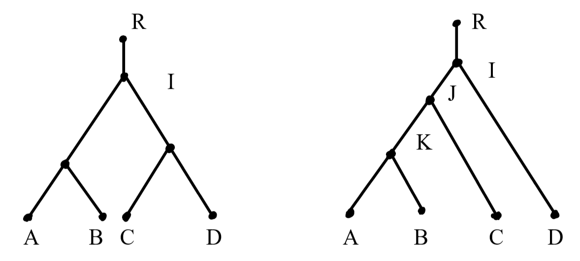
Figure 3: Left: The balanced species tree with species $A,B,C,D$. In Section 5, the length of the edge between $I$ and the parent of $A$ and $B$ is given by $f$, and the length of the edge between $I$ and the parent of $C$ and $D$ is given by $g$. Right: The caterpillar species with species $A,B,C,D$. In Section 6, the length of the edge between $J$ and $K$ is given by $f$, and the length of the edge between $J$ and $I$ is given by $g$.

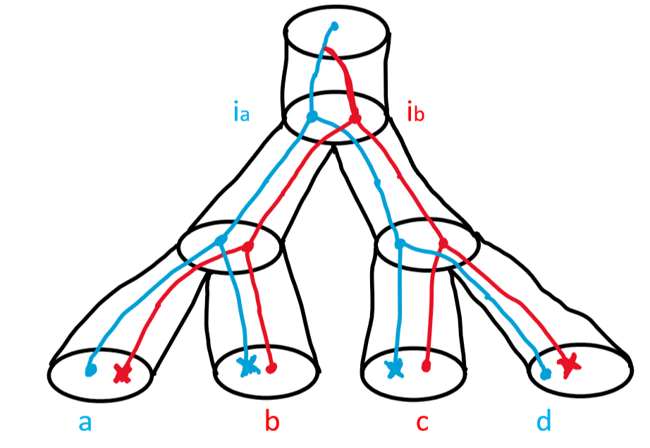
Figure 4: A realization of the GDL process on the balanced species tree $((A,B),(C,D))$ with ancestral copies. The sampled copies are named $a,b,c,d$, respectively in the figure. The left (blue) copy of $A$ was selected, so it is labeled $a$. It descends from node $i_{a}$ at $I$. Similarly, the right (red) copy of $B$ was selected, was labeled $b$, and descended from node $i_{b}$ at $I$. The figure shows that $a$ and $d$ descend from the same individual at $I$, which is expressed as $i_{a}=i_{d}$. Similarly, $i_{b}=i_{c}$ holds.

Letting $x=\mathbf{P}^{\prime}_{N_{I}}(i_{a}=i_{b})$ and $y=\mathbf{P}^{\prime}_{N_{I}}(i_{c}=i_{d})$, we define $h_{w}(x,y)$ to be the probability of the $w$th topology as follows. Let $w=1$ correspond to the species tree topology. Let $w=2$ correspond to either of the two alternative balanced topologies, which have the same probability by exchangeability of sibling species. Let $w=3$ correspond to any of the four caterpillar topologies in which the cherry is $\{a,b\}$. Let $w=4$ correspond to any of the caterpillar topologies in which the cherry is $\{c,d\}$. Let $w=5$ correspond to any of the remaining eight caterpillar topologies.

The main result of this section is that the species tree topology has the maximal probability. This is similar to what is found in MSC.

Theorem 2.

Let $\sigma$ be a species tree on four species $A,B,C,D$ with the balanced topology. Then $\mathbf{P}(u(t)=\mathcal{T})$ is maximized when $\mathcal{T}$ corresponds to the species tree topology.

To prove the result, we write explicit formulas for these probabilities.

Proposition 1.

(i) The balanced topologies have the following probabilities:

$$h_{1}(x,y) =xy+\left(x(1-y)+(1-x)y\right)\frac{N_{I}-2}{3N_{I}}\mathbf{1}(N_{I}\geq 3)$$

$$+(1-x)(1-y)\frac{\begin{pmatrix}N_{I}\\ 2\end{pmatrix}-2(N_{I}-1)+1}{9\begin{pmatrix}N_{I}\\ 2\end{pmatrix}}\mathbf{1}(N_{I}\geq 4).$$

$$h_{2}(x,y) =(1-x)(1-y)\bigg{[}\bigg{(}\frac{1}{N_{I}(N_{I}-1)}+\frac{N_{I}-1}{3\begin{pmatrix}N_{I}\\ 2\end{pmatrix}}\bigg{)}\mathbf{1}(N_{I}\geq 2)$$

$$+\frac{\begin{pmatrix}N_{I}\\ 2\end{pmatrix}-2(N_{I}-1)+1}{9\begin{pmatrix}N_{I}\\ 2\end{pmatrix}}\mathbf{1}(N_{I}\geq 4)\bigg{]}.$$

The caterpillar topologies have the following probabilities:

$$h_{3}(x,y) =x(1-y)\bigg{[}\frac{1}{N_{I}}\mathbf{1}(N_{I}\geq 2)+\frac{N_{I}-2}{3N_{I}}\mathbf{1}(N_{I}\geq 3)\bigg{]}$$

$$+(1-x)(1-y)\frac{\begin{pmatrix}N_{I}\\ 2\end{pmatrix}-2(N_{I}-1)+1}{18\begin{pmatrix}N_{I}\\ 2\end{pmatrix}}\mathbf{1}(N_{I}\geq 4)$$

$$h_{4}(x,y) =(1-x)y\bigg{[}\frac{1}{N_{I}}\mathbf{1}(N_{I}\geq 2)+\frac{N_{I}-2}{3N_{I}}\mathbf{1}(N_{I}\geq 3)\bigg{]}$$

$$+(1-x)(1-y)\frac{\begin{pmatrix}N_{I}\\ 2\end{pmatrix}-2(N_{I}-1)+1}{18\begin{pmatrix}N_{I}\\ 2\end{pmatrix}}\mathbf{1}(N_{I}\geq 4)$$

$$h_{5}(x,y) =(1-x)(1-y)\left(\frac{N_{I}-2}{3N_{I}(N_{I}-1)}\mathbf{1}(N_{I}\geq 3)+\frac{\begin{pmatrix}N_{I}\\ 2\end{pmatrix}-2(N_{I}-1)+1}{18\begin{pmatrix}N_{I}\\ 2\end{pmatrix}}\mathbf{1}(N_{I}\geq 4)\right).$$

Proof.

The proof is a basic application of the law of total probability and counting Legried et al. (2021), Hill et al. (2022). ∎

The next Propositions provide a ranking of probabilities that hold for any $N_{I}$ and when $x,y\geq 1/N_{I}$.

Proposition 2.

Suppose $x,y\geq 1/N_{I}$. Then $h_{1}(x,y)\geq h_{2}(x,y)\geq h_{5}(x,y)$.

Proof.

We start by showing $h_{1}\geq h_{2}$. The difference is

$$h_{1}(x,y)-h_{2}(x,y) =xy+\left(x(1-y)+(1-x)y\right)\frac{N_{I}-2}{3N_{I}}\mathbf{1}(N_{I}\geq 3)$$

$$-(1-x)(1-y)\frac{2N_{I}-1}{3N_{I}(N_{I}-1)}\mathbf{1}(N_{I}\geq 2).$$

When taking the partial derivative in $x$, we split $1-2y$ into $1-y-y$. Then the partial derivative in $x$ is

$$y+(1-2y)\frac{N_{I}-2}{3N_{I}}\mathbf{1}(N_{I}\geq 3)+(1-y)\frac{2N_{I}-1}{3N_{I}(N_{I}-1)}\mathbf{1}(N_{I}\geq 2)$$

$$=y\left(1-\frac{N_{I}-2}{3N_{I}}\mathbf{1}(N_{I}\geq 3)\right)+(1-y)\left(\frac{N_{I}-2}{3N_{I}}\mathbf{1}(N_{I}\geq 3)+\frac{2N_{I}-1}{3N_{I}(N_{I}-1)}\mathbf{1}(N_{I}\geq 2)\right)$$

The same holds when we compute the partial derivative in $y$. The function $h_{1}-h_{2}$ is linear in both $x$ and $y$, so the minimum value of $h_{1}-h_{2}$ is obtained by substituting $x=y=1/N_{I}$. Then

$$h_{1}(x,y)-h_{2}(x,y)\geq h_{1}(1/N_{I},1/N_{I})-h_{2}(1/N_{I},1/N_{I})=\begin{cases}1/N_{I}^{3}&N_{I}\geq 3\\ 1/N_{I}^{2}&N_{I}=1,2.\end{cases}$$

So $h_{1}\geq h_{2}$.

To show $h_{2}\geq h_{5}$, we only need to subtract. The difference is

$$h_{2}(x,y)-h_{5}(x,y)$$

$$=(1-x)(1-y)\bigg{(}\frac{5}{6}+\left(\frac{1}{N_{I}(N_{I}-1)}+\frac{2}{3N_{I}}-\frac{N_{I}-2}{3N_{I}(N_{I}-1)}\right)\mathbf{1}(N_{I}\geq 3)$$

$$+\frac{\begin{pmatrix}N_{I}\\ 2\end{pmatrix}-2(N_{I}-1)+1}{18\begin{pmatrix}N_{I}\\ 2\end{pmatrix}}\mathbf{1}(N_{I}\geq 4)\bigg{)}$$

$$=(1-x)(1-y)\bigg{(}\frac{5}{6}+\frac{N_{I}+3}{3N_{I}(N_{I}-1)}\mathbf{1}(N_{I}\geq 3)$$

$$+\frac{\begin{pmatrix}N_{I}\\ 2\end{pmatrix}-2(N_{I}-1)+1}{18\begin{pmatrix}N_{I}\\ 2\end{pmatrix}}\mathbf{1}(N_{I}\geq 4)\bigg{)},$$

which is clearly non-negative for all choices of $x$ and $y$. ∎

Proposition 3.

Suppose $x,y\geq 1/N_{I}$. Then $h_{1}(x,y)\geq h_{3}(x,y)\geq h_{5}(x,y)$.

Proof.

We start by showing that $h_{1}\geq h_{3}$. The difference is

$$h_{1}(x,y)-h_{3}(x,y) =xy+(1-x)y\frac{N_{I}-2}{3N_{I}}\mathbf{1}(N_{I}\geq 3)$$

$$-x(1-y)\frac{1}{N_{I}}\mathbf{1}(N_{I}\geq 2)$$

$$+(1-x)(1-y)\frac{\begin{pmatrix}N_{I}\\ 2\end{pmatrix}-2(N_{I}-1)+1}{18\begin{pmatrix}N_{I}\\ 2\end{pmatrix}}\mathbf{1}(N_{I}\geq 4).$$

The only negative part is in the second line, and it can be split into

$$-x(1-y)\frac{1}{N_{I}}\mathbf{1}(N_{I}\geq 2)=-x\frac{1}{N_{I}}\mathbf{1}(N_{I}\geq 2)+xy\frac{1}{N_{I}}\mathbf{1}(N_{I}\geq 2).$$

However, $y\geq 1/N_{I}$ and combining this negative term with the positive $xy$ term in the original expression implies

$$xy-x\frac{1}{N_{I}}\mathbf{1}(N_{I}\geq 2)\geq 0.$$

This dispenses with all negative terms, showing that $h_{1}\geq h_{3}$.

Now we show that $h_{3}\geq h_{5}$. The difference is

$$h_{3}(x,y)-h_{5}(x,y) =x(1-y)\bigg{[}\frac{1}{N_{I}}\mathbf{1}(N_{I}\geq 2)+\frac{N_{I}-2}{3N_{I}}\mathbf{1}(N_{I}\geq 3)\bigg{]}$$

$$-(1-x)(1-y)\frac{N_{I}-2}{3N_{I}(N_{I}-1)}\mathbf{1}(N_{I}\geq 3).$$

Using $x\geq 1/N_{I}$ implies

$$x(1-y)\bigg{[}\frac{1}{N_{I}}\mathbf{1}(N_{I}\geq 2)+\frac{N_{I}-2}{3N_{I}}\mathbf{1}(N_{I}\geq 3)\bigg{]}-(1-y)\frac{N_{I}-2}{3N_{I}(N_{I}-1)}\mathbf{1}(N_{I}\geq 3)\bigg{]}$$

$$\geq(1-y)\bigg{[}\frac{1}{2^{2}}+\frac{2N_{I}-1}{3N_{I}(N_{I}-1)}\mathbf{1}(N_{I}\geq 3)\bigg{]}\geq 0.$$

We have covered all negative components of $h_{3}-h_{5}$ with corresponding positive numbers, so we conclude $h_{3}\geq h_{5}$. ∎

Proposition 4.

Suppose $x,y\geq 1/N_{I}$. Then $h_{1}(x,y)\geq h_{4}(x,y)\geq h_{5}(x,y)$.

Proof.

The proof is identical to that of Proposition 3, except we switch the roles of $x$ and $y$. ∎

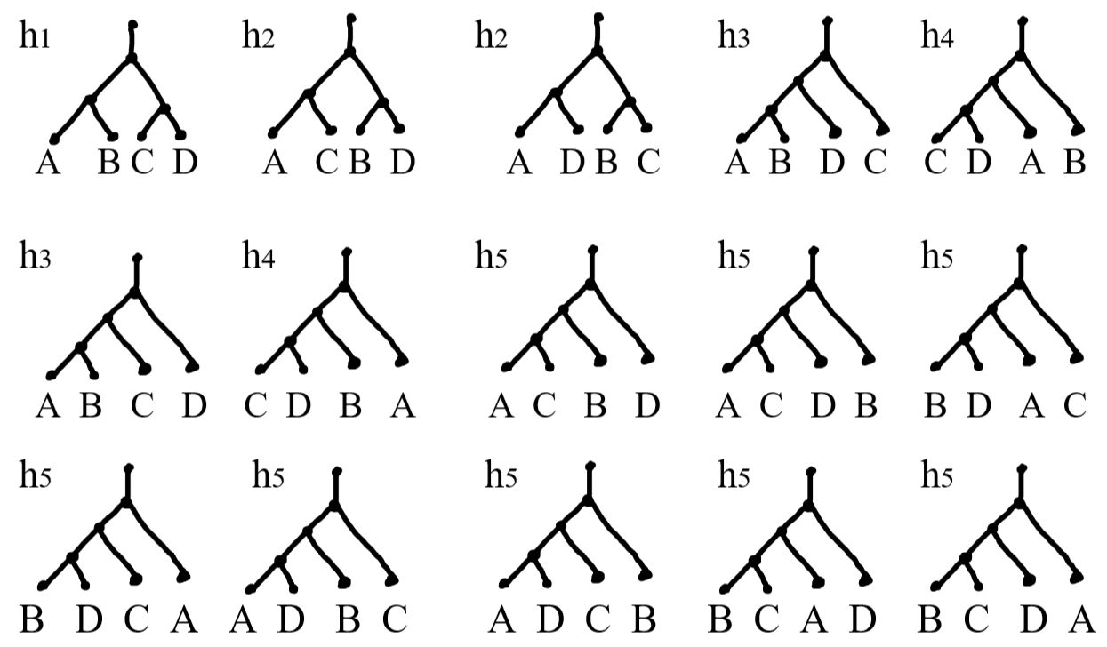
Figure 5: Labelling of the possible uniformly sampled gene trees by probability in the case of the balanced species tree.

5 Caterpillar topology on four leaves.

In this section, the species tree $\sigma$ is assumed to have four leaf species $A,B,C,$ and $D$ and the topology has $A,B$ are siblings, followed by $C$ as an outgroup, and followed by $D$ as a further outgroup. The Newick tree format is $(((A,B),C),D)$. The edge lengths are $s$ for the stem edge, $f$ for the parent edge to $A$ and $B$, $g$ for the parent edge to the most recent common ancestor of $A,B,$ and $C$, and $f_{n}^{\prime},n\in\{A,B,C,D\}$ for the lengths of the pendant edges incident to the leaves. The root vertex is labeled $I$, as in the previous sections. Let $\mathbf{P}^{\prime}$ be the probability measure subject to the conditioning event where $N_{A},N_{B},N_{C},$ and $N_{D}$ are positive. Let $I$ be the most recent common ancestor to the four species; $J$ be the most recent common ancestor to $A,B,C$; and $K$ be the most recent common ancestor to $A$ and $B$. The names of the ancestors of sampled copies are $k_{\ell},\ell\in\{a,b\}$; $j_{\ell^{\prime}},\ell^{\prime}\in\{a,b,c\}$; and $i_{\ell^{\prime\prime}},\ell^{\prime\prime}\in\{a,b,c,d\}$. Conditioning further on $N_{I}$, the probability of each gene tree topology is written using $N_{I}$, with the measure $\mathbf{P}^{\prime}_{N_{I}}$.

The main theorem of this section establishes possible anomaly zones for the caterpillar tree. Anomalous gene trees can correspond to only balanced quartets.

Theorem 3.

Let $\sigma$ be a species tree on four species $A,B,C,D$ with the caterpillar topology. Then $\mathbf{P}(u(t)=\mathcal{T})$ is maximized when $\mathcal{T}$ corresponds to either the species tree or one of the balanced rooted quartets.

Throughout, we let $k_{w^{\prime}}$ denote the probability of gene tree $t_{w^{\prime}}$, with $w^{\prime}$ indexed as follows. The species tree is listed first, followed by the possible anomalous gene trees. Let $k_{1}$ denote the probability of caterpillar tree $(((a,b),c),d)$, let $k_{2}$ denote the probability of the balanced tree $((a,b),(c,d)$, and let $k_{3}$ denote the probability of each alternate balanced tree $((a,c),(b,d))$ and $((a,d),(b,c))$. Then $k_{w^{\prime}},w^{\prime}\in\{4,5,...,8\}$ represent the other caterpillar topologies. It will be shown that $t_{2}$ has greater probability than $t_{3}$, implying three possible rankings of probability. They are (I) $k_{1}>k_{2}>k_{3}$ (no anomalous gene trees); (II) $k_{2}>k_{1}>k_{3}$ ($t_{2}$ is anomalous); and (III) $k_{2}>k_{3}>k_{1}$ (all balanced trees are anomalous).

The following Proposition gives the probability that the gene tree equals the species tree. Here, we first let $w=\mathbf{P}^{\prime}_{N_{I}}(j_{a}=j_{b})$ and $\\ x=\mathbf{P}^{\prime}_{N_{I}}(i_{a}=i_{b}=i_{c}|j_{a}=j_{b})$. Conditioned on $j_{a}\neq j_{b}$, we let

$$y=\mathbf{P}^{\prime}_{N_{I}}(i_{a}=i_{b}=i_{c},|\{j_{a},j_{b},j_{c}\}|=3|j_{a}\neq j_{b}).$$

From exchangeability of $j_{a}$ and $j_{b}$, we let

$$v=\mathbf{P}^{\prime}_{N_{I}}(i_{a}=i_{b}=i_{c},j_{a}=j_{c}|j_{a}\neq j_{b})=\mathbf{P}^{\prime}_{N_{I}}(i_{a}=i_{b}=i_{c},j_{b}=j_{c}|j_{a}\neq j_{b}).$$

From exchangeability of $i_{a},i_{b},i_{c}$ when $j_{a}\neq j_{c}$, we let

$$z=\mathbf{P}^{\prime}_{N_{I}}(i_{a}=i_{b}\neq i_{c}|j_{a}\neq j_{b})=\mathbf{P}^{\prime}_{N_{I}}(i_{a}=i_{c}\neq i_{b}|j_{a}\neq j_{b})=\mathbf{P}^{\prime}_{N_{I}}(i_{b}=i_{c}\neq i_{a}|j_{a}\neq j_{b}).$$

Before we proceed, we establish bounds on $w$ and $x$.

Lemma 1.

Conditioned on $N_{I}$, we have $w,x\geq\frac{1}{N_{I}}$.

Proof.

Both bounds follow mostly from Lemma 1 of Legried et al. (2021). The bound on $w$ follows by conditioning on $N_{K}$, the total number of individuals surviving to $K$. Letting $(M_{k})_{k=1}^{N_{I}}$ be the descendants of each individual at $I$ surviving to $K$, the selection of $j_{a}$ and $j_{b}$ are independent. We have

$$w=\mathbf{P}^{\prime}_{N_{K}}(j_{a}=j_{b}) =\mathbf{E}^{\prime}_{N_{I}}\left[\frac{\sum_{k=1}^{N_{I}}M_{k}^{2}}{(\sum_{k=1}^{N_{I}}M_{k})^{2}}\bigg{|}(M_{k})_{k=1}^{N_{I}}\right]$$

$$\geq\mathbf{E}^{\prime}_{N_{I}}\left[\frac{1}{N_{I}}\right]=\frac{1}{N_{I}}.$$

The inequality utilized is the quadratic mean inequality.

Now we consider the bound on $x$. Conditioned on $j_{a}=j_{b}$, the event $i_{a}=i_{b}$ is known to occur. So $x=\mathbf{P}^{\prime}_{N_{I}}(i_{a}=i_{c}|j_{a}=j_{b})$. Letting $(M_{j})_{j=1}^{N_{I}}$ be the descendants of each individual at $I$ surviving to $J$, the selection of $j_{a}$ and $j_{c}$ are proportional to these weights and are independent. Then

$$\mathbf{P}^{\prime}_{N_{I}}(i_{a}=i_{c}|j_{a}=j_{b}) =\mathbf{E}^{\prime}_{N_{I}}\left[\frac{\sum_{j=1}^{N_{I}}M_{j}^{2}}{\left(\sum_{j=1}^{N_{I}}M_{j}\right)^{2}}\bigg{|}(M_{j})_{j=1}^{N_{I}}\right],$$

and we obtain the lower bound of $1/N_{I}$. ∎

The next lemma follows similarly by considering the case where $i_{a}=i_{b}=i_{c}$.

Lemma 2.

Conditioned on $N_{I}$, we have $wx\geq(1-w)v$.

Proof.

We have

$$wx =\mathbf{P}^{\prime}_{N_{I}}(i_{a}=i_{b}=i_{c},j_{a}=j_{b})$$

$$(1-w)v =\mathbf{P}^{\prime}_{N_{I}}(i_{a}=i_{b}=i_{c},j_{a}=j_{c}\neq j_{c}).$$

Then

$$wx-(1-w)v$$

$$=\left(\mathbf{P}^{\prime}_{N_{I}}(j_{a}=j_{b}|i_{a}=i_{b}=i_{c})-\mathbf{P}^{\prime}_{N_{I}}(j_{a}=j_{c}\neq j_{b}|i_{a}=i_{b}=i_{c})\right)\mathbf{P}^{\prime}_{N_{I}}(i_{a}=i_{b}=i_{c}).$$

The factor contained in the parentheses through a similar method to Lemma 1. ∎

Proposition 5.

The caterpillar topology $(((a,b),c),d)$ has the probability

$$k_{1} =wx+w(1-x)\left(1-\frac{2}{N_{I}}\right)\frac{1}{3}\mathbf{1}(N_{I}\geq 3)$$

$$+(1-w)y\frac{1}{3}+(1-w)z\left(1-\frac{2}{N_{I}}\right)\frac{1}{3}\mathbf{1}(N_{I}\geq 3)$$

$$+(1-w)(1-y{\color[rgb]{0,0,0}-2v}-3z)\left(1-\frac{3}{N_{I}}\right)\frac{1}{18}\mathbf{1}(N_{I}\geq 4).$$

Proof.

This follows from the law of total probability. Note that when $i_{a},i_{b},i_{c},i_{d}$ are distinct, the probability of the correct caterpillar topology is $1/18$. ∎

Next, let $k_{2}$ be the probability of the balanced topology $((a,b),(c,d))$ and $k_{3}$ be the probability of the alternate balanced topology $((a,c),(b,d))$. Exchangeability of $a$ and $b$ means that $((a,d),(b,c))$ also has probability $k_{3}$.

Proposition 6.

The balanced topology $((a,b),(c,d))$ has probability

$$k_{2} =w(1-x)\left[\frac{1}{N_{I}}\mathbf{1}(N_{I}\geq 2)+\left(1-\frac{2}{N_{I}}\right)\frac{1}{3}\mathbf{1}(N_{I}\geq 3)\right]$$

$$+(1-w)z\left[\frac{1}{N_{I}}\mathbf{1}(N_{I}\geq 2)+\left(1-\frac{2}{N_{I}}\right)\frac{1}{3}\mathbf{1}(N_{I}\geq 3)\right]$$

$$+(1-w)(1-y{\color[rgb]{0,0,0}-2v}-3z)\left[\frac{1}{3}\frac{1}{N_{I}}\mathbf{1}(N_{I}\geq 3)+\left(1-\frac{3}{N_{I}}\right)\frac{1}{9}\mathbf{1}(N_{I}\geq 4)\right].$$

The balanced topology $((a,c),(b,d))$ has probability

$$k_{3} =(1-w)z\left[\frac{1}{N_{I}}\mathbf{1}(N_{I}\geq 2)+\left(1-\frac{2}{N_{I}}\right)\frac{1}{3}\mathbf{1}(N_{I}\geq 3)\right]$$

$$+(1-w)(1-y{\color[rgb]{0,0,0}-2v}-3z)\left[\frac{1}{3}\frac{1}{N_{I}}\mathbf{1}(N_{I}\geq 3)+\left(1-\frac{3}{N_{I}}\right)\frac{1}{9}\mathbf{1}(N_{I}\geq 4)\right].$$

Now, we consider caterpillar topologies where the unrooted topology is the same as the species tree. Let $k_{4}$ be the probability of $(((a,b),d),c)$ and $k_{5}$ be the probability of $(((c,d),a),b)$. The topology $(((c,d),b),a)$ has the same probability $k_{5}$.

Proposition 7.

The caterpillar topology $(((a,b),d),c)$ has probability

$$k_{4} =w(1-x)\left[\frac{1}{N_{I}}\mathbf{1}(N_{I}\geq 2)+\left(1-\frac{2}{N_{I}}\right)\frac{1}{3}\mathbf{1}(N_{I}\geq 3)\right]$$

$$+(1-w)z\left[\frac{1}{N_{I}}\mathbf{1}(N_{I}\geq 2)+\left(1-\frac{2}{N_{I}}\right)\frac{1}{3}\mathbf{1}(N_{I}\geq 3)\right]$$

$$+(1-w)(1-y-3z)\left(1-\frac{3}{N_{I}}\right)\frac{1}{18}\mathbf{1}(N_{I}\geq 4).$$

The caterpillar topology $(((c,d),a),b)$ has probability

$$k_{5} =(1-w)(1-y{\color[rgb]{0,0,0}-2v}-3z)\left[\frac{1}{3}\frac{1}{N_{I}}\mathbf{1}(N_{I}\geq 3)+\left(1-\frac{3}{N_{I}}\right)\frac{1}{18}\mathbf{1}(N_{I}\geq 4)\right].$$

Lastly, we consider four caterpillar topologies where the unrooted topology is $((a,c),(b,d))$. Let $k_{6}$ be the probability of $(((a,c),b),d)$, $k_{7}$ be the probability of $(((a,c),d),b)$, $k_{8}$ be the probability of $(((b,d),a),c)$, and $k_{9}$ be the probability of $(((b,d),c),a)$. The other caterpillar topologies with unrooted topology $((a,d),(b,c))$ are represented in this calculation.

Proposition 8.

The caterpillar topology $(((a,c),b),d)$ has probability

$$k_{6} ={\color[rgb]{0,0,0}(1-w)v}+(1-w)y\frac{1}{3}+(1-w)z\left(1-\frac{2}{N_{I}}\right)\frac{1}{3}\mathbf{1}(N_{I}\geq 3)$$

$$+(1-w)(1-y{\color[rgb]{0,0,0}-2v}-3z)\left(1-\frac{3}{N_{I}}\right)\frac{1}{18}\mathbf{1}(N_{I}\geq 4).$$

The caterpillar topology $(((a,c),d),b)$ has probability

$$k_{7} =(1-w)z\left[\frac{1}{N_{I}}\mathbf{1}(N_{I}\geq 2)+\left(1-\frac{2}{N_{I}}\right)\frac{1}{3}\mathbf{1}(N_{I}\geq 3)\right]$$

$$+(1-w)(1-y{\color[rgb]{0,0,0}-2v}-3z)\left[\frac{1}{3}\frac{1}{N_{I}}\mathbf{1}(N_{I}\geq 3)+\left(1-\frac{3}{N_{I}}\right)\frac{1}{18}\mathbf{1}(N_{I}\geq 4)\right].$$

The caterpillar topologies $(((b,d),a),c)$ and $(((b,d),c),a)$ have probability

$$k_{8} =(1-w)(1-y{\color[rgb]{0,0,0}-2v}-3z)\left[\frac{1}{3}\frac{1}{N_{I}}\mathbf{1}(N_{I}\geq 3)+\left(1-\frac{3}{N_{I}}\right)\frac{1}{18}\mathbf{1}(N_{I}\geq 4)\right].$$

We now rank these probabilities where possible and determine when the average $k_{1}$ is not the maximal probability.

Proposition 9.

We have $k_{1}\geq k_{4},k_{5},k_{6},k_{7},k_{8}$.

Proof.

For $k_{1}\geq k_{4}$, we eliminate the non-corresponding terms. This leaves

$$k_{1}-k_{4} =wx+(1-w)y\frac{1}{3}-\left[w(1-x)+(1-w)z\right]\frac{1}{N_{I}}\mathbf{1}(N_{I}\geq 2).$$

Because $x\geq\frac{1}{N_{I}}$, we have

$$wx-w(1-x)\frac{1}{N_{I}}\mathbf{1}(N_{I}\geq 2) =w\left[x\left(1+\frac{1}{N_{I}}\mathbf{1}(N_{I}\geq 2)\right)-\frac{1}{N_{I}}\mathbf{1}(N_{I}\geq 2)\right]$$

$$\geq\frac{w}{N_{I}}$$

Because $w\geq\frac{1}{N_{I}}$, we have

$$\frac{w}{N_{I}}-(1-w)z\frac{1}{N_{I}}\mathbf{1}(N_{I}\geq 2) =w\left(\frac{1}{N_{I}}+z\frac{1}{N_{I}}\mathbf{1}(N_{I}\geq 2)\right)-z\frac{1}{N_{I}}\mathbf{1}{N_{I}\geq 2}$$

$$\geq\frac{1}{N_{I}^{2}}.$$

This covers all the negative terms, so $k_{1}\geq k_{4}$, as needed.

We now show $k_{1}\geq k_{5}$. We first observe that

$$wx+w(1-x)\left(1-\frac{2}{N_{I}}\right)\frac{1}{3}\mathbf{1}(N_{I}\geq 3)=\frac{w}{3}\left(1-\frac{2}{3N_{I}}+\frac{2x}{3}\right)\geq\frac{1}{3N_{I}}.$$

This is at least

$$(1-w)(1-y{\color[rgb]{0,0,0}-2v}-3z)\frac{1}{3N_{I}},$$

which is sufficient to conclude $k_{1}\geq k_{5}$ by cancelling other terms of $k_{5}$.

That $k_{1}\geq k_{6}$ follows directly from Lemma 2. The remaining claims follow by cancelling terms and using the inequality from the previous paragraph. ∎

We also have that $k_{2}\geq k_{3}$, which is apparent. This establishes the trichotomy stated in Theorem 3.

Proposition 10.

We have $k_{2}\geq k_{3}$.

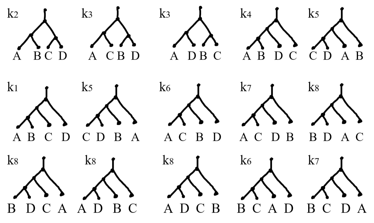
Figure 6: Labelling of the possible uniformly sampled gene trees by probability in the case of the caterpillar species tree.

5.1 Existence of anomaly zones

In this subsection, we consider some cases where anomaly zones arise. Under MSC, this amounts to choosing a caterpillar species tree with small enough branch lengths. In this paper, we consider branch lengths as well as the birth rate $\lambda$.

Let $\eta_{I}$ be the length of the interior child edge of $I$ and $\eta_{J}$ be the length of the interior child edge of $J$. Provided $\eta_{I}$ and $\eta_{J}$ are sufficiently small, there is an anomaly zone for some choices of $\lambda$ and $\mu$. The explicit formulas are described in this section, and we provide figures to display the results.

Theorem 4.

Let $\sigma=(\mathcal{T},\mathbf{f})$ be a species tree on four species $A,B,C,D$ with the caterpillar topology $\mathcal{T}$ and let $\mu$ be fixed Then as $\eta_{I}$ and $\eta_{J}$ converge to $0$, there exist positive rates $\lambda$ such that $\mathbf{P}^{\prime}(u(t)=\mathcal{T}^{\prime})>\mathbf{P}^{\prime}(u(t)=\mathcal{T})$ when $\mathcal{T}^{\prime}$ is any choice of balanced topology joining the uniformly sampled copies $a,b,c,d$.

Before establishing the Theorem, we first prove the convergence of $w,x,y,z$ in these limits.

Proposition 11.

Let $N_{I}$ and $w,x,y,z$ be defined as before. Then as $\eta_{I},\eta_{J}\rightarrow 0$, we have

$$w,x\rightarrow\frac{1}{N_{I}}\ \textnormal{and}\ (1-w)v,y,z\rightarrow 0.$$

Proof.

As $\eta_{I}\rightarrow 0$, we have the offspring numbers $(M_{j})_{j=1}^{N_{I}}$ each converge to $1$ in distribution as $\eta_{I}\rightarrow 0$. Because the $M_{j}$ are independent, the vector $(M_{1},...,M_{I})$ converges in distribution to the vector $(1,...,1)$ as $\eta_{I}\rightarrow 0$. The function $\mathcal{F}(y_{1},...,y_{N_{I}})=\sum_{j=1}^{N_{I}}y_{j}^{2}/(\sum_{j=1}^{N_{I}}y_{j})^{2}$ is bounded and continuous around $(1,...,1)$, so the Portmanteau Theorem implies that

$$\mathbf{E}^{\prime}_{N_{I}}[\mathcal{F}(M_{1}(\eta_{I}),...,M_{I}(\eta_{I}))\rightarrow\mathbf{E}^{\prime}_{N_{I}}[\mathcal{F}(M_{1}(0),...,M_{N_{I}}(0))]=\frac{1}{N_{I}}$$

as $\eta_{I}\rightarrow 0$. For the connections in probability, see Durrett (2010).

Conditioned on $j_{a}=j_{b}$, the event $i_{a}=i_{c}$ is equivalent to the coalescence of a single independent pair, i.e. $x\rightarrow 1/N_{I}$ as $\eta_{I}\rightarrow 0$. A similar conclusion holds for $w\rightarrow 1/N_{I}$ as both $\eta_{I},\eta_{J}$ tend to $0$. In the event that $j_{a}\neq j_{b}$, it is not possible for $i_{a}=i_{b}$ as $\eta_{I}\rightarrow 0$, so $(1-w)v,y,z\rightarrow 0$. ∎

Next, we consider the differences between $k_{1},k_{2},k_{3}$ in the case where $\eta_{I}$ and $\eta_{J}$ are in the limiting case of $0$. We have

$$k_{1} \rightarrow\frac{1}{N_{I}^{2}}+\frac{1}{N_{I}}\left(1-\frac{1}{N_{I}}\right)\left(1-\frac{2}{N_{I}}\right)\frac{1}{3}\mathbf{1}(N_{I}\geq 3)$$

$$+\left(1-\frac{1}{N_{I}}\right)\left(1-\frac{3}{N_{I}}\right)\frac{1}{18}\mathbf{1}(N_{I}\geq 4)$$

$$k_{2} \rightarrow\frac{1}{N_{I}}\left(1-\frac{1}{N_{I}}\right)\left[\frac{1}{N_{I}}\mathbf{1}(N_{I}\geq 2)+\left(1-\frac{2}{N_{I}}\right)\frac{1}{3}\mathbf{1}(N_{I}\geq 3)\right]$$

$$+\left(1-\frac{1}{N_{I}}\right)\left[\frac{1}{3}\frac{1}{N_{I}}\mathbf{1}(N_{I}\geq 3)+\left(1-\frac{3}{N_{I}}\right)\frac{1}{9}\mathbf{1}(N_{I}\geq 4)\right]$$

$$k_{3} \rightarrow\left(1-\frac{1}{N_{I}}\right)\left[\frac{1}{3}\frac{1}{N_{I}}\mathbf{1}(N_{I}\geq 3)+\left(1-\frac{3}{N_{I}}\right)\frac{1}{9}\mathbf{1}(N_{I}\geq 4)\right].$$

The differences are

$$k_{1}-k_{2} =\begin{cases}1&\textnormal{if}\ N_{I}=1\\ \frac{3}{8}&\textnormal{if}\ N_{I}=2\\ \frac{1}{27}&\textnormal{if}\ N_{I}=3\\ \frac{1}{N_{I}^{3}}+\frac{1}{6N_{I}^{2}}-\frac{1}{9N_{I}}-\frac{1}{18}&\textnormal{if}\ N_{I}\geq 4,\end{cases}$$

$$k_{1}-k_{3} =\begin{cases}1&\textnormal{if}\ N_{I}=1\\ \frac{1}{4}&\textnormal{if}\ N_{I}=2\\ \frac{5}{81}&\textnormal{if}\ N_{I}=3\\ \frac{2}{3N_{I}^{3}}+\frac{1}{6N_{I}^{2}}+\frac{2}{9N_{I}}-\frac{1}{18}&\textnormal{if}\ N_{I}\geq 4.\end{cases}$$

To prove the Theorem, we observe Proposition 11 and compute the boundary of the anomaly zone by computing $\mathbf{E}^{\prime}[k_{1}-k_{2}]$ and $\mathbf{E}^{\prime}[k_{1}-k_{3}]$ using the modified geometric distribution of $N_{I}$ described in Section 3. First, in the limit as $\eta_{I}$ and $\eta_{J}$ converge to $0$, the topology of the tree is essentially a star tree. We first compute the probability that each species has at least one surviving gene copy.

Proposition 12.

In the limit as $\eta_{I}$ and $\eta_{J}$ converge to $0$, the unconditional survival probability converges to

$$e^{-(\lambda-\mu)s}(1-p_{0}(s))^{2}\left\{\frac{\alpha^{4}}{1-\alpha^{4}\beta}-4\frac{\alpha^{3}}{1-\alpha^{3}\beta}+6\frac{\alpha^{2}}{1-\alpha^{2}\beta}-4\frac{\alpha}{1-\alpha\beta}+\frac{1}{1-\beta}\right\},$$

where $\alpha=\frac{\mu}{\lambda}q(h)$ and $\beta=q(s).$

Proof.

Given $N_{I}=n$, the probability that $N_{A}=0$ is $\left[\frac{\mu}{\lambda}q(h)\right]^{n}$. That $N_{A},N_{B},N_{C},N_{D}$ are independent conditioned on $N_{I}$ implies the probability of survival given $N_{I}=n$ is

$$\left(1-\left[\frac{\mu}{\lambda}q(h)\right]^{n}\right)^{4}.$$

By the law of total probability, we have the unconditional probability of survival is

$$\sum_{n=1}^{\infty}\left(1-\left[\frac{\mu}{\lambda}q(h)\right]^{n}\right)^{4}\mathbf{P}(N_{I}=n)=e^{-(\lambda-\mu)s}(1-p_{0}(s))^{2}\sum_{n=1}^{\infty}\left(1-\left[\frac{\mu}{\lambda}q(h)\right]^{n}\right)^{4}q(s)^{n-1}.$$

Inside the series on the right-hand side, we expand to obtain summands of the form

$$\beta^{-1}\left\{(\alpha^{4}\beta)^{n}-4(\alpha^{3}\beta)^{n}+6(\alpha^{2}\beta)^{n}-4(\alpha\beta)^{n}+\beta^{n}\right\}.$$

The result follows by summing the many geometric series. ∎

Proof of Theorem 4.

The difference in probabilities is

$$\frac{e^{-(\lambda-\mu)s}(1-p_{0}(s))^{2}}{\mathbf{P}(N_{A},N_{B},N_{C},N_{D}>0)}\sum_{n=1}^{\infty}(k_{1}-k_{j})(n)(1-\alpha^{n})^{4}\beta^{n-1},j=2,3.$$

As $\lambda\rightarrow+\infty$, we find that $\alpha\rightarrow 0$ and $\beta\rightarrow 1$, so $\mathbf{P}(N_{A},N_{B},N_{C},N_{D}>0)\rightarrow 1$. It remains to check whether the series is negative for sufficiently large $\lambda$. For all $n\geq 4$, we have

$$\frac{1}{n^{3}}+\frac{1}{6n^{2}}-\frac{1}{9n}-\frac{1}{18}\leq-\frac{11}{192},$$

so the series is bounded above by

$$(1-\alpha^{4})+\frac{3}{8}(1-\alpha^{2})\beta+\frac{1}{27}(1-\alpha^{3})^{4}\beta^{2}-\frac{11}{192}\sum_{n=4}^{\infty}(1-\alpha^{n})^{4}\beta^{n-1}.$$ (1)

Similarly to the proof of Proposition 12, the series sums to

$$\frac{\alpha^{16}\beta^{3}}{1-\alpha^{4}\beta}-4\frac{\alpha^{12}\beta^{3}}{1-\alpha^{3}\beta}+6\frac{\alpha^{8}\beta^{3}}{1-\alpha^{2}\beta}-4\frac{\alpha^{4}\beta^{3}}{1-\alpha\beta}+\frac{\beta^{3}}{1-\beta}.$$

As $\lambda$ goes to $+\infty$, the expression in (1) converges to $-11/192$. It follows then that $\mathbf{E}^{\prime}[k_{1}-k_{2}]$ is bounded above by a function that is negative for sufficiently large $\lambda$, finding a zone where $((a,b),(c,d))$ has greater probability than the species topology.

For $k_{1}-k_{3}$ given $N_{I}$, we note that $k_{1}-k_{3}$ remains positive until $N_{I}$ is at least $6$. For $n\geq 6$, we have

$$\frac{2}{n^{3}}+\frac{1}{6n^{2}}+\frac{2}{9n}-\frac{1}{18}\leq-\frac{7}{648}.$$

Repeating the steps in the previous case shows there is $\lambda$ sufficiently large to provide a zone where $((a,c),(b,d))$ also has greater probability than the species topology. This completes the proof of the Theorem. ∎

5.2 Computational results

We plot the expected values of $k_{1}-k_{2}$ and $k_{1}-k_{3}$ for critical $\lambda$ in two cases of $\mu$ in the case where $\eta_{I}=\eta_{J}=0$ with specific settings for the weights of the root and pendant edges, see Figure 7. Proposition 10 and Theorem 4 are both apparent from these results. Notably, $\lambda$ must be quite large relative to $\mu$ to obtain an anomaly zone.

The results in Figure 7 show that anomaly zones of types (II) and (III) can be found for some settings of branch lengths in the case where $\mathcal{T}$ has the rooted caterpillar topology. Case (I) of no anomaly zone occurs in the lower left region (left and below the left curve); Case (II) where $((a,b),(c,d))$ has maximal probability occurs in the middle region but the species tree has the second highest probability; and Case (III) where all balanced topologies have higher probability than the species tree. Relative to the net speciation rate $\lambda-\mu$, the width of the regions associated to (II) are quite narrow.

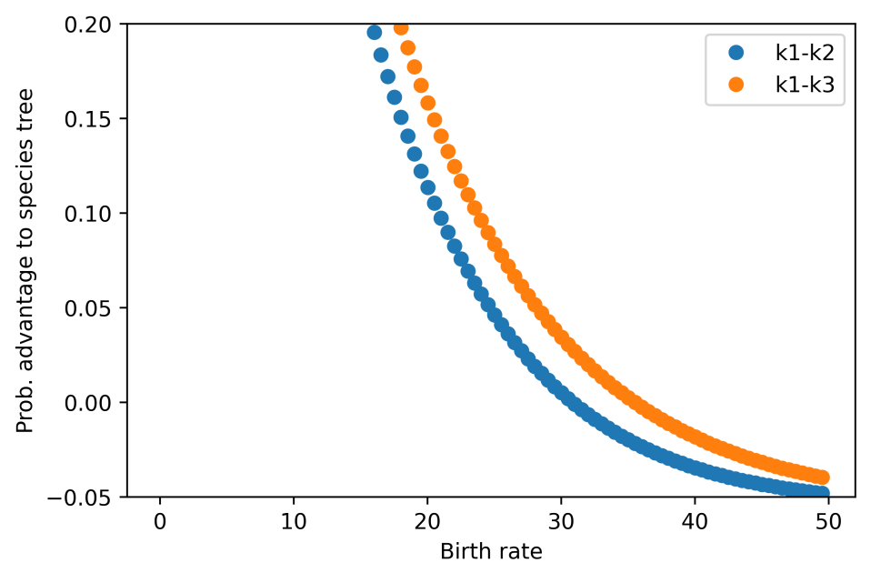
(a) label 1

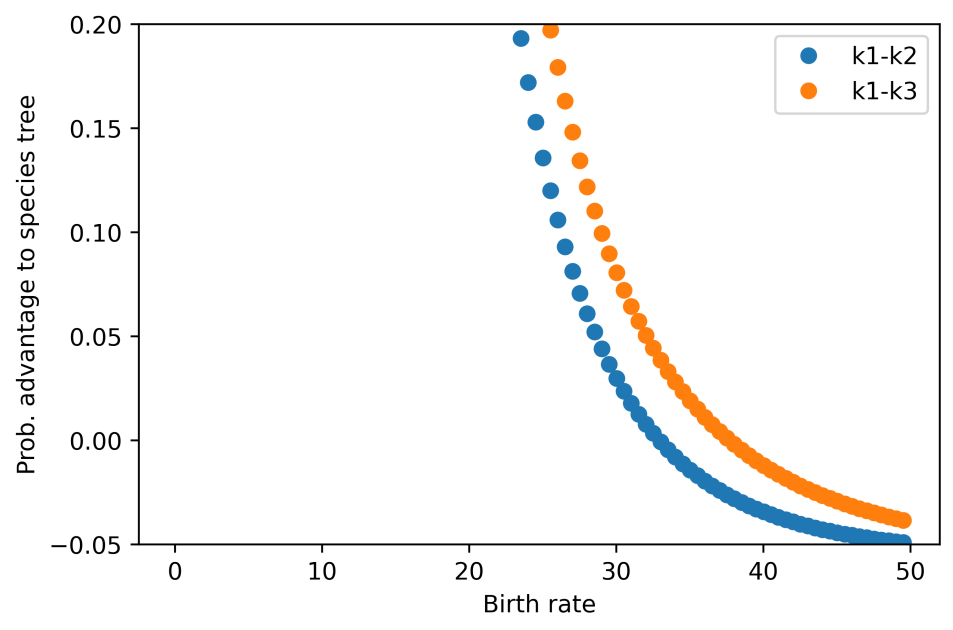
(b) label 2

Figure 7: (a) Expected values of $k_{1}-k_{2}$ and $k_{2}-k_{3}$ in the case of death rate $\mu=0.01$, root edge of length $0.01$, and leaf edges all length $0.05$. (b) Same settings as in (a), except the death rate is $\mu=3$.

6 Conclusion

Through more careful counting and bounding compared to previous efforts in this area, we showed that rooted balanced species quartets have no anomaly zones. We also showed that if anomaly zones exist, we have shown the respective anomalous gene trees must be balanced quartets. Moreover, the rooted caterpillar topology on four leaves has branch length settings, provided the birth rate is sufficiently large. As with the MSC, anomalous gene trees occur when both the interior branch lengths approach $0$.

This analysis shows that GDL could have similar issues with gene tree discordance as has been observed with MSC, but the structural information contained in the species tree might be more easily ascertained. This is because the branching events at speciation points must always occur. Because of possible anomalous gene trees provided in Theorem 3, it should be expected that this problem only becomes harder as more species are added to the tree. However, the analysis gets out of hand quickly as more gene trees are possible. It should be expected that only experimental or simulation evidence is practical to obtain in the case of larger trees.

Because the bounds obtained in Sections 5 and 6 utilize only the numbers of copies at particular points in the tree, it should be expected that the results of this paper and those of, e.g. Legried et al. (2021); Markin and Eulenstein (2021), etc. generalize to the case where birth and death rates are taken to vary over time or across edges in the species tree. There are practical issues raised about how to estimate the rate parameters from data Louca and Pennell (2020), Legried and Terhorst (2022), and Legried and Terhorst (2023). The difficulties raised there do not translate here.

The analysis of uniformly sampled gene trees as inputs to ASTRAL-one is already complicated, but that does not imply similar difficulties will appear with ASTRAL-multi, Rabiee et al. (2019). In ASTRAL-multi, the multi-labelled gene tree is instead replaced with a singly-labelled gene tree for every choice of species in the gene tree. The dependencies between same-labelled individuals in a gene tree make analysis seem daunting, but one advantage of ASTRAL-multi is that there is no need to condition on survival of all species. A disadvantage of conditioning on a present-day observation is that it induces a survivorship bias that can be difficult to model. In this paper, we engaged in analysis that avoids having to consider this bias. Another possibility is to analyze the distribution of pseudoorthologs only, see Smith and Hahn (2022). This approach would require new methods, as the conditional distribution seems more difficult to work with.

Lastly, the results of this paper suggest but do not give proof of existence of non-existence of anomaly zones under the DLCoal model Rasmussen and Kellis (2012). Rigorous proof would come through a more extensive analysis of the branching patterns than we can reasonably do here. It should be noted that even if balanced quartets have no anomaly zones, the resulting gene tree could have so many branches in it that the anomaly zone for the coalescence portion of the model is even larger than that of the simple MSC rooted quartet.

7 Acknowledgments

This work was completed in part while the author was a postdoctoral fellow at the Department of Statistics at the University of Michigan-Ann Arbor, in addition to their current position at the Georgia Institute of Technology. BL was supported by NSF grant DMS-1646108 and NSF-Simons grant for the Southeast Center for Mathematics and Biology DMS-1764406.

Appendix

Numbers of copies

The first two raw moments are easily computed by summing the geometric series. The first moment (the mean) is

$$\mathbf{E}[N_{s}] =e^{-(\lambda-\mu)s}\left(1-p_{0}(s)\right)^{2}\sum_{i=1}^{\infty}iq(s)^{i-1}$$

$$=e^{-(\lambda-\mu)s}\left(1-p_{0}(s)\right)^{2}\frac{1}{\left(1-q(s)\right)^{2}}$$

$$=e^{-(\lambda-\mu)s}\left(\frac{\lambda-\mu q(s)}{\lambda-\lambda q(s)}\right)^{2}.$$

The second moment is

$$\mathbf{E}[N_{s}^{2}] =e^{-(\lambda-\mu)s}\left(1-p_{0}(s)\right)^{2}\sum_{i=1}^{\infty}i^{2}q(s)^{i-1}$$

$$=e^{-(\lambda-\mu)s}\left(1-p_{0}(s)\right)^{2}\frac{1+q(s)}{\left(1-q(s)\right)^{3}}$$

$$=e^{-(\lambda-\mu)s}\frac{1+q(s)}{1-q(s)}\left(\frac{\lambda-\mu q(s)}{\lambda-\lambda q(s)}\right)^{2}.$$

The variance is then computed as

$$\textnormal{Var}[N_{s}]=\mathbf{E}[N_{s}^{2}]-\left(\mathbf{E}[N_{s}]\right)^{2}.$$

One may be interested in the conditional distribution of $N_{s}$, conditioned on non-extinction by time $s$, i.e. $N_{s}>0$. Because

$$\mathbf{P}(N_{s}>0)=1-\mathbf{P}(N_{s}=0)=1-p_{0}(s),$$

it follows for any $i>0$ that

$$\mathbf{P}(N_{s}=i|N_{s}>0)=\frac{\mathbf{P}(N_{s}=i)}{\mathbf{P}(N_{s}>0)}=e^{-(\lambda-\mu)s}\left(1-p_{0}(s)\right)q(s)^{i-1}.$$

So $N_{s}|N_{s}>0$ is a geometric random variable with success probability $1-q(s)$. The mean is

$$\mathbf{E}[N_{s}|N_{s}>0]=\frac{1}{1-q(s)}$$

and the variance is

$$\textnormal{Var}[N_{s}|N_{s}>0]=\frac{1+q(s)}{\left(1-q(s)\right)^{2}}-\frac{1}{\left(1-q(s)\right)^{2}}=\frac{q(s)}{\left(1-q(s)\right)^{2}}.$$

Next, the moment generating function can be used to compute some useful statistics. We have

$$M_{s}(\tau)=\mathbf{E}[e^{\tau N_{s}}] =\frac{\mu}{\lambda}q(s)+e^{-(\lambda-\mu)s}\left(1-p_{0}(s)\right)^{2}\sum_{i=0}^{\infty}e^{\tau i}q(s)^{i-1}$$

$$=\frac{\mu}{\lambda}q(s)+e^{-(\lambda-\mu)s}\left(1-p_{0}(s)\right)^{2}\frac{e^{\tau}}{1-q(s)e^{\tau}}$$

This function is defined for all $x$ such that $1-e^{\tau}q(s)>0$, which is an open neighborhood containing the origin.

The negative raw moments can also be computed. More generally, consider $N_{s}^{-P}e^{\tau N_{s}}$ for integers $P\geq 1$, conditioned on survival. The $P=1$ case has a closed-form expression:

$$\mathbf{E}\left[\frac{1}{N_{s}}e^{\tau N_{s}}|N_{s}>0\right] =e^{-(\lambda-\mu)s}\left(1-p_{0}(s)\right)\sum_{i=1}^{\infty}\frac{1}{i}q(s)^{i-1}$$

$$=e^{-(\lambda-\mu)s}\frac{1-p_{0}(s)}{q(s)}\int\sum_{i=1}^{\infty}q(s)^{i}\ dq(s)$$

$$=e^{-(\lambda-\mu)s}\frac{1-p_{0}(s)}{q(s)}\log\left(\frac{1}{1-q(s)e^{\tau}}\right).$$

For greater integers $P$, there is no closed form expression, but the well-known polylogarithm function can be used. It is defined as

$$\textnormal{Li}_{P}(\zeta)=\sum_{i=1}^{\infty}\frac{\zeta^{i}}{i^{P}}.$$

Then

$$\mathbf{E}\left[\frac{1}{N_{s}^{P}}e^{\tau N_{s}}|N_{s}>0\right]=e^{-(\lambda-\mu)s}\frac{1-p_{0}(s)}{q(s)}\textnormal{Li}_{P}\left(q(s)e^{\tau}\right).$$

Proof.

For the denominator on the left-hand side, we first start with the fact that $P^{-2}=\int_{\tau=0}^{\infty}\tau e^{-\tau P}\ d\tau$. Then

$$\frac{1}{\left(\sum_{j=1}^{N_{I}}N_{I,j}\right)^{2}}=\int_{\tau=0}^{\infty}\tau e^{-\tau\sum_{j=1}^{N_{I}}N_{I,j}}\ d\tau.$$

The $N_{I,j}$ are identically distributed, so

$$\mathbf{E}^{\prime}\left[\frac{\sum_{j=1}^{N_{I}}N_{I,j}^{2}}{\left(\sum_{j=1}^{N_{I}}N_{I,j}\right)^{2}}\bigg{|}N_{I}\right]=N_{I}\mathbf{E}^{\prime}\left[\frac{N_{I,1}^{2}}{\left(\sum_{j=1}^{N_{I}}N_{I,j}\right)^{2}}\bigg{|}N_{I}\right].$$

To utilize independence, we separate the $N_{I,1}$ factors from the others. We have

$$\mathbf{E}^{\prime}\left[\frac{N_{I,1}^{2}}{\left(\sum_{j=1}^{N_{I}}N_{I,j}\right)^{2}}\bigg{|}N_{I}\right]=\int_{\tau=0}^{\infty}\tau\mathbf{E}^{\prime}\left[N_{I,1}^{2}e^{-\tau N_{I,1}}|N_{I}\right]\mathbf{E}^{\prime}\left[e^{-\tau\sum_{j=2}^{N_{I}}N_{I,j}}|N_{I}\right]\ dx.$$

A couple basic properties of the moment generating function are that $M_{N,1}^{\prime\prime}(-\tau)=\mathbf{E}^{\prime}\left[N_{I,1}^{2}e^{-\tau N_{I,1}}\right]$ and $M_{N_{I,1}}(-\tau)^{N_{I}-1}=\prod_{j=2}^{N_{I}}\mathbf{E}^{\prime}[e^{-\tau N_{I,1}}|N_{I}]=\mathbf{E}^{\prime}[e^{-\tau\sum_{j=2}^{N_{I}}N_{I,j}}|N_{I}]$. Plugging these into the integral expression completes the proof. ∎

Other calculations for species trees on three leaves

Throughout this section, the species tree $\sigma=(\mathcal{T},\mathbf{f})$ is assumed to have three leaf species $A,B$, and $C$ and the topology has $A,B$ are siblings with $C$ as the outgroup. This rooted topology can be expressed using the Newick tree format: $((A,B),C)$. The edge lengths are $s$ for the stem edge, $f$ for the interior edge, and $g$ for the pendant edges incident to $A$ and $B$. The tree is ultrametric, so the pendant edge incident to $C$ has length $f+g$. The root vertex is labeled $I$, and the parent vertex to $A$ and $B$ is labeled $J$. For any vertex $v$ in the species tree, let $N_{v}$ be the size of the population. Our problem setting requires us to assume every contemporary species has at least one copy in a given gene tree, meaning $N_{A},N_{B},$ and $N_{C}$ are positive. An example of a possible gene tree is given in Figure 1. Let $\mathbf{P}^{\prime}$ be the probability measure subject to this conditioning. Expectations computed under the respective measures are denoted $\mathbf{E}$ and $\mathbf{E}^{\prime}$.

In Proposition 13, we give the transition probability for the continuous-time process $\{N_{s}\}_{s\geq 0}$.

Proposition 13.

Let $s,f>0$ so that $s$ and $s+f$ are successive times. Then

$$\mathbf{P}(N_{s+f}=j|N_{s}=i)=p_{j}(f)^{(\ast i)},$$

where $p_{j}(\cdot)^{(\ast i)}$ is the $i$-fold convolution of the function $p_{j}$.

Proof.

The progenies of the $i$ individuals at time $s$ are independent and identically distributed random variables, and $N_{s+f}$ is the sum. So $N_{s+f}$ has the same distribution as $\sum_{j=1}^{i}N_{f}$. The distribution of the independent and identically distributed summands is known to be the discrete convolution of $i$ copies of $p_{j}(\cdot)$ evaluated at $f$. ∎

In Proposition 14, we write the survival probability as an expectation over the numbers of copies at the internal nodes of $\mathcal{T}$.

Proposition 14.

We have

$$\mathbf{P}(N_{A},N_{B},N_{C}>0) =\mathbf{E}\left[\left(1-p_{0}(g)^{N_{J}}\right)^{2}\left(1-p_{0}(f+g)^{N_{I}}\right)\right]$$

$$=\mathbf{E}\left[\mathbf{E}\left[\left(1-p_{0}(g)^{N_{J}}\right)^{2}|N_{I}\right]\left(1-p_{0}(f+g)^{N_{I}}\right)\right].$$

Proof.

The second equality is immediate by the definition of conditional expectation. The rest of the proof is for the first equality. Condition on the specified values of $N_{I}$ and $N_{J}$. We first have $\mathbf{P}(N_{I}=i)=p_{i}(t)$ and $\mathbf{P}(N_{J}=j|N_{I}=i)=p_{\bullet}(f)$. The Markov property and conditional independence imply

$$\mathbf{P}(N_{A},N_{B},N_{C}>0)$$

$$=\sum_{i=1}^{\infty}\mathbf{P}(N_{A},N_{B},N_{C}>0|N_{I}=i)\mathbf{P}(N_{I}=i)$$

$$=\sum_{i=1}^{\infty}\mathbf{P}(N_{A},N_{B}>0|N_{I}=i)\mathbf{P}(N_{C}>0|N_{i}=i)\mathbf{P}(N_{I}=i)$$

$$=\sum_{i=1}^{\infty}\sum_{j=1}^{\infty}\mathbf{P}(N_{A},N_{B}>0|N_{J}=j,N_{I}=i)$$

$$\ \ \ \ \ \ \ \ \ \ \ \ \ \times\mathbf{P}(N_{J}=j|N_{I}=i)\mathbf{P}(N_{C}>0|N_{I}=i)\mathbf{P}(N_{I}=i).$$

Using the modified geometric mass function and the transition probability from Proposition 13, the right-hand side equals

$$\sum_{i=1}^{\infty}\sum_{j=1}^{\infty}\mathbf{P}(N_{A},N_{B}>0|N_{J}=j)\mathbf{P}(N_{J}=j|N_{I}=i)\mathbf{P}(N_{C}>0|N_{I}=i)\mathbf{P}(N_{I}=i)$$

$$=\sum_{i=1}^{\infty}\sum_{j=1}^{\infty}\mathbf{P}(N_{A}>0|N_{J}=j)\mathbf{P}(N_{B}>0|N_{J}=j)\mathbf{P}(N_{C}>0|N_{I}=i)p_{i}(t)p_{j}(f)^{(\ast i)}$$

$$=\sum_{i=1}^{\infty}\sum_{j=1}^{\infty}\left(1-p_{0}(g)^{j}\right)^{2}\left(1-p_{0}(f+g)^{i}\right)p_{i}(t)p_{j}(f)^{(\ast i)}$$

$$=\mathbf{E}\left[\left(1-p_{0}(g)^{N_{J}}\right)^{2}\left(1-p_{0}(f+g)^{N_{I}}\right)\right].$$

∎

In Proposition 15, we compute the conditional expectation of any functional of the population size at $I$.

Proposition 15.

We have

$$\mathbf{E}^{\prime}[h(N_{I})]=\frac{\mathbf{E}\left[h(N_{I})\mathbf{E}\left[\left(1-p_{0}(g)^{N_{J}}\right)^{2}|N_{I}\right]\left(1-p_{0}(f+g)^{N_{I}}\right)\right]}{\mathbf{P}(N_{A},N_{B},N_{C}>0)}.$$

In the numerator, the outside expectation is subject to the distribution $p_{i}(t)$ and the inside expectation is subject to the distribution $p_{j}(f)^{(\ast N_{I})}$.

Proof.

We use Bayes’ Rule to unpack the conditional expectation. Observe that $\mathbf{P}(N_{I}=0|N_{A},N_{B},N_{C}>0)=0$. Then

$$\mathbf{E}^{\prime}[h(N_{I})] =\sum_{i=1}^{\infty}h(i)\mathbf{P}(N_{I}=i|N_{A},N_{B},N_{C}>0)$$

$$=\sum_{i=1}^{\infty}h(i)\frac{\mathbf{P}(N_{A},N_{B},N_{C}>0|N_{I}=i)}{\mathbf{P}(N_{A},N_{B},N_{C}>0)}\mathbf{P}(N_{I}=i)$$

$$=\sum_{i=1}^{\infty}h(i)\frac{\mathbf{P}(N_{A},N_{B}>0|N_{I}=i)\mathbf{P}(N_{C}>0|N_{I}=i)}{\mathbf{P}(N_{A},N_{B},N_{C}>0)}\mathbf{P}(N_{I}=i)$$

$$=\frac{\mathbf{E}\left[h(N_{I})\mathbf{E}\left[\left(1-p_{0}(g)^{N_{J}}\right)^{2}|N_{I}\right]\left(1-p_{0}(f+g)^{N_{I}}\right)\right]}{\mathbf{P}(N_{A},N_{B},N_{C}>0)}.$$

∎

Conditioned on $N_{I}$, for any $j\in\{1,2,...,N_{I}\}$ let $N_{I,j}\geq 0$ be the size of the progeny of individual $i$ that survives to $J$. We now expand on the terms developed in Propositions 14 and 15.

Proposition 16.

We have

$$\mathbf{E}\left[\left(1-p_{0}(g)^{N_{J}}\right)^{2}\bigg{|}N_{I}\right]=1-2\left\{M_{f}\left[\log(p_{0}(g))\right]\right\}^{N_{I}}+\left\{M_{f}\left[2\log(p_{0}(g))\right]\right\}^{N_{I}}.$$

Proof.

Given $N_{I}$, the random variable $N_{J}$ is the sum of $N_{I}$ iid random variables $N_{I,j}$ taking the same modified geometric distribution with branch length $f$. Recall the distribution of $N_{I,j}$ is the same as $N_{f}$, for the number of progeny of a single individual at the end of a branch of length $f$. The left-hand side then equals

$$1-2\left(\mathbf{E}\left[p_{0}(g)^{N_{f}}\right]\right)^{N_{I}}+\left(\mathbf{E}\left[\{p_{0}(g)^{2}\}^{N_{f}}\right]\right)^{N_{I}}$$

$$=1-2\left\{M_{f}\left[\log(p_{0}(g))\right]\right\}^{N_{I}}+\left\{M_{f}\left[\log(p_{0}(g)^{2})\right]\right\}^{N_{I}}.$$

∎

From here, a more explicit expression for $\mathbf{P}(N_{A},N_{B},N_{C}>0)$ is revealed. We let $a_{3}=M_{f}\left(\log(p_{0}(g))\right)$, $b_{3}=M_{f}\left(2\log(p_{0}(g))\right)$ and $c_{3}=p_{0}(f+g)$.

Proposition 17.

We have

$$\mathbf{P}(N_{A},N_{B},N_{C}>0) =1-2M_{t}(\log a_{3})+M_{t}(\log b_{3})$$

$$-M_{t}(\log c_{3})+2M_{t}(\log a_{3}+\log c_{3})$$

$$-M_{t}(\log b_{3}+\log c_{3}).$$

Proof.

Combining Propositions 14 and 16, we have

$$\mathbf{P}(N_{A},N_{B},N_{C}>0) =\mathbf{E}\left[(1-2a_{3}^{N_{I}}+b_{3}^{N_{I}})\left(1-c_{3}^{N_{I}}\right)\right].$$

Expanding the right-hand side implies

$$1-2\mathbf{E}[a_{3}^{N_{I}}]+\mathbf{E}[b_{3}^{N_{I}}]-\mathbf{E}[c_{3}^{N_{I}}]+2\mathbf{E}[\left(a_{3}c_{3}\right)^{N_{I}}]-\mathbf{E}[(b_{3}c_{3})^{N_{I}}]$$

$$=1-2\mathbf{E}[e^{N_{I}\log a_{3}}]+\mathbf{E}[e^{N_{I}\log b_{3}}]-\mathbf{E}[e^{N_{I}\log c_{3}}]+2\mathbf{E}[e^{N_{I}\log(a_{3}c_{3})}]-\mathbf{E}[e^{N_{I}\log(b_{3}c_{3})}].$$

Finally, $N_{I}$ has the same distribution as $N_{t}$, so it has the same moment generating function. ∎

In the next Proposition, we expand the numerator of $\mathbf{E}^{\prime}[h(N_{I})]$.

Proposition 18.

The numerator in the statement of Proposition 15 simplifies to

$$\mathbf{E}\left[h(N_{I})\left\{(1-2\{M_{f}[\log(p_{0}(g))]\}^{N_{I}}+\left\{M_{f}[2\log(p_{0}(g))]\right\}^{N_{I}})(1-p_{0}(f+g)^{N_{I}})\right\}\right].$$

Proof.

This is immediate by using Proposition 16. ∎

These Propositions can be applied to any non-negative function $h$, though the most natural choice is to use

$$h(N_{I})=\mathbf{E}^{\prime}\left[\frac{\sum_{j=1}^{N_{I}}N_{I,j}^{2}}{\left(\sum_{j=1}^{N_{I}}N_{I,j}\right)^{2}}\bigg{|}N_{I}\right]$$

from the statement of Theorem 1. However, in Legried et al. (2021), interesting results were obtained in the case where $h(N_{I})=1/N_{I}^{2}$, which is a lower bound on the excessive weight associated to the species tree topology. Recall $\mathcal{T}$ is the species tree topology, and let $\mathcal{T}^{\prime}$ be either of the two alternative topologies. Then we have

$$\mathbf{P}^{\prime}(u(t)=\mathcal{T})-\mathbf{P}^{\prime}(u(t)=\mathcal{T}^{\prime})\geq\mathbf{E}^{\prime}\left[\frac{1}{N_{I}^{2}}\right],$$

by Lemma 1 of Legried et al. (2021). This observation was important to show that the rooted species tree on three leaves is identifiable from gene trees generated by GDL, the unrooted species tree on four leaves is identifiable from unrooted gene trees generated by gene trees generated by GDL, and that ASTRAL-one is a statistically consistent estimator of any unrooted species tree on any fixed number of leaves as the number of gene trees goes to infinity. However, understanding the distribution of $u(t)$ better requires computing $\mathbf{E}^{\prime}[h(N_{I})]$ explicitly. This work is left open here.

References

- Allman et al. (2011) Elizabeth S Allman, James H Degnan, and John A Rhodes. Identifying the rooted species tree from the distribution of unrooted gene trees under the coalescent. Journal of Mathematical Biology, 62(6):833–862, 2011. doi: 10.1007/s00285-010-0355-7.
- Arvestad et al. (2009) Lars Arvestad, Jens Lagergren, and Bengt Sennblad. The gene evolution model and computing its associated probabilities. Journal of the ACM, 56(2):7, 2009. doi: 10.1145/1502793.1502796.
- Degnan and Rosenberg (2006) J. H. Degnan and N. A. Rosenberg. Discordance of species trees with their most likely gene trees. PLoS Genet., 2(5):e68, May 2006. doi: 10.1371/journal.pgen.0020068.
- Du et al. (2019) Peng Du, Matthew W Hahn, and Luay Nakhleh. Species tree inference under the multispecies coalescent on data with paralogs is accurate. bioRxiv, 2019. doi: 10.1101/498378.
- Durrett (2010) Rick Durrett. Probability: Theory and Examples. Cambridge Series in Statistical and Probabilistic Mathematics. Cambridge University Press, 4 edition, 2010. doi: 10.1017/CBO9780511779398.
- Felsenstein (2003) J. Felsenstein. Inferring Phylogenies. Sinauer, 2003. ISBN 9780878931774. URL https://books.google.com/books?id=GI6PQgAACAAJ.
- Gascuel (2005) O. Gascuel. Mathematics of Evolution and Phylogeny. OUP Oxford, 2005. ISBN 9780198566106. URL https://books.google.com/books?id=VjA8ThtLs7IC.
- Hill et al. (2022) Max Hill, Brandon Legried, and Sebastien Roch. Species tree estimation under joint modeling of coalescence and duplication: sample complexity of quartet methods. The Annals of Applied Probability, 2022. doi: 10.48550/ARXIV.2007.06697.
- Legried and Terhorst (2022) Brandon Legried and Jonathan Terhorst. A class of identifiable phylogenetic birth-death models. Proceedings of the National Academy of Sciences, 119(35):e2119513119, August 2022. doi: 10.1073/pnas.2119513119.
- Legried and Terhorst (2023) Brandon Legried and Jonathan Terhorst. Identifiability and inference of phylogenetic birth-death models. Journal of Theoretical Biology, 2023. doi: 10.1016/j.jtbi.2023.111520.
- Legried et al. (2021) Brandon Legried, Erin Molloy, Tandy Warnow, and Sebastien Roch. Polynomial-time statistical estimation of species trees under gene duplication and loss. Journal of Computational Biology, 28:452–468, 2021. doi: 10.1089/cmb.2020.0424.
- Louca and Pennell (2020) Stilianos Louca and Matthew W Pennell. Extant timetrees are consistent with a myriad of diversification histories. Nature, 580(7804):502–505, April 2020. ISSN 0028-0836, 1476-4687. doi: 10.1038/s41586-020-2176-1.
- Markin and Eulenstein (2021) Alexey Markin and Oliver Eulenstein. Quartet-based inference is statistically consistent under the unified duplication-loss-coalescence model. Bioinformatics, 37(22):4064–4074, 2021. doi: 10.1093/bioinformatics/btab414.
- Mirarab et al. (2014) S. Mirarab, R. Reaz, Md. S. Bayzid, T. Zimmermann, M. S. Swenson, and T. Warnow. ASTRAL: genome-scale coalescent-based species tree estimation. Bioinformatics, 30(17):i541–i548, 2014. doi: 10.1093/bioinformatics/btu462.
- Rabiee et al. (2019) Maryam Rabiee, Erfan Sayyari, and Siavash Mirarab. Multi-allele species reconstruction using ASTRAL. Molecular Phylogenetics and Evolution, 130:286–296, 2019. doi: 10.1016/j.ympev.2018.10.033.
- Rannala and Yang (2003) Bruce Rannala and Ziheng Yang. Bayes estimation of species divergence times and ancestral population sizes using dna sequences from multiple loci. Genetics, 164(4):1645–1656, 2003. doi: 10.1093/genetics/164.4.1645.
- Rasmussen and Kellis (2012) M. D. Rasmussen and M. Kellis. Unified modeling of gene duplication, loss, and coalescence using a locus tree. Genome Research, 22(4):755–765, 2012. doi: 10.1101/gr.123901.111.
- Roch and Snir (2013) Sebastien Roch and Sagi Snir. Recovering the treelike trend of evolution despite extensive lateral genetic transfer: A probabilistic analysis. Journal of Computational Biology, 20(2):93–112, 2015/06/08 2013. doi: 10.1089/cmb.2012.0234. URL http://dx.doi.org/10.1089/cmb.2012.0234.
- Semple and Steel (2003) C. Semple and M. Steel. Phylogenetics, volume 22 of Mathematics and its Applications series. Oxford University Press, 2003.
- Shekhar et al. (2018) Shubhanshu Shekhar, Sebastien Roch, and Siavash Mirarab. Species tree estimation using astral: How many genes are enough? IEEE/ACM Transactions on Computational Biology and Bioinformatics, 15(5):1738–1747, Sep 2018. ISSN 2374-0043. doi: 10.1109/tcbb.2017.2757930. URL http://dx.doi.org/10.1109/TCBB.2017.2757930.
- Smith and Hahn (2022) Megan Smith and Matthew Hahn. The frequency and topology of pseudoorthologs. Systematic Biology, 71:649–659, 2022. doi: 10.1093/sysbio/syab097.
- Steel (2016) Mike Steel. Phylogeny: Discrete and Random Processes in Evolution. SIAM-Society for Industrial and Applied Mathematics, Philadelphia, PA, USA, 2016. ISBN 161197447X.
- Warnow (2017) Tandy Warnow. Computational Phylogenetics: An Introduction to Designing Methods for Phylogeny Estimation. Cambridge University Press, 2017. doi: 10.1017/9781316882313.
- Yang (2014) Z. Yang. Molecular Evolution: A Statistical Approach. OUP Oxford, 2014. ISBN 9780191023309. URL https://books.google.com/books?id=T-LoAwAAQBAJ.